Defense Methods Against Adversarial Examples for Recurrent Neural Networks

Abstract

Adversarial examples are known to mislead deep learning models to incorrectly classify them, even in domains where such models achieve state-of-the-art performance.
Until recently, research on both attack and defense methods focused on image recognition, primarily using convolutional neural networks (CNNs). In recent years, adversarial example generation methods for recurrent neural networks (RNNs) have been published, demonstrating that RNN classifiers are also vulnerable to such attacks.
In this paper, we present a novel defense method, termed sequence squeezing, to make RNN classifiers more robust against such attacks. Our method differs from previous defense methods which were designed only for non-sequence based models. We also implement four additional RNN defense methods inspired by recently published CNN defense methods.
We evaluate our methods against state-of-the-art attacks in the cyber security domain where real adversaries (malware developers) exist, but our methods can be applied against other discrete sequence based adversarial attacks, e.g., in the NLP domain. Using our methods we were able to decrease the effectiveness of such attack from 99.9% to 15%.

I Introduction

The growing use of deep learning in fields like computer vision and natural language processing (NLP) [31], has been accompanied by increased interest in the domain of adversarial learning, that is, attacking and defending deep learning models algorithmically. Of special interest are adversarial examples, which are samples slightly modified in order to be misclassified by the attacked classifier.

Most of the research in deep adversarial learning has focused mainly on convolutional neural networks (CNNs) commonly used in the computer vision domain, and more specially, in the image recognition domain [5]. However, in recent years, more and more adversarial example generation methods have been presented in the NLP domain in order to bypass recurrent neural network (RNN) classifiers, e.g., sentiment analysis classifiers [19].

Adversarial attacks have also been used in the cyber security domain. This domain raises special interest, because it involves adversaries: malware developers who want to evade next generation machine and deep learning based classifiers. Such attacks have already been executed against static analysis non sequential deep neural networks [2].

The threat of such attacks makes adversarial attacks against RNN classifiers an interesting and important real-life use case, especially in the cyber security domain. For this reason, we focus this paper on RNN defense methods in the cyber security domain and not, for instance, on the more heavily researched NLP domain. Thus, we only focus on discrete sequence input (e.g., discrete API call type sequences). Evaluating the methods presented in this paper in other domains where the input is a sequence, such as NLP, will be a part of our future work.

The most prominent use case of RNN classifiers in the cyber security domain is analyzing API calls of a running process as features [4, 26, 29, 38]. API call based RNN classifiers have superior performance in comparison to their CNN equivalents [9, 41]. This results from the RNN classifiers’ ability to leverage the context of the malicious API calls, using their hidden state as context memory. In contrast, CNN classifiers can only use adjacent API calls as a context, due to their spatial locality, which is less relevant when analyzing long API call traces.

Attacks against API call based RNN classifiers have already been published [40, 41]. Thus, in-order to use such classifiers in an adversarial setting, we need adversarial defense methods that works with API call based RNN classifiers, which is the focus of this paper.

One might claim that a defense method that does not block 100% of the adversarial examples is insufficient in certain domains, such as the cyber security domain. We consider two cases. The first is an attacker that wants to infect a target with a specific, perhaps specially crafted, malware (e.g., the WannaCry ransomware, Cosmic Duke APT, etc.). If this adversarial example cannot evade the malware classifier, the attacker must invest a lot of time generating another malware to use against the target host(s). Thus, defense methods that block 85% of the attacks, as presented in this paper, have a significant value. In the second case, the attacker holds an arsenal of malware, and he/she would like to have any of then successfully bypassing our detection mechanism. In this case, 100% detection rate is needed. However, we consider this use case to be less realistic.

The contributions of our paper are as follows:

1) We present sequence squeezing, a novel defense method that reduces the adversarial space and limits the possibility of generating adversarial input sequences. This reduction is performed without modifying the classifier. The reduction uses a dedicated sequence transformation, since image based input transformations (such as reducing the image depth) cannot be applied to sequence inputs.

2) We present four additional defense methods, inspired by CNN defenses:

(i) A method that uses adversarial examples’ statistical properties, leveraging the correlation between items inside the sequence. This has not been done in previous research which uses non-sequence inputs.

(ii) A method that uses several different subsequences inside the input sequence as training sets for several models used in an ensemble.This prevents adversarial examples with localized modifications from fooling the entire ensemble. This method cannot be used on non-sequence input.

(iii) A method that trains a generative adversarial network (GAN) on the training set and uses the output that is closest to the original input instead of the input sequence itself. This is done in order to remove the adversarial perturbations before classification. GANs used for image generation cannot be used here, because the discrete outputs from the generative model (e.g., API call type sequences) make it difficult to pass the gradient update from the discriminative model to the generative model.

(iv) A method that classifies the input sequence’s nearest neighbor in the training set instead of the input sequence itself. This is done in order to remove the adversarial perturbations before classification.

To the best of our knowledge, there is no paper addressing and evaluating defense methods against RNN adversarial attacks at all, and particularly not in the cyber security domain, in which adversaries actually exist- malware writers, who want their malware to evade the detection of next generation, machine learning based malware classifiers. Our methods reduces the number of adversarial examples evading the classifier by more than 85%.

II Background and Related Work

II-A RNN Adversarial Examples

The search for adversarial examples is formalized as a minimization problem [45, 10]:

$$\arg_{\boldsymbol{r}}\min f(\boldsymbol{x}+\boldsymbol{r})\neq f(\boldsymbol{x})\>s.t.\>\boldsymbol{x}+\boldsymbol{r}\in\boldsymbol{D}$$ (1)

The input $\boldsymbol{x}$, correctly classified by the classifier $f$, is perturbed with $\boldsymbol{r}$ such that the resulting adversarial example $\boldsymbol{x}+\boldsymbol{r}$ remains in the input domain $\boldsymbol{D}$ but is assigned a different label than $\boldsymbol{x}$. To solve Equation 1, we need to transform the constraint $f(\boldsymbol{x}+\boldsymbol{r})\neq f(\boldsymbol{x})$ into an optimizable formulation. Then we can easily use the Lagrange multiplier to solve it. To do this, we define a loss function $Loss()$ to quantify this constraint. This loss function can be the same as the training loss, or it can be chosen differently, e.g., hinge loss or cross-entropy loss.

Most sequence based adversarial attacks take place in the NLP domain. Papernot et al. [37] presented a white-box adversarial example attack against RNNs, demonstrated against LSTM architecture, for sentiment classification of a movie review dataset, where the input is the review, and the output is whether the review was positive or negative. The adversary iterates over the words $\boldsymbol{x}[i]$ in the review and modifies it as follows:

$$\boldsymbol{x}[i]=\arg\min_{\boldsymbol{z}}||sign(\boldsymbol{x}[i]-\boldsymbol{z})-sign(J_{f}(\boldsymbol{x})[i,f(\boldsymbol{x})])||$$ (2)

$$s.t.\>\boldsymbol{z}\in\boldsymbol{D}$$

where $f(\boldsymbol{x})$ is the original model label for $\boldsymbol{x}$, and $J_{f}(\boldsymbol{x})[i,j]=\frac{\partial f_{j}}{\partial x_{i}}(\boldsymbol{x})$. $sign(J_{f}(\boldsymbol{x})[i,f(\boldsymbol{x})])$ provides the direction one has to perturb each of the word embedding components in order to reduce the probability assigned to the current class and thus change the class assigned to the sentence. The idea is that changing one (or a few) word can change the meaning of the sentence. For instance, changing: “This is the best movie have I ever seen” to: “This is the worst movie I have ever seen.” This approach of modifying a word by the gradient is commonly used in many attacks in order to achieve maximum classification impact with a minimal amount of changes. Gao et al. [19] attacked sentiment classification models in a black-box setting by either inserting, deleting, or swapping characters to generate misspelled words mapped into the ’unknown’ word in the NLP dictionary, using various scoring functions to find the most important words to modify. Other than attacking text classifiers, Jian and Liang [28] aimed to fool reading comprehension systems by adding misleading sentences. Zhao et al. [52] used a generative adversarial network (GAN) to craft natural adversarial examples. Seq2seq models are attacked in [17, 14], which use a word-level attack method (the latter focuses on adding specific “malicious” keywords to the adversarial sentence). Alzantot et al. [6] presented an attack algorithm that exploits population based gradient-free optimization via genetic algorithms.

Attacks in the cyber security domain, mainly for malware classifiers based on API calls, have also been presented. Hu and Tan [25] presented a generative RNN based approach, in which invalid APIs are generated and inserted into the original API sequences. Recently, Rosenberg et al. [41] presented a black-box variant of the attack in [37], by creating a substitute model and attacking it using a similar method, and extended it to hybrid classifiers combining static and dynamic features and architectures. Rosenberg et al. [40] further presented both black-box and white-box query-efficient attacks based on perturbations generated using a GAN that was trained on benign samples.

II-B Defense Mechanisms Against Non-Sequence Based Adversarial Attacks

Several methods have been suggested to detect whether a sample is an adversarial example.

Some papers focused on statistical properties of adversarial examples. Grosse et al.[20] leveraged the fact that adversarial samples usually have a different distribution than normal samples. The statistical differences between them can be detected using a high-dimensional statistical test of maximum mean discrepancy or by adding another class of adversarial examples to the classifier. In contrast to our work, their research deals with non-sequential input only. Metzen et al. [23] took a similar approach and augment deep neural networks with a small “detector” subnetwork which is trained on the binary classification task of distinguishing genuine data from data containing adversarial perturbations. Feinman et al. [18] detected adversarial examples using two new features: kernel density estimates in the subspace of the last hidden layer of the original classifier and Bayesian neural network uncertainty estimates. Meng et al. [35] used a reformer network (which is an auto-encoder or a collection of auto-encoders) is trained to differentiate between normal and adversarial examples by approximating the manifold of normal examples. When using a collection of autoencoders, one reformer network is chosen at random at test time, thus strengthening the defense.

In [12], it was shown that most techniques like these cannot handle a well-designed adversarial attack in the image recognition domain.

Xu et al. [49] used a different approach, feature squeezing, to detect adversarial examples. This is done by reducing the search space available to an adversary by coalescing samples that correspond to many different feature vectors in the original space into a single sample; this is accomplished by applying various image-specific dimensionality reduction transformations to the input features. If the original and squeezed inputs produce substantially different outputs from the model, the input is likely to be adversarial. This method applied the following image-specific dimensionality reduction transformations to the input features: 1) Changing the image color depth (e.g., from 24 bit to 8 bit). 2) Spatial smoothing (blur). However, applying those transformations to discrete sequence input (e.g., API call trace input for malware classification or words for sentiment analysis) is not possible, because those transformation only fit images.

Instead of actively trying to detect adversarial examples, another approach is to passively try to make the classifier more robust against such attacks. Such methods avoid the false positives that might occur in the abovementioned techniques. Using an ensemble of DNNs as a classifier resistant to adversarial attacks on images was shown in [44]. In contrast to our work, this study only deals with feedforward networks (mostly CNNs) in the computer vision domain. Stokes et al. [43] evaluate three defense methods: weight decay, ensemble of classifiers, and distillation for a dynamic analysis malware classifier based on a non-sequence based deep neural network.

Some papers have also used GAN based approaches. Lee et al. [32] alternately trained both classifier and generator networks. The generator network generates an adversarial perturbation that can easily fool the classifier network by using a gradient of each image. Simultaneously, the classifier network is trained to classify correctly both original and adversarial images generated by the generator. These procedures help the classifier network become more robust to adversarial perturbations. Samangouei et al.[42] trained a GAN to model the distribution of unperturbed images. At inference time, the closest output (which does not contain the adversarial changes) to the input image is found. The generated image is then fed to the classifier, and its prediction is used as the prediction of the original input. In contrast to our work, this paper only deals with feedforward networks (mostly CNNs) in the computer vision domain.

Adversarial training was suggested in [45], which demonstrated the injection of correctly labeled adversarial samples in the training set as a means of making the model robust. Tramer et al. [47] introduced ensemble adversarial training, a technique that augments training data with perturbations transferred from other models.

To the best of our knowledge, there is currently no published and evaluated method to make a sequence based RNN model resistant to adversarial sequences, beyond a brief mention of adversarial training as a defense method [6, 33].

Adversarial training has several limitations:

1. It provides a varying level of robustness, depending on the adversarial examples used.

2. It requires a dataset of adversarial examples to train on. Thus, it has limited generalization against novel adversarial attacks.

3. It requires retraining the model if the training set is large, potentially incurring significant overhead.

Our paper is the first to present and evaluate defense methods for RNN classifiers, presenting five new defense methods and comparing them to adversarial training.

III Methodology

In this paper we investigate six defense methods which are described in the subsections that follow. An overview of the different defense methods appear in Table I.

TABLE I: Defense Method Overview

Defense Method	Attack-Specific/ Attack-Agnostic	Novelty
Sequence Squeezing	Attack-Agnostic	Novel
Defense Sequence-GAN	Attack-Agnostic	Inspired
Nearest Neighbor	Attack-Agnostic	Inspired
RNN Ensemble	Attack-Agnostic	Inspired
Adversarial Signatures	Attack-Specific	Inspired
Adversarial Training	Attack-Specific	Known

The evaluated defense methods are divided into three subgroups: Novel RNN defense methods, known and previously evaluated RNN defense methods and RNN defense methods inspired by existing CNN defense methods. We implemented the latter subgroup ourselves as a baseline for our novel attack. Each defense method is either attack-specific, meaning it requires adversarial examples generated by the attack to mitigate, or attack-agnostic, that is, it works against all types of attack methods, without the need to have a dataset of adversarial examples generated by those attacks, making the latter a more preferable choice.

Some of the suggested methods affect the classifier (such as the RNN ensemble method), while others affect only the sequential input (e.g., the nearest neighbor method).

One might claim that some of the defense methods presented in this paper are irrelevant, because there are inspired by CNN defense methods that have been proven to be ineffective in cases where the attacker is aware of the defense method being used and can devise a specialized attack against this method. We call these attacks adaptive attacks. Such attacks have been published in [12] (against the detection of adversarial examples using statistical irregularities), in [22] (against feature squeezing) and in [8, 21, 27] (against Defense-GAN). However, implementing adaptive attacks in the cyber security domain is more challenging than in the image recognition domain, due to the following differences:

1. They are evaluated against variable length sequential discrete input and against RNN classifiers, as opposed to continuous non sequential fixed size input.

2. Modifying features in the cyber domain is only possible if the malicious functionality remains intact following this modification.

3. An image used as input to an image classifier (usually a convolutional neural network, CNN) is represented as a fixed size matrix of pixel colors. If the actual image has different dimensions than the input matrix, the picture will usually be resized, clipped, or padded to fit the dimension limits. None of those transformation can be done to a PE file while keeping its functionality intact.

Furthermore, to the best of our knowledge, no CNN defense method published so far is immune to breaking. Even if a defense method effectiveness can be reduced by an adaptive attacker - it is still better than no defense at all, since it defend against the simpler attacks and require more effort from the attacker in order to implement an adaptive attack.

We didn’t evaluate defense methods with inappropriate performance (e.g., verifiable training, with 5% test error for MNIST [48]) and those which makes no sense or require significant modifications to fit discrete sequential input based RNN classifiers (e.g., randomized smoothing, which is certifiably robust under the $L_{2}$ norm [15], which makes less sense for sequential input).

III-A Threat Model

We assume an adversary with full access to a trained target model, with unlimited number of possible queries, so query efficient attack (e.g., [40]) is not an issue. However, the adversary has no ability to influence that model. The adversary tries to perturb malware to be misclassified by the model using either black-box or white-box attack techniques, as specified in Section IV-B. The other sort of adversarial attack (a benign sample being perturbed to be misclassified as malicious) makes no sense in real-life, and this case is thus being ignored in this paper. We also evaluate the cases where the adversary is aware of the defense methods being used (adaptive white-box attacks in Section IV-B).

In this paper, we evaluate our defense methods against API call based RNN malware classifiers, which, as previously mentioned, is a common and concrete use case in the cyber security domain. However, all the defense methods mentioned below are domain agnostic and can be used in any domain with discrete sequence input. Evaluating those defense in other domains would be part of our future work.

III-B Evaluated Defense Methods

III-B1 Sequence Squeezing

Sequence squeezing is coalescing samples that correspond to many different feature vectors in the original space into a single vector that preserves the original meaning. If the original and squeezed inputs produce substantially different outputs from the model, the input is likely to be adversarial, and the features removed by the squeezing might be the added adversarial perturbation. The squeezed input is classified using the original classifier without retraining it, while reducing the search space available to an adversary by merging semantic similar features into a single representative feature.

For instance, a malware trying to communicate with a command and control (CNC) server would prefer to use HttpSendRequestA(). However, this API is commonly used by malware and would be detected by malware classifiers. Thus, an adversarial example would instead use HttpSendRequestW(), not as commonly used by malware, in order to evade detection. Using sequence squeezing, both HttpSendRequestA() and HttpSendRequestW(), which have similar semantic meaning (here: functionality), would be squeezed into a single feature group represented by HttpSendRequestA(), which better represents the group’s semantic meaning due to its common use. The classifier would see the HttpSendRequestA() in the input sequence instead of HttpSendRequestW(), and this evasion attack would be blocked.

Xu et al. used feature squeezing [49] to detect adversarial examples for images. The essence of their method is the application of the following image-specific dimensionality reduction transformations to the input features: 1) Changing the image color depth (e.g., from 24 bit to 8 bit). 2) Spatial smoothing (blur). However, applying those transformations to discrete sequence input (e.g., API call trace input for malware classification or words for sentiment analysis) makes no sense, because those transformation only fit images.

We therefore implement a different method that preserves the semantic meaning of input sequences, while being generic enough to be applied in diverse domains. While this paper focus on the cyber security domain, our implementation fits other sequence based domains, including those with larger vocabularies and more sophisticated adversarial attacks, including semantic transformations, reordering, etc., such as NLP. The experimental evaluation in the NLP domain would be part of our future work

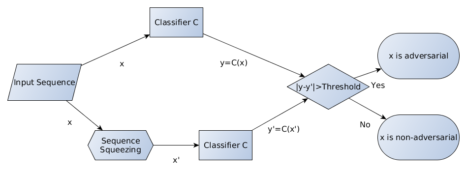
Figure 1: Overview of the Sequence Squeezing Method

Our method is illustrated in Figure 1 and consists of the following stages:

1. Calculate word embedding, representing each API call/word in the vocabulary in a semantic-preserving fashion, that is, words with similar meaning have closer word embeddings.

2. Merge the words closest (=most similar) to a single center of mass in order to reduce the dimensionality of the vocabulary, as well as the adversarial space.

3. Replace all of the words that are part of the merged group with the word closest to the center of mass of this group, maintaining lower dimensionality and keeping the word embeddings used by the original classifier. Thus, we can classify the squeezed input using the original classifier without retraining it.

4. Apply the transformation (steps 1..3) on the classifier’s input sequence. If the classifier’s confidence score for the squeezed sequence is substantially different from the confidence score of the original input (the threshold appears in Equation 3), the sample is adversarial.

The input sequence transformation is shown in Algorithm 1.

1 Input: $D$ (vocabulary), $X_{train}$ (training set of sequences of tokens from $D$), $sizeD_{squeezed}$ (size of squeezed vocabulary)

2 $embed=GloVe(D,X_{train})$ # $embed\in\mathbb{R}^{|D|\times d}$

3$newEmbed=embed$

4for each word embedding $\boldsymbol{\boldsymbol{w_{i}}}$ in $embed$:

5    $embedMergeHashTable[\boldsymbol{w_{i}}]=\left\{\boldsymbol{w_{i}}\right\}$

6while $(width(newEmbed)>sizeD_{squeezed})$:

7    for the two Euclidean closest word embeddings in $newEmbed$, $\boldsymbol{w_{i}},\boldsymbol{w_{j}}$:

8        $\boldsymbol{w_{merged}}=\frac{\boldsymbol{w_{i}}*|embedMergeHashTable[\boldsymbol{w_{i}}]|+\boldsymbol{w_{j}}*|embedMergeHashTable[w_{j}]|}{|embedMergeHashTable[\boldsymbol{w_{i}}]|+|embedMergeHashTable[w_{j}]|}$

9        # Calculate center of mass for the merged embedding

10        $mergedGroup=embedMergeHashTable[\boldsymbol{w_{i}}]\cup embedMergeHashTable[w_{j}]$

11        # The merged count is the aggregated count

12        remove $\boldsymbol{w_{i}},\boldsymbol{w_{j}}$ from $newEmbed$

13        delete $embedMergeHashTable[\boldsymbol{w_{i}}]$

14        delete $embedMergeHashTable[w_{j}]$

15        # Insert the merged embedding $\boldsymbol{w_{merged}}$ instead of $\boldsymbol{w_{i}},\boldsymbol{w_{j}}$

16        insert $\boldsymbol{w_{merged}}$ to $newEmbed$

17        $embedMergeHashTable[\boldsymbol{w_{merged}}]=mergedGroup$

18        # $width(newEmbed)$ was decremented by 1

19for each word embedding $\boldsymbol{w_{new}}$ in $newEmbed$:

20    if $|embedMergeHashTable[\boldsymbol{\boldsymbol{w_{new}}}]|>1$

21    # Meaning: $\boldsymbol{\boldsymbol{w_{new}}}$ is a merged word embedding

22        replace $\boldsymbol{w_{new}}$ with the Euclidean closest word embedding in $embedMergeHashTable[\boldsymbol{\boldsymbol{w_{new}}}]$

return $newEmbed$

Algorithm 1 Sequence Squeezing for API Calls and Words

We used GloVe [39] word embedding, which, in contrast to other methods (e.g., word2vec), has been shown to work effectively with API call traces [24], in order to generate $embed$, the word embedding matrix (of size:$|D|\times d$, where $d$ is the embedding dimensionality) for each API call/word (line 2). This word embedding is robust enough for domains with larger vocabularies, to make our attack applicable to other domains such as NLP .

We then perform agglomerative (bottom-up) hierarchical clustering on the word embeddings, merging the closest word embedding (using Euclidean distance, as in [6] - line 7, as no significant improvement was observed when using cosine distance. For word embedding, by definition, small Euclidean indeed distance implies close semantic meaning). Each time we merge two embeddings, we replace them with their center of mass, which becomes the embedding of the merged group to which each of the merged embedding is mapped (lines 10-17). This use of the center of mass preserves the overall semantic of the group and allows us to keep merging the most semantically similar words into groups (even to groups which were previously merged).

After the merging has been completed, we replace each merged group’s center of mass embedding with the closest (based on the Euclidean distance) original word merged into it, so we can use the original classifier trained on the original embeddings (line 16). The rationale for this is that we want to choose the API or word with the closest semantic meaning to the merged group members (represented by the merged group’s center of mass embedding), in order to maintain the performance of the original classifier.

To detect adversarial examples, we run the original classifier twice: once for the original input and a second time for the sequence squeezed input. If the difference of the confidence scores of the results is larger than $Threshold_{adv}$, we say that the original input is adversarial. We chose $Threshold_{adv}$ to be the maximum difference between the original input and the squeezed input of all of the samples in the training set. Thus, this is the minimal threshold that would not affect the training set classification (and thus the original classifier training). Additional details are available in Section IV-C1.

$$Threshold_{adv}=\max(|f(\boldsymbol{x})-f(\boldsymbol{x_{squeezed}})|)$$ (3)

$$s.t.\>\boldsymbol{x}\in X_{train},$$

$$\boldsymbol{x_{squeezed}}=Algorithm1(D,X_{train},sizeD_{squeezed})[\boldsymbol{x}]$$

The defense method training overhead is low and only involves iterating the training set to calculate the squeezing transformation. No classifier retraining with the squeezed vectors takes place. The original classifier is still being used.

The inference overhead is also low: classifying each sample twice (once with the original input sequence and a second time with the squeezed sequence) using the original classifier.

III-B2 Defense Sequence-GAN

One way to filter out the perturbations added by adversarial attack is to train a GAN to model the distribution of unperturbed input. At inference time, the GAN output (which does not contain the out-of-distribution perturbation) that is closest to the target classifier’s input is found. This input is then fed to the classifier instead, and its prediction is used as the prediction of the original input.

Samangouei et al. [42] presented Defense-GAN, in which a GAN was trained to model the distribution of unperturbed images. However, Defense-GAN is defined for real-valued data only, while API calls of a malware classifier are discrete symbols. Small perturbations required by such GANs are not applicable to discrete API calls.

For instance, you can’t change WriteFile() to WriteFile()+0.001 in order to estimate the gradient needed to perturb the adversarial example in the right direction; you need to modify it such that it is an entirely different API.

The discrete outputs from the generative model make it difficult to pass the gradient update from the discriminative model to the generative model. We therefore used sequence GANs, i.e., GAN architectures designed to produce sequences, in order to adapt this method for input sequences.

Several sequence GAN types were evaluated. For each sequence GAN type, we trained a sequence GAN per class. In this study, this means that a “benign sequence GAN” is used to produce API call sequences drawn from the benign distribution used to train the GAN (the GAN is trained using benign samples from the dataset; see Section IV-C2). A “malicious sequence GAN” is used to produce malicious API call sequences (the GAN is trained using malicious samples from the dataset; see Section IV-C2).

For any input sequence to be classified, $m$ benign API call sequences are generated by the “benign GAN,” and $m$ malicious API call sequences are generated by the “malicious GAN.” We calculate the Euclidean distance (no significant improvement was observed when using the cosine distance) between the input and each of the $2m$ generated sequences, choosing the sequence nearest to the original input sequence. We then return the classifier’s prediction for the nearest sequence to the input sequence. The defense sequence GAN method is illustrated in Figure 2.

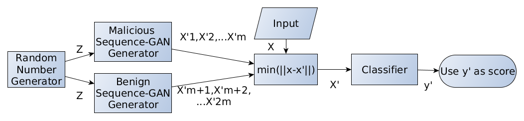
Figure 2: Overview of the defense sequence GAN Method

We have evaluated the following sequence GAN types:

SeqGAN

In SeqGAN [50] implementation, a discriminative model is trained to minimize the binary classification loss between real benign API call sequences and generated ones. In addition to the pretraining procedure that uses the MLE (maximum likelihood estimation) metric, the generator is modeled as a stochastic policy in reinforcement learning (RL), bypassing the generator differentiation problem by directly performing a gradient policy update. Given the API sequence $s_{t}=\left[x_{0},x_{1},..x_{t-1}\right]$ and the next API to be sampled from the model $x_{t}\sim\left(x|s_{t}\right)$, the RL algorithm, REINFORCE, optimizes the GAN objective:

$$\underset{\phi}{\min}-\underset{Y\sim p_{data}}{E}\left[logD_{\phi}(Y)\right]-\underset{Y\sim G_{\Theta}}{E}\left[log(1-D_{\phi}(Y))\right]$$ (4)

The RL reward signal comes from the GAN discriminator, judged on a complete sequence, and is passed back to the intermediate state-action steps using Monte Carlo search, in order to compute the Q-value for generating each token. This approach is usedfor variance reduction.

TextGAN

Zhang et al. [51] proposed a method that optimizes the maximum mean discrepancy (MMD) loss, which is the reconstructed feature distance, by adding a reconstruction term in the objective.

GSGAN

The Gumbel-Softmax trick is a reparametrization trick used to replace the multinomial stochastic sampling in text generation [30]. GSGAN uses $argmax[softmax(h+g)]\backsim softmax(h)$, where $g$ is a Gumbel distribution with zero mean and unit variance. Since this process is differentiable, backpropagation can be directly applied to optimize the GAN objective.

MaliGAN

The basic structure of MaliGAN [13] follows that of SeqGAN. To stabilize the training and alleviate the gradient saturating problem, MaliGAN rescales the reward in a batch.

In this case, the defense method training overhead is high: training two GANs with stable performance is challenging, as discussed in [7].

The inference overhead is also high: generating $2m$ sequences using the two GANs and finding the minimal distance from the input sequence. This defense method’s overhead may not be practical for cyber security applications, where adversaries need to be identified in real time.

III-B3 Nearest Neighbor

In this method, instead of returning the classifier score for the input sequence, we return the score of the training set’s sample nearest to it, using the Euclidean distance (again, no significant improvement was observed using the cosine distance).

This method leverages the fact that adversarial examples try to add minimal perturbation to the input sample (Equation 1), so most parts of the input sequence remain identical to the source (in this case, malicious) class, and the distance from it would be minimal, thus classifying the input sequence correctly despite the adversarial perturbation (a discussion on the importance of minimal perturbation in the cyber domain appears in Section IV-B).

Note that this method is similar to the defense sequence-GAN method (presented in Section III-B2), however, instead of using the GAN output closest to the input sequence, we use the training set sample closest to the input sequence.

This defense method has no training overhead (the classifier training does not change).

However, the inference overhead is high: finding the minimal distance of the input sequence from all of the training set vectors. This is especially true for large training sets, as used by most real world commercial models.

This overhead can be reduced, e.g., by clustering all of the training set vectors, and then calculating the distance to each sample in the closest clusters. However, the overhead problem still exist for large training sets. Another approach is using the input sequence distance only from the centroids. However, this would negatively affect the method’s detection rate due to the lower granularity.

III-B4 RNN Ensemble

An ensemble of models represents a detour from the basic premise of deep neural networks (including recurrent neural networks): training a single classifier on all of the data to obtain the best performance, while overfitting is handled using different mechanisms, such as dropout.

However, an ensemble of models can be used to mitigate adversarial examples. An adversarial example is crafted to bypass a classifier looking at all of the input. Thus, an ensemble of models, each focusing on a subset of the input features, is more robust, since the models trained on the input subsets would not be affected by perturbations performed on other input subsets. Since adversarial examples are usually constructed with a minimum amount of localized perturbations in the input sequence (Equation 1; see discussion in Section IV-B), they would affect only a small number of models, but would be detected by, e.g., ensemble majority voting.

The use of an ensemble of models as a defense method against adversarial examples for images was suggested in [44]. However, the authors only presented the first two types of models mentioned in our paper (regular and bagging) and only a single decision method (hard voting), while we leverage ensemble models that provide better accuracy for sequence based models, e.g., subsequence models.

We evaluate four types of ensemble models:

1. Regular models - Each model is trained on the entire training set and all of the input sequences. The difference between the models in the ensemble is due to the training method: each model would have different initial (random) weights and the training optimizer that can converge to a different function in each model, due to the optimizer’s “stochasticness” (e.g., a stochastic gradient descent optimizer picking different sample mini-batches and therefore converges to a different loss function’s local minimum of the neural network). This means that each neural network learns a slightly different model.

2. Bagging models - Bagging [11] is used on the training set. In those models, the training set consists of drawing $|X_{train}|$ samples with replacement from the training dataset of $|X_{train}|$ samples. On average, each model is trained on 63.02% of the training set, where many samples appear more than once (are oversampled) in the new training set.
   This means that each model is trained on a random subset of the training set samples. Thus, each model learns a slightly different data distribution, (hopefully) making it more robust to adversarial examples generated to fit the data distribution of the entire dataset.
   While our models were trained using dropout (see Appendix B), bagging and dropout are not equivalent: Dropout does not filter entire samples of the training set (only specific neurons from the neural network) or oversample them, as bagging does. Dropout is also applied randomly per epoch and per sample, while a bagging model’s training set is deterministic.

3. Adversarial models - We start from regular models ensemble mentioned above. For each model in the ensemble, adversarial examples are generated and the model is replaced with a model trained on the original model training set and the generated adversarial examples. Thus, these are actually regular models trained using adversarial training (see Section III-B6).

4. Subsequence models - Since the classifier’s input is sequential, we can train each model on a subset of the input sequence, starting from a different offset. That is, if our model is being trained over sequences of 200 API calls, we can split the model into 10 submodels: one on API calls 1..100, the second on API calls 11..110, and the tenth on API calls 101..200.
   Note that the starting offsets can also be randomized per submodel, instead of fixed as was done in our research.
   The idea is that the models which classify an API trace of an adversarial example in a subsequence without a perturbed part (i.e., a purely malicious trace) would be classified correctly, while the perturbed parts would be divided and analyzed separately, making it easier to detect that the trace is not benign.

Additional details are available in Section IV-C4.

The output of the ensemble was calculated using one of two possible methods:

1. Hard voting - Every model predicts its own classification, and the final classification is selected by majority voting between the models in the ensemble.

2. Soft voting - Every model calculates its own confidence score. The average confidence score of all of the models in the ensemble is used to determine the classification. Soft voting gives “confident” models in the ensemble more power than hard voting.

This defense method does not require knowledge about the adversarial examples during its setup in order to mitigate them, making it attack-agnostic, with the exception of adversarial models, which are attack-specific, based on the definition provided earlier in Section III.

This defense method training overhead is high: training the number of models in the ensemble instead of a single model.

The inference overhead is also high: running an inference for each model in the ensemble instead of once.

III-B5 Adversarial Signatures (a.k.a. Statistical Sequence Irregularity Detection)

Adversarial examples are frequently out-of-distribution samples. Since the target classifier was not trained on samples from this distribution, generalization to adversarial examples is difficult. However, this different distribution can also be used to differentiate between adversarial and non-adversarial samples. Our method searches for subsequences of API calls that exist only (or mainly) in adversarial examples, and not in regular samples, in order to detect if the sample is adversarial. We call those subsequences adversarial signatures.

Grosse et al. [20] leverage the fact that adversarial samples have a different distribution than normal samples for non-sequential input. The statistical differences between them can be detected using a high-dimensional statistical test of maximum mean discrepancy. In contrast, our method handles sequential input and leverages the conditional probabilities between the sequence elements (API calls or words) instead of the maximum mean discrepancy.

In order to do that, we start from the observation that in an API call trace, as well as in natural language sentences, there is a strong dependence between the sequence elements. The reason for this is that an API call (or a word in NLP) is rarely independent, and in order to produce usable business logic, a sequence of API calls (each relying on the previous API calls’ output and functionality) must be implemented. For instance, the API call closesocket() would appear only after the API call socket(). The same is true for sentences: an adverb would follow a verb, etc.

For most state-of-the-art adversarial examples, only a small fraction of API calls is added to the original malicious trace (see discussion about minimal perturbation in the cyber security domain in Section IV-B), and the malicious context (the original surrounding API calls of the original business logic) remains. Thus, we evaluated the probability of a certain API call subsequences to appear, generating “signatures” of API call subsequences that are more likely to appear in adversarial sequences, since they contain API calls (the adversarial-added API calls) unrelated to their context.

We decided to analyze the statistical irregularities in n-grams of consecutive API calls. The trade-off when choosing n is to have a long enough n-gram to capture the irregularity in the proper context (surrounding API calls), while remaining short enough to allow generalization to other adversarial examples.

For each unique API call (the features used in [41, 25]) n-gram, we calculate the adversarial n-gram probability of the n-gram of monitored API calls $(w_{1},w_{2}..,w_{n})|\{w_{1},w_{2}..,w_{n}\}\subseteq D$, where $D$ is the vocabulary of available features. Here those features are all of the API calls recorded by the classifier.

$$p_{adv}(w_{1},w_{2}..,w_{n})=$$ (5)

$$\frac{|\left\{x|x\in X_{adv}\wedge((w_{1}\perp w_{2}\perp..w_{n})\subseteq x)\right\}|}{|\left\{x|x\in\left(X_{adv}\cup X_{train,target}\right)\wedge((w_{1}\perp w_{2}\perp..w_{n})\subseteq x)\right\}|}$$

$\perp$ is the concatenation operation. The adversarial n-gram probability is the ratio of occurrences of the n-gram in the adversarial example dataset available to the defender $X_{adv}$, as part of the occurrences in both the adversarial examples and target (i.e., benign) class samples in the training set, $X_{train,target}$.

Note that the equation is valid regardless of $|X_{adv}|$, and there is no assumption regarding the ratio between $|X_{adv}|$ and $|X_{train,target}|$.

The reason we don’t include malicious samples is that we want statistical irregularities from the target class, which is the benign class in this case. Also note that we only look at the appearance of the signatures in the target class and not in other classes (i.e., we look only at the benign class and not the malicious class). The reason for this is that it makes sense that $X_{adv}$ would contain API n-grams available in the source class (the malicious class in this case), because in practice, it is a source class sample.

We say that the n-gram of monitored API calls $(w_{1},w_{2}..,w_{n})$ is an adversarial signature if the adversarial n-gram probability of this n-gram is larger than a threshold $ThresholdP_{adv}$ that is determined by the trade-off between the adversarial example detection rate and the number of target class samples falsely detected as adversarial; the higher the threshold, the lower both would be.

We classify a sample as an adversarial example if it contains more than $ThresholdSigs_{adv}$ adversarial signatures. The more irregular n-grams detected, the more likely the sequence is to be adversarial. Additional details are provided in Section IV-C5.

This defense method requires a dataset of adversarial examples, $X_{adv}$, during its setup, in order to make it robust against such examples, making it attack-specific, based on the definition provided earlier in Section III.

Note that while finding “non-adversarial signatures” using this method is possible, it is more problematic, especially when $|X_{train,target}|$ is very large. Other methods presented in this paper, such as defense sequence GAN (see Section III-B2), implement this approach more efficiently.

This defense method training overhead is high: counting all subsequences of a certain size in the training set.

The inference overhead, however, is low: searching for the adversarial signatures in the input sequence.

III-B6 Adversarial Training

Adversarial training is the method of adding adversarial examples, with their non perturbed label (source class label), to the training set of the classifier. The rationale for this is that since adversarial examples are usually out-of-distribution samples, inserting them into the training set would cause the classifier to learn the entire training set distribution, including the adversarial examples.

Additional details are available in Section IV-C6.

Unlike all other methods mentioned in this paper, this method has already been tried for sequence based input in the NLP domain ([6, 33]), with mixed results about the robustness it provides against adversarial attacks. Additional issues regarding this method are described in Section II-B. We evaluate this method in order to determine whether the cyber security domain, with a much smaller dictionary (less than 400 API call types monitored in [41] compared to the millions of possible words in NLP domains), would yield different results. We also want to compare it to the defense methods presented in this paper, using the same training set, classifier, etc.

This defense method training overhead is high (generating many adversarial examples, following by training a classifier on a training set containing them).

There is no inference overhead: the inference is simply performed using the newly trained classifier.

IV Experimental Evaluation

IV-A Dataset and Target Malware Classifiers

We use the same dataset used in [41], because of its size: it contains 500,000 files (250,000 benign samples and 250,000 malware samples), faithfully representing the malware families in the wild and allowing us a proper setting for attack and defense method comparison. Details are provided in Appendix A.

Each sample was run in Cuckoo Sandbox, a malware analysis system, for two minutes per sample. Tracing only the first few seconds of a program execution might not allow the detection of certain malware types, like “logic bombs” that commence their malicious behavior only after the program has been running for some time. However, this can be mitigated both by classifying the suspension mechanism as malicious, if accurate, or by tracing the code operation throughout the program execution lifetime, not just when the program starts. The API call sequences generated by the inspected code during its execution were extracted from the JSON file generated by Cuckoo Sandbox. The extracted API call sequences were used as the malware classifier’s features.

The samples were run on Windows 8.1 OS, since most malware targets the Windows OS. Anti-sandbox malware was filtered to prevent dataset contamination (see Appendix A). After filtering, the final training set size is 360,000 samples, 36,000 of which serve as the validation set. The test set size is 36,000 samples. All sets were balanced between malicious and benign samples, with the same malware families composition as in the training set.

There are no commercial trial version or open-source API call based deep learning intrusion detection systems available (such commercial products target enterprises and involve supervised server installation). Dynamic models are also not available in free online malware scanning services like VirusTotal. Therefore, we used RNN based malware classifiers, trained on the API call traces generated by the abovementioned dataset.

The API call sequences were split into windows of $m$ API calls each, and each window was classified in turn. Thus, the input of all of the classifiers was a vector of $m=140$ (larger window sizes didn’t improve the classifier’s accuracy) API call types, each with 314 possible values (those monitored by Cuckoo Sandbox). The classifiers used to evaluate the attacks are similar to those used in [41]. Their implementation and hyperparameters (loss function, dropout, activation functions, etc.), and the performance of the target classifiers are described in Appendix B.

IV-B Evaluated Attacks

The attacks used to assess the defense methods’ robustness are described in Appendix C. These are the state-of-the-art out of the few published RNN attacks in the cyber security domain. The attacks add API calls to the API trace (not removing or modifying API calls, in order to avoid damaging the modified code’s functionality) based on either their gradients, maximizing the effect of each added API call, or randomly. The maximum number of allowed adversarial API calls is 93 in each sliding window of $n=140$ API calls (i.e., 66.67% which is a very permissive boundary).

Three attacks are used to evaluate the robustness of our defense methods:

1. A realistic gradient based black-box attack, in which the attacker has no knowledge of the target classifier’s architecture or weights and has to build a substitute model, as done in [41]. The holdout dataset size to build the substitute model was identical (70 samples) for a fair comparison. The attack effectiveness for the LSTM classifier (without any defense method) is 99.99%.

2. A white-box gradient based attack, where the adversary uses the target classifier instead of a substitute model. This attack is a stronger variant of the attack used in [40], which has access only to the confidence score of the classifier. The attack effectiveness for the LSTM classifier (without any defense method) is 100.00%

3. An adaptive attacker white-box attack, where the attacker is aware not only of the classifier’s architecture and hyperparameters, but also of the defense method being used. Thus, the attacker operates an adversarial attack specially crafted for the used defense method. These attacks are described per defense method in Section IV-C. All of these attacks’ effectiveness for the LSTM classifier is 100%.

4. A random perturbation attack. The attack effectiveness for the LSTM classifier (without any defense method) is 22.97% (average of five runs).

Adversarial attacks against images usually try to minimize the number of modified pixels in order to evade human detection of the perturbation. One might claim that such a definition of minimal perturbation is irrelevant for API call traces: humans cannot inspect sequences of thousands or millions of APIs, so an attacker can add an unlimited amount of API calls, this improving the attack effectiveness against the evaluated defense methods.

However, one should bear in mind that malware aims to perform its malicious functionality as quickly as possible. For instance, ransomware usually starts by encrypting the most critical files (e.g., the ’My Documents’ folder) first, so even if the user turns off the computer and sends the hard drive to the IT department - damage has already been done. The same is true for a keylogger that aims to send the user passwords to the attacker as soon as possible, so they can be used immediately, before the malware has been detected and neutralized.

Moreover, adding too many API calls would cause the program’s profile to become anomalous, making it easier to detect by anomaly detection intrusion detection systems, e.g., those that measure CPU usage [36], or contain irregular API call subsequences (Section III-B5).

Finally, the robustness of the defense methods to the addition of many API calls is being evaluated by the random perturbation attack. The random attack adds 50% API calls to the trace, as opposed to 0.0005% API calls for the entire trace for the gradient based black-box and white-box attacks [41]. or 10,000 times more API calls, buy has much lower evasion rate. Thus, samples whose adversarial variants are detected cannot evade detection simply by adding more perturbations.

IV-C Defense Methods Implementation Details

Additional details about the implementation of the defense methods are provided in the subsections that follow. Each subsection also contains a description of the best adaptive white-box attack against this method, that is, if the attacker knows this method is being used, how can he/she bypass it most effectively.

IV-C1 Sequence Squeezing

We used Stanford’s GloVe implementation [3] with embedding dimensionality of $d=32$. The vocabulary $D$ used by our malware classifiers contains all of the API calls monitored by Cuckoo Sandbox, documented in the Cuckoo Sandbox repository [1].

Running Algorithm 1 on our training set (see Section IV-A) of API call traces resulted in interesting sequence squeezing. It seems that the squeezed groups maintained the “API contextual semantics” as expected, merging, for instance, the variants of the same API, e.g., GetUserNameA() and GetUserNameW(). Other merged API calls are different API calls with the same functionality, e.g., socket() and WSASocketA().

The sequence squeezing we used, with $sizeD_{squeezed}=\left\lceil\frac{|D|}{2}\right\rceil=157$, is described in Appendix D. Using smaller feature spaces, e.g., $sizeD_{squeezed}=\left\lceil\frac{|D|}{3}\right\rceil$, resulted in the inability to maintain the “API contextual semantics,” merging unrelated API calls and reducing the classifier’s accuracy by 7%. However, using larder feature spaces, e.g., $sizeD_{squeezed}=\left\lceil\frac{2|D|}{3}\right\rceil$,did not limit the adversarial space enough, resulting in 5% adversarial recall loss. For our training set, we used $Threshold_{adv}=0.18$.

Other hyperparameters (grid-search selected) were less effective.

Best Adaptive White-Box Attack

To bypass sequence squeezing defense method, the attacker performs the white-box attack (described in Section IV-B) twice: once on the original input sequence (generating the adversarial example $\boldsymbol{x}^{*}$) and once on the squeezed sequence (generating the adversarial example $\boldsymbol{x_{squeezed}^{*}}$), both of them using perturbation only from the squeezed vocabulary $D_{squeezed}$, and not from $D$. This is done iteratively, until we bypass the threshold being set in Equation 3: $Threshold_{adv}\geq(|f(\boldsymbol{x}^{*})-f(\boldsymbol{x_{squeezed}^{*}})|)$. If this attack doesn’t succeed after 10 iterations, the attack has failed.

IV-C2 Defense Sequence-GAN

To implement the benign perturbation GAN, we tested several GAN types, using Texygen [53] with its default parameters. We used MLE training as the pretraining process for all of the GAN types except GSGAN, which requires no pretraining. In pretraining, we first trained 80 epochs for a generator and then trained 80 epochs for a discriminator. The adversarial training came next. In each adversarial epoch, we updated the generator once and then updated the discriminator for 15 mini-batch gradients. We generated a window of 140 API calls, each with 314 possible API call types, in each iteration.

As mentioned in Section III-B2, we tested several GAN implementations with discrete sequence output: SeqGAN [50], TextGAN [51], GSGAN [30], and MaliGAN [13]. We trained our “benign GAN” using a benign holdout set (3,000 sequences). Next, we generated $m=200$ sequences with the “benign GAN,” using an additional benign hold-out set (3,000 sequences) as a test set. We used the same procedure to train our “malicious GAN” and generated an additional $m=200$ sequences using it.

SeqGAN outperforms all other models by providing the average minimal distance (both the Euclidean distance and cosine distance provided similar results) between the 400 sequences generated and the test set vectors, meaning that the sequences generated were the closest to the requested distribution, thus, we used SeqGAN.

Best Adaptive White-Box Attack

To bypass defense sequence GAN, the attacker performs the white-box attack (described in Section IV-B) and then performs the same process done by the defender in Section III-B2: He/she generates $m=200$ sequences with the “benign GAN,” and generates an additional $m=200$ sequences using the “malicious GAN”. The attacker iteratively repeats this process until the adversarial sequence is closer to one of the benign GAN sequences which are classified as benign. If this attack doesn’t succeed after 10 iterations, the attack has failed.

IV-C3 Nearest Neighbor

The cosine distance is more effective than the Euclidean distance in many NLP tasks. However, the differences in performance due to the use of cosine distance instead of Euclidean distance were marginal, as mentioned in Section III-B3. Therefore, we used the Euclidean distance for nearest neighbor calculations.

Best Adaptive White-Box Attack

To bypass the nearest neighbor defense method, the attacker iteratively performs the white-box attack (described in Section IV-B) and then calculates the distance to the nearest neighbor in the training set, until this neighbor’s classification is benign. If this attack doesn’t succeed after 10 iterations, the attack has failed.

IV-C4 RNN Ensemble

We used six variants of ensembles, each consisting of nine models:

• Regular ensemble - Each model was trained on the entire dataset.

• Subsequence ensemble - The first model is trained on API calls at offsets between 1..140 in the API call trace, the second model is trained on API calls at offsets 11…150 in the API call trace, etc. The ninth model is trained on API calls at offsets 91..230 in the API call trace.

• Bagging ensemble - Each model is trained on a random subset of the dataset, as discussed in Section III-B4.

• Bagging subsequence ensemble - This is a combination of the bagging and subsequence ensembles. Each model is trained not only on a different API call offset range (like the regular subsequence ensemble described above) but also on a random subset of the training set, as in the bagging ensemble.

• Adversarial ensemble - Each model has 14,000 (out of 27,000) malicious samples replaced with their adversarial example variants, similar to adversarial training (see Section IV-C6).

• Adversarial subsequence ensemble - This is a combination of the adversarial and subsequence ensembles. The adversarial examples’ API call traces used for training also start at an offset.

The output of the ensemble presented in Table II was made using soft voting (see Section III-B4). However, the difference between soft and hard voting in all of our tests was marginal.

Best Adaptive White-Box Attack

To bypass RNN ensemble defense method, the attacker performs the white-box attack (described in Section IV-B) on each classifier in the ensemble in turn, and aggregates the added adversarial API calls from all the attacks into the same adversarial sequence.

IV-C5 Adversarial Signatures

We chose $n=5$, i.e., we used 5-grams of API calls for the “adversarial signatures.” Shorter API call subsequences caused more “adversarial false positives,” i.e., identifying regular samples as adversarial (e.g., $n=4$ resulted in 0.5% of the test set incorrectly classified as adversarial), while longer API call sequences were too specific to detect the majority of the adversarial examples (e.g., $n=6$, while having optimal performance in other systems [46], resulted in a 15% loss of adversarial recall).

We used $ThresholdP_{adv}=1.0$, thus, we looked for API subsequences which appear only in adversarial examples. We also used $ThresholdSigs_{adv}=1$, so that in order to classify a sample as an adversarial example, it is enough that it contains a single adversarial signature.

Other hyperparameters (grid search selected) were less effective.

Best Adaptive White-Box Attack

To bypass adversarial signatures, the attacker performs the white-box attack (described in Section IV-B), but verifies for each added adversarial API call that its addition generates no adversarial signatures. If it does, the attacker would choose a different position in the sequence instead to add a different adversarial API call, by re-calculating the gradients, as described in Appendix C.

IV-C6 Adversarial Training

We ran the adversarial black-box and white-box attacks (see Appendix C), as suggested in [34], on the training set. We generated 14,000 malicious adversarial examples (50% generated by the black-box attack and 50% by the white-box attack), which replaced 14,000 malicious samples in the original training set. Other sizes (grid search selected) resulted in reduced accuracy.

Best Adaptive White-Box Attack

To bypass adversarial training, the attacker performs the white-box attack (described in Section IV-B) on the classifier trained on the augmented training set that includes the adversarial examples, either.

IV-D Defense Method Performance

The different defense methods mentioned in Section III are measured using two factors:

The adversarial recall is the fraction of adversarial sequences generated by the attack which were either detected by the defense method or classified as malicious by the classifier. Adversarial recall provides a metric for the robustness of the classifier combined with a defense method against a specific adversarial attack.

The classifiers’ accuracy, which applies equal weight to both false positives and false negatives (unlike precision or recall), thereby providing an unbiased overall performance indicator. The accuracy is evaluated against the regular test set only (that is, without adversarial examples). Using this method, we verify the effect our defense methods have on the classifiers’ performance for non-adversarial samples. Since samples classified as adversarial examples are automatically classified as malicious (because there is no reason for a benign adversarial example), every benign sample classified as an adversarial example would damage the classifier’s accuracy. Therefore, we also specify the false positive rate of the classifier to better asses the effect of those cases.

The performance of the attack versus the various defense methods and the classifier’s performance using those defense methods for the LSTM classifier (see Appendix B; note that the other tested classifiers mentioned in Appendix B behave the same) are presented in Table II. All adaptive white-box attacks were tried against all defense methods, but only the best one (with the lowest adversarial recall) is shown in the table, due-to space limits.

The overhead column contains high-level observations regarding the defense method’s overhead (none, low, or high), both during training (time and money) and during inference (run-time performance). The analysis is described in detail in the subsections of Section III. As models get more complicated and larger in size, we would expect defense methods with lower overhead to be more easily deployed in real-world scenarios.

TABLE II: Defense Method Performance

Defense Method	Adversarial Recall [%], Best Adaptive White-Box Attack	Adversarial Recall [%], White-Box Attack	Adversarial Recall [%], Black-Box Attack	Adversarial Recall [%], Random Perturbation Attack (Average of 5 Runs)	Classifier Accuracy/False Positive Rate [%], Non-Perturbed Test Set	Method Overhead (Training/ Inference)
Original Classifier (No Defense Methods)	-	-	-	-	91.81/0.89	None/None
Sequence Squeezing	38.76	86.96	48.57	99.14	90.81/0.99	Low/Low
Defense Sequence-GAN	13.18	50.49	57.38	97.35	64.55/3.85	High/High
Nearest Neighbor	11.68	88.78	56.12	40.56	87.85/1.32	None/High
RNN Ensemble (Regular)	19.65	47.91	73.0	84.54	92.59/0.81	High/High
RNN Ensemble (Subsequence)	22.72	86.27	56.79	85.55	92.27/0.84	High/High
RNN Ensemble (Bagging)	18.23	47.90	73.01	87.29	92.65/0.80	High/High
RNN Ensemble (Bagging Subsequence)	24.15	86.26	56.78	79.00	90.54/1.03	High/High
RNN Ensemble (Adversarial)	21.17	47.92	73.02	99.57	92.97/0.76	High/High
RNN Ensemble (Adversarial Subsequence)	27.19	86.27	56.79	99.34	92.21/0.85	High/High
Adversarial Signatures	11.65	75.36	75.38	99.78	91.81/0.89	High/Low
Adversarial Training	11.16	48.32	12.39	99.09	91.81/0.91	High/None

We see that certain defense methods, such as RNN subsequence ensembles and adversarial signatures, provide good robustness against adversarial attacks (75-85% adversarial recall). Ensemble models also improve the classifier performance on non-adversarial samples. However, our novel defense method, sequence squeezing, provides a much lower overhead than all the other methods, while still offering good robustness against adversarial attacks, making it the most suited for real world scenarios and especially when real time classification is required, like in the cyber security domain. Sequence squeezing is also the best method against an adaptive attacker, leaving the defender better off than with any other evaluated defense method.

IV-E Discussion

Table II reveals several interesting issues:

We see that the best defense method selection depends on the specific scenario:

• When the training and inference overhead is not a concern, an RNN subsequence ensemble provide good robustness against adversarial attacks (especially white-box attacks, both adaptive and not) while improving the classifier performance on non-adversarial samples.

• When an attack-specific defense is acceptable, adversarial signatures provide good robustness against adversarial attacks (especially black-box attacks), with lower overhead.

• Finally, for cases where a low overhead attack-agnostic defense method is required (as required in most real world scenarios), the novel sequence squeezing defense method provides good robustness against adversarial attacks, with much lower overhead, at a price of a slight degradation in the classifier performance against non-adversarial samples (0.1% addition to the false positive rate). This means that sequence squeezing is the best choice for cyber security applications, where on the one hand, adversaries need to be identified in real time, but on the other hand, the adversarial attack method is unknown, so attack-specific method like adversarial signatures is irrelevant.

Attack-specific defense methods (adversarial signatures, adversarial training) present very poor adversarial recall against the best adaptive white-box attack. Attack-agnostic defense methods which rely on the assumption that the attacker would use minimal perturbation (defense sequence GAN, nearest neighbor) provide slightly better performance, but still cannot cope with attackers that use larger perturbations. Our novel defense method, sequence squeezing, is the best one against adaptive attacks. The reason is sequence squeezing reduces the dimensionality of the possible adversarial perturbations, limiting the attacker’s possibilities to perturb the input and evade detection,

The evaluated defense methods usually provide greater robustness against white-box attacks than against black-box attacks. This suggests that transferable adversarial examples, the ones that bypass the substitute model and are also effective against another classifier (the target model), as done in the black-box attack, are different from other adversarial examples (e.g., drawn from a different distribution), causing defense methods to be less effective against them. For instance, transferable adversarial examples might contain adversarial API calls with similar semantic meaning to the API calls of the original benign sample, making sequence squeezing less effective. Analyzing the differences between black-box and white-box RNN adversarial examples and their effect on our proposed defense methods will be addressed in future work.

All of the evaluated defense methods provide adequate robustness against a random perturbation attack. However, as shown earlier in Section IV-D, this attack is less effective than other attack types and is ineffective even when no defense method is applied.

The accuracy of the RNN ensembles is higher than the original classifier for all ensemble types. The RNN subsequence ensembles also provide good robustness against white-box attacks, while the non-subsequence ensembles provide good robustness against black-box attacks. Bagging and adversarial models do not affect the performance when adding them to the subsequence or regular models.
On the other hand, an ensemble requires the training of many models. This affects both the training time and the prediction time: An ensemble of nine models like in this study, requires nine times the training and inference time of a single model.
One might claim that the improvement of RNN subsequence ensemble classifiers on non-adversarial samples results from the fact that those classifiers consider more API calls in each sliding window (230 API calls in all nine models, instead of 140 API calls in a single model). However, testing larger API call sliding windows for a single classifier (1000 API calls in [41]) did not result in a similar improvement. This leads us to believe that the improved performance actually derives from the ensemble itself and not from the input size. This is supported by the improvement in non-subsequence ensembles.

The sequence squeezing defense method provides good robustness against white-box attacks but is less effective against black-box attacks. This defense method causes a small decrease in the classifier performance (about 1%) and doubles the prediction time, because two models are being run: the original and the sequence squeezed models.

The adversarial signatures defense method provides the best black-box attack robustness, but its white-box attack performance is lower than sequence squeezing.

The only published defense method to date, adversarial training, underperforms in comparison to all other defense methods evaluated, since its adversarial recall is lower.

For the defense sequence GAN method, the inability of the sequence based GANs to capture the complex input sequence distribution (demonstrated, for instance, by the fact that some of the API sequences generated by the GAN contain only a single API call type, as opposed to the training set benign samples), causes its classifier accuracy against non-adversarial samples to be the lowest of all other defense methods and the original classifier, making defense sequence GAN unusable in real-world scenarios.

Given the low accuracy of the classifier on non-adversarial samples when using the defense sequence GAN method, as opposed to the good performance of Defense-GAN in the image recognition domain [42], we hypothesize that the problem is due to the fact that the sequence based GANs we used (like SeqGAN) were unable to capture the true distribution of the input sequence and produced bad seqence GAN output. This was validated by analyzing the nearest neighbor defense method’s performance.
We see that for the nearest neighbor defense method, both the classifier accuracy for non-adversarial test set and the adversarial recall are higher. This suggests that a larger sequence GAN training set (which would require a stronger machine with more GPU memory than that used in this research) would result in a better approximation of the input sequence distribution by the sequence GAN and thus allow defense sequence GAN to be as effective as the nearest neighbor defense method - and more generalizable to samples significantly different from the training set. Such experiments are planned for future work.
The nearest neighbor method also has its limitations: its adversarial recall against random perturbations is low, since this attack method adds, on average, more than 50% new, random API calls. In this case, the nearest neighbor is more likely to be a benign sample, causing an adversarial example to be missed.

V Conclusions and Future Work

In this paper, we present a novel defense method against RNN adversarial examples and compare it to a baseline of four defense methods inspired by state-of-the-art CNN defense methods. To the best of our knowledge, this is the first paper to focus on this challenge, which is different from developing defense methods to use against non-sequence based adversarial examples.

We found that sequence squeezing, our novel defense method, is the only method which provides the balance between the low overhead required by real time classifiers (like malware classifiers) and good robustness against adversarial attacks. This makes sequence squeezing the most suited for real world scenarios, and especially for API call based RNN classifiers that need to provide classification in real time, while new classifier input (API calls) is constantly being fed.

Our future work will focus on four directions:

1. Investigating additional defense methods (e.g., using cluster centroid distance instead of nearest neighbors to improve run-time performance) and evaluating the performance obtained when several defense methods are combined.

2. Extending our work to other domains that use input sequences, such as NLP.

3. Observing the performance gap of our defense methods against black-box and white-box attacks (as discussed in Section IV-D) illustrates some interesting questions. For example, we would evaluate the effect of implementing defense methods using white-box adversarial examples, as opposed to black-box examples, which were used in this paper.

The increasing usage of machine learning based classifiers, such as “next generation anti virus,” raises concern from actual adversaries (the malware developers) trying to evade such systems using adversarial learning. Making such malware classifiers robust against adversarial attack is therefore important, and this paper (as well as future research in this domain) provides methods to defend classifiers that use RNNs, such as dynamic analysis API call sequence based malware classifiers, from adversarial attacks.

Appendix A: Tested Dataset

We used identical implementation details (e.g., dataset, classifier hyperparameters, etc.) as [41], so the attacks can be compared. Those details are provided here for the reader’s convenience.

An overview of the malware classification process is shown in Figure 3, as presented in [41].

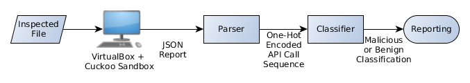
Figure 3: Overview of the Malware Classification Process

The dataset used is large and includes the latest malware variants, such as the Cerber and Locky ransomware families. Each malware type (ransomware, worms, backdoors, droppers, spyware, PUAs, and viruses) has the same number of samples, in order to prevent prediction bias towards the majority class. 20% of the malware families (such as the NotPetya ransomware family) were only used in the test set to assess generalization to an unseen malware family. 80% of the malware families (such as the Virut virus family) were distributed between the training and test sets to determine the classifier’s ability to generalize to samples from the same family. The temporal difference between the training set and the test set is six months (i.e., all training set samples are older than the test set samples), based on VirusTotal’s ’first seen’ date.

The ground truth labels of the dataset were determined by VirusTotal, an online malware scanning service which contains more than 60 different security products. A sample with 15 or more positive classifications (i.e., is considered malicious) from the 60 products is considered malicious by our classifiers. A sample with zero positive classifications is labeled as benign. All samples with 1-14 positives were omitted to prevent false positive contamination of the dataset. Family labels for dataset balancing were taken from the Kaspersky Anti-Virus classifications.

It is crucial to prevent dataset contamination by malware that detects whether the malware is running in a Cuckoo Sandbox (or on virtual machines) and if so, quits immediately to prevent reverse engineering efforts. In those cases, the sample’s label is malicious, but its behavior recorded in Cuckoo Sandbox (its API call sequence) isn’t, due to its anti-forensic capabilities. To mitigate such contamination of the dataset, two countermeasures were used:

1. Considering only API call sequences with more than 15 API calls (as in [26]) and omitting malware that detects a virtual machine (VM) and quits.

2. Applying YARA rules to find samples trying to detect sandbox programs, such as Cuckoo Sandbox, and omitting all such samples.

One might argue that the evasive malware that applies such anti-VM techniques are extremely challenging and relevant, however in this paper, we focus on the adversarial attack. This attack is generic enough to work for those evasive malware as well, assuming that other mitigation techniques (e.g., anti-anti-VM), would be applied.

After this filtering and balancing of the benign samples, about 400,000 valid samples remained. The final training set size is 360,000 samples, 36,000 of which serve as the validation set. The test set size is 36,000 samples. All sets are balanced between malicious and benign samples. Due to hardware limitations, a subset of the dataset was used as a training set: 54,000 training samples and test and validation sets of 6,000 samples each. The dataset was representative and maintained the same distribution as the entire dataset described above.

Appendix B: Malware Classifiers Tested

As mentioned in Section IV, we used the malware classifiers from [41], since many classifiers are covered, allowing us to evaluate the defense performance against many types of classifiers. The maximum input sequence length was limited to $m=140$ API calls, since longer sequence lengths, e.g., $m=1000$, had no effect on the accuracy, and padded shorter sequences with zeros. A zero stands for a null/dummy value API in our one-hot encoding. Longer sequences are split into windows of $m$ API calls each, and each window is classified in turn. If any window is malicious, the entire sequence is considered malicious. Thus, the input of all of the classifiers is a vector of $m=140$ API call types in one-hot encoding, using 314 bits, since there were 314 monitored API call types in the Cuckoo reports for the dataset. The output is a binary classification: malicious or benign.

An overview of the LSTM architecture is shown in Figure 4.

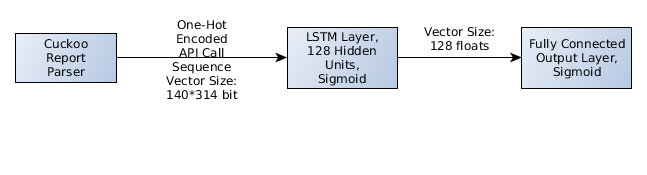
Figure 4: LSTM Classifier Architecture

The Keras implementation was used for all neural network classifiers, with TensorFlow used for the backend.

The loss function used for training was binary cross-entropy. The Adam optimizer was used for all of the neural networks. The output layer was fully connected with sigmoid activation for all neural networks. For neural networks, a rectified linear unit, $ReLU(x)=max(0,x)$, was chosen as an activation function for the input and hidden layers due to its fast convergence compared to $sigmoid()$ or $\tanh()$, and dropout was used to improve the generalization potential of the network. A batch size of 32 samples was used.

The classifiers also have the following classifier-specific hyperparameters:

• RNN, LSTM, GRU, BRNN, BLSTM, bidirectional GRU - a hidden layer of 128 units, with a dropout rate of 0.2 for both inputs and recurrent states.

• Deep LSTM and BLSTM - two hidden layers of 128 units, with a dropout rate of 0.2 for both inputs and recurrent states in both layers.

Classifier performance was measured using the accuracy ratio, which gives equal importance to both false positives and false negatives (unlike precision or recall). The false positive rate of the classifiers varied between 0.5-1%.

The performance of the classifiers is shown in Table III. The accuracy was measured on the test set, which contains 36,000 samples.

TABLE III: Classifier Performance

Classifier Type	Accuracy (%)
RNN	97.90
BRNN	95.58
LSTM	98.26
Deep LSTM	97.90
BLSTM	97.90
Deep BLSTM	98.02
GRU	97.32
Bidirectional GRU	98.04

As can be seen in Table III, the LSTM variants are the best malware classifiers, in terms of accuracy.

Appendix C: Adversarial Attacks Used

We used the adversarial attack implemented in [41], since this is the state-of-the-art adversarial attack in the cyber security domain. An adversarial example is a sequence of API calls classified as malicious by the classifier, which is perturbed by the addition of API calls, so that the modified sequence will be misclassified as benign. In order to prevent damaging the code’s functionality, one cannot remove or modify API calls; one can only add additional API calls. The attack used to evaluate the robustness of our defense method is described in Algorithm 2.

1 Input: $f$ (black-box model), $\hat{f}$ (substitute model), $\boldsymbol{\mathbf{x}}$ (malicious sequence to perturb, of length $l$), $n$ (size of adversarial sliding window), $D$ (vocabulary)

2 for each sliding window $\boldsymbol{\mathbf{w}}_{j}$ of $n$ API calls in $\boldsymbol{\mathbf{x}}$:

3    $\boldsymbol{\boldsymbol{\mathbf{w}}_{j}}^{*}=\boldsymbol{\boldsymbol{\mathbf{w}}_{j}}$

4    while $f(\boldsymbol{\boldsymbol{\mathbf{w}}_{j}^{*}})=malicious$ and the number of modifications in $\boldsymbol{\boldsymbol{\mathbf{w}}_{j}}^{*}<\left\lceil\frac{2n}{3}\right\rceil$:

5        Randomly select an API’s position i in $\boldsymbol{\mathbf{w}}$

6        # Insert a new adversarial API in position $i\in\{1..n\}$:

7     $\boldsymbol{\boldsymbol{\mathbf{w}}_{j}^{*}}[i]=\arg\min_{api}||sign(\boldsymbol{\boldsymbol{\mathbf{w}}_{j}}^{*}-\boldsymbol{\boldsymbol{\mathbf{w}}_{j}^{*}}[1:i-1]\perp api\perp\boldsymbol{\boldsymbol{\mathbf{w}}_{j}^{*}}[i:n-1])-sign(J_{\hat{f}}(\boldsymbol{\boldsymbol{\mathbf{w}}_{j}})[f(\boldsymbol{\boldsymbol{\boldsymbol{w}}_{j}})])||$

8    Replace $\boldsymbol{\mathbf{w}}_{j}$ (in $\boldsymbol{\mathbf{x}}$) with $\boldsymbol{\boldsymbol{\mathbf{w}}_{j}}^{*}$

return (perturbed) $\mathbf{\boldsymbol{x}}$

Algorithm 2 Adversarial Sequence Generation

$D$ is the vocabulary of available features, that is, the API calls recorded by the classifier. The adversarial API call sequence length of $l$ might be different than $n$, which is the length of the sliding window API call sequence that is used by the adversary. Therefore, like the prediction, the attack is performed sequentially on $\left\lceil\frac{l}{n}\right\rceil$ windows of $n$ API calls. We chose $n=m=140$ (the window size of the classifier, mentioned in Appendix B). $\perp$ is the concatenation operation. $\boldsymbol{\boldsymbol{\mathbf{w}}_{j}^{*}}[1:i-1]\perp api\perp\boldsymbol{\boldsymbol{\mathbf{w}}_{j}^{*}}[i:n-1]$ is the insertion of the encoded API vector in position $i$ of $\boldsymbol{\mathbf{w}}_{j}^{*}$. In each window $\boldsymbol{\mathbf{w}}_{j}$, the adversary randomly chooses $i$ since he/she does not have any way to better select $i$ without incurring significant statistical overhead.

Note that an insertion of an API in position $i$ means that the APIs from position $i..n$ ($\boldsymbol{\mathbf{w}}_{j}^{*}[i:n]$ ) are “pushed back” one position to make room for the new API call, in order to maintain the original sequence and preserve the original functionality of the code. Since the sliding window has a fixed length, the last API call, $\boldsymbol{\boldsymbol{\mathbf{w}}_{j}^{*}}[n]$, is “pushed out” and removed from $\boldsymbol{\mathbf{w}}_{j}^{*}$ (this is why the term is $\perp\boldsymbol{\boldsymbol{\mathbf{w}}_{j}^{*}}[i:n-1]$, as opposed to $\perp\boldsymbol{\boldsymbol{\mathbf{w}}_{j}^{*}}[i:n]$). The APIs “pushed out” from $\boldsymbol{\mathbf{w}}_{j}$ will become the beginning of $\boldsymbol{\mathbf{w}}_{j+1}$, so no API is ignored.

The newly added API call is $\boldsymbol{\boldsymbol{\mathbf{w}}_{j}^{*}}[i]=\arg\min_{api}||sign(\boldsymbol{\boldsymbol{\mathbf{w}}_{j}}^{*}-\boldsymbol{\boldsymbol{\mathbf{w}}_{j}^{*}}[0:i]\perp api\perp\boldsymbol{\boldsymbol{\mathbf{w}}_{j}^{*}}[i:n-1])-sign(J_{\hat{f}}(\boldsymbol{\boldsymbol{\mathbf{w}}_{j}})[f(\boldsymbol{\boldsymbol{\boldsymbol{w}}_{j}})])||$. $sign(J_{\hat{f}}(\boldsymbol{\boldsymbol{\mathbf{w}}_{j}})[f(\boldsymbol{\boldsymbol{\boldsymbol{w}}_{j}})])$ gives us the direction in which we have to perturb the API call sequence in order to reduce the probability assigned to the malicious class, $f(\boldsymbol{\mathbf{x}})$, and thus change the predicted label of the API call sequence. However, the set of legitimate API call embeddings is finite. Thus, we cannot set the new API to any real value. We therefore find the API call $api$ in $D$ whose insertion directs us closest to the direction indicated by the Jacobian as most impactful on the model’s prediction. We iteratively apply this heuristic until either the classification of the entire sequence changes (meaning that the classification of each window $\boldsymbol{\mathbf{w}}_{j}$ changes) or until the maximum number of modifications is reached in a certain window: $\left\lceil\frac{2n}{3}\right\rceil$. In the latter case, the attack has failed. The use of a maximum number of allowed perturbations is commonly used in adversarial learning, and a modification of 66.67% of the malware API calls (up to 93 adversarial API calls in each window of $n=140$ API calls) is a very permissive boundary.

Three variants of this attack were used. In the white-box variant, we used $\hat{f}(\boldsymbol{\mathbf{x}})=f(\boldsymbol{\mathbf{x}})$, so the attacker is fully aware of the architecture, weights, and hyperparameters of the target classifier. In the black-box variant, we used a substitute model, as used in [41]. The substitute model was a GRU with 64 units (different from the malware classifiers used in Appendix B). Besides the classifier’s type and architecture, a different optimizer was used for the substitute model (ADADELTA instead of Adam). Finally, in the random perturbation variant, no substitute model was used, and line 7 was replaced with a randomly chosen API call type.

Appendix D: Sequence Squeezing for API Calls Monitored by Cuckoo Sandbox

TABLE IV: Sequence Squeezing for Cuckoo Sandbox Monitored API Calls

CertControlStore	CertControlStore
CertCreateCertificateContext	CertCreateCertificateContext
CertOpenStore	CertOpenStore
CertOpenSystemStoreA	CertOpenStore
CertOpenSystemStoreW	CertOpenStore
CoCreateInstance	CoCreateInstance
CoCreateInstanceEx	CoCreateInstance
CoGetClassObject	CoGetClassObject
CoInitializeEx	CoInitialize
CoInitializeSecurity	CoInitialize
CoUninitialize	CoUninitialize
ControlService	ControlService
CopyFileA	CopyFile
CopyFileExW	CopyFile
CopyFileW	CopyFile
CreateActCtxW	CreateActCtxW
CreateDirectoryExW	CreateDirectory
CreateDirectoryW	CreateDirectory
CreateProcessInternalW	CreateProcess
CreateRemoteThread	NtCreateThreadEx
CreateRemoteThreadEx	NtCreateThreadEx
CreateServiceA	CreateService
CreateServiceW	CreateService
CreateThread	NtCreateThreadEx
CreateToolhelp32Snapshot	CreateToolhelp32Snapshot
CryptAcquireContextA	CryptAcquireContext
CryptAcquireContextW	CryptAcquireContext
CryptCreateHash	CryptCreateHash
CryptDecodeMessage	CryptDecrypt
CryptDecodeObjectEx	CryptDecrypt
CryptDecrypt	CryptDecrypt
CryptEncrypt	CryptEncrypt
CryptExportKey	CryptKey
CryptGenKey	CryptKey
CryptHashData	CryptHash
CryptHashMessage	CryptHash
CryptProtectData	CryptEncrypt
CryptProtectMemory	CryptEncrypt
CryptUnprotectData	CryptDecrypt
CryptUnprotectMemory	CryptDecrypt
DecryptMessage	CryptDecrypt
DeleteFileW	DeleteFile
DeleteService	DeleteService
DeleteUrlCacheEntryA	DeleteUrlCacheEntry
DeleteUrlCacheEntryW	DeleteUrlCacheEntry
DeviceIoControl	DeviceIoControl
DnsQuery_A	DnsQuery
DnsQuery_W	DnsQuery
DrawTextExA	DrawTextEx
DrawTextExW	DrawTextEx
EncryptMessage	CryptEncrypt
EnumServicesStatusA	EnumServicesStatus
EnumServicesStatusW	EnumServicesStatus
EnumWindows	EnumWindows
ExitWindowsEx	ExitWindows
FindFirstFileExA	FindFirstFileEx
FindFirstFileExW	FindFirstFileEx
FindResourceA	FindResource
FindResourceExA	FindResource
FindResourceExW	FindResource
FindResourceW	FindResource
FindWindowA	FindWindow
FindWindowExA	FindWindow
FindWindowExW	FindWindow
FindWindowW	FindWindow
GetAdaptersAddresses	GetAdaptersInfo
GetAdaptersInfo	GetAdaptersInfo
GetAddrInfoW	getaddrinfo
GetAsyncKeyState	GetKeyState
GetBestInterfaceEx	GetAdaptersInfo
GetComputerNameA	GetComputerName
GetComputerNameW	GetComputerName
GetCursorPos	GetCursorPos
GetDiskFreeSpaceExW	GetDiskFreeSpace
GetDiskFreeSpaceW	GetDiskFreeSpace
GetFileAttributesExW	GetFileInformation
GetFileAttributesW	GetFileInformation
GetFileInformationByHandle	GetFileInformation
GetFileInformationByHandleEx	GetFileInformation
GetFileSize	GetFileInformation
GetFileSizeEx	GetFileInformation
GetFileType	GetFileInformation
GetFileVersionInfoExW	GetFileVersionInfo
GetFileVersionInfoSizeExW	GetFileVersionInfo
GetFileVersionInfoSizeW	GetFileVersionInfo
GetFileVersionInfoW	GetFileVersionInfo
GetForegroundWindow	GetForegroundWindow
GetInterfaceInfo	GetAdaptersInfo
GetKeyState	GetKeyState
GetKeyboardState	GetKeyState
GetNativeSystemInfo	GetSystemInfo
GetShortPathNameW	GetShortPathNameW
GetSystemDirectoryA	GetSystemDirectory
GetSystemDirectoryW	GetSystemDirectory
GetSystemInfo	GetSystemInfo
GetSystemMetrics	GetSystemMetrics
GetSystemTimeAsFileTime	timeGetTime
GetSystemWindowsDirectoryA	GetSystemDirectory
GetSystemWindowsDirectoryW	GetSystemDirectory
GetTempPathW	GetTempPathW
GetTimeZoneInformation	GetTimeZoneInformation
GetUserNameA	GetUserName
GetUserNameExA	GetUserName
GetUserNameExW	GetUserName
GetUserNameW	GetUserName
GetVolumeNameForVolumeMountPointW	GetVolumePathName
GetVolumePathNameW	GetVolumePathName
GetVolumePathNamesForVolumeNameW	GetVolumePathName
GlobalMemoryStatus	GlobalMemoryStatus
GlobalMemoryStatusEx	GlobalMemoryStatus
HttpOpenRequestA	InternetConnect
HttpOpenRequestW	InternetConnect
HttpQueryInfoA	InternetQueryOptionA
HttpSendRequestA	InternetOpenUrl
HttpSendRequestW	InternetOpenUrl
IWbemServices_ExecMethod	IWbemServices_Exec
IWbemServices_ExecQuery	IWbemServices_Exec
InternetCloseHandle	InternetCloseHandle
InternetConnectA	InternetConnect
InternetConnectW	InternetConnect
InternetCrackUrlA	InternetCrackUrl
InternetCrackUrlW	InternetCrackUrl
InternetGetConnectedState	InternetGetConnectedState
InternetGetConnectedStateExA	InternetGetConnectedState
InternetGetConnectedStateExW	InternetGetConnectedState
InternetOpenA	InternetOpen
InternetOpenUrlA	InternetOpenUrl
InternetOpenUrlW	InternetOpenUrl
InternetOpenW	InternetOpen
InternetQueryOptionA	InternetQueryOptionA
InternetReadFile	InternetReadFile
InternetSetOptionA	InternetSetOptionA
InternetSetStatusCallback	InternetSetStatusCallback
InternetWriteFile	InternetWriteFile
IsDebuggerPresent	IsDebuggerPresent
LdrGetDllHandle	LdrGetDllHandle
LdrGetProcedureAddress	LdrGetProcedureAddress
LdrLoadDll	LdrLoadDll
LdrUnloadDll	LdrUnloadDll
LoadResource	LoadResource
LoadStringA	LoadResource
LoadStringW	LoadResource
LookupAccountSidW	LookupAccountSidW
LookupPrivilegeValueW	LookupPrivilegeValueW
MessageBoxTimeoutA	MessageBoxTimeout
MessageBoxTimeoutW	MessageBoxTimeout
Module32FirstW	Module32FirstW
Module32NextW	Module32FirstW
MoveFileWithProgressW	MoveFileWithProgressW
NetGetJoinInformation	NetGetJoinInformation
NetShareEnum	NetShareEnum
NetUserGetInfo	NetUserGetInfo
NetUserGetLocalGroups	NetUserGetInfo
NotifyBootConfigStatus	NotifyBootConfigStatus
NtAllocateVirtualMemory	NtAllocateVirtualMemory
NtClose	NtClose
NtCreateFile	NtCreateFile
NtCreateKey	NtCreateKey
NtCreateMutant	NtCreateMutant
NtCreateSection	NtCreateSection
NtCreateThreadEx	NtCreateThreadEx
NtCreateUserProcess	CreateProcess
NtDelayExecution	NtDelayExecution
NtDeleteFile	DeleteFile
NtDeleteKey	RegDeleteKey
NtDeleteValueKey	RegDeleteValue
NtDeviceIoControlFile	DeviceIoControl
NtDuplicateObject	NtDuplicateObject
NtEnumerateKey	RegEnumKey
NtEnumerateValueKey	RegEnumValue
NtFreeVirtualMemory	NtFreeVirtualMemory
NtGetContextThread	NtGetContextThread
NtLoadDriver	NtLoadDriver
NtLoadKey	RegCreateKey
NtLoadKeyEx	RegCreateKey
NtMapViewOfSection	NtMapViewOfSection
NtOpenDirectoryObject	NtOpenDirectoryObject
NtOpenFile	NtOpenFile
NtOpenKey	RegOpenKey
NtOpenKeyEx	RegOpenKey
NtOpenMutant	NtOpenMutant
NtOpenProcess	NtOpenProcess
NtOpenSection	NtOpenSection
NtOpenThread	NtOpenThread
NtProtectVirtualMemory	NtProtectVirtualMemory
NtQueryAttributesFile	GetFileInformation
NtQueryDirectoryFile	NtQueryDirectoryFile
NtQueryFullAttributesFile	GetFileInformation
NtQueryInformationFile	NtQueryInformationFile
NtQueryKey	RegEnumKey
NtQueryMultipleValueKey	RegEnumValue
NtQuerySystemInformation	GetSystemInfo
NtQueryValueKey	RegEnumValue
NtQueueApcThread	NtQueueApcThread
NtReadFile	NtReadFile
NtReadVirtualMemory	NtReadVirtualMemory
NtRenameKey	NtRenameKey
NtResumeThread	NtResumeThread
NtSaveKey	RegCreateKey
NtSaveKeyEx	RegCreateKey
NtSetContextThread	NtSetContextThread
NtSetInformationFile	NtSetInformationFile
NtSetValueKey	RegSetValue
NtShutdownSystem	shutdown
NtSuspendThread	NtSuspendThread
NtTerminateProcess	NtTerminateProcess
NtTerminateThread	NtTerminateThread
NtUnloadDriver	NtUnloadDriver
NtUnmapViewOfSection	NtUnmapViewOfSection
NtWriteFile	NtWriteFile
NtWriteVirtualMemory	NtWriteVirtualMemory
ObtainUserAgentString	ObtainUserAgentString
OleInitialize	CoInitialize
OpenSCManagerA	OpenSCManager
OpenSCManagerW	OpenSCManager
OpenServiceA	OpenService
OpenServiceW	OpenService
OutputDebugStringA	OutputDebugStringA
PRF	PRF
Process32FirstW	Process32FirstW
Process32NextW	Process32FirstW
ReadCabinetState	ReadCabinetState
ReadProcessMemory	ReadProcessMemory
RegCloseKey	RegCloseKey
RegCreateKeyExA	RegCreateKey
RegCreateKeyExW	RegCreateKey
RegDeleteKeyA	RegDeleteKey
RegDeleteKeyW	RegDeleteKey
RegDeleteValueA	RegDeleteValue
RegDeleteValueW	RegDeleteValue
RegEnumKeyExA	RegEnumKey
RegEnumKeyExW	RegEnumKey
RegEnumKeyW	RegEnumKey
RegEnumValueA	RegEnumValue
RegEnumValueW	RegEnumValue
RegOpenKeyExA	RegOpenKey
RegOpenKeyExW	RegOpenKey
RegQueryInfoKeyA	RegQueryInfoKey
RegQueryInfoKeyW	RegQueryInfoKey
RegQueryValueExA	RegQueryValueEx
RegQueryValueExW	RegQueryValueEx
RegSetValueExA	RegSetValue
RegSetValueExW	RegSetValue
RegisterHotKey	RegisterHotKey
RemoveDirectoryA	RemoveDirectory
RemoveDirectoryW	RemoveDirectory
RtlAddVectoredContinueHandler	RtlAddVectoredExceptionHandler
RtlAddVectoredExceptionHandler	RtlAddVectoredExceptionHandler
RtlCompressBuffer	RtlCompressBuffer
RtlCreateUserThread	NtCreateThreadEx
RtlDecompressBuffer	RtlDecompress
RtlDecompressFragment	RtlDecompress
RtlRemoveVectoredContinueHandler	RtlRemoveVectoredExceptionHan
RtlRemoveVectoredExceptionHandler	RtlRemoveVectoredExceptionHa
SHGetFolderPathW	SHGetFolderPathW
SHGetSpecialFolderLocation	SHGetSpecialFolderLocation
SearchPathW	SearchPathW
SendNotifyMessageA	SendNotifyMessage
SendNotifyMessageW	SendNotifyMessage
SetEndOfFile	SetEndOfFile
SetErrorMode	SetErrorMode
SetFileAttributesW	SetFileInformation
SetFileInformationByHandle	SetFileInformation
SetFilePointer	SetFilePointer
SetFilePointerEx	SetFilePointer
SetFileTime	SetFileTime
SetUnhandledExceptionFilter	SetUnhandledExceptionFilter
SetWindowsHookExA	SetWindowsHookEx
SetWindowsHookExW	SetWindowsHookEx
ShellExecuteExW	system
SizeofResource	SizeofResource
Ssl3GenerateKeyMaterial	CryptKey
StartServiceA	StartService
StartServiceW	StartService
TaskDialog	TaskDialog
Thread32First	Thread32First
Thread32Next	Thread32First
URLDownloadToFileW	InternetWriteFile
UnhookWindowsHookEx	UnhookWindowsHookEx
UuidCreate	UuidCreate
WNetGetProviderNameW	WNetGetProviderNameW
WSAConnect	connect
WSARecv	recv
WSARecvFrom	recv
WSASend	send
WSASendTo	send
WSASocketA	socket
WSASocketW	socket
WSAStartup	WSAStartup
WriteConsoleA	WriteConsole
WriteConsoleW	WriteConsole
WriteProcessMemory	WriteProcessMemory
accept	accept
bind	bind
closesocket	closesocket
connect	connect
getaddrinfo	getaddrinfo
gethostbyname	gethostbyname
getsockname	getsockname
ioctlsocket	setsockopt
listen	listen
recv	recv
recvfrom	recv
select	select
send	send
sendto	send
setsockopt	setsockopt
shutdown	shutdown
socket	socket
system	system
timeGetTime	timeGetTime

References

- [1] Cuckoo Sandbox Hooked APIs and Categories. https://github.com/cuckoosandbox/cuckoo/wiki/Hooked-APIs-and-Categories. Accessed: 2019-08-24.
- [2] Cylance, I Kill You! https://skylightcyber.com/2019/07/18/cylance-i-kill-you. Accessed: 2019-08-24.
- [3] GloVe Word Embedding. https://nlp.stanford.edu/projects/glove/. Accessed: 2019-08-24.
- [4] Rakshit Agrawal, Jack W. Stokes, Mady Marinescu, and Karthik Selvaraj. Robust neural malware detection models for emulation sequence learning. CoRR, abs/1806.10741, 2018.
- [5] Naveed Akhtar and Ajmal S. Mian. Threat of adversarial attacks on deep learning in computer vision: A survey. IEEE Access, 6:14410–14430, 2018.
- [6] Moustafa Alzantot, Yash Sharma, Ahmed Elgohary, Bo-Jhang Ho, Mani B. Srivastava, and Kai-Wei Chang. Generating natural language adversarial examples. In Ellen Riloff, David Chiang, Julia Hockenmaier, and Jun’ichi Tsujii, editors, Proceedings of the 2018 Conference on Empirical Methods in Natural Language Processing, Brussels, Belgium, October 31 - November 4, 2018, pages 2890–2896. Association for Computational Linguistics, 2018.
- [7] M. Arjovsky and L. Bottou. Towards Principled Methods for Training Generative Adversarial Networks. In International Conference on Learning Representations (ICLR), January 2017.
- [8] Anish Athalye, Nicholas Carlini, and David A. Wagner. Obfuscated gradients give a false sense of security: Circumventing defenses to adversarial examples. In Dy and Krause [16], pages 274–283.
- [9] Ben Athiwaratkun and Jack W. Stokes. Malware classification with LSTM and GRU language models and a character-level CNN. In 2017 IEEE International Conference on Acoustics, Speech and Signal Processing (ICASSP). IEEE, mar 2017.
- [10] Battista Biggio, Igino Corona, Davide Maiorca, Blaine Nelson, Nedim Šrndić, Pavel Laskov, Giorgio Giacinto, and Fabio Roli. Evasion attacks against machine learning at test time. In Machine Learning and Knowledge Discovery in Databases, pages 387–402. Springer Berlin Heidelberg, 2013.
- [11] Leo Breiman. Bagging predictors. Mach. Learn., 24(2):123–140, August 1996.
- [12] Nicholas Carlini and David Wagner. Adversarial examples are not easily detected. In Proceedings of the 10th ACM Workshop on Artificial Intelligence and Security - AISec 2017. ACM Press, 2017.
- [13] Tong Che, Yanran Li, Ruixiang Zhang, R. Devon Hjelm, Wenjie Li, Yangqiu Song, and Yoshua Bengio. Maximum-likelihood augmented discrete generative adversarial networks. CoRR, abs/1702.07983, 2017.
- [14] Minhao Cheng, Jinfeng Yi, Huan Zhang, Pin-Yu Chen, and Cho-Jui Hsieh. Seq2sick: Evaluating the robustness of sequence-to-sequence models with adversarial examples. CoRR, abs/1803.01128, 2018.
- [15] Jeremy M. Cohen, Elan Rosenfeld, and J. Zico Kolter. Certified adversarial robustness via randomized smoothing. In Kamalika Chaudhuri and Ruslan Salakhutdinov, editors, Proceedings of the 36th International Conference on Machine Learning, ICML 2019, 9-15 June 2019, Long Beach, California, USA, volume 97 of Proceedings of Machine Learning Research, pages 1310–1320. PMLR, 2019.
- [16] Jennifer G. Dy and Andreas Krause, editors. Proceedings of the 35th International Conference on Machine Learning, ICML 2018, Stockholmsmässan, Stockholm, Sweden, July 10-15, 2018, volume 80 of Proceedings of Machine Learning Research. PMLR, 2018.
- [17] Javid Ebrahimi, Anyi Rao, Daniel Lowd, and Dejing Dou. Hotflip: White-box adversarial examples for text classification. In Iryna Gurevych and Yusuke Miyao, editors, Proceedings of the 56th Annual Meeting of the Association for Computational Linguistics, ACL 2018, Melbourne, Australia, July 15-20, 2018, Volume 2: Short Papers, pages 31–36. Association for Computational Linguistics, 2018.
- [18] R. Feinman, R. R. Curtin, S. Shintre, and A. B. Gardner. Detecting Adversarial Samples from Artifacts. ArXiv e-prints, March 2017.
- [19] J. Gao, J. Lanchantin, M. L. Soffa, and Y. Qi. Black-box generation of adversarial text sequences to evade deep learning classifiers. In 2018 IEEE Security and Privacy Workshops (SPW), pages 50–56, May 2018.
- [20] Kathrin Grosse, Praveen Manoharan, Nicolas Papernot, Michael Backes, and Patrick D. McDaniel. On the (statistical) detection of adversarial examples. ArXiv e-prints, abs/1702.06280, 2017.
- [21] Mohammad Hashemi, Greg Cusack, and Eric Keller. Stochastic substitute training: A gray-box approach to craft adversarial examples against gradient obfuscation defenses. In Sadia Afroz, Battista Biggio, Yuval Elovici, David Freeman, and Asaf Shabtai, editors, Proceedings of the 11th ACM Workshop on Artificial Intelligence and Security, CCS 2018, Toronto, ON, Canada, October 19, 2018, pages 25–36. ACM, 2018.
- [22] Warren He, James Wei, Xinyun Chen, Nicholas Carlini, and Dawn Song. Adversarial example defense: Ensembles of weak defenses are not strong. In William Enck and Collin Mulliner, editors, 11th USENIX Workshop on Offensive Technologies, WOOT 2017, Vancouver, BC, Canada, August 14-15, 2017. USENIX Association, 2017.
- [23] J. Hendrik Metzen, T. Genewein, V. Fischer, and B. Bischoff. On Detecting Adversarial Perturbations. 2017.
- [24] Jordan Henkel, Shuvendu K. Lahiri, Ben Liblit, and Thomas W. Reps. Code vectors: understanding programs through embedded abstracted symbolic traces. In Gary T. Leavens, Alessandro Garcia, and Corina S. Pasareanu, editors, Proceedings of the 2018 ACM Joint Meeting on European Software Engineering Conference and Symposium on the Foundations of Software Engineering, ESEC/SIGSOFT FSE 2018, Lake Buena Vista, FL, USA, November 04-09, 2018, pages 163–174. ACM, 2018.
- [25] Weiwei Hu and Ying Tan. Black-box attacks against RNN based malware detection algorithms. ArXiv e-prints, abs/1705.08131, 2017.
- [26] Wenyi Huang and Jack W. Stokes. MtNet: A multi-task neural network for dynamic malware classification. In Detection of Intrusions and Malware, and Vulnerability Assessment, pages 399–418. Springer International Publishing, 2016.
- [27] Andrew Ilyas, Ajil Jalal, Eirini Asteri, Constantinos Daskalakis, and Alexandros G. Dimakis. The robust manifold defense: Adversarial training using generative models. CoRR, abs/1712.09196, 2017.
- [28] Robin Jia and Percy Liang. Adversarial examples for evaluating reading comprehension systems. In Martha Palmer, Rebecca Hwa, and Sebastian Riedel, editors, Proceedings of the 2017 Conference on Empirical Methods in Natural Language Processing, EMNLP 2017, Copenhagen, Denmark, September 9-11, 2017, pages 2021–2031. Association for Computational Linguistics, 2017.
- [29] Bojan Kolosnjaji, Apostolis Zarras, George Webster, and Claudia Eckert. Deep learning for classification of malware system call sequences. In AI 2016: Advances in Artificial Intelligence, pages 137–149. Springer International Publishing, 2016.
- [30] Matt J. Kusner and José Miguel Hernández-Lobato. GANS for sequences of discrete elements with the gumbel-softmax distribution. CoRR, abs/1611.04051, 2016.
- [31] Yann LeCun, Yoshua Bengio, and Geoffrey E. Hinton. Deep learning. Nature, 521(7553):436–444, 2015.
- [32] Hyeungill Lee, Sungyeob Han, and Jungwoo Lee. Generative adversarial trainer: Defense to adversarial perturbations with GAN. CoRR, abs/1705.03387, 2017.
- [33] Jinfeng Li, Shouling Ji, Tianyu Du, Bo Li, and Ting Wang. Textbugger: Generating adversarial text against real-world applications. CoRR, abs/1812.05271, 2018.
- [34] Aleksander Madry, Aleksandar Makelov, Ludwig Schmidt, Dimitris Tsipras, and Adrian Vladu. Towards deep learning models resistant to adversarial attacks. In 6th International Conference on Learning Representations, ICLR 2018, Vancouver, BC, Canada, April 30 - May 3, 2018, Conference Track Proceedings. OpenReview.net, 2018.
- [35] Dongyu Meng and Hao Chen. Magnet: A two-pronged defense against adversarial examples. In Bhavani M. Thuraisingham, David Evans, Tal Malkin, and Dongyan Xu, editors, Proceedings of the 2017 ACM SIGSAC Conference on Computer and Communications Security, CCS 2017, Dallas, TX, USA, October 30 - November 03, 2017, pages 135–147. ACM, 2017.
- [36] Robert Moskovitch, Shay Pluderman, Ido Gus, Dima Stopel, Clint Feher, Yisrael Parmet, Yuval Shahar, and Yuval Elovici. Host based intrusion detection using machine learning. In IEEE International Conference on Intelligence and Security Informatics, ISI 2007, New Brunswick, New Jersey, USA, May 23-24, 2007, Proceedings, pages 107–114. IEEE, 2007.
- [37] Nicolas Papernot, Patrick McDaniel, Ananthram Swami, and Richard Harang. Crafting adversarial input sequences for recurrent neural networks. In MILCOM 2016 - 2016 IEEE Military Communications Conference. IEEE, nov 2016.
- [38] Razvan Pascanu, Jack W. Stokes, Hermineh Sanossian, Mady Marinescu, and Anil Thomas. Malware classification with recurrent networks. In 2015 IEEE International Conference on Acoustics, Speech and Signal Processing (ICASSP). IEEE, apr 2015.
- [39] Jeffrey Pennington, Richard Socher, and Christopher D. Manning. Glove: Global vectors for word representation. In Empirical Methods in Natural Language Processing (EMNLP), pages 1532–1543, 2014.
- [40] Ishai Rosenberg, Asaf Shabtai, Yuval Elovici, and Lior Rokach. Query-efficient black-box attack against sequence-based malware classifiers. CoRR, abs/1804.08778, 2018.
- [41] Ishai Rosenberg, Asaf Shabtai, Lior Rokach, and Yuval Elovici. Generic black-box end-to-end attack against state of the art API call based malware classifiers. In Michael Bailey, Thorsten Holz, Manolis Stamatogiannakis, and Sotiris Ioannidis, editors, Research in Attacks, Intrusions, and Defenses - 21st International Symposium, RAID 2018, Heraklion, Crete, Greece, September 10-12, 2018, Proceedings, volume 11050 of Lecture Notes in Computer Science, pages 490–510. Springer, 2018.
- [42] Pouya Samangouei, Maya Kabkab, and Rama Chellappa. Defense-gan: Protecting classifiers against adversarial attacks using generative models. CoRR, abs/1805.06605, 2018.
- [43] Jack W. Stokes, De Wang, Mady Marinescu, Marc Marino, and Brian Bussone. Attack and defense of dynamic analysis-based, adversarial neural malware classification models. CoRR, abs/1712.05919, 2017.
- [44] T. Strauss, M. Hanselmann, A. Junginger, and H. Ulmer. Ensemble Methods as a Defense to Adversarial Perturbations Against Deep Neural Networks. ArXiv e-prints, September 2017.
- [45] Christian Szegedy, Wojciech Zaremba, Ilya Sutskever, Joan Bruna, Dumitru Erhan, Ian J. Goodfellow, and Rob Fergus. Intriguing properties of neural networks. volume abs/1312.6199, 2014.
- [46] Kymie M. C. Tan and Roy A. Maxion. "why 6?" defining the operational limits of stide, an anomaly-based intrusion detector. In 2002 IEEE Symposium on Security and Privacy, Berkeley, California, USA, May 12-15, 2002, pages 188–201. IEEE Computer Society, 2002.
- [47] Florian Tramèr, Alexey Kurakin, Nicolas Papernot, Dan Boneh, and Patrick D. McDaniel. Ensemble adversarial training: Attacks and defenses. CoRR, abs/1705.07204, 2017.
- [48] Eric Wong and J. Zico Kolter. Provable defenses against adversarial examples via the convex outer adversarial polytope. In Dy and Krause [16], pages 5283–5292.
- [49] Weilin Xu, David Evans, and Yanjun Qi. Feature squeezing: Detecting adversarial examples in deep neural networks. In 25th Annual Network and Distributed System Security Symposium, NDSS 2018, San Diego, California, USA, February 18-21, 2018. The Internet Society, 2018.
- [50] Lantao Yu, Weinan Zhang, Jun Wang, and Yong Yu. Seqgan: Sequence generative adversarial nets with policy gradient. In Satinder P. Singh and Shaul Markovitch, editors, Proceedings of the Thirty-First AAAI Conference on Artificial Intelligence, February 4-9, 2017, San Francisco, California, USA., pages 2852–2858. AAAI Press, 2017.
- [51] Yizhe Zhang, Zhe Gan, Kai Fan, Zhi Chen, Ricardo Henao, Dinghan Shen, and Lawrence Carin. Adversarial feature matching for text generation. In Doina Precup and Yee Whye Teh, editors, Proceedings of the 34th International Conference on Machine Learning, ICML 2017, Sydney, NSW, Australia, 6-11 August 2017, volume 70 of Proceedings of Machine Learning Research, pages 4006–4015. PMLR, 2017.
- [52] Zhengli Zhao, Dheeru Dua, and Sameer Singh. Generating natural adversarial examples. In International Conference on Learning Representations (ICLR), 2018.
- [53] Yaoming Zhu, Sidi Lu, Lei Zheng, Jiaxian Guo, Weinan Zhang, Jun Wang, and Yong Yu. Texygen: A benchmarking platform for text generation models. In Kevyn Collins-Thompson, Qiaozhu Mei, Brian D. Davison, Yiqun Liu, and Emine Yilmaz, editors, The 41st International ACM SIGIR Conference on Research & Development in Information Retrieval, SIGIR 2018, Ann Arbor, MI, USA, July 08-12, 2018, pages 1097–1100. ACM, 2018.