Surrogate Gradient Learning in Spiking Neural Networks

Abstract

Spiking neural networks are nature’s versatile solution to fault-tolerant and energy efficient signal processing. To translate these benefits into hardware, a growing number of neuromorphic spiking neural network processors attempt to emulate biological neural networks. These developments have created an imminent need for methods and tools to enable such systems to solve real-world signal processing problems. Like conventional neural networks, spiking neural networks can be trained on real, domain specific data. However, their training requires overcoming a number of challenges linked to their binary and dynamical nature. This article elucidates step-by-step the problems typically encountered when training spiking neural networks, and guides the reader through the key concepts of synaptic plasticity and data-driven learning in the spiking setting. To that end, it gives an overview of existing approaches and provides an introduction to surrogate gradient methods, specifically, as a particularly flexible and efficient method to overcome the aforementioned challenges.

I Introduction

Biological spiking neural networks (SNNs) are evolution’s highly efficient solution to the problem of signal processing. Therefore, taking inspiration from the brain is a natural approach to engineering more efficient computing architectures. In the area of machine learning, recurrent neural networks (RNNs), a class of stateful neural networks whose internal state evolves with time (Box. II), have proven highly effective at solving real-time pattern recognition and noisy time series prediction problems [1]. RNNs and biological neural networks share several properties, such as a similar general architecture, temporal dynamics and learning through weight adjustments. Based on these similarities, a growing body of work is now establishing formal equivalences between RNNs and networks of spiking leaky integrate-and-fire (LIF) neurons which are widely used in computational neuroscience [2, 3, 4, 5].

RNNs are typically trained using an optimization procedure in which the parameters or weights are adjusted to minimize a given objective function. Efficiently training large-scale RNNs is challenging due to a variety of extrinsic factors, such as noise and non-stationarity of the data, but also due to the inherent difficulties of optimizing functions with long-range temporal and spatial dependencies. In SNNs and binary RNNs, these difficulties are compounded by the non-differentiable dynamics implied by the binary nature of their outputs. While a considerable body of work has successfully demonstrated training of two-layer SNNs [6, 7, 8] without hidden units, and networks with recurrent synaptic connections [9, 10], the ability to train deeper SNNs with hidden layers has remained a major obstacle. Because hidden units and depth are crucial to efficiently solve many real-world problems, overcoming this obstacle is vital.

As network models grow larger and make their way into embedded and automotive applications, their power efficiency becomes increasingly important. Simplified neural network architectures that can run natively and efficiently on dedicated hardware are now being devised. This includes, for instance, networks of binary neurons or neuromorphic hardware that emulate the dynamics of SNNs [11]. Both types of networks dispense with energetically costly floating-point multiplications, making them particularly advantageous for low-power applications compared to neural networks executed on conventional hardware.

These new hardware developments have created an imminent need for tools and strategies enabling efficient inference and learning in SNNs and binary RNNs. In this article, we discuss and address the inherent difficulties in training SNNs with hidden layers, and introduce various strategies and approximations used to successfully implement them.

II Understanding SNNs as RNNs

We start by formally mapping SNNs to RNNs. Formulating SNNs as RNNs will allow us to directly transfer and apply existing training methods for RNNs and will serve as the conceptual framework for the rest of this article.

Before we proceed, one word on terminology. We use the term RNNs in its widest sense to refer to networks whose state evolves in time according to a set of recurrent dynamical equations. Such dynamical recurrence can be due to the explicit presence of recurrent synaptic connections between neurons in the network. This is the common understanding of what a RNN is. But importantly, dynamical recurrence can also arise in the absence of recurrent connections. This happens, for instance, when stateful neuron or synapse models are used which have internal dynamics. Because the network’s state at a particular time step recurrently depends on its state in previous time steps, these dynamics are intrinsically recurrent. In this article, we use the term RNN for networks exhibiting either, or both types of recurrence. Moreover, we introduce the term recurrently connected neural network (RCNN) for the subset of networks with explicit recurrent synaptic connections. We will now show that both admit the same mathematical treatment despite the fact that their dynamical properties may be vastly different.

To this end, we will first introduce the LIF neuron model with current-based synapses which has wide use in computational neuroscience [12]. Next, we will reformulate this model in discrete time and show its formal equivalence to a RNN with binary activation functions. Readers familiar with the LIF neuron model can skip the following steps up to Equation (5).

[tbhp] Recurrent neural networks (RNNs) RNNs are networks of inter-connected units, or neurons in which the network state at any point in time ${a}[n]$ is a function of both external input ${x}[n]$ and the network’s state at the previous time point ${a}[n-1]$. One popular RNN structure arranges neurons in multiple layers where every layer is recurrently connected and also receives input from the previous layer. More precisely, the dynamics of a network with $L$ layers is given by: $\displaystyle{\bf y}^{(l)}[n]=$ $\displaystyle\sigma({\bf a}^{(l)}[n])\quad\text{for $l=1,\ldots,L$}$ $\displaystyle{\bf a}^{(l)}[n]=$ $\displaystyle{\bf V}^{(l)}{\bf y}^{(l)}[n-1]+{\bf W}^{(l)}{\bf y}^{(l-1)}[n-1]\quad\text{for $l=1,\ldots,L$}$ $\displaystyle{\bf y}^{(0)}[n]\equiv$ $\displaystyle{\bf x}[n]$ where ${\bf a}^{(l)}[n]$ is the state vector of the neurons at layer $l$, $\sigma$ is an activation function, and $\mathbf{V}^{(l)}$ and $\mathbf{W}^{(l)}$ are the recurrent and feedforward weight matrices of layer $l$, respectively. External inputs ${\bf x}[n]$ typically arrive at the first layer. Non-scalar quantities are typeset in bold face.

A LIF neuron in layer $l$ with index $i$ can formally be described in differential form as

$$\tau_{\mathrm{mem}}\frac{\mathrm{d}U_{i}^{(l)}}{\mathrm{d}t}=-(U_{i}^{(l)}-U_{\mathrm{rest}})+RI_{i}^{(l)}$$ (1)

where $U_{i}(t)$ is the membrane potential, $U_{\mathrm{rest}}$ is the resting potential, $\tau_{\mathrm{mem}}$ is the membrane time constant, $R$ is the input resistance, and $I_{i}(t)$ is the input current [12]. Equation (1) shows that $U_{i}$ acts as a leaky integrator of the input current $I_{i}$. Neurons emit spikes to communicate their output to other neurons when their membrane voltage reaches the firing threshold $\vartheta$. After each spike, the membrane voltage $U_{i}$ is reset to the resting potential $U_{\mathrm{rest}}$ (Fig. 1). Due to this reset, Equation (1) only describes the subthreshold dynamics of a LIF neuron, i.e. the dynamics in absence of spiking output of the neuron.

Figure 1: Example LIF neuron dynamics. (a) Schematic of network setup. Four input neurons connect to one postsynaptic neuron. (b) Input and output activity over time. Bottom panel: Raster plot showing the activity of the four input neurons. Middle panel: The synaptic current $I$. Top panel: The membrane potential $U$ of the output neuron as a function of time. Output spikes are shown as points at the top. During the first 0.4 s the dynamics are strictly “sub-threshold” and individual PSPs are clearly discernible. Only when multiple PSPs start to sum up, the neuronal firing threshold (dashed) is reached and output spikes are generated.

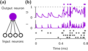
In SNNs, the input current is typically generated by synaptic currents triggered by the arrival of presynaptic spikes $S_{j}^{(l)}(t)$. When working with differential equations, it is convenient to denote a spike train $S_{j}^{(l)}(t)$ as a sum of Dirac delta functions $S_{j}^{(l)}(t)=\sum_{s\in C_{j}^{(l)}}\delta(t-s)$ where $s$ runs over the firing times $C_{j}^{(l)}$ of neuron $j$ in layer $l$.

Synaptic currents follow specific temporal dynamics themselves. A common first-order approximation is to model their time course as an exponentially decaying current following each presynaptic spike. Moreover, we assume that synaptic currents sum linearly. The dynamics of these operations are given by

$$\frac{\mathrm{d}I_{i}^{(l)}}{\mathrm{d}t}=-\underbrace{\frac{I_{i}^{(l)}(t)}{\tau_{\mathrm{syn}}}}_{\text{exp. decay}}+\underbrace{\sum_{j}W_{ij}^{(l)}S_{j}^{(l-1)}(t)}_{\mathrm{feed-forward}}+\underbrace{\sum_{j}V_{ij}^{(l)}S_{j}^{(l)}(t)}_{\mathrm{recurrent}}$$ (2)

where the sum runs over all presynaptic neurons $j$ and $W_{ij}^{(l)}$ are the corresponding afferent weights from the layer below. Further, the $V_{ij}^{(l)}$ correspond to explicit recurrent connections within each layer. Because of this property we can simulate a single LIF neuron with two linear differential equations whose initial conditions change instantaneously whenever a spike occurs. Through this property, we can incorporate the reset term in Equation (1) through an extra term that instantaneously decreases the membrane potential by the amount $(\vartheta-U_{\mathrm{rest}})$ whenever the neuron emits a spike:

$$\frac{\mathrm{d}U_{i}^{(l)}}{\mathrm{d}t}=-\frac{1}{\tau_{\mathrm{mem}}}\left((U_{i}^{(l)}-U_{\mathrm{rest}})+RI_{i}^{(l)}\right)+S_{i}^{(l)}(t)(U_{\mathrm{rest}}-\vartheta)$$ (3)

It is customary to approximate the solutions of Equations (2) and (3) numerically in discrete time and to express the output spike train $S_{i}^{(l)}[n]$ of neuron $i$ in layer $l$ at time step $n$ as a nonlinear function of the membrane voltage $S_{i}^{(l)}[n]\equiv\Theta(U_{i}^{(l)}[n]-\vartheta)$ where $\Theta$ denotes the Heaviside step function and $\vartheta$ corresponds to the firing threshold. Without loss of generality, we set $U_{\mathrm{rest}}=0$, $R=1$, and $\vartheta=1$. When using a small simulation time step $\Delta_{t}>0$, Equation (2) is well approximated by

$$I_{i}^{(l)}[n+1]=\alpha I_{i}^{(l)}[n]+\sum_{j}W_{ij}^{(l)}S_{j}^{(l)}[n]+\sum_{j}V_{ij}^{(l)}S_{j}^{(l)}[n]$$ (4)

with the decay strength $\alpha\equiv\exp\left(-\frac{\Delta_{t}}{\tau_{\mathrm{syn}}}\right)$. Note that $0<\alpha<1$ for finite and positive $\tau_{\mathrm{syn}}$. Moreover, $S_{j}^{(l)}[n]\in\{0,1\}$. We use $n$ to denote the time step to emphasize the discrete dynamics. We can now express Equation (3) as

$$U_{i}^{(l)}[n+1]=\beta U_{i}^{(l)}[n]+I_{i}^{(l)}[n]-S_{i}^{(l)}[n]$$ (5)

with $\beta\equiv\exp\left(-\frac{\Delta_{t}}{\tau_{\mathrm{mem}}}\right)$.

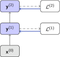
Equations (4) and (5) characterize the dynamics of a RNN. Specifically, the state of neuron $i$ is given by the instantaneous synaptic currents $I_{i}$ and the membrane voltage $U_{i}$ (Box. II). The computations necessary to update the cell state can be unrolled in time as is best illustrated by the computational graph (Figure 2).

Figure 2: Illustration of the computational graph of a SNN in discrete time. Time steps flow from left to right. Input spikes $\mathbf{S}^{(0)}$ are fed into the network from the bottom and propagate upwards to higher layers. The synaptic currents $\mathbf{I}$ are decayed by $\alpha$ in each time step and fed into the membrane potentials $\mathbf{U}$. The $\mathbf{U}$ are similarly decaying over time as characterized by $\beta$. Spike trains $\mathbf{S}$ are generated by applying a threshold nonlinearity to the membrane potentials $\mathbf{U}$ in each time step. Spikes causally affect the network state (red connections). First, each spike causes the membrane potential of the neuron that emits the spike to be reset. Second, each spike may be communicated to the same neuronal population via recurrent connections $\mathbf{V}^{(1)}$. Finally, it may also be communicated via $\mathbf{W}^{(2)}$ to another downstream network layer or, alternatively, a readout layer on which a cost function is defined.

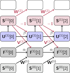
We have now seen that SNNs constitute a special case of RNNs. However, so far we have not explained how their parameters are set to implement a specific computational function. This is the focus of the rest of this article, in which we present a variety of learning algorithms that systematically change the parameters towards implementing specific functionalities.

III Methods for training RNNs

Powerful machine learning methods are able to train RNNs for a variety of tasks ranging from time series prediction, to language translation, to automatic speech recognition [1]. In the following, we discuss the most common methods before analyzing their applicability to SNNs.

There are several stereotypical ingredients that define the training process. The first ingredient is a cost or loss function which is minimized when the network’s response corresponds to the desired behavior. In time series prediction, for example, this loss could be the squared difference between the predicted and the true value. The second ingredient is a mechanism that updates the network’s weights to minimize the loss. One of the simplest and most powerful mechanisms to achieve this is to perform gradient descent on the loss function. In network architectures with hidden units (i.e. units whose activity affect the loss indirectly through other units) the parameter updates contain terms relating to the activity and weights of the downstream units they project to. Gradient-descent learning solves this credit assignment problem by providing explicit expressions for these updates through the chain rule of derivatives. As we will now see, the learning of hidden unit parameters depends on an efficient method to compute these gradients. When discussing these methods, we distinguish between solving the spatial credit assignment problem which affects multi-layer perceptrons (MLPs) and RNNs in the same way and the temporal credit assignment problem which only occurs in RNNs. We now discuss common algorithms which provide both types of credit assignment.

III-A Spatial credit assignment

To train MLPs, credit or blame needs to be assigned spatially across layers and their respective units. This spatial credit assignment problem is solved most commonly by the backpropagation (BP) of error algorithm (Box. III-A). In its simplest form, this algorithm propagates errors “backwards” from the output of the network to upstream neurons. Using BP to adjust hidden layer weights ensures that the weight update will reduce the cost function for the current training example, provided the learning rate is small enough. While this theoretical guarantee is desirable, it comes at the cost of certain communication requirements — namely that gradients have to be communicated back through the network — and increased memory requirements as the neuron states need to be kept in memory until the errors become available. [tbhp] The Gradient Backpropagation Rule for Neural Networks The task of learning is to minimize a cost function $\mathcal{L}$ over the entire dataset. In a neural network, this can be achieved by gradient descent, which modifies the network parameters $\mathbf{W}$ in the direction opposite to the gradient: $$\begin{split}W_{ij}\leftarrow W_{ij}-\eta\Delta W_{ij},&\text{where }\Delta W_{ij}=\frac{\partial\mathcal{L}}{\partial W_{ij}}=\frac{\partial\mathcal{L}}{\partial y_{i}}\frac{\partial y_{i}}{\partial a_{i}}\frac{\partial a_{i}}{\partial W_{ij}}\end{split}$$ with $a_{i}=\sum_{j}W_{ij}x_{j}$ the total input to the neuron, $y_{i}$ is the output of neuron $i$, and $\eta$ a small learning rate. The first term is the error of neuron $i$ and the second term reflects the sensitivity of the neuron output to changes in the parameter. In multilayer networks, gradient descent is expressed as the BP of the errors starting from the prediction (output) layer to the inputs. Using superscripts $l=0,...,L$ to denote the layer ($0$ is input, $L$ is output): $$\frac{\mathrm{\partial}}{\mathrm{\partial}W^{(l)}_{ij}}\mathcal{L}=\delta_{i}^{(l)}y^{(l-1)}_{j},\text{ where }\delta_{i}^{(l)}=\sigma^{\prime}\left(a_{i}^{(l)}\right)\sum_{k}\delta_{k}^{(l+1)}W_{ik}^{\top,(l)},$$ (6) where $\sigma^{\prime}$ is the derivative of the activation function, and $\delta_{i}^{(L)}=\frac{\partial\mathcal{L}}{\partial y_{i}^{(L)}}$ is the error of output neuron $i$ and $y_{i}^{(0)}=x_{i}$ and $\top$ indicates the transpose.
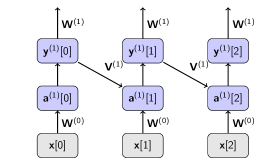
“Unrolled” RNN This update rule is ubiquitous in deep learning and known as the gradient BP algorithm [1]. Learning is typically carried out in forward passes (evaluation of the neural network activities) and backward passes (evaluation of $\delta$s). The same rule can be applied to RNNs. In this case the recurrence is “unrolled” meaning that an auxiliary network is created by making copies of the network for each time step. The unrolled network is simply a deep network with shared feedforward weights $\mathbf{W}^{(l)}$ and recurrent weights $\mathbf{V}^{(l)}$, on which the standard BP applies: $$\begin{split}\Delta{W_{ij}^{(l)}}&\propto\frac{\mathrm{\partial}}{\mathrm{\partial}W^{(l)}_{ij}}\mathcal{L}[n]=\sum_{m=0}^{t}\delta_{i}^{(l)}[m]y^{(l-1)}_{j}[m],\text{ and }\Delta{V_{ij}^{(l)}}\propto\frac{\mathrm{\partial}}{\mathrm{\partial}V^{(l)}_{ij}}\mathcal{L}[n]=\sum_{m=1}^{t}\delta_{i}^{(l)}[s]y^{(l)}_{j}[m-1]\\ \delta_{i}^{(l)}[n]&=\sigma^{\prime}\left(a_{i}^{(l)}[n]\right)\left(\sum_{k}\delta_{k}^{(l+1)}[n]W_{ik}^{\top,l}+\sum_{k}\delta_{k}^{(l)}[n+1]V_{ik}^{\top,l}\right),\end{split}$$ (7) Applying BP to an unrolled network is referred to as backpropagation through time (BPTT).

III-B Temporal credit assignment

When training RNNs, we also have to consider temporal interdependencies of network activity. This requires solving the temporal credit assignment problem (Fig. 2). There are two common methods to achieve this:

1. The “backward” method: This method applies the same strategies as with spatial credit assignment by “unrolling” the network in time (Box. III-A). Backpropagation through time (BPTT) solves the temporal credit assignment problem by back-propagating errors through the unrolled network. This method works backward through time after completing a forward pass. The use of standard BP on the unrolled network directly enables the use of autodifferentiation tools offered in modern machine learning toolkits [3, 13].

2. The forward method: In some situations, it is beneficial to propagate all necessary information for gradient computation forward in time [14]. This formulation is achieved by computing the gradient of a cost function $\mathcal{L}[n]$ and maintaining the recursive structure of the RNN. For example, the “forward gradient” of the feed-forward weight $\mathbf{W}$ becomes:

   $$\begin{split}\Delta{W_{ij}^{m}}&\propto\frac{\partial\mathcal{L}[n]}{\partial W_{ij}^{m}}=\sum_{k}\frac{\partial\mathcal{L}[n]}{\partial y_{k}^{(L)}[n]}P_{ijk}^{L,m}[n],\text{ with }P_{ijk}^{(l,m)}[n]=\frac{\partial}{\partial W_{ij}^{m}}y_{k}^{(l)}[n]\\ P_{ijk}^{(l,m)}[n]&=\sigma^{\prime}(a^{(l)}_{k}[n])\left(\sum_{j^{\prime}}V_{ij^{\prime}}^{(l)}P_{ijj^{\prime}}^{(l,m)}[n-1]+\sum_{j^{\prime}}W_{ij^{\prime}}^{(l)}P_{ijj^{\prime}}^{(l-1,m)}[n-1]+\delta_{lm}y_{i}^{(l-1)}[n-1]\right).\\ \end{split}$$ (8)

   Gradients with respect to recurrent weights $V_{ij}^{(l)}$ can be computed in a similar fashion [14].

The backward optimization method is generally more efficient in terms of computation, but requires maintaining all the inputs and activations for each time step. Thus, its space complexity for each layer is $O(NT)$, where $N$ is the number of neurons per layer and $T$ is the number of time steps. On the other hand, the forward method requires maintaining variables $P_{ijk}^{(l,m)}$, resulting in a $O(N^{3})$ space complexity per layer. While $O(N^{3})$ is not a favorable scaling compared to $O(NT)$ for large $N$, simplifications of the computational graph can reduce the memory complexity of the forward method to $O(N^{2})$ [15, 2], or even $O(N)$[4]. These simplifications also reduce the computational complexity, rendering the scaling of forward algorithms comparable or better than BPTT. Such simplifications are at the core of several successful approaches which we will describe in Sec. V. Furthermore, the forward method is more appealing from a biological point of view, since the learning rule can be made consistent with synaptic plasticity in the brain and “three-factor” rules, as discussed in Section V-B.

In summary, efficient algorithms to train RNNs exist. We will now focus on training SNNs.

IV Credit assignment with spiking neurons: Challenges and solutions

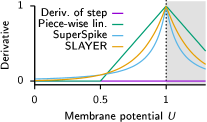
So far we have discussed common algorithmic solutions to training RNNs. Before these solutions can be applied to SNNs, however, two key challenges need to be overcome. The first challenge concerns the non-differentiability of the spiking nonlinearity. Equations (7) and (8) reveal that the expressions for both the forward and the backward learning methods contain the derivative of the neural activation function $\sigma^{\prime}\equiv\frac{\partial y_{i}^{(l)}}{\partial a_{i}^{(l)}}$ as a multiplicative factor. For a spiking neuron, however, we have $S(U(t))=\Theta(U(t)-\vartheta)$, whose derivative is zero everywhere except at $U=\vartheta$, where it is ill defined (Fig. 3).

This all-or-nothing behavior of the binary spiking nonlinearity stops gradients from “flowing” and makes LIF neurons unsuitable for gradient based optimization. The same issue occurs in binary neurons and some of the solutions proposed here are inspired by the methods first developed in binary networks [16, 17].

Figure 3: Commonly used surrogate derivatives. The step function has zero derivative (violet) everywhere except at 0 where it is ill defined. Examples of surrogate derivatives which have been used to train SNNs. Green: Piece-wise linear [18, 3, 19]. Blue: Derivative of a fast sigmoid [2]. Yellow: Exponential [13]. Note that the axes have been rescaled on a per-function-basis for illustration purposes.

The second challenge concerns the implementation of the optimization algorithm itself. Standard BP can be expensive in terms of computation, memory and communication, and may be poorly suited to the constraints dictated by the hardware that implements it (e.g. a computer, a brain, or a neuromorphic device). Processing in dedicated neuromorphic hardware and, more generally, non-von Neumann computers may have specific locality requirements (Box. V-A) that can complicate matters. On such hardware, the forward approach may therefore be preferable. In practice, however, the scaling of both methods ($O(N^{3})$ and $O(NT)$) has proven unsuitable for many SNN models. For example, the size of the convolutional SNN models trained with BPTT for gesture classification [20] are GPU memory bounded. Additional simplifying approximations that reduce the complexity of the forward method will be discussed below. In the following sections, we describe approximate solutions to these challenges that make learning in SNNs more tractable.

To overcome the first challenge in training SNNs, which is concerned with the discontinuous spiking nonlinearity, several approaches have been devised with varying degrees of success. The most common approaches can be coarsely classified into the following categories: i) resorting to entirely biologically inspired local learning rules for the hidden units, ii) translating conventionally trained “rate-based” neural networks to SNNs, iii) smoothing the network model to be continuously differentiable, or iv) defining a surrogate gradient (SG) as a continuous relaxation of the real gradients. Approaches pertaining biologically motivated local learning rules (i) and network translation (ii) have been reviewed extensively elsewhere [21, 5]. In this article, we therefore focus on the latter two supervised approaches (iii & iv) which we will refer to as the “smoothed” and the SG approach. First, we review existing literature on common “smoothing” approaches before turning to an in-depth discussion of how to build functional SNNs using SG methods.

IV-A Smoothed spiking neural networks

The defining characteristic of smoothed SNNs is that their formulation ensures well-behaved gradients which are directly suitable for optimization. Smooth models can be further categorized into (1) soft nonlinearity models, (2) probabilistic models, for which gradients are only well defined in expectation, or models which either rely entirely on (3) rate or (4) single-spike temporal codes.

IV-A1 Gradients in soft nonlinearity models

This approach can in principle be applied directly to all spiking neuron models which explicitly include a smooth spike generating process. This includes, for instance, the Hodgkin-Huxley, Morris-Lecar, and FitzHugh-Nagumo models [12]. In practice this approach has only been applied successfully by Huh and Sejnowski [22] using an augmented integrate-and-fire model in which the binary spiking nonlinearity was replaced by a continuous-valued gating function. The resulting network constitutes a RCNN which can be optimized using standard methods of BPTT or real-time recurrent learning (RTRL). Importantly, the soft threshold models compromise on one of the key features of SNN, namely the binary spike propagation.

IV-A2 Gradients in probabilistic models

Another example for smooth models are binary probabilistic models. In simple terms, stochasticity effectively smooths out the discontinuous binary nonlinearity which makes it possible to define a gradient on expectation values. Binary probabilistic models have been objects of extensive study in the machine learning literature mainly in the context of (restricted) Boltzmann machines [23]. Similarly, the propagation of gradients has been studied for binary stochastic models [17].

Probabilistic models are practically useful because the log-likelihood of a spike train is a smooth quantity which can be optimized using gradient descent [24]. Although this insight was first discovered in networks without hidden units, the same ideas were later extended to multi-layer networks [25]. Similarly, Guerguiev et al. [26] used probabilistic neurons to study biologically plausible ways of propagating error or target signals using segregated dendrites (see Section V-A). In a similar vein, variational learning approaches were shown to be capable of learning useful hidden layer representations in SNNs [27, 28, 29]. However, the injected noise necessary to smooth out the effect of binary nonlinearities often poses a challenge for optimization [28]. How noise, which is found ubiquitously in neurobiology, influences learning in the brain, remains an open question.

IV-A3 Gradients in rate-coding networks

Another common approach to obtain gradients in SNNs is to assume a rate-based coding scheme. The main idea is that spike rate is the underlying information-carrying quantity. For many plausible neuron models, the supra-threshold firing rate depends smoothly on the neuron input. This input-output dependence is captured by the so-called f-I curve of a neuron. In such cases, the derivative of the f-I curves is suitable for gradient-based optimization.

There are several examples of this approach. For instance, Hunsberger and Eliasmith [30] as well as Neftci et al. [31] used an effectively rate-coded input scheme to demonstrate competitive performance on standard machine learning benchmarks such as CIFAR10 and MNIST. Similarly Lee et al. [32] demonstrated deep learning in SNNs by defining partial derivatives on low-pass filtered spike trains.

Rate-based approaches can offer good performance, but they may be inefficient. On the one hand, precise estimation of firing rates requires averaging over a number of spikes. Such averaging requires either relatively high firing rates or long averaging times because several repeats are needed to average out discretization noise. This problem can be partially addressed by spatial averaging over large populations of spiking neurons. However, this may require the use of larger neuron numbers.

Finally, the distinction between rate-coding and probabilistic networks can be blurry since many probabilistic network implementations use rate-coding at the output level. Both types of models are differentiable, but for different reasons: Probabilistic models are based on a firing probability densities [24]. Importantly, the firing probability of a neuron is a continuous function. Although measuring probability changes requires “trial averaging” over several samples, it is the underlying continuity of the probability density which formally allows to define differential improvements and thus to derive gradients. By exploiting this feature, probabilistic models have been used to learn precise output spike timing [24, 25]. In contrast, deterministic networks always emit a fixed integer number of spikes for a given input. To nevertheless get at a notion of differential improvement, one may consider the number of spikes over a given time interval within single trials. When averaging over sufficiently large intervals, the resulting firing rates behave as a quasi continuous function of the input current. This smooth input output relationship is captured by the neuronal f-I curve which can be used for optimization [30, 31]. Operating at the level of rates, however, comes at the expense temporal precision.

IV-A4 Gradients in single-spike-timing-coding networks

In an effort to optimize SNNs without potentially harmful noise injection and without reverting to a rate-based coding scheme, several studies have considered the outputs of neurons in SNNs to be a set of firing times. In such a temporal coding setting, individual spikes could carry significantly more information than rate-based schemes that only consider the total number of spikes in an interval.

The idea behind training temporal coding networks was pioneered in SpikeProp [33]. In this work the analytic expressions of firing times for hidden units were linearized, allowing to analytically compute approximate hidden layer gradients. More recently, a similar approach without the need for linearization was used in [34] where the author computed the spike timing gradients explicitly for non-leaky integrate-and-fire neurons. Intriguingly, the work showed competitive performance on conventional networks and benchmarks.

Although the spike timing formulation does in some cases yield well-defined gradients, it may suffer from certain limitations. For instance, the formulation of SpikeProp [33] required each hidden unit to emit exactly one spike per trial, because it is impossible to define firing time for quiescent units. Ultimately, such a non-quiescence requirement could be at conflict with power-efficiency for which it is conceivably beneficial to, for instance, only have a subset of neurons active for any given task.

IV-B Surrogate gradients

SG methods provide an alternative approach to overcoming the difficulties associated with the discontinuous nonlinearity. Moreover, they hold opportunities to reduce the potentially high algorithmic complexity associated with training SNNs. Their defining characteristic is that instead of changing the model definition as in the smoothed approaches, a SG is introduced. In the following we make two distinctions. We first consider SGs which constitute a continuous relaxation of the non-smooth spiking nonlinearity for purposes of numerical optimization (Fig. 4). Such SGs do not explicitly change the optimization algorithm itself and can be used, for instance, in combination with BPTT. Further, we also consider SGs with more profound changes that explicitly affect locality of the underlying optimization algorithms themselves to improve the computational and/or memory access overhead of the learning process. One example of this approach that we will discuss involves replacing the global loss by a number of local loss functions. Finally, the use of SGs allows to efficiently train SNNs end-to-end without the need to specify which coding scheme is to be used in the hidden layers.

Figure 4: Example of SG for a SNN classifier. (a) Value of the loss function (gray) of an SNN classifier along an interpolation path over the hidden layer parameters $\mathbf{W}^{(1)}$. Specifically, we linearly interpolated between the random initial and final (post-optimization) weight matrices of the hidden layer inputs $\mathbf{W}^{(1)}$ (network details: 2 input, 2 hidden, and 2 output units trained on a binary classification task). Note that the loss function (gray) displays characteristic plateaus with zero gradient which are detrimental for numerical optimization. (b) Norm of hidden layer (surrogate) gradients in arbitrary units along the interpolation path. To perform numerical optimization in this network we constructed a SG (violet) which, in contrast to the true gradient (gray), is non-zero. Note that we obtained the “true gradient” via the finite differences method which in itself is an approximation. Importantly, the SG approximates the true gradient, but retains favorable properties for optimization, i.e. continuity and finiteness. The SG can be thought of as the gradient of a virtual surrogate loss function (violet curve in (a); obtained by numerical integration of the SG and scaled to match loss at initial and final point). This surrogate loss remains virtual because it is generally not computed explicitly. In practice, suitable SGs are obtained directly from the gradients of the original network through sensible approximations. This is a key difference with respect to some other approaches [22] in which the entire network is replaced explicitly by a surrogate network on which gradient descent can be performed using its true gradients.

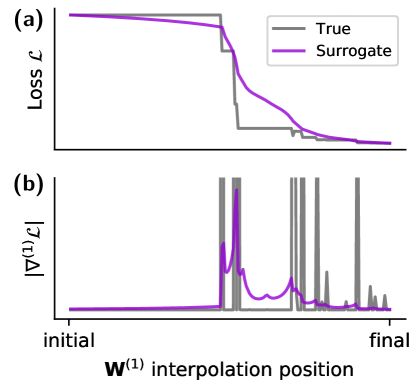
Like standard gradient-descent, SG learning can deal with the spatial and temporal credit assignment problem by either BPTT or by forward methods, e.g. through the use of eligibility traces (see Section III-B for details). Alternatively, additional approximations can be introduced which may offer advantages specifically for hardware implementations. In the following, we briefly review existing work relying on SG methods before turning to a more in-depth treatment of the underlying principles and capabilities.

IV-B1 Surrogate derivatives for spiking nonlinearity

A set of works have used SG to specifically overcome the challenge of the discontinuous spiking nonlinearity. In these works, typically a standard algorithm such as BPTT is used with one minor modification: within the algorithm each occurrence of the derivative of the spiking nonlinearity is replaced by the derivative of a smooth function. Implementing these approaches is straight-forward in most auto-differentiation-enabled machine learning toolkits.

One of the first uses of such a SG is described in Bohte [19] where the derivative of a spiking neuron non-linearity was approximated by the derivative of a truncated quadratic function, thus resulting in a rectifying linear unit (ReLU) as surrogate derivative (Fig. 3). This is similar in flavor to the solution proposed to optimize binary neural networks [16]. The same idea underlies the training of large-scale convolutional networks with binary activations on classification problems using neuromorphic hardware [18]. Zenke and Ganguli [2] proposed a three factor online learning rule using a fast sigmoid to construct a SG. Shrestha and Orchard [13] used an exponential function and reported competitive performance on a range of neuromorphic benchmark problems. Additionally, O’Connor et al. [35] described a spike-based encoding method inspired by Sigma-Delta modulators. They used their method to approximately encode both the activations and the errors in standard feedforward artificial neural networks (ANNs), and apply standard backpropagation on these sparse approximate encodings.

Surrogate derivatives have also been used to train spiking RCNNs where dynamical recurrence arises due to the use of LIF neurons as well as due to recurrent synaptic connections. Recently, Bellec et al. [3] successfully trained RCNNs with slow temporal neuronal dynamics using a piecewise linear surrogate derivative. Encouragingly, the authors found that such networks can perform on par with conventional long short-term memory (LSTM) networks. Similarly, Woźniak et al. [36] reported competitive performance on a series of temporal benchmark datasets.

In summary, a plethora of studies have constructed SG using different nonlinearities and trained a diversity of SNN architectures. These nonlinearties, however, have a common underlying theme. All functions are nonlinear and monotonically increasing towards the firing threshold (Fig. 3). While a more systematic comparison of different surrogate nonlinearities is still pending, overall the diversity found in the present literature suggests that the success of the method is not crucially dependent on the details of the surrogate used to approximate the derivative.

IV-B2 Surrogate gradients affecting locality of the update rules

The majority of studies discussed in the previous section introduced a surrogate nonlinearity to prevent gradients from vanishing (or exploding), but by relying on methods such as BPTT, they did not explicitly affect the structural properties of the learning rules. There are, however, training approaches for SNNs which introduce more far-reaching modifications which may completely alter the way error signals or target signals are propagated (or generated) within the network. Such approaches are typically used in conjunction with the aforementioned surrogate derivatives. There are two main motivations for such modifications which are typically linked to physical constraints that make it impossible to implement the “correct” gradient descent algorithm. For instance, in neurobiology biophysical constraints make it impossible to implement BPTT without further approximations. Studies interested in how the brain could solve the credit assignment problem focus on how simplified “local” algorithms could achieve similar performance while adhering to the constraints of the underlying biological wetware (Box. V-A). Similarly, neuromorphic hardware may pose certain constraints with regard to memory or communications which impede the use of BPTT and call for simpler and often more local methods for training on such devices.

As training SNNs using SGs advances to deeper architectures, it is foreseeable that additional problems, similar to the ones encountered in ANNs, will arise. For instance, several approaches currently rely on SGs derived from sigmoidal activation functions (Fig. 3). However, the use of sigmoidal activation functions is implicated with vanishing gradient problems. Another set of challenges which may well need tackling in the future could be linked to the bias which SGs introduce into the learning dynamics.

In the following Applications Section, we will review a selection of promising SG approaches which introduce far larger deviations from the “true gradients” and still allow for learning at a greatly reduced complexity and computational cost.

(a) BP

(b) FA

(c) DFA

(d) Local Errors

Figure 5: Strategies for relaxing gradient BP requirements. Dashed lines indicate fixed, random connections. (a) BP propagates errors through each layer using the transpose of the forward weights by alternating forward and backward passes. (b) Feedback Alignment [37] replaces the transposed matrix with a random one. (c) Direct Feedback Alignment [38] directly propagates the errors from the top layer to the hidden layers. (d) Local errors [29] uses a fixed, random, auxiliary cost function at each layer.

V Applications

In this section, we present a selection of illustrative applications of smooth or SGs to SNNs which exploit both the internal continuous-time dynamics of the neurons and their event-driven nature. The latter allows a network to remain quiescent until incoming spikes trigger activity.

V-A Feedback alignment and random error backpropagation

One family of algorithms that relaxes some of the requirements of BP are feedback alignment or, more generally, random BP algorithms [37, 39, 38]. These are approximations to the gradient BP rule that side-step the non-locality problem by replacing weights in the BP rule with random ones (Fig. 5b): $\delta_{i}^{(l)}=\sigma^{\prime}\left(a_{i}^{(l)}\right)\sum_{k}\delta_{k}^{(l+1)}G_{ki}^{(l)},$ where $\mathbf{G}^{(}l)$ is a fixed, random matrix with the same dimensions as ${\bf W}$. The replacement of $\mathbf{W}^{\top,(l)}$ with a random matrix $\mathbf{G}^{(l)}$ breaks the dependency of the backward phase on $\mathbf{W}^{(l)}$, enabling the rule to be more local. One common variation is to replace the entire backward propagation by a random propagation of the errors to each layer (Fig. 5c) [38]: $\delta_{i}^{(l)}=\sigma^{\prime}\left(a_{i}^{(l)}\right)\sum_{k}\delta^{(L)}_{k}H_{ki}^{(l)},$ where $\mathbf{H}^{(l)}$ is a fixed, random matrix with appropriate dimensions.

Random BP approaches lead to remarkably little loss in classification performance on some benchmark tasks. Although a general theoretical understanding of random BP is still a subject of intense research, simulation studies have shown that, during learning, the network adjusts its feed-forward weights such that they partially align with the (random) feedback weights, thus permitting them to convey useful error information [37]. Building on these findings, an asynchronous spike-driven adaptation of random BP using local synaptic plasticity rules with the dynamics of spiking neurons was demonstrated in [31]. To obtain the SGs, the authors approximated the derivative of the neural activation function using a symmetric function that is zero everywhere except in the vicinity of zero, where it is constant. The derivative of this function exists and is piecewise constant. Networks using this learning rule performed remarkably well, and were shown to operate continuously and asynchronously without the alternation between forward and backward passes that is necessary in BP. One important limitation with random BP applied to SNNs was that the temporal dynamics of the neurons and synapses was not taken into account in the gradients. The following rule, SuperSpike solves this problem.

[tbhp] Local models of computation Locality of computations is characterized by the set variables available to the physical processing elements, and depends on the computational substrate. To illustrate the concept of locality, we assume two neurons, $A$ and $B$, and would like Neuron $A$ to implement a function on domain $D$ defined as: $$\begin{split}D&=D_{loc}\cup D_{nloc},\text{where }D_{loc}=\{W_{BA},S_{A}(t),U_{A}(t)\}\\ \text{ and }D_{nloc}&=\{S_{B}(t-T),U_{B}\}.\end{split}$$ Here, $S^{B}(t-T)$ refers to the output of neuron $B$ $T$ seconds ago, $U_{A}$, $U_{B}$ are the respective membrane potentials, and $W_{BA}$ is the synaptic weight from $B$ to $A$. Variables under $D_{loc}$ are directly available to Neuron A and are thus local to it. On the other hand, variable $S^{B}(t-T)$ is temporally non-local and $U_{B}$ is spatially non-local to neuron $A$. Non-local information can be transmitted through special structures, for example dedicated encoders and decoders for $U_{B}$ and a form of working memory (WM) for $S_{B}(t-T)$. Although locality in a model of computation can make its use challenging, it enables massively parallel computations with dynamical interprocess communications.

V-B Supervised learning with local three factor learning rules

SuperSpike is a biologically plausible three factor learning rule. In contrast to many existing three factor rules which fall into the category of “smoothed approaches” [24, 25, 26, 27, 28, 29], SuperSpike is a SG approach which combines several approximations to render it more biologically plausible [2]. Although the underlying motivation of the study is geared toward a deeper understanding of learning in biological neural networks, the learning rule may prove interesting for hardware implementations because it does not rely on BPTT. Specifically, the rule uses synaptic eligibility traces to solve the temporal credit assignment problem.

We now provide a short account on why SuperSpike can be seen as one of the forward-in-time optimization procedures. SuperSpike was derived for temporal supervised learning tasks in which a given output neuron learns to spike at predefined times. To that end, SuperSpike minimizes the van Rossum distance with kernel $\epsilon$ between a set of output spike train $S_{k}(t)$ and their corresponding target spike trains $S_{k}^{*}(t)$

$$\mathcal{L}=\frac{1}{2}\int_{-\infty}^{t}\mathcal{L}(s)~{}ds=\frac{1}{2}\int_{-\infty}^{t}\left(\epsilon\ast(S_{k}(s)-S_{k}^{*}(s))\right)^{2}ds\approx\frac{1}{2}\sum_{n}\left(\epsilon\ast(S_{k}[n]-S_{k}^{*}[n])\right)^{2}$$ (9)

where the last approximation corresponds to transitioning to discrete time. To perform online gradient descent, we need to compute the gradients of $\mathcal{L}[n]$. Here we first encounter the derivative $\frac{\partial}{\partial W_{ij}}\epsilon\ast S_{k}[n]$. Because the (discrete) convolution is a linear operator, this expression simplifies to $\epsilon\ast\frac{\partial S_{k}[n]}{\partial W_{ij}}$. In SuperSpike $\epsilon$ is implemented as a dynamical system (see [2] for details). To compute derivatives of the neuron’s output spiketrain of the form $\frac{\partial S_{i}[n]}{\partial W_{ij}}$ we differentiate the network dynamics (Equations (4) and (5)) and obtain

$$\frac{\partial S_{k}[n+1]}{\partial W_{ij}} = \Theta^{\prime}(U_{k}[n+1]-\vartheta)\left[\frac{\partial U_{k}[n+1]}{\partial W_{ij}}\right]$$ (10)

$$\frac{\partial U_{k}[n+1]}{\partial W_{ij}} = \beta\frac{\partial U_{k}[n]}{\partial W_{ij}}+\frac{\partial I_{k}[n]}{\partial W_{ij}}-\frac{\partial S_{k}[n]}{\partial W_{ij}}$$ (11)

$$\frac{\partial I_{k}[n+1]}{\partial W_{ij}} = \alpha\frac{\partial I_{k}[n]}{\partial W_{ij}}+S_{j}[n]$$ (12)

The above equations define a dynamical system which, given the starting conditions $S_{k}[0]=U_{k}[0]=I_{k}[0]=0$, can be simulated online and forward in time to produce all relevant derivatives. Crucially, to arrive at useful SGs, SuperSpike makes two approximations. First, $\Theta^{\prime}$ is replaced by a smooth surrogate derivative $\sigma^{\prime}(U[n]-\vartheta)$ (cf. Fig. 3). Second, the reset term with the negative sign in Equation (11) is dropped, which empirically leads to better results. With these definitions in hand, the final weight updates are given by

$$\Delta W_{ij}[n]\propto e_{i}[n]\epsilon\ast\left[\sigma^{\prime}(U_{k}[n])\frac{\partial U_{k}[n]}{\partial W_{ij}}\right]$$ (13)

where $e_{i}[n]\equiv\epsilon\ast(S_{i}-S^{*}_{i})$. These weight updates depend only on local quantities (Box. V-A).

Above, we have considered a simple two-layer network (cf. Fig. 2) without recurrent connections. If we were to apply the same strategy to compute updates in a RCNN or a network with an additional hidden layer, the equations would become more complicated and non-local. SuperSpike applied to multi-layer networks sidesteps this issue by propagating error signals from the output layer directly to the hidden units as in random BP (cf. Section V-A; Fig. 5c; [37, 39, 38]). Thus, SuperSpike achieves temporal credit assignment by propagating all relevant quantities forward in time, while it relies on random BP to perform spatial credit assignment.

While the work by Zenke and Ganguli [2] was centered around feed-forward networks, Bellec et al. [15] show that similar biologically plausible three factors rule can also be used to train RCNN efficiently.

V-C Learning using local errors

In practice, the performance of SuperSpike does not scale favorably for large multilayer networks. The scalability of SuperSpike can be improved by introducing local errors, as described here.

Figure 6: Deep Continuous Local Learning (DCLL) with spikes [4], applied to the event-based DVSGestures dataset. The feed-forward weights (green) of a three layer convolutional SNN are trained with SG using local errors generated using fixed random projections to a local classifier. Learning in DCLL scales linearly with the number of neurons thanks to local rate-based cost functions formed by spike-based basis functions. The circular arrows indicate recurrence due to the statefulness of the LIF dynamics (no recurrent synaptic connections were used here) and are not trained. This SNN outperforms BPTT methods [13], requiring fewer training iterations [4] compared to other approaches.

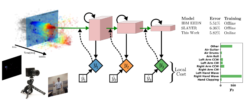
Multi-layer neural networks are hierarchical feature extractors. Through successive linear projections and point-wise non-linearities, neurons become tuned (respond most strongly) to particular spatio-temporal features in the input. While the best features are those that take into account the subsequent processing stages and which are learned to minimize the final error (as the features learned using BP do), high-quality features can also be obtained by more local methods. The non-local component of the weight update equation (Eq. (6)) is the error term $\delta_{i}^{(l)}[n]$. Instead of obtaining this error term through BP, we require that it be generated using information local to the layer. One way of achieving this is to define a layer-wise loss $\mathcal{L}^{(l)}({y}^{(l)}[n])$ and use this local loss to obtain the errors. In such a local learning setting, the local errors $\delta^{(l)}$ becomes:

$$\delta_{i}^{(l)}[n]=\sigma^{\prime}\left(a_{i}^{(l)}[n]\right)\frac{\mathrm{d}}{\mathrm{d}y_{i}^{(l)}[n]}\mathcal{L}^{(l)}(\mathbf{y}^{(l)}[n])\text{ where }\mathcal{L}^{(l)}(\mathbf{y}^{(l)}[n])\equiv\mathcal{L}(\mathbf{G}^{(l)}\mathbf{y}^{(l)}[n],\hat{\mathbf{y}}^{(l)}[n])$$ (14)

with $\hat{{\bf y}}^{(l)}[n]$ a pseudo-target for layer $l$, and ${\bf G}^{(l)}$ a fixed random matrix that projects the activity vector at layer $l$ to a vector having the same dimension as the pseudo-target. In essence, this formulation assumes that an auxiliary random layer is attached to layer $l$ and the goal is to modify $\mathbf{\bf W}^{(l)}$ so as to minimize the discrepancy between the auxiliary random layer’s output and the pseudo-target. The simplest choice for the pseudo-target is to use the top-layer target. This forces each layer to learn a set of features that are able to match the top-layer target after undergoing a fixed random linear projection. Each layer builds on the features learned by the layer below it, and we empirically observe that higher layers are able to learn higher-quality features that allow their random and fixed auxiliary layers to better match the target [40].

A related approach was explored with spiking neural networks [41], where separate networks provided high-dimensional temporal signals to improve learning. Local errors were recently used in SNNs in combination with the SuperSpike (cf. Section V-B) forward method to overcome the temporal credit assignment problem [4]. As in SuperSpike, the SNN model is simplified by using a feedforward structure, and omitting the refractory dynamics in the optimization. However, the cost function was defined to operate locally on the instantaneous rates of each layer. This simplification results in a forward method whose space complexity scales as $O(N)$ (instead of $O(N^{3})$ for the forward method, $O(N^{2})$ for SuperSpike, or $O(NT)$ for the backward method), while still making use of spiking neural dynamics. Thus the method constitutes a highly efficient synaptic plasticity rule for multi-layer SNNs. Furthermore, the simplifications enable the use of existing automatic differentiation methods in machine learning frameworks to systematically derive synaptic plasticity rules from task-relevant cost functions and neural dynamics (see [4] and included tutorials), making DCLL easy to implement. This approach was benchmarked on the DVS Gestures dataset (Fig. 6), and performs on par with standard BP or BPTT rules.

V-D Learning using gradients of spike times

Difficulties in training SNNs stem from the discrete nature of the quantities of interest such as the number of spikes in a particular interval. The derivatives of these discrete quantities are zero almost everywhere which necessitates the use of SG methods. Alternatively, we can choose to use spike-based quantities that have well defined, smooth derivatives. One such quantity is spike times. This capitalizes on the continuous-time nature of SNNs and results in highly sparse network activity as the emission time of even a single spike can encode significant information. Just as importantly, spike times are continuous quantities that can be made to depend smoothly on the neuron’s input. Working with spike times is thus a complementary approach to SG but which achieves the same goal: obtaining a smooth chain of derivatives between the network’s outputs and inputs. For this example, we use non-leaky integrate and fire neurons described by:

$$\frac{\mathrm{d}U_{i}}{\mathrm{d}t}=I_{i}\quad\text{with}\quad I_{i}=\sum\limits_{j}W_{ij}\sum\limits_{r}\Theta(t-t_{i}^{r})\exp\left(-(t-t_{i}^{r})\right)$$ (15)

where $t_{i}^{r}$ is the time of the $r^{\mathrm{th}}$ spike from neuron $j$, and $\Theta$ is the Heaviside step function.

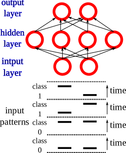
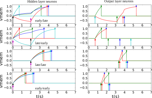
Consider the simple exclusive or (XOR) problem in the temporal domain: A network receives two spikes, one from each of two different sources. Each spike can either be “early” or “late”. The network has to learn to distinguish between the case in which the spikes are either both early or both late, and the case where one spike is early and the other is late (Fig. 7a). When designing a SNN, there is significant freedom in how the network input and output are encoded. In this case, we use a first-to-spike code in which we have two output neurons and the binary classification result is represented by the output neuron that spikes first. Figure 7b shows the network’s response after training (see [34] for details on the training process). For the first input class (early/late or late/early), one output neuron spikes first and for the other class (early/early or late/late), the other output neuron spikes first.

(a)

(b)

Figure 7: Temporal XOR problem. (a) An SNN with one hidden layer. Each input neuron emits one spike which can either be late or early resulting in four possible input patterns that should be classified into two classes. (b) For the four input spike patterns (one per row), the right plots show the membrane potentials of the two output neurons, while the left plots show the membrane potentials of the four hidden neurons. Arrows at the top of the plot indicate output spikes from the layer, while arrows at the bottom indicate input spikes. The output spikes of the hidden layer are the input spikes of the output layer. The classification result is encoded in the identity of the output neuron that spikes first.

.

VI Conclusion

We have outlined how SNNs can be studied within the framework of RNNs and discussed successful approaches for training them. We have specifically focused on SG approaches for two reasons: SG approaches are able to train SNNs to unprecedented performance levels on a range of real-world problems. This transition marks the beginning of an exciting time in which SNNs will become increasingly interesting for applications which were previously dominated by RNNs; SGs provide a framework that ties together ideas from machine learning, computational neurosciences, and neuromorphic computing. From the viewpoint of computational neuroscience, the approaches presented in this paper are appealing because several of them are related to “three-factor” plasticity rules which are an important class of rules believed to underlie synaptic plasticity in the brain. Finally, for the neuromorphic community, SG methods provide a way to learn under various constraints on communication and storage which makes SG methods highly relevant for learning on custom low-power neuromorphic devices.

The spectacular successes of modern ANNs were enabled by algorithmic and hardware advances that made it possible to efficiently train large ANNs on vast amounts of data. With temporal coding, SNNs are universal function approximators that are potentially far more powerful than ANNs with sigmoidal nonlinearities. Unlike large-scale ANNs, which had to wait for several decades until the necessary computational resources were available for training them, we currently have the necessary resources, whether in the form of mainstream compute devices such as CPUs or GPUs, or custom neuromorphic devices, to train and deploy large SNNs. The fact that SNNs are less widely used than ANNs is thus primarily due to the algorithmic issue of trainability. In this article, we have provided an overview of various exciting developments that are gradually addressing the issues encountered when training SNNs. Fully addressing these issues would have immediate and wide-ranging implications, both technologically, and in relation to learning in biological brains.

References

- Goodfellow et al. [2016] I. Goodfellow, Y. Bengio, and A. Courville, Deep learning. MIT press, 2016.
- Zenke and Ganguli [2018] F. Zenke and S. Ganguli, “SuperSpike: Supervised Learning in Multilayer Spiking Neural Networks,” Neural Computation, vol. 30, no. 6, pp. 1514–1541, Apr. 2018.
- Bellec et al. [2018] G. Bellec, D. Salaj, A. Subramoney, R. Legenstein, and W. Maass, “Long short-term memory and Learning-to-learn in networks of spiking neurons,” in Advances in Neural Information Processing Systems 31, S. Bengio, H. Wallach, H. Larochelle, K. Grauman, N. Cesa-Bianchi, and R. Garnett, Eds. Curran Associates, Inc., 2018, pp. 795–805.
- Kaiser et al. [2018] J. Kaiser, H. Mostafa, and E. Neftci, “Synaptic plasticity for deep continuous local learning,” arXiv preprint arXiv:1812.10766, 2018.
- Tavanaei et al. [2018] A. Tavanaei, M. Ghodrati, S. R. Kheradpisheh, T. Masquelier, and A. Maida, “Deep learning in spiking neural networks,” Neural Networks, Dec. 2018.
- Gütig [2014] R. Gütig, “To spike, or when to spike?” Current Opinion in Neurobiology, vol. 25, pp. 134–139, Apr. 2014.
- Memmesheimer et al. [2014] R.-M. Memmesheimer, R. Rubin, B. Ölveczky, and H. Sompolinsky, “Learning Precisely Timed Spikes,” Neuron, vol. 82, no. 4, pp. 925–938, May 2014.
- Anwani and Rajendran [2015] N. Anwani and B. Rajendran, “NormAD-normalized approximate descent based supervised learning rule for spiking neurons,” in Neural Networks (IJCNN), 2015 International Joint Conference on. IEEE, 2015, pp. 1–8.
- Gilra and Gerstner [2017] A. Gilra and W. Gerstner, “Predicting non-linear dynamics by stable local learning in a recurrent spiking neural network,” eLife Sciences, vol. 6, p. e28295, Nov. 2017. [Online]. Available: https://elifesciences.org/articles/28295
- Nicola and Clopath [2017a] W. Nicola and C. Clopath, “Supervised learning in spiking neural networks with FORCE training,” Nature Communications, vol. 8, no. 1, p. 2208, Dec. 2017.
- Boahen [2017] K. Boahen, “A neuromorph’s prospectus,” Computing in Science Engineering, vol. 19, no. 2, pp. 14–28, Mar. 2017.
- Gerstner et al. [2014] W. Gerstner, W. M. Kistler, R. Naud, and L. Paninski, Neuronal dynamics: From single neurons to networks and models of cognition. Cambridge University Press, 2014.
- Shrestha and Orchard [2018a] S. B. Shrestha and G. Orchard, “SLAYER: Spike Layer Error Reassignment in Time,” in Advances in Neural Information Processing Systems 31, S. Bengio, H. Wallach, H. Larochelle, K. Grauman, N. Cesa-Bianchi, and R. Garnett, Eds. Curran Associates, Inc., 2018, pp. 1419–1428.
- Williams and Zipser [1989] R. J. Williams and D. Zipser, “A learning algorithm for continually running fully recurrent neural networks,” Neural computation, vol. 1, no. 2, pp. 270–280, 1989.
- Bellec et al. [2019] G. Bellec, F. Scherr, E. Hajek, D. Salaj, R. Legenstein, and W. Maass, “Biologically inspired alternatives to backpropagation through time for learning in recurrent neural nets,” arXiv:1901.09049 [cs], Jan. 2019. [Online]. Available: http://arxiv.org/abs/1901.09049
- Courbariaux et al. [2016] M. Courbariaux, I. Hubara, D. Soudry, R. El-Yaniv, and Y. Bengio, “Binarized Neural Networks: Training Deep Neural Networks with Weights and Activations Constrained to +1 or -1,” arXiv:1602.02830 [cs], Feb. 2016, arXiv: 1602.02830.
- Bengio et al. [2013] Y. Bengio, N. Léonard, and A. Courville, “Estimating or Propagating Gradients Through Stochastic Neurons for Conditional Computation,” arXiv:1308.3432 [cs], Aug. 2013, arXiv: 1308.3432.
- Esser et al. [2016] S. K. Esser, P. A. Merolla, J. V. Arthur, A. S. Cassidy, R. Appuswamy, A. Andreopoulos, D. J. Berg, J. L. McKinstry, T. Melano, D. R. Barch, C. di Nolfo, P. Datta, A. Amir, B. Taba, M. D. Flickner, and D. S. Modha, “Convolutional networks for fast, energy-efficient neuromorphic computing,” Proc Natl Acad Sci U S A, vol. 113, no. 41, pp. 11 441–11 446, Oct. 2016.
- Bohte [2011] S. M. Bohte, “Error-Backpropagation in Networks of Fractionally Predictive Spiking Neurons,” in Artificial Neural Networks and Machine Learning – ICANN 2011, ser. Lecture Notes in Computer Science. Springer, Berlin, Heidelberg, Jun. 2011, pp. 60–68.
- Shrestha and Orchard [2018b] S. B. Shrestha and G. Orchard, “Slayer: Spike layer error reassignment in time,” arXiv preprint arXiv:1810.08646, 2018.
- Abbott et al. [2016] L. F. Abbott, B. DePasquale, and R.-M. Memmesheimer, “Building functional networks of spiking model neurons,” Nat Neurosci, vol. 19, no. 3, pp. 350–355, Mar. 2016.
- Huh and Sejnowski [2018] D. Huh and T. J. Sejnowski, “Gradient Descent for Spiking Neural Networks,” in Advances in Neural Information Processing Systems 31, S. Bengio, H. Wallach, H. Larochelle, K. Grauman, N. Cesa-Bianchi, and R. Garnett, Eds. Curran Associates, Inc., 2018, pp. 1440–1450.
- Ackley et al. [1985] D. Ackley, G. Hinton, and T. Sejnowski, “A learning algorithm for Boltzmann machines,” Cognitive Science: A Multidisciplinary Journal, vol. 9, no. 1, pp. 147–169, 1985.
- Pfister et al. [2006] J.-P. Pfister, T. Toyoizumi, D. Barber, and W. Gerstner, “Optimal Spike-Timing-Dependent Plasticity for Precise Action Potential Firing in Supervised Learning,” Neural Computation, vol. 18, no. 6, pp. 1318–1348, Apr. 2006.
- Gardner et al. [2015] B. Gardner, I. Sporea, and A. Grüning, “Learning Spatiotemporally Encoded Pattern Transformations in Structured Spiking Neural Networks,” Neural Comput, vol. 27, no. 12, pp. 2548–2586, Oct. 2015.
- Guerguiev et al. [2017] J. Guerguiev, T. P. Lillicrap, and B. A. Richards, “Towards deep learning with segregated dendrites,” eLife Sciences, vol. 6, p. e22901, Dec. 2017.
- Brea et al. [2013] J. Brea, W. Senn, and J.-P. Pfister, “Matching Recall and Storage in Sequence Learning with Spiking Neural Networks,” J. Neurosci., vol. 33, no. 23, pp. 9565–9575, Jun. 2013.
- Rezende and Gerstner [2014] D. J. Rezende and W. Gerstner, “Stochastic variational learning in recurrent spiking networks,” Front. Comput. Neurosci, vol. 8, p. 38, 2014.
- Mostafa and Cauwenberghs [2018] H. Mostafa and G. Cauwenberghs, “A learning framework for winner-take-all networks with stochastic synapses,” Neural computation, vol. 30, no. 6, pp. 1542–1572, 2018.
- Hunsberger and Eliasmith [2015] E. Hunsberger and C. Eliasmith, “Spiking deep networks with lif neurons,” arXiv preprint arXiv:1510.08829, 2015.
- Neftci et al. [2017] E. O. Neftci, C. Augustine, S. Paul, and G. Detorakis, “Event-driven random back-propagation: Enabling neuromorphic deep learning machines,” Frontiers in Neuroscience, vol. 11, p. 324, 2017.
- Lee et al. [2016] J. H. Lee, T. Delbruck, and M. Pfeiffer, “Training deep spiking neural networks using backpropagation,” Frontiers in Neuroscience, vol. 10, 2016.
- Bohte et al. [2002] S. M. Bohte, J. N. Kok, and H. La Poutre, “Error-backpropagation in temporally encoded networks of spiking neurons,” Neurocomputing, vol. 48, no. 1, pp. 17–37, 2002.
- Mostafa [2018] H. Mostafa, “Supervised learning based on temporal coding in spiking neural networks,” IEEE transactions on neural networks and learning systems, vol. 29, no. 7, pp. 3227–3235, 2018.
- O’Connor et al. [2017] P. O’Connor, E. Gavves, and M. Welling, “Temporally efficient deep learning with spikes,” arXiv preprint arXiv:1706.04159, 2017.
- Woźniak et al. [2018] S. Woźniak, A. Pantazi, and E. Eleftheriou, “Deep networks incorporating spiking neural dynamics,” arXiv preprint arXiv:1812.07040, 2018.
- Lillicrap et al. [2016] T. P. Lillicrap, D. Cownden, D. B. Tweed, and C. J. Akerman, “Random synaptic feedback weights support error backpropagation for deep learning,” Nature Communications, vol. 7, 2016.
- Nøkland [2016] A. Nøkland, “Direct feedback alignment provides learning in deep neural networks,” in Advances in Neural Information Processing Systems 29, D. D. Lee, M. Sugiyama, U. V. Luxburg, I. Guyon, and R. Garnett, Eds. Curran Associates, Inc., 2016, pp. 1037–1045.
- Baldi and Sadowski [2016] P. Baldi and P. Sadowski, “A theory of local learning, the learning channel, and the optimality of backpropagation,” Neural Networks, vol. 83, pp. 51–74, 2016.
- Mostafa et al. [2018] H. Mostafa, V. Ramesh, and G. Cauwenberghs, “Deep supervised learning using local errors,” Frontiers in neuroscience, vol. 12, p. 608, 2018.
- Nicola and Clopath [2017b] W. Nicola and C. Clopath, “Supervised learning in spiking neural networks with force training,” Nature communications, vol. 8, no. 1, p. 2208, 2017.