First study of reionization in tilted flat and untilted non-flat dynamical dark energy inflation models

Abstract

We examine the effects of dark energy dynamics and spatial curvature on cosmic reionization by studying reionization in tilted spatially-flat and untilted non-flat XCDM and $\phi$CDM dynamical dark energy inflation models that best fit the Planck 2015 cosmic microwave background (CMB) anisotropy and a large compilation of non-CMB data. We carry out a detailed statistical study, based on a principal component analysis and a Markov chain Monte Carlo analysis of a compilation of lower-redshift reionization data, to estimate the uncertainties in the cosmological model reionization histories. We find that, irrespective of the nature of dark energy, there are significant differences between the reionization histories of the spatially-flat and non-flat models. Although both the flat and non-flat models can accurately match the low-redshift ($z\lesssim 6$) reionization observations, there is a clear discrepancy between high-redshift ($z>7$) Lyman-$\alpha$ emitter data and the predictions from non-flat models. This is solely due to the fact that the non-flat models have a significantly larger electron scattering optical depth, $\tau_{\rm el}$, compared to the flat models, which requires an extended and much earlier reionization scenario supported by more high-redshift ionizing sources in the non-flat models. Non-flat models also require strong redshift evolution in the photon escape fraction, that can become unrealistically high ($\gtrsim 1$) at some redshifts. However, $\tau_{\rm el}$ is about 0.9-$\sigma$ lower in the tilted flat $\Lambda$CDM model when the new Planck 2018 data are used and this reduction will partially alleviate the tension between the non-flat model predictions and the data.

1 Introduction

Assuming that general relativity governs cosmological evolution, a number of different measurements indicate that about 70% of the current cosmological energy budget comes from dark energy, a hypothetical substance responsible for the observed current accelerated cosmological expansion (e.g. Alam et al., 2017; Farooq et al., 2017; Scolnic et al., 2018; Planck Collaboration, 2018, and references therein). The cosmological constant $\Lambda$ is the simplest dark energy candidate, at least from a general relativistic perspective, and the cosmological model based on it is known as $\Lambda$CDM (Peebles, 1984). This now-standard model assumes flat spatial geometry, with cold dark matter (CDM) being the second-largest ($\sim 26\%$; Planck Collaboration 2018) contributor to the current energy budget. The standard $\Lambda$CDM model is consistent with many current observational constraints (for reviews of $\Lambda$ and $\Lambda$CDM see Ratra & Vogeley, 2008; Martin, 2012; Luković et al., 2018, and references therein). However, current data cannot rule out slightly curved spatial hypersurfaces or mild dark energy dynamics. In this paper we examine the effects on cosmic reionization of dark energy dynamics and spatial curvature.

We use reionization observations to constrain the XCDM ideal fluid dynamical dark energy parametrization, as well as the physically complete $\phi$CDM dynamical dark energy model in which dark energy is a scalar field (Peebles & Ratra, 1988; Ratra & Peebles, 1988). There are a number of recent suggestions that spatially-flat dynamical dark energy models better fit current observational data than does the standard spatially-flat $\Lambda$CDM model (see, e.g. Zhang et al., 2017; Ooba et al., 2018a; Park & Ratra, 2018a; Wang et al., 2018; Park & Ratra, 2018c; Sola et al., 2018; Zhang et al., 2019). We also use reionization observations to constrain spatial curvature. There also are a number of recent suggestions that current data are consistent with very mildly closed dark energy models (Ooba et al., 2018b, d, c; Park & Ratra, 2017, 2018a, 2018c, 2018b).

Recently Ooba et al. (2018b, c, d, a) and Park & Ratra (2017, 2018a, 2018c, 2018b) have studied both tilted spatially-flat and untilted non-flat $\Lambda$CDM, XCDM and $\phi$CDM inflation models (with physically-motivated power spectra for energy density spatial inhomogeneities) by using Planck 2015 CMB anisotropy and other non-CMB data. They discovered that the non-flat models predict a larger value of the reionization optical depth parameter, $\tau_{\rm el}$, which may trigger a serious complication in another important aspect of observational cosmology: the epoch of reionization (Loeb & Barkana, 2001; Barkana & Loeb, 2001; Fan et al., 2006a; Choudhury & Ferrara, 2006a; Choudhury, 2009; Zaroubi, 2013; Natarajan & Yoshida, 2014; Ferrara & Pandolfi, 2014; Lidz, 2016). Signatures of reionization are believed to be imprinted in the cosmic microwave background radiation, especially through Thomson scattering of CMB photons with free electrons, which can be quantified by measuring the value of $\tau_{\rm el}$. Assuming a spatially-flat $\Lambda$CDM model, Planck Collaboration (2018) recently estimated $\tau_{\rm el}$ to be $0.054$, which corresponds to instantaneous reionization happening at a mean redshift of $\approx 7.7$. A lower optical depth is consistent with most observations of high-redshift quasars and also explains the observed rapid decrease in Ly$\alpha$ emitters (LAEs) number densities at $z\sim 7$ (Mesinger et al., 2015; Choudhury et al., 2015).

In our earlier work (Mitra et al. 2018b; hereafter Paper I), we explicitly showed that the reionization scenario at early epochs is significantly different in the tilted flat and untilted non-flat $\Lambda$CDM inflation models constrained by Planck 2015 CMB data in combination with BAO measurements (Ooba et al., 2018b). The larger value of $\tau_{\rm el}$ for the non-flat case can cause tension with recent estimates of distant Ly$\alpha$ emitters. $\tau_{\rm el}$ for the untilted non-flat XCDM and $\phi$CDM inflation models have also been reported to be quite large $\sim 0.11-0.12$ (Park & Ratra, 2018a, c) and hence these models also need to be investigated in light of observations related to cosmic reionization. In this paper we extend our previous work by now considering dynamical dark energy (both the tilted flat and the untilted non-flat XCDM and $\phi$CDM inflation models) in data-constrained reionization models. Constraints on the cosmological parameters and reionization optical depths for these dynamical dark energy models are taken from the analyses of Park & Ratra (2018a, c). As far as we are aware, this paper presents the first detailed statistical analysis on reionization in time-varying dark energy models. We also update our previous results for the tilted flat and untilted non-flat $\Lambda$CDM inflation models by now using updated constraints obtained from a much larger compilation of non-CMB data by Park & Ratra (2017, 2018a).

Our paper is organized as follows. In Sec. 2 we summarize the cosmological dynamics and the modeling of cosmic reionization in different dark energy scenarios. We also discuss the statistical techniques and cosmic reionization data used in this work. We present our results in Sec. 3 and summarize the main findings of this paper in Sec. 4.

2 Cosmological models, analysis method, and datasets

2.1 Cosmological models

We study three different pairs of dark energy inflation models, with the dark energy modelled as a cosmological constant $\Lambda$ (the $\Lambda$CDM models), or parametrized by an ideal $\rm X$-fluid with time-varying energy density $\rho_{\rm X}$ (the XCDM parametrization), or modelled as a dynamical scalar field $\phi$ (the $\phi$CDM model). For each dark energy case we separately consider the spatially-flat cosmological model and the non-flat (closed) cosmological model that best fits the cosmological data we compare these six models to.

For the $\Lambda$CDM model, the Friedmann equation for the Hubble parameter as a function of redshift is

$$H(z)=H_{0}\sqrt{\Omega_{\rm m}(1+z)^{3}+\Omega_{\rm k}(1+z)^{2}+\Omega_{\Lambda}}$$ (1)

where $H_{0}$ is the Hubble constant, $\Omega_{\rm m}=\Omega_{\rm c}+\Omega_{\rm b}$ is the present value of the non-relativistic matter density parameter (where $\Omega_{\rm c}$ and $\Omega_{\rm b}$ are the present values of the cold dark and baryonic matter density parameters), $\Omega_{\rm k}$ is the current value of the spatial curvature density parameter, and $\Omega_{\Lambda}$ is the cosmological constant density parameter. The first model we consider is the standard spatially-flat $\Lambda$CDM model (Peebles, 1984) where $\Omega_{\rm k}=0$ and $\Omega_{\Lambda}=1-\Omega_{\rm m}$. In the non-flat $\Lambda$CDM model $\Omega_{\rm k}=1-\Omega_{\rm m}-\Omega_{\Lambda}\neq 0$.

As yet there is no totally convincing observational evidence for the dark energy density being time independent, so here we also consider two dynamical dark energy parameterizations as alternatives to the constant dark energy density of the $\Lambda$CDM model. The XCDM model is a widely-used, but incomplete, parametrization of dynamical dark energy. Here dark energy is modelled as an ideal fluid with energy density and pressure related through the equation of state $\rho_{\rm X}=w_{\rm X}p_{\rm X}$ and the equation of state parameter $w_{\rm X}$ is negative with $w_{\rm X}<-1/3$ needed for accelerated cosmological expansion. In this case the Friedmann equation is

$$H(z)=H_{0}\sqrt{\Omega_{\rm m}(1+z)^{3}+\Omega_{\rm k}(1+z)^{2}+\Omega_{\rm X}(1+z)^{3(1+w_{X})}}$$ (2)

where $\Omega_{\rm X}=1-\Omega_{\rm m}-\Omega_{\rm k}$ is the present value of the $\rm X$-fluid dark energy density parameter and we consider the flat case with $\Omega_{\rm k}=0$ as well as the closed XCDM model with $\Omega_{\rm k}\neq 0$. When $w_{\rm X}=-1$ the XCDM parameterization reduces to the physically-complete $\Lambda$CDM model with $\Omega_{\rm X}=\Omega_{\Lambda}$.

Although the XCDM parametrization is a widely-used dynamical dark energy parameterization, it does not provide a consistent picture for the evolution of energy density spatial inhomogeneities. The simplest physically complete dynamical dark energy model is the $\phi$CDM model (Peebles & Ratra, 1988; Ratra & Peebles, 1988; Pavlov et al., 2013) which is based on the evolution of a rolling scalar field $\phi$ with an inverse-power-law potential energy density

$$V(\phi)=\frac{1}{2}\kappa m_{p}^{2}\phi^{-\alpha}$$ (3)

where $m_{p}$ is the Planck mass and $\alpha$ is a positive constant that determines the value of the coefficient $\kappa$ (see Peebles & Ratra 1988; Pavlov et al. 2013; Farooq et al. 2015). In the $\phi$CDM model, the Hubble parameter evolves as

$$H(z)=H_{0}\sqrt{\Omega_{\rm m}(1+z)^{3}+\Omega_{\rm k}(1+z)^{2}+\Omega_{\phi}(z,\alpha)}$$ (4)

where the time-dependent scalar field dark energy density parameter

$$\Omega_{\phi}(z,\alpha)=\frac{1}{6{H_{0}}^{2}}\left[\dot{\phi}^{2}+\kappa m_{p}^{2}\phi^{-\alpha}\right],$$ (5)

where the overdot denotes the time derivative. $\Omega_{\phi}(z,\alpha)$ is computed from a numerical solution of the coupled nonlinear scalar field and Friedmann equations of motion. We consider both the closed $\phi$CDM model with $\Omega_{\rm k}\neq 0$ as well as the spatially-flat case with $\Omega_{\rm k}=0$. In the $\alpha=0$ limit the $\phi$CDM model reduces to the $\Lambda$CDM model.

The primordial power spectra of energy density spatial inhomogeneities in these models are determined by quantum fluctuations during an early epoch of inflation. The spatially-flat models assume an early epoch of tilted non-slow-roll spatially-flat inflation (Lucchin & Matarrese, 1985; Ratra, 1992, 1989) with primordial power spectrum

$$P(k)=A_{s}\left(\frac{k}{k_{0}}\right)^{n_{s}},$$ (6)

where $k$ is wavenumber, the pivot wavenumber $k_{0}=0.05~{}\textrm{Mpc}^{-1}$, and $A_{s}$ and $n_{s}$ are the amplitude and spectral index. The primordial power spectrum in the untilted slow-roll non-flat inflation model (Gott, 1982; Hawking, 1984; Ratra, 1985) is (Ratra & Peebles, 1995; Ratra, 2017)

$$P(q)\propto\frac{(q^{2}-4K)^{2}}{q(q^{2}-K)},$$ (7)

where $q$ is the non-flat space wavenumber and spatial curvature $K=-H_{0}^{2}\Omega_{\rm k}$. In the closed, negative $\Omega_{\rm k}$, case, normal modes are labeled by $qK^{-1/2}=3,4,5,\cdots$, and the eigenvalue of the spatial Laplacian $\propto-(q^{2}-K)/K\equiv-{\bar{k}}^{2}/K$. $P(q)$ is normalized to $A_{s}$ at the $k_{0}$ pivot wavenumber. In the $K=0$ spatially-flat limit $P(q)$ reduces to the $n_{s}=1$ untilted spectrum.

As an aside, we note that the Planck non-flat model analyses (Planck Collaboration, 2016, 2018) are not based on either of the above power spectra, instead they use

$$P_{\rm Planck}(q)\propto\frac{(q^{2}-4K)^{2}}{q(q^{2}-K)}\left(\frac{\bar{k}}{k_{0}}\right)^{n_{s}-1},$$ (8)

where in addition to the non-flat space wavenumber $q$, the wavenumber $\bar{k}$ is also used to define and tilt the non-flat model $P(q)$. The ${\bar{k}}^{n_{s}-1}$ tilt factor in $P_{\rm Planck}(q)$ assumes that tilt in non-flat space works somewhat as it does in flat space, which seems unlikely since spatial curvature sets an additional length scale in non-flat space (i.e., in addition to the Hubble length). It is not known if the power spectrum of Eq. (8) can be the consequence of quantum fluctuations during an early epoch of inflation. This power spectrum is physically sensible if $K=0$ or if $n_{s}=1$, when it reduces to the power spectra in Eqs. (6) and (7), both of which are consequences of quantum fluctuations during inflation.

Constraints on cosmological parameters can be obtained by performing a Monte-Carlo Markov chain (MCMC) analysis over the corresponding cosmological model parameter space for a combination of CMB and non-CMB data. Building on the work of Ooba et al. (2018b), Park & Ratra (2017) have analyzed the six-parameter tilted flat and untilted non-flat $\Lambda$CDM inflation models with the power spectra of Eqs. (6) and (7). The tilted flat model is conventionally parameterized by $\Omega_{\rm b}h^{2},\Omega_{\rm c}h^{2},\theta,\tau_{\rm el},A_{s}$ and $n_{s}$ while the untilted non-flat model uses $\Omega_{\rm k}$ instead of $n_{s}$. Here $h$ is the Hubble constant in units of 100 km s^-1 Mpc^-1 and $\theta$ is the angular diameter distance as a multiple of the acoustic Hubble radius at recombination. For these analyses, Park & Ratra (2017) used Planck 2015 CMB anisotropy data (Planck Collaboration, 2016) and a number of non-CMB datasets. Similar analyses have been performed for the seven parameter XCDM (Park & Ratra, 2018a) and $\phi$CDM (Park & Ratra, 2018c) dynamical dark energy inflation models, with $w_{\rm X}$ and $\alpha$, respectively, being the seventh parameter. In this paper we used their results to constrain reionization scenarios in the six cosmological models, tilted spatially-flat or untilted non-flat, and with constant or dynamical dark energy density.

We note that unlike the Planck 2015 and 2018 analyses of a seven parameter tilted non-flat $\Lambda$CDM model with the power spectrum of Eq. (8) that favors flat geometry (Planck Collaboration, 2016, 2018), an analysis of the six parameter untilted non-flat $\Lambda$CDM inflation model with the power spectrum of Eq. (7) favors a very mildly closed model at more than 5-$\sigma$ (Park & Ratra, 2017).

In the spatially-flat case, Ooba et al. (2018a) found that the best-fit seven parameter tilted flat XCDM and $\phi$CDM inflation models had a slightly lower $\chi^{2}$ than the best-fit six parameter tilted flat $\Lambda$CDM model. This was confirmed by Park & Ratra (2018a), Park & Ratra (2018c), and Sola et al. (2018). However, in both best-fit models, dark energy was not inconsistent with a cosmological constant. In all three best-fit untilted non-flat cases, $\chi^{2}$ is an additive factor of 10—20 larger (depending on data combination used) than in the best-fit six parameter tilted flat $\Lambda$CDM model. However, the six parameter tilted flat $\Lambda$CDM model does not nest inside any of the three untilted non-flat models and so it is not possible to turn these $\chi^{2}$ differences into goodness-of-fit probabilities.

In Table 1 we have listed the best-fit mean values of cosmological parameters for the flat and non-flat $\Lambda$CDM, XCDM and $\phi$CDM models (i.e. six different cases) as obtained from MCMC analyses using Planck 2015 TT+ lowP + lensing CMB anisotropy (Planck Collaboration, 2016) and SNIa, BAO, $H(z)$, and growth rate $f(z)\sigma_{8}(z)$ data. For detailed discussions of the method of analyses and the data used, see Ooba et al. (2018b, d, c, a) and Park & Ratra (2017, 2018a, 2018c).

Parameter Tilted flat models Untilted non-flat models $\Lambda$CDM XCDM $\phi$CDM $\Lambda$CDM XCDM $\phi$CDM $\Omega_{\rm b}h^{2}$ $0.02232$ $0.02233$ $0.02238$ $0.02305$ $0.02305$ $0.02304$ $\Omega_{\rm c}h^{2}$ $0.1177$ $0.1175$ $0.1168$ $0.1093$ $0.1092$ $0.1093$ $\Omega_{\rm k}$ — — — $-0.0083$ $-0.0069$ $-0.0063$ $h$ $0.6919$ $0.6806$ $0.6763$ $0.6801$ $0.6745$ $0.6736$ $\sigma_{8}$ $0.8117$ $0.8103$ $0.8055$ $0.8121$ $0.8055$ $0.8051$ $n_{s}$ $0.9692$ $0.9696$ $0.9715$ — — — $w_{\rm X}$ — $-0.994$ — — $-0.960$ — $\alpha$ — — $<0.22$ — — $<0.31$ $\tau_{\rm el}$ $0.066\pm 0.012$ $0.068\pm 0.015$ $0.074\pm 0.014$ $0.112\pm 0.012$ $0.119\pm 0.012$ $0.122\pm 0.012$

Table 1: Upper rows: Best-fit mean values of the cosmological parameters for tilted flat and untilted non-flat $\Lambda$CDM (from Park & Ratra 2018a), XCDM (from Park & Ratra 2018a), and $\phi$CDM (from Park & Ratra 2018c) inflation models constrained using Planck 2015 TT + lowP + lensing CMB anisotropy and SNIa, BAO, $H(z)$ and growth rate data. The uncertainties in these parameters have not been considered in our analyses here. Bottom row: electron scattering optical depths, $\tau_{\rm el}$, for the corresponding model (mean and $68.3\%$ confidence limits), which we use in the present analysis to constrain reionization parameters.

Note that, except for the reionization optical depth $\tau_{\rm el}$, here we use only the mean values for all other cosmological parameters and neglect their uncertainties. However, we did a thorough check by considering the corresponding $\pm 1$-$\sigma$ errors around the mean value of each parameter at a time, keeping the others fixed at their central values, and found that ignoring the uncertainties or correlations between the cosmological parameters does not make much of a difference in our final results. This is because of the fact that the cosmic reionization model itself has many assumptions and uncertainties, as we will soon see. Perhaps the most significant parameter related to reionization is the electron scattering optical depth $\tau_{\rm el}$. Its mean values along with $68.3\%$ (1-$\sigma$) confidence limits (C.L.) for the six different models are quoted in the bottom row of Table 1. We have used these mean values and uncertainties in our analysis to constrain reionization parameters. Since $\tau_{\rm el}$ has the most significant effect, we emphasize that the Planck 2018 (Planck Collaboration, 2018) estimate in the six parameter tilted flat $\Lambda$CDM inflation model is $\tau_{\rm el}=0.054\pm 0.007$, about 0.9-$\sigma$ (of the quadrature sum of the two error bars) lower than the corresponding $\tau_{\rm el}=0.066\pm 0.012$ (last row of the second column of Table 1) used here.

Also note that, in order to compute the star formation history for dynamical dark energy models, one needs to use appropriate values for the linear growth factor of dark matter perturbations, $D(z)$, and the rms mass fluctuation $\sigma(M)$, at mass scale $M$ (Hamilton, 2001; Mainini et al., 2003), the latter being computed by integrating the corresponding power spectrum $P(k)$. In this paper both of these quantities are computed from the best-fit parameter value results of Park & Ratra (2018a, c).

2.2 Modeling cosmic reionization

We use a semi-analytical approach to model cosmic reionization in order to constrain the various inflation scenarios presented above. The main features of this model are based on the work of Choudhury & Ferrara (2005, 2006b). We refer the reader to these papers for a detailed description and in what follows we summarize the procedure.

The IGM density field is assumed to have a lognormal distribution at low densities and changes to a power-law form at high densities (Choudhury & Ferrara, 2005). The model takes into account the inhomogeneities in the IGM appropriately by adopting the method outlined in Miralda-Escudé et al. (2000) in which reionization is complete once all the low-density regions are ionized. The denser regions remain neutral for a longer time due to their high recombination rate (Choudhury, 2009). The mean free path of ionizing photons is computed from the distribution of these high density regions as (Choudhury & Ferrara, 2006b)

$$\lambda_{\rm mfp}(z)=\frac{\lambda_{0}}{[1-F_{V}(z)]^{2/3}},$$ (9)

where $F_{V}$ is the volume fraction of ionized regions and $\lambda_{0}$ is a normalization constant which we treat as a free parameter in our model. The parameter $\lambda_{0}$ is usually constrained from the low-redshift observations on the number of Lyman limit systems (LLS) per unit redshift range, ${\rm d}N_{\rm LL}/{\rm d}z$, which can be computed in our model from the evolution of the mean free path

$$\frac{{\rm d}N_{\rm LL}}{{\rm d}z}=\frac{c}{\sqrt{\pi}~{}\lambda_{\rm mfp}(z)H(z)(1+z)}.$$ (10)

Although there should be a dependence on how far a ionizing source is from these regions, we do not take that into account in this simplified model. Also, we assume that the photons will be absorbed “locally”, right after being emitted, which is a reasonable approximation for describing hydrogen reionization, particularly when $z\gtrsim 3$ (Madau et al., 1999; Miralda-Escudé et al., 2000; Choudhury, 2009). Moreover, these approximations work quite well when studying global properties of reionization and matching these against the current data, which is what is considered in this work. The thermal and ionization history of the universe is computed self-consistently incorporating radiative feedback (UV photons from stars could increase the minimum mass for star-forming haloes in the ionized regions and hence could influence the subsequent star formation history; Choudhury & Ferrara 2005; Okamoto et al. 2008; Sobacchi & Mesinger 2013) in the model.

In this model, reionization is assumed to be driven by two types of sources: (i) Pop II stars with a Salpeter IMF in the mass range 1—100 $M_{\odot}$, and (ii) quasars. Although at lower redshifts quasars have been considered as significant ionizing sources, they have negligible contribution to the UV ionizing background at $z\gtrsim 6$ (D’Aloisio et al. 2017; Mitra et al. 2018a; Hassan et al. 2018; but also see Madau & Haardt 2015; Khaire et al. 2016 for QSO-driven reionization models). The model incorporates the QSO contribution by computing their ionizing emissivities based on the observed luminosity functions at $z<6$ (Hopkins et al., 2007). Note that we do not consider here other sources of ionizing photons such as Pop III stars, exotic particles like decaying dark matter candidates etc., as the current constraints on such objects make it improbable that they could reionize the IGM by themselves (Zaroubi, 2013). As there is only one type of stellar population in our model, there is no need to include a direct chemical feedback effect (stars expel metals into the medium and change its chemical composition and that affects subsequent star formation; Choudhury 2009) here. However, such an effect can be indirectly incorporated in our model by a method described in the next section.

The rate of ionizing photons produced from star-forming haloes is computed from (Choudhury & Ferrara, 2005; Choudhury, 2009)

$$\dot{n}_{\rm ph}=N_{\rm ion}n_{\rm b}\frac{{\rm d}f_{\rm coll}}{{\rm d}t}.$$ (11)

Here $f_{\rm coll}$ is the fraction of mass that has collapsed into halos, computed using an appropriate halo mass function (Press & Schechter, 1974), $n_{\rm b}$ is the total baryonic number density, and $N_{\rm ion}$ is the number of ionizing photons per baryon produced by Pop II stars, which is often parametrized as (Choudhury, 2009; Mitra et al., 2013, 2015)

$$N_{\rm ion}=\epsilon_{*}f_{\rm esc}N_{\gamma},$$ (12)

where $\epsilon_{*}$ is the star-forming efficiency, $f_{\rm esc}$ is the fraction of UV photons escaping into the IGM, and $N_{\gamma}$ is the specific number of photons emitted per baryon in stars. Once $\dot{n}_{\rm ph}$ is known, we can compute the photoionization rate ($\Gamma_{\rm PI}$) using the relation

$$\Gamma_{\rm PI}(z)=(1+z)^{3}\int_{\nu_{\rm HI}}^{\infty}{\rm d}\nu~{}\lambda_{\rm mfp}(z;\nu)\dot{n}_{\rm ph}(z;\nu)\sigma_{H}(\nu)$$ (13)

where $\nu_{\rm HI}$ is the threshold frequency for photoionization of hydrogen and $\sigma_{H}(\nu)$ is the photoionization cross section.

2.3 Datasets, parameters, and the MCMC + PCA method

It is very likely that the parameter $N_{\rm ion}$ depends on halo mass ($M$) and redshift ($z$) but, due to our limited understanding of complex star-formation physics, modeling it as a function of $M$ and $z$ still remains as an unsettled issue (Inoue et al. 2006; Sumida et al. 2018, but also see Park et al. 2019). However, it is possible to find $N_{\rm ion}$ as a function of $z$ with help of a method called principal component analysis or PCA. A brief description of this approach follows.

PCA is a robust and widely used technique to analyze data by constructing a new set of eigenvectors (also known as principal components) which are optimized to describe noisy datasets by using the fewest number of components but without losing significant information. It has been implemented for the analysis of several astrophysical and cosmological systems, see Efstathiou & Bond (1999), Hu & Holder (2003), Huterer & Starkman (2003), Leach (2006), Mortonson & Hu (2008), Clarkson & Zunckel (2010), Ishida & de Souza (2011), Bailey (2012), Guha Sarkar et al. (2012), Regan & Munshi (2015), Miranda et al. (2015), and Mohammed & Gnedin (2018) for discussions and references. Following Mitra et al. (2011, 2012), we parametrize $N_{\rm ion}$ as an arbitrary function of $z$ by a set of $n_{\rm bin}$ discrete free parameters with redshift bin width $\Delta z=0.2$, and decompose $N_{\rm ion}(z)$ into its principal components

$$N_{\rm ion}(z)=N_{\rm ion}^{\rm fid}(z)+\sum_{k=1}^{n_{\rm bin}}m_{k}S_{k}(z).$$ (14)

Here $S_{k}(z)$, also known as the principal components, are the eigenfunctions of the Fisher information matrix that expresses the dependence of the observed datasets on $N_{\rm ion}(z)$, and $m_{k}$ are the expansion coefficients or amplitudes of the principal components. The Fisher matrix is constructed as (Mitra et al., 2011, 2012):

$$F_{ij}=\sum_{\alpha=1}^{n_{\rm obs}}\frac{1}{\sigma_{\alpha}^{2}}\frac{\partial{\cal G}_{\alpha}^{\rm th}}{\partial N_{\rm ion}^{\rm fid}(z_{i})}\frac{\partial{\cal G}_{\alpha}^{\rm th}}{\partial N_{\rm ion}^{\rm fid}(z_{j})},$$ (15)

where ${\cal G}_{\alpha}$ ($\alpha=1,2,\ldots,n_{\rm obs}$) represents the set of $n_{\rm obs}$ number of observational data points (described below) with their corresponding errors $\sigma_{\alpha}$. ${\cal G}_{\alpha}^{\rm th}$ is the theoretical value of ${\cal G}_{\alpha}$. $N_{\rm ion}^{\rm fid}(z)$ is the fiducial model at which the Fisher matrix is computed and is chosen in such a way that it can produce at least a reasonable match with all the observed data considered here at $z<6$ and also leads to an acceptable $\tau_{\rm el}$ for different models. In our analysis here we have chosen a constant $N_{\rm ion}^{\rm fid}=15$ for all the flat models, whereas an evolving $N_{\rm ion}^{\rm fid}(z)$ at higher redshifts ($z>6$) is assumed for the non-flat models in order to achieve higher $\tau_{\rm el}$ values for these. We should emphasize here that, although our true or actual underlying $N_{\rm ion}(z)$ is slightly different from the fiducial model, the main conclusions of this work will hold true for any choice of $N_{\rm ion}^{\rm fid}(z)$ as long as it reasonably matches all the observations.

The observational data (${\cal G}_{\alpha}$) used here to construct the Fisher matrix are:

1. hydrogen photoionization rates $\Gamma_{\rm PI}$ in the range $2.4\leqslant z\leqslant 6$ from Wyithe & Bolton (2011) and Becker & Bolton (2013). These data points are based on observations of mean opacity of the IGM to Ly$\alpha$ photons and the IGM temperature. Note that their computation of ionization rates somewhat depends on the adopted cosmological and astrophysical parameters, which we have accounted for in our work here.

2. distribution of Lyman limit systems (LLS) ${\rm d}N_{\rm LL}/{\rm d}z$ over a redshift range of $2<z<6$ from the combined datasets of Songaila & Cowie (2010) and Prochaska et al. (2010).

3. reionization optical depths $\tau_{\rm el}$ as obtained from the tilted flat and untilted non-flat $\Lambda$CDM (Park & Ratra, 2018a), XCDM (Park & Ratra, 2018a), and $\phi$CDM (Park & Ratra, 2018c) inflation models. We have listed these values in the bottom row of Table 1. In our model, this quantity is directly computed from the global average value of the comoving free electron density, $n_{e}(z)$, as $\tau_{\rm el}(z)=\sigma_{T}c\int{\rm d}t~{}n_{e}$ (with $\sigma_{T}$ being the Thomson scattering cross section).

We emphasize that we keep all other cosmological parameters, corresponding to the different models, at their best-fit mean values, as listed in the upper rows of Table 1. Ideally, one can include their uncertainties in the reionization model and vary those as free parameters, but that would require a more complicated analysis as well as significantly more computational resources and so is beyond the scope of this paper. Thus the uncertainties in reionization history presented here are slightly smaller than they really are.

One crucial advantage of using the principal component method instead of some other parameterization is that most of the significant information is in the first few eigenmodes associated with larger eigenvalues and these are the most accurately measured modes with the smallest uncertainties. This means that we can retain only the first few terms, say up to $M$ (where $M<n_{\rm bin}$), in the sum over $k$ in Eq. (14) and discard the other modes which are noisier (having smaller eigenvalues) and contribute less to the reconstruction of $N_{\rm ion}(z)$:

$$N_{\rm ion}(z)=N_{\rm ion}^{\rm fid}(z)+\sum_{k=1}^{M}m_{k}S_{k}(z).$$ (16)

We have checked that in our case modes with $M>7$ would produce hopelessly large errors in the recovered quantities and thus can be safely discarded. Once we have the optimal number of eigenmodes, the next step is to employ a thorough MCMC analysis over the parameter space of the corresponding PCA amplitudes ($m_{k}$) and the mean free path normalization constant ($\lambda_{0}$) in order to get constraints on $N_{\rm ion}(z)$ and other quantities related to reionization history. To achieve accurate results from the MCMC analyses, we run enough separate parameter chains until the Gelman and Rubin convergence statistics satisfies $R-1<0.01$, where $R$ is the ratio of variance of parameters between chains to the variance within each chain. The likelihood function we are maximizing (corresponding to $\chi^{2}$-minimization) here is:

$$L\propto\exp\left(-\frac{\chi^{2}}{2}\right)=\exp\left(-\frac{1}{2}\sum_{\alpha=1}^{n_{\rm obs}}\frac{\left({\cal G}_{\alpha}^{\rm obs}-{\cal G}_{\alpha}^{\rm th}\right)^{2}}{\sigma_{\alpha}^{2}}\right)$$ (17)

where ${\cal G}_{\alpha}^{\rm obs}$ are the above-mentioned observational data points i.e., ${\cal G}_{\alpha}=\{\Gamma_{\rm PI},~{}{\rm d}N_{\rm LL}/{\rm d}z,~{}\tau_{\rm el}\}$ and $\sigma_{\alpha}$ are their corresponding errors. Note that, here the $m_{k}=\{m_{1},\ldots,m_{M}\}$ (along with $\lambda_{0}$) are the parameters we fit at the MCMC stage. We can now describe our model by these coefficients instead of the original parameter $N_{\rm ion}(z)$ as they ($m_{k}$) have the crucial advantage of being uncorrelated. The $N_{\rm ion}(z)$ and other quantities, e.g., $\Gamma_{\rm PI}(z)$, $\tau_{\rm el}(z)$, neutral hydrogen fraction $x_{\rm HI}(z)$ etc., can then be obtained from marginalized posterior distributions determined using the fitted parameters.

To avoid the inherent bias which might exist in any particular choice of $M$, we perform repeated MCMC analyses for all the PCA amplitudes from $M=2$ to $M=7$ and combine their errors together at the final stage (for details, see Clarkson & Zunckel 2010; Mitra et al. 2012). We further impose a model-independent prior on the neutral fraction $x_{\rm HI}$ of $<0.11$ ($<0.09$) at $z=5.9$ ($5.6$), obtained from McGreer et al. (2015), as upper limits at the Monte Carlo stage.

3 Results and discussion

3.1 Constraints on $\Lambda$CDM models

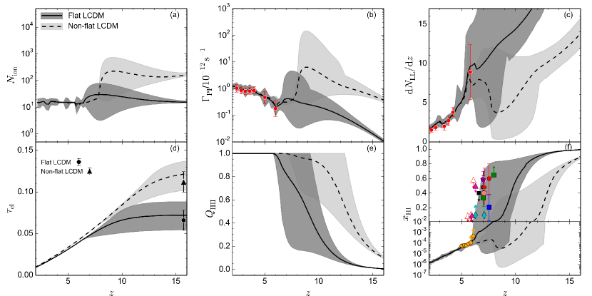
Figure 1: MCMC constraints on various quantities related to reionization obtained from the principal component analysis for tilted flat and untilted non-flat $\Lambda$CDM inflation models that best fit the Planck 2015 TT + lowP + lensing and SNIa, BAO, $H(z)$ and growth rate data (Park & Ratra, 2018a). The thick central lines along with surrounding shaded regions correspond to the best-fit models and their 2-$\sigma$ uncertainty ranges. The Panels show as a function of redshift: (a) number of ionizing photons in the IGM per baryon in stars, (b) photoionization rates for hydrogen along with observed data from Wyithe & Bolton (2011) and Becker & Bolton (2013), (c) specific number of Lyman-limit systems with the data points combined from Songaila & Cowie (2010) and Prochaska et al. (2010), (d) electron scattering optical depths along with their values from Park & Ratra (2018a), (e) volume filling factor of ionized regions, and (f) global neutral hydrogen fraction with various current observational limits. See the main text for references.

The MCMC results for the tilted flat and untilted non-flat $\Lambda$CDM inflation models are shown in Fig. 1. The thick central solid lines and dark shaded regions surrounding them correspond to the mean values and 2-$\sigma$ (95% C.L.) uncertainty ranges, respectively, of different quantities related to reionization history for the standard tilted flat $\Lambda$CDM model. On the other hand, the thick central dashed lines and light shaded regions represent the same for the untilted non-flat $\Lambda$CDM model. The MCMC constraints on all these quantities are much tighter for redshift $z\lesssim 6$, as most of the reionization-related datasets considered in our analysis exist only at these redshifts. However, evolution in the $z>6$ region essentially depends on the optical depth data ($\tau_{\rm el}$) alone, and that’s why a weaker constraint is expected in this redshift regime. The errors further decrease at $z>12$ as the components of the Fisher matrix are zero at higher redshifts due to the fact that there exist no free electrons to contribute to $\tau_{\rm el}$ at that regime, and thus forcing the mean model to converge towards the fiducial one. Also note that the evolution is almost identical for the flat and non-flat cases at $z\lesssim 6$, however, at earlier epochs their evolutionary histories differ considerably, as expected from the significantly different values of optical depths in the two models.

The evolution of $N_{\rm ion}(z)$ obtained from the MCMC statistics is shown in Panel (a). We see that an almost constant or non-evolving $N_{\rm ion}$ is sufficient to explain the reionization history in flat $\Lambda$CDM, whereas this quantity must increase at $z\gtrsim 7$ for the non-flat model. This is due to the fact that, the value of $\tau_{\rm el}$ is quite high ($\sim 0.11$) for this case, and $N_{\rm ion}$ has to evolve quite rapidly at higher redshifts to match such a value. This hints that either chemical feedback from Pop III stars and/or an evolving star-forming efficiency or photon escape fraction or both play a significant role in the non-flat $\Lambda$CDM model. We have shown the evolution of $\Gamma_{\rm PI}$ and ${\rm d}N_{\rm LL}/{\rm d}z$ in Panels (b) and (c) respectively along with their observed data (red points with error bars) that we have included in our MCMC analysis. Clear non-monotonic trends with redshift are also visible here for the non-flat case. $\Gamma_{\rm PI}$ is quite large at earlier epochs in this model compared to that for the flat one, indicating a possibility of Pop III stars being the major contributers of ionizing photons at those epochs. As expected, the $\tau_{\rm el}$, shown in Panel (d), reasonably match the current data points from the results of Park & Ratra (2018a). However, its upper limits for both the flat and non-flat models are found to be slightly higher than their observed values, suggesting that a wide range of early reionization models are still permitted by the data. Panel (e) shows the evolution of volume filling factor of ionized (HII) region, $Q_{\rm HII}(z)$ (defined as the fraction of IGM volume that is filled up by ionized regions). From this plot one can see that for the tilted flat $\Lambda$CDM model the mean growth of $Q_{\rm HII}(z)$ is quite smooth and reionization is almost completed, i.e. $Q_{\rm HII}(z)\sim 1$, around $6\lesssim z\lesssim 9$ (95% C.L.). On the other hand the untilted non-flat model shows a much faster rise at initial stages starting as early as $z\approx 14$ and then gradually approaches towards the end-stage of reionization which completes around $7\lesssim z\lesssim 12$ (95% C.L.). A more extended reionization scenario is needed for the non-flat case so that enough contribution to $\tau_{\rm el}$ is acquired in order to match the high value.

A similar conclusion can also be drawn from the evolution of the neutral hydrogen fraction $x_{\rm HI}(z)$ in Panel (f). For comparison, here we have shown various recent observational limits on this quantity. The most important constraints at the end-stage of cosmic reionization come from the Gunn-Peterson optical depth data of high-redshift ($z\approx 5-6$) quasars measured by Fan et al. (2006b) (filled yellow circles). Measurements from the near zone of bright quasars by Schroeder et al. (2013) and Bolton et al. (2011) are shown in the figure by filled cyan diamonds. Constraints on the neutral fraction from the damping wing analysis of highest redshift ($z=7.09$ and $7.54$) quasars by Greig et al. (2017) and Davies et al. (2018) are also shown here by the filled salmon circle and red hexagons respectively. Recently, a more model-independent analysis by Greig et al. (2019) on the $z=7.54$ QSO recovers a slightly lower value of $x_{\rm HI}=0.21^{+0.17}_{-0.19}$ (1-$\sigma$ error; shown by the filled blue square in the figure) than that reported in Davies et al. (2018). We show the constraints from observed GRB host galaxies at $z\sim 6.3$ (Totani et al., 2006) and $z\sim 5.9$ (Chornock et al., 2013) by filled pink triangles. Apart from quasars and GRBs, the high-redshift Lyman$\alpha$ emitters (LAEs) are also a reliable probe for the epoch of reionization. In the plot, we show them by filled black squares (Ota et al., 2008; Ouchi et al., 2010), green squares (Schenker et al., 2014), and a filled purple pentagon (Mason et al., 2018). Note that most of the observational constraints at $z\gtrsim 7$ are extremely model-dependent and might get modified in the future, that’s why we did not include those in our analysis. A more useful constraint for us comes from a model-independent analysis of high redshift ($z\sim 5.6$ and $5.9$) quasar spectra by McGreer et al. (2015) (open red triangles) which we impose in our current MCMC analysis as priors. One can see that the flat model can comfortably accommodate all these observational constraints on $x_{\rm HI}$, considering its 2-$\sigma$ region, whereas the non-flat model with larger $\tau_{\rm el}$ value struggles to match these limits. In fact, any reionization model that produces a higher optical depth results in a smaller neutral fraction at earlier times (see e.g., Robertson et al. 2013; Robertson et al. 2015; Bouwens et al. 2015; Mitra et al. 2015, 2018b). We note, however, that the Planck 2018 $\tau_{\rm el}$ value in the six parameter tilted flat $\Lambda$CDM inflation model is about 0.9-$\sigma$ lower than the corresponding $\tau_{\rm el}$ value we use here; accounting for this will alleviate some of the discrepancy between the untilted non-flat $\Lambda$CDM model predictions and the observations.

3.2 Constraints on dynamical dark energy models

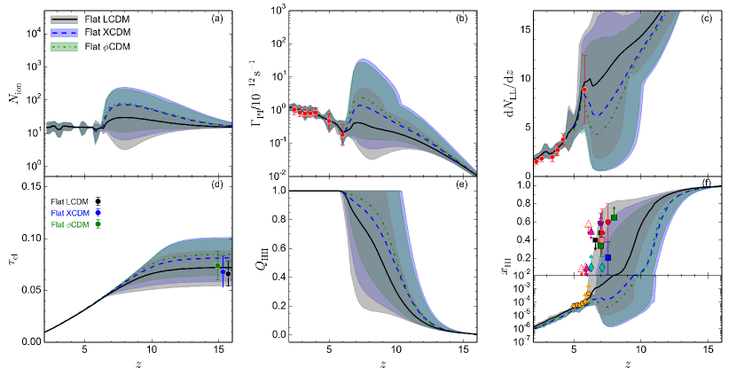
Figure 2: Same as Fig. 1, but now showing the flat $\Lambda$CDM (solid central lines with surrounding gray shaded 2-$\sigma$ regions), flat XCDM (Park & Ratra 2018a; dashed central lines with surrounding blue shaded 2-$\sigma$ regions), and flat $\phi$CDM (Park & Ratra 2018c; dot-dashed central lines with surrounding green shaded 2-$\sigma$ region) inflation models.

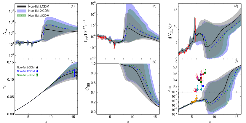
Figure 3: Same as Fig. 2, but now showing the constraints for the three non-flat inflation models.

We also perform a similar analysis for flat and non-flat XCDM and $\phi$CDM dynamical dark energy inflation models and these results are shown in Figs. 2 and 3 respectively. The evolution of all the quantities in these models have been indicated by dashed central lines with surrounding blue shaded 2-$\sigma$ regions (for XCDM) and dot-dashed central lines with surrounding green shaded 2-$\sigma$ regions (for $\phi$CDM). For comparison, the $\Lambda$CDM models are shown by solid central lines with surrounding gray shaded 2-$\sigma$ regions.

The first thing to notice is that, irrespective of the nature of dark energy, models with similar reionization optical depths behave similarly. For all the flat models with relatively lower $\tau_{\rm el}$ ($\approx 0.06$—0.07), cosmic reionization can be accomplished by a single stellar population (Pop II stars). Although the mean evolution of $N_{\rm ion}(z)$ shows a slight increase at $z\gtrsim 6$, a constant model is still permitted within its 2-$\sigma$ C.L. On the other hand, for all the non-flat models with $\tau_{\rm el}\approx 0.11-0.12$, reionization has to be driven by other stellar populations, perhaps Pop III stars, at earlier epochs. The corresponding $\tau_{\rm el}$ data are shown in Panel (d) by the colored points with error bars. As additional regions get ionized, the combined action of chemical and radiative feedback suppresses Pop III star formation and after that the Pop II stellar population dominates the reionization process at lower redshifts ($z\lesssim 8$). Such models indicate a much faster evolution of $Q_{\rm HII}(z)$ at initial stages, and then gradually approach towards the end-stage of the epoch of reionization. Unlike flat models, the non-flat ones hint at a much earlier and more extended reionization scenario that is completed around $z\approx 7$. In fact, we find that higher the optical depth, the more extended is the reionization process. Also, the neutral hydrogen fraction obtained from the non-flat models is much smaller at higher redshifts ($z>7$) compared to the flat cases, which makes these models likely to be disfavored by most current high-redshift observations from distant QSOs, GRBs and LAEs (see Panel (f) of Fig. 3). However, the Planck 2018 reduction in $\tau_{\rm el}$ in the six parameter tilted flat $\Lambda$CDM inflation model by about 0.9-$\sigma$ will somewhat help reconcile the non-flat model predictions with these observations.

3.3 Evolution of the escape fraction

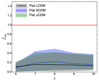
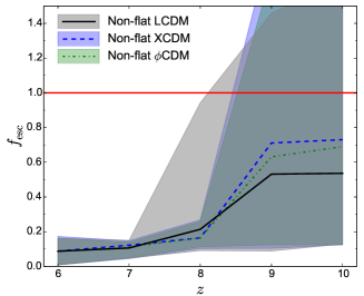
Figure 4: Redshift evolution of the escape fraction $f_{\rm esc}(z)$ along with its 2-$\sigma$ errors for all the flat (left panel) and non-flat (right panel) models considered in this work. The red solid lines in both panels correspond to an escape fraction of unity.

It is clear that all non-flat models, irrespective of the nature of dark energy, predict very high $N_{\rm ion}$ values and their strong evolution with redshift. This prompts us to check whether the escape fraction of ionizing photons from PopII stars for such models becomes unrealistically high at some redshifts. This quantity can be obtained by comparing the observed evolution of the high-$z$ galaxy UV Luminosity Function (LF) with the predictions from our reionization models. There already exist many in-depth studies for this, see e.g., Samui et al. (2007, 2009); Kulkarni & Choudhury (2011); Mitra et al. (2013, 2015). We refer the reader to those for the detailed methodology.

The basic idea is to compute the luminosity function $\Phi(M_{AB},z)$, where $M_{AB}$ is the absolute AB magnitude, from the luminosity at $1500$ $\mathring{\rm A}$ of a galaxy which in turn depends on the star-forming efficiency $\epsilon_{*}$. We then vary $\epsilon_{*}$ as a free parameter to match the observed LFs at redshifts $z=6-10$. Although not shown in the present paper, we find that a roughly constant ($\sim 4\%$; best-fit value) $\epsilon_{*}$ is needed for all the flat and non-flat models considered here (see Fig. 2 of Paper I; Mitra et al. 2018b). We can then get limits for $f_{\rm esc}$ at different redshifts from Eq. (12) using the MCMC constraints already obtained on the evolution of $N_{\rm ion}(z)$. Note that we take the value of $N_{\gamma}$ as $\approx 3200$ which is appropriate for the PopII Salpeter IMF assumed here.

The redshift evolution of $f_{\rm esc}$ for different models are shown in Fig. 4. The corresponding 2-$\sigma$ uncertainties, indicated by shaded regions in the plot, have been computed using the quadrature method (Mitra et al., 2013). We find that the best-fit $f_{\rm esc}$ remains almost constant at $\sim 10-20\%$ for the whole redshift range in all the flat models (left panel). On the other hand a strong redshift evolution of this quantity is required for the non-flat models (right panel) – it can increase by a factor of $\sim 7$ from redshift $6$ to $10$. Moreover, if we consider their 2-$\sigma$ ranges, these non-flat models can lead to an impractically high $f_{\rm esc}$ ($\gtrsim 1$) at redshifts $z\gtrsim 8$. The sole reason behind such trends is that the values of $N_{\rm ion}$ for non-flat models can become as high as $\sim 1000$ around $z\approx 8-9$, considering their 2-$\sigma$ limits (see panel (a) of Fig. 3), in order to produce very high optical depths required for those models. On the other hand, the upper limits (2-$\sigma$) of escape fraction for the flat models having relatively lower $\tau_{\rm el}$, can become at most $50\%$ for all the redshift ranges considered here. Such one-to-one correspondence between strong redshift evolution of $f_{\rm esc}(z)$ and higher reionization optical depths has also been reported earlier in many studies, see e.g., Haardt & Madau (2012); Kuhlen & Faucher-Giguère (2012); Mitra et al. (2013).

4 Concluding remarks

We have presented detailed statistical analysis of reionization in tilted flat and untilted non-flat $\Lambda$CDM, XCDM and $\phi$CDM inflation models. The cosmological parameters for these models are constrained by Planck 2015 TT + lowP + lensing CMB anisotropy and SNIa, BAO, $H(z)$, and growth rate data, using physically motivated inflation power spectra for energy density inhomogeneities (Park & Ratra, 2018a, c). For the non-flat models, these data prefer mildly closed models with $\Omega_{\rm k}\sim-0.006$ to $-0.008$. Although such models provide better fits to the observed low-$\ell$ temperature anisotropy $C_{\ell}$’s and weak-lensing $\sigma_{8}$ estimates, they provide worse fits to the observed higher-$\ell$ temperature anisotropy $C_{\ell}$’s and primordial deuterium abundances (Penton et al., 2018). These closed models also predict relatively higher reionization optical depth values ($\tau_{\rm el}\approx 0.11$—0.12) compared to those obtained from the flat ones. This could lead to a significantly different reionization scenario at higher redshifts $z>6$ in the non-flat cases. To get constraints on reionization parameters, we decompose, an unknown but yet a very crucial quantity, $N_{\rm ion}(z)$, the number of photons in the IGM per baryon, into its principal components and perform a thorough MCMC analysis on the PCA modes using joint datasets of quasars and the corresponding $\tau_{\rm el}$ for each model. Our analysis method is quite similar to that presented in Paper I (Mitra et al., 2018b).

Our main findings, in summary, are:

• We find that all six models behave very similarly in the lower redshift region ($z\lesssim 6$) and can comfortably match all available observational data here, whereas at earlier epochs they differ significantly, as expected, due to the different optical depth values of the models.

• All the non-flat models, irrespective of their nature of dark energy, demand a strong redshift evolution in $N_{\rm ion}(z)$ at $z>6$ in order to produce the higher $\tau_{\rm el}$ values. This could hint at the possibility of reionization driven by early stellar sources like Pop III stars and/or a rapidly increasing star formation efficiency and/or photon escape fraction. On the other hand, a constant $N_{\rm ion}$ is sufficient to explain reionization in flat models.

• Models with higher optical depths result in a relatively extended and early reionization completing around $7\lesssim z\lesssim 13$ (from 2-$\sigma$ limits for $Q_{\rm HII}\sim 1$). Also, such models predict a much lower neutral hydrogen fraction at higher redshifts ($z\gtrsim 7$). Such small values, e.g. $<0.2$ at $z\sim 8$, are clearly in tension with most of the current observational limits from distant Ly$\alpha$ emitters.

Another serious drawback of the non-flat models can be seen from the evolution of the photon escape fraction $f_{\rm esc}(z)$. In Fig. 4, we have shown that models with very large $N_{\rm ion}$ at higher redshifts give rise to an unrealistically high escape fraction at those redshifts. We find that $f_{\rm esc}$ in the non-flat models can become $\gtrsim 1$ even at $z\gtrsim 8$, considering its 2-$\sigma$ limits. Such unphysical values of $f_{\rm esc}$ point to the possibility of ruling out those models. On the other hand, a constant escape fraction of $\sim 10-20\%$ (best-fit) is adequate for all the flat models. Note that, we did not include the high-redshift ($z>7$) observational bounds on $x_{\rm HI}$ in our current analysis as these are quite weak and largely model-dependent in nature (Dayal et al., 2009; Bolton & Haehnelt, 2013; Choudhury et al., 2015; Kakiichi et al., 2016; Weinberger et al., 2018). But even if we incorporate such data in the model to discard some of the very early reionization scenarios which are otherwise allowed in the non-flat cases, the evolution of various reionization quantities can become significantly non-monotonic, which is quite unphysical in nature and thus should be disfavored. For detailed discussion on this, we refer the reader to our Paper I (Mitra et al., 2018b).

It is now well recognized that the high-redshift LAE data favor a late reionization (Mesinger et al., 2015; Choudhury et al., 2015) and the non-flat models having large $\tau_{\rm el}$ values clearly struggle to match these data. This raises the possibility of ruling out such models in view of those current observational limits. Unrealistic escape fractions also push the non-flat models to the verge of being ruled out. We emphasize however that the lower Planck 2018 $\tau_{\rm el}$ will alleviate some of this tension; it remains to be established whether this $\tau_{\rm el}$ reduction can alleviate all of the tension.

On the other hand, all the flat models, irrespective of the nature of dark energy, behave almost the same, making it difficult to distinguish between them by using available data. One has to rely on future observations of more high-redshift quasars, LAEs, and possible detection of the redshifted 21-cm signal from the epoch of reionization to resolve this issue, and possibly establish or rule out dark energy dynamics.

References

- Akama & Kobayashi (2019) Akama S., Kobayashi T., 2019, Phys. Rev. D, 99, 043522
- Alam et al. (2017) Alam S., et al., 2017, MNRAS, 470, 2617
- Avsajanishvili et al. (2015) Avsajanishvili O., Samushia L., Arkhipova N. A., Kahniashvili T., 2015, arXiv e-prints, p. arXiv:1511.09317
- Bailey (2012) Bailey S., 2012, Publications of the Astronomical Society of the Pacific, 124, 1015
- Barkana & Loeb (2001) Barkana R., Loeb A., 2001, Phys. Rep., 349, 125
- Becker & Bolton (2013) Becker G. D., Bolton J. S., 2013, MNRAS, 436, 1023
- Bolton & Haehnelt (2013) Bolton J. S., Haehnelt M. G., 2013, MNRAS, 429, 1695
- Bolton et al. (2011) Bolton J. S., et al., 2011, MNRAS, 416, L70
- Bouwens et al. (2015) Bouwens R. J., Illingworth G. D., Oesch P. A., Caruana J., Holwerda B., Smit R., Wilkins S., 2015, ApJ, 811, 140
- Chornock et al. (2013) Chornock R., et al., 2013, ApJ, 774, 26
- Choudhury (2009) Choudhury T. R., 2009, Current Science, 97, 841
- Choudhury & Ferrara (2005) Choudhury T. R., Ferrara A., 2005, MNRAS, 361, 577
- Choudhury & Ferrara (2006a) Choudhury T. R., Ferrara A., 2006a, arXiv e-prints, pp astro–ph/0603149
- Choudhury & Ferrara (2006b) Choudhury T. R., Ferrara A., 2006b, MNRAS, 371, L55
- Choudhury et al. (2015) Choudhury T. R., Puchwein E., Haehnelt M. G., Bolton J. S., 2015, MNRAS, 452, 261
- Clarkson & Zunckel (2010) Clarkson C., Zunckel C., 2010, Physical Review Letters, 104, 211301
- D’Aloisio et al. (2017) D’Aloisio A., Upton Sanderbeck P. R., McQuinn M., Trac H., Shapiro P. R., 2017, MNRAS, 468, 4691
- DES Collaboration (2018) DES Collaboration 2018, arXiv e-prints, p. arXiv:1810.02499
- Davies et al. (2018) Davies F. B., et al., 2018, ApJ, 864, 142
- Dayal et al. (2009) Dayal P., Ferrara A., Saro A., Salvaterra R., Borgani S., Tornatore L., 2009, MNRAS, 400, 2000
- Efstathiou & Bond (1999) Efstathiou G., Bond J. R., 1999, MNRAS, 304, 75
- Fan et al. (2006a) Fan X., Carilli C. L., Keating B., 2006a, ARA&A, 44, 415
- Fan et al. (2006b) Fan X., et al., 2006b, AJ, 132, 117
- Farooq & Ratra (2013) Farooq O., Ratra B., 2013, ApJL, 766, L7
- Farooq et al. (2013) Farooq O., Crandall S., Ratra B., 2013, Physics Letters B, 726, 72
- Farooq et al. (2015) Farooq O., Mania D., Ratra B., 2015, Ap&SS, 357, 11
- Farooq et al. (2017) Farooq O., Madiyar F. R., Crandall S., Ratra B., 2017, ApJ, 835, 26
- Ferrara & Pandolfi (2014) Ferrara A., Pandolfi S., 2014, arXiv e-prints, p. arXiv:1409.4946
- Gott (1982) Gott III J. R., 1982, Nature, 295, 304
- Greig et al. (2017) Greig B., Mesinger A., Haiman Z., Simcoe R. A., 2017, MNRAS, 466, 4239
- Greig et al. (2019) Greig B., Mesinger A., Bañados E., 2019, MNRAS, 484, 5094
- Guha Sarkar et al. (2012) Guha Sarkar T., Mitra S., Majumdar S., Choudhury T. R., 2012, MNRAS, 421, 3570
- Haardt & Madau (2012) Haardt F., Madau P., 2012, ApJ, 746, 125
- Hamilton (2001) Hamilton A. J. S., 2001, MNRAS, 322, 419
- Hassan et al. (2018) Hassan S., Davé R., Mitra S., Finlator K., Ciardi B., Santos M. G., 2018, MNRAS, 473, 227
- Hawking (1984) Hawking S. W., 1984, Nuclear Physics B, 239, 257
- Hopkins et al. (2007) Hopkins P. F., Richards G. T., Hernquist L., 2007, ApJ, 654, 731
- Hu & Holder (2003) Hu W., Holder G. P., 2003, Phys. Rev. D, 68, 023001
- Huterer & Starkman (2003) Huterer D., Starkman G., 2003, Physical Review Letters, 90, 031301
- Inoue et al. (2006) Inoue A. K., Iwata I., Deharveng J.-M., 2006, MNRAS, 371, L1
- Ishida & de Souza (2011) Ishida E. E. O., de Souza R. S., 2011, A&A, 527, A49
- Kakiichi et al. (2016) Kakiichi K., Dijkstra M., Ciardi B., Graziani L., 2016, MNRAS, 463, 4019
- Khaire et al. (2016) Khaire V., Srianand R., Choudhury T. R., Gaikwad P., 2016, MNRAS, 457, 4051
- Kuhlen & Faucher-Giguère (2012) Kuhlen M., Faucher-Giguère C.-A., 2012, MNRAS, 423, 862
- Kulkarni & Choudhury (2011) Kulkarni G., Choudhury T. R., 2011, MNRAS, 412, 2781
- Leach (2006) Leach S., 2006, MNRAS, 372, 646
- Lewis & Bridle (2002) Lewis A., Bridle S., 2002, Phys. Rev. D, 66, 103511
- Lidz (2016) Lidz A., 2016, in Mesinger A., ed., Astrophysics and Space Science Library Vol. 423, Understanding the Epoch of Cosmic Reionization: Challenges and Progress. p. 23 (arXiv:1511.01188), doi:10.1007/978-3-319-21957-8_2
- Loeb & Barkana (2001) Loeb A., Barkana R., 2001, ARA&A, 39, 19
- Lucchin & Matarrese (1985) Lucchin F., Matarrese S., 1985, Phys. Rev. D, 32, 1316
- Luković et al. (2018) Luković V. V., Haridasu B. S., Vittorio N., 2018, Foundations of Physics, 48, 1446
- Madau & Haardt (2015) Madau P., Haardt F., 2015, ApJL, 813, L8
- Madau et al. (1999) Madau P., Haardt F., Rees M. J., 1999, ApJ, 514, 648
- Mainini et al. (2003) Mainini R., Macciò A. V., Bonometto S. A., Klypin A., 2003, ApJ, 599, 24
- Martin (2012) Martin J., 2012, Comptes Rendus Physique, 13, 566
- Mason et al. (2018) Mason C. A., Treu T., Dijkstra M., Mesinger A., Trenti M., Pentericci L., de Barros S., Vanzella E., 2018, ApJ, 856, 2
- McGreer et al. (2015) McGreer I. D., Mesinger A., D’Odorico V., 2015, MNRAS, 447, 499
- Mesinger et al. (2015) Mesinger A., Aykutalp A., Vanzella E., Pentericci L., Ferrara A., Dijkstra M., 2015, MNRAS, 446, 566
- Miralda-Escudé et al. (2000) Miralda-Escudé J., Haehnelt M., Rees M. J., 2000, ApJ, 530, 1
- Miranda et al. (2015) Miranda V., Hu W., Dvorkin C., 2015, Phys. Rev. D, 91, 063514
- Mitra et al. (2011) Mitra S., Choudhury T. R., Ferrara A., 2011, MNRAS, 413, 1569
- Mitra et al. (2012) Mitra S., Choudhury T. R., Ferrara A., 2012, MNRAS, 419, 1480
- Mitra et al. (2013) Mitra S., Ferrara A., Choudhury T. R., 2013, MNRAS, 428, L1
- Mitra et al. (2015) Mitra S., Choudhury T. R., Ferrara A., 2015, MNRAS, 454, L76
- Mitra et al. (2018a) Mitra S., Choudhury T. R., Ferrara A., 2018a, MNRAS, 473, 1416
- Mitra et al. (2018b) Mitra S., Choudhury T. R., Ratra B., 2018b, MNRAS, 479, 4566
- Mohammed & Gnedin (2018) Mohammed I., Gnedin N. Y., 2018, ApJ, 863, 173
- Mortonson & Hu (2008) Mortonson M. J., Hu W., 2008, ApJ, 672, 737
- Mukherjee et al. (2019) Mukherjee A., Paul N., Jassal H. K., 2019, JCAP, 1, 005
- Natarajan & Yoshida (2014) Natarajan A., Yoshida N., 2014, Progress of Theoretical and Experimental Physics, 2014, 06B112
- Okamoto et al. (2008) Okamoto T., Gao L., Theuns T., 2008, MNRAS, 390, 920
- Ooba et al. (2018a) Ooba J., Ratra B., Sugiyama N., 2018a, arXiv e-prints, p. arXiv:1802.05571
- Ooba et al. (2018b) Ooba J., Ratra B., Sugiyama N., 2018b, ApJ, 864, 80
- Ooba et al. (2018c) Ooba J., Ratra B., Sugiyama N., 2018c, ApJ, 866, 68
- Ooba et al. (2018d) Ooba J., Ratra B., Sugiyama N., 2018d, ApJ, 869, 34
- Ota et al. (2008) Ota K., et al., 2008, ApJ, 677, 12
- Ouchi et al. (2010) Ouchi M., et al., 2010, ApJ, 723, 869
- Park & Ratra (2017) Park C.-G., Ratra B., 2017, arXiv e-prints, p. arXiv:1801.00213
- Park & Ratra (2018a) Park C.-G., Ratra B., 2018a, arXiv e-prints, p. arXiv:1803.05522
- Park & Ratra (2018b) Park C.-G., Ratra B., 2018b, arXiv e-prints, p. arXiv:1809.03598
- Park & Ratra (2018c) Park C.-G., Ratra B., 2018c, ApJ, 868, 83
- Park et al. (2019) Park J., Mesinger A., Greig B., Gillet N., 2019, MNRAS, p. 37
- Pavlov et al. (2013) Pavlov A., Westmoreland S., Saaidi K., Ratra B., 2013, Phys. Rev. D, 88, 123513
- Peebles (1984) Peebles P. J. E., 1984, ApJ, 284, 439
- Peebles & Ratra (1988) Peebles P. J. E., Ratra B., 1988, ApJL, 325, L17
- Penton et al. (2018) Penton J., Peyton J., Zahoor A., Ratra B., 2018, Publ. Astr. Soc. Pac., 130, 114001
- Planck Collaboration (2016) Planck Collaboration 2016, A&A, 594, A13
- Planck Collaboration (2018) Planck Collaboration 2018, arXiv e-prints, p. arXiv:1807.06209
- Press & Schechter (1974) Press W. H., Schechter P., 1974, ApJ, 187, 425
- Prochaska et al. (2010) Prochaska J. X., O’Meara J. M., Worseck G., 2010, ApJ, 718, 392
- Qi et al. (2019) Qi J.-Z., Cao S., Zhang S., Biesiada M., Wu Y., Zhu Z.-H., 2019, MNRAS, 483, 1104
- Ratra (1985) Ratra B., 1985, Phys. Rev. D, 31, 1931
- Ratra (1989) Ratra B., 1989, Phys. Rev. D, 40, 3939
- Ratra (1992) Ratra B., 1992, Phys. Rev. D, 45, 1913
- Ratra (2017) Ratra B., 2017, Phys. Rev. D, 96, 103534
- Ratra & Peebles (1988) Ratra B., Peebles P. J. E., 1988, Phys. Rev. D, 37, 3406
- Ratra & Peebles (1995) Ratra B., Peebles P. J. E., 1995, Phys. Rev. D, 52, 1837
- Ratra & Vogeley (2008) Ratra B., Vogeley M. S., 2008, Publ. Astr. Soc. Pac., 120, 235
- Regan & Munshi (2015) Regan D., Munshi D., 2015, MNRAS, 448, 2232
- Robertson et al. (2013) Robertson B. E., et al., 2013, ApJ, 768, 71
- Robertson et al. (2015) Robertson B. E., Ellis R. S., Furlanetto S. R., Dunlop J. S., 2015, ApJL, 802, L19
- Ryan et al. (2018) Ryan J., Doshi S., Ratra B., 2018, MNRAS, 480, 759
- Ryan et al. (2019) Ryan J., Chen Y., Ratra B., 2019, arXiv e-prints, p. arXiv:1902.03196
- Samui et al. (2007) Samui S., Srianand R., Subramanian K., 2007, MNRAS, 377, 285
- Samui et al. (2009) Samui S., Srianand R., Subramanian K., 2009, MNRAS, 398, 2061
- Samushia & Ratra (2010) Samushia L., Ratra B., 2010, ApJ, 714, 1347
- Samushia et al. (2007) Samushia L., Chen G., Ratra B., 2007, arXiv e-prints, p. arXiv:0706.1963
- Sangwan et al. (2018) Sangwan A., Tripathi A., Jassal H. K., 2018, arXiv e-prints, p. arXiv:1804.09350
- Sasaki & Suzuki (2019) Sasaki T., Suzuki H., 2019, Phys. Rev. D, 99, 063502
- Schenker et al. (2014) Schenker M. A., Ellis R. S., Konidaris N. P., Stark D. P., 2014, ApJ, 795, 20
- Schroeder et al. (2013) Schroeder J., Mesinger A., Haiman Z., 2013, MNRAS, 428, 3058
- Scolnic et al. (2018) Scolnic D. M., et al., 2018, ApJ, 859, 101
- Singh et al. (2018) Singh A., Sangwan A., Jassal H. K., 2018, arXiv e-prints, p. arXiv:1811.07513
- Sobacchi & Mesinger (2013) Sobacchi E., Mesinger A., 2013, MNRAS, 432, 3340
- Solà et al. (2017) Solà J., Gómez-Valent A., de Cruz Pérez J., 2017, Modern Physics Letters A, 32, 1750054
- Sola et al. (2018) Sola J., Gomez-Valent A., de Cruz Perez J., 2018, arXiv e-prints, p. arXiv:1811.03505
- Songaila & Cowie (2010) Songaila A., Cowie L. L., 2010, ApJ, 721, 1448
- Sumida et al. (2018) Sumida T., Kashino D., Hasegawa K., 2018, MNRAS, 475, 3870
- Tosone et al. (2019) Tosone F., Haridasu B. S., Luković V. V., Vittorio N., 2019, Phys. Rev. D, 99, 043503
- Totani et al. (2006) Totani T., et al., 2006, Pub. Astron. Soc. Japan, 58, 485
- Wang et al. (2018) Wang Y., Pogosian L., Zhao G.-B., Zucca A., 2018, ApJL, 869, L8
- Wei (2018) Wei J.-J., 2018, ApJ, 868, 29
- Weinberger et al. (2018) Weinberger L. H., Kulkarni G., Haehnelt M. G., Choudhury T. R., Puchwein E., 2018, MNRAS, 479, 2564
- Witzemann et al. (2018) Witzemann A., Bull P., Clarkson C., Santos M. G., Spinelli M., Weltman A., 2018, MNRAS, 477, L122
- Wyithe & Bolton (2011) Wyithe J. S. B., Bolton J. S., 2011, MNRAS, 412, 1926
- Xu et al. (2018) Xu H., Huang Z., Liu Z., Miao H., 2018, arXiv e-prints, p. arXiv:1812.09100
- Yang et al. (2018) Yang W., Shahalam M., Pal B., Pan S., Wang A., 2018, arXiv e-prints, p. arXiv:1810.08586
- Yashar et al. (2009) Yashar M., Bozek B., Abrahamse A., Albrecht A., Barnard M., 2009, Phys. Rev. D, 79, 103004
- Yu et al. (2018) Yu H., Ratra B., Wang F.-Y., 2018, ApJ, 856, 3
- Zaroubi (2013) Zaroubi S., 2013, in Wiklind T., Mobasher B., Bromm V., eds, Astrophysics and Space Science Library Vol. 396, The First Galaxies. p. 45 (arXiv:1206.0267), doi:10.1007/978-3-642-32362-1_2
- Zhai et al. (2017) Zhai Z., Blanton M., Slosar A., Tinker J., 2017, ApJ, 850, 183
- Zhang et al. (2017) Zhang Y.-C., Zhang H.-Y., Wang D.-D., Qi Y.-H., Wang Y.-T., Zhao G.-B., 2017, Research in Astronomy and Astrophysics, 17, 050
- Zhang et al. (2019) Zhang J.-J., Lee C.-C., Geng C.-Q., 2019, Chinese Physics C, 43, 025102
- Zheng et al. (2019) Zheng J., Melia F., Zhang T.-J., 2019, arXiv e-prints, p. arXiv:1901.05705