Testing the Impact of Satellite Anisotropy on Large and Small Scale Intrinsic Alignments using Hydrodynamical Simulations

Abstract

Galaxy intrinsic alignments (IAs) have long been recognised as a significant contaminant to weak lensing-based cosmological inference. In this paper we seek to quantify the impact of a common modelling assumption in analytic descriptions of intrinsic alignments: that of spherically symmetric dark matter halos. Understanding such effects is important as the current generation of intrinsic alignment models are known to be limited, particularly on small scales, and building an accurate theoretical description will be essential for fully exploiting the information in future lensing data. Our analysis is based on a catalogue of 113,560 galaxies between $z=0.06-1.00$ from MassiveBlack-II, a hydrodynamical simulation of box length $100h^{-1}$ Mpc. We find satellite anisotropy contributes at the level of $\geq 30-40\%$ to the small scale alignment correlation functions. At separations larger than $1h^{-1}$ Mpc the impact is roughly scale-independent, inducing a shift in the amplitude of the IA power spectra of $\sim 20\%$. These conclusions are consistent across the redshift range and between the MassiveBlack-II and illustris simulations. The cosmological implications of these results are tested using a simulated likelihood analysis. Synthetic cosmic shear data is constructed with the expected characteristics (depth, area and number density) of a future LSST-like survey. Our results suggest that modelling alignments using a halo model based upon spherical symmetry could potentially induce cosmological parameter biases at the $\sim 1.5\sigma$ level for $S_{8}$ and $w$.

1 Introduction

In many ways the field of cosmology has changed irrevocably in the past decade. With large-volume measurements from a new generation of instruments, it has finally become possible to test the predictions of theorists to meaningful precision. So much is this the case that the distinction between “theorist” and “observer” has increasingly less meaning; cutting edge cosmology is now a process of using ever more powerful datasets to constrain, test, break and ultimately rebuild our models of the Universe. This is particularly true of weak lensing cosmology, which began to flourish somewhat later than the study of the Cosmic Microwave Background (CMB) as a cosmological probe. The transition into a data-led high-precision discipline has, by necessity, seen an increased amount of time devoted to understanding the numerous, often subtle, sources of systematic error. Without such efforts, as a community, our ability to constrain the cosmological parameters encoded in large scale structure will very quickly become limited by systematics. For an overview of recent developments in lensing cosmology we refer the reader to contemporary reviews on the subject (Kilbinger, 2015; Mandelbaum, 2018).

Often new methods have been developed to circumvent limitations in our ability to deal with certain systematics. One good example is the case of shear measurement bias, which is inherent to the process of inferring galaxy ellipticities. A coherent community effort (Heymans et al., 2006; Massey et al., 2007; Bridle et al., 2010; Kitching et al., 2011; Mandelbaum et al., 2015) has seen the development of several novel techniques, which can calibrate shear biases to sub-percentage level without the need for massive high-fidelity image simulations (Bernstein et al., 2016; Huff & Mandelbaum, 2017; Sheldon & Huff, 2017). There are hopes that a combination of innovations such as multi-object fitting (Drlica-Wagner et al., 2018), internal self-calibration (see Dark Energy Survey Collaboration 2017; Joudaki et al. 2018 for practical implementations) and improved spectroscopic overlap will bring similar advances in the case of photometric redshift (photo-$z$) error.

Amongst various other lensing systematics, a phenomenon known as intrinsic alignments (IAs) poses significant theoretical challenges for future analyses. Generally, the term “intrinsic alignments” covers two slightly different physical effects; physically close pairs of galaxies will tend to align with each other through interaction with local large scale structure, producing weak positive alignment (known as II correlations; Catelan et al. 2001; Crittenden et al. 2001). Often the dominant form of IA contamination, however, comes in the form of GI correlations (Hirata & Seljak, 2004). These arise due to the fact that mass on the line of sight simultaneously lenses background objects and tidally interacts with nearby galaxies. There are a good many reviews on the subject of intrinsic alignment in the literature, to which we refer the reader for more details (Troxel & Ishak, 2015; Joachimi et al., 2015; Kirk et al., 2015; Kiessling et al., 2015).

Unlike many potential sources of bias, IAs are inherently astrophysical in nature, rather than the result of flaws in the measurement process. No amount of ingenuity will alter the fact that such correlations are present in the data and enter on similar angular scales to cosmic shear. That neglecting intrinsic alignments when modelling cosmic shear or galaxy-galaxy lensing will induce significant $(\gg 1\sigma)$ biases in one’s recovered cosmological parameters is now well established (Krause et al., 2016; Blazek et al., 2017). In practice the most feasible way of mitigating intrinsic alignments is to simply model them out, including additional parameters in any likelihood analysis, which are marginalised over with wide priors. Unfortunately the efficacy of such a technique is somewhat limited by the models in question; to marginalise out the impact of IAs without residual biases, one requires a sufficiently accurate model to describe their impact. Due to limitations in both theory and available data, however, no model has been demonstrated to be accurate for all galaxy types at the level needed for future surveys. Understanding intrinsic alignments at the level of basic physical phenomenology, and from a theoretical perspective is, then, crucial if the community wishes to fully exploit the cosmological information in the large-volume lensing data that will shortly become available.

The most commonly used IA model, known as the Linear Alignment Model (Hirata & Seljak, 2004) and its empirically motivated variant, the Nonlinear Alignment (NLA) Model (Bridle & King, 2007) treat intrinsic shape correlations as linear in the background tidal field. This model is well tested in the regime of low redshift luminous red galaxies (Joachimi et al., 2011; Singh et al., 2015), but observational validation is somewhat lacking in the mixed-colour samples, extending to higher redshifts, common in lensing cosmology. One approach to this problem has been to develop self-consistent perturbative models, which include both linear (tidal alignment) and quadratic (tidal torque) contributions. A small handful of such models have been published (Blazek et al., 2015; Tugendhat & Schäfer, 2018; Blazek et al., 2017) and implemented in practice (Dark Energy Survey Collaboration, 2016; Troxel et al., 2018a). An alternative approach is to build an analytic prescription for the intrinsic alignment signal using a halo model or similar. Given the known limitations of perturbation theory on the smallest scales, in the fully one-halo regime, such models are especially attractive from a theoretical perspective. Similar techniques have been employed with some success to model nonlinear growth and baryonic effects (Fedeli 2014; Schneider & Teyssier 2015; Mead et al. 2015; Mead et al. 2016) and galaxy bias (Peacock & Smith, 2000; Schulz & White, 2006; Dvornik et al., 2018). The literature around application of such methods to IAs is, however, less extensive. An early example is presented by Smith & Watts (2005), who propose a halo model based approach to modelling the alignment of triaxial dark matter halos. This was followed several years later by Schneider & Bridle (2010), wherein a similar method was developed to describe the power spectra of galaxy intrinsic alignment. Under their model galaxies are split into “centrals” and “satellites”, with the latter aligning radially towards the former within spherical halos. Such a picture is reasonably well motivated, both by theory and observational evidence (Rood & Sastry, 1972; Faltenbacher et al., 2007; Pereira et al., 2008; Sifón et al., 2015; Huang et al., 2018).

Use of such models to make analytic predictions, however, requires a number of assumptions. Generally one must assume the distribution of satellite galaxies within dark matter halos to be spherically symmetric. This is despite extensive observational and numerical evidence suggesting otherwise (see, for example, West & Blakeslee 2000, Knebe et al. 2004, Bailin et al. 2008, Agustsson & Brainerd 2010, Piscionere et al. 2015, Libeskind et al. 2016, Butsky et al. 2016, Welker et al. 2017. More discussion of the physical mechanisms that generate anisotropy and further references can be found in Zentner et al. 2005). This paper seeks to test this approximation using hydrodynamical simulations, with the aim of building a physical understanding that can be propagated into future modelling efforts; the question has attracted some level of speculation in the past, but has not hitherto been tested robustly.

This paper is structured as follows. In Section 2 we describe a set of hydrodynamical simulations used in this analysis. These datasets are public and well documented and so we will focus here on the relevant details and changes introduced for this work. A brief discussion of the sample selection used to construct our galaxy catalogues is also presented. The process for building two- and three dimensional galaxy shape information and a symmetrisation procedure, which is central to this work, are set out in Section 3. The latter part of this section then sets out a series of measurements designed to capture the impact of halo anisotropy on two-point alignment statistics, and ultimately on cosmic shear. In Section 4 we present our results, alongside a series of robustness tests intended to test the applicability of our findings. In Section 5 we present a simulated likelihood analysis with the aim of assessing the cosmological implications of modelling errors of the sort discussed in the previous sections of the paper. Section 6 concludes and offers a brief discussion of our findings.

2 A Simulacrum Universe

In this section we describe the mock universe realisations used in this work and the measurement pipeline applied to it. For a fuller description of the simulations see Khandai et al. (2015) and Vogelsberger et al. (2014). The basic statistics of the two simulations are summarised in Table 1. The pipeline from SubFind data to symmetrised galaxy catalogues and correlation functions is hosted on a public repository. The processed catalogues themselves are also available for download from https://git.io/iamod_mbiicats.

2.1 MassiveBlack-II

MassiveBlack-II is a hydrodynamical simulation in a cosmological volume of comoving dimension $L=100h^{-1}$ Mpc. The mock universe’s initial conditions were generated with a transfer function generated by CMBFAST at redshift $159$. The simulation was then allowed to evolve through to $z=0$. The basic gravitational evolution of mass is governed by the Newtonian equations of motion and the simulation run assumes a flat $\Lambda$CDM cosmology with, $\sigma_{8}=0.816$, $\Omega_{\mathrm{m}}=0.275$, $n_{\mathrm{s}}=0.968$, $\Omega_{\mathrm{b}}=0.046$, $\Omega_{\mathrm{de}}=0.725$, $h=0.701$ and $w=-1.0$.

The simulation volume contains a total of $2\times 1792^{3}$ particles (dark matter and gas); particles of dark matter and gas have mass $1.1\times 10^{7}$ and $2.2\times 10^{6}$ $h^{-1}M_{\odot}$ respectively. The simulation is based on a version of GADGET (P-GADGET; see Khandai et al. 2015; Di Matteo et al. 2012), which evaluates the gravitational forces between particles using a hierarchical tree algorithm, and represents fluids by means of smoothed particle hydrodynamics (SPH).

Star formation is governed by a Schmidt-Kennicutt law of the form $\dot{\rho}_{*}=\epsilon_{*}\rho/t_{\mathrm{ff}}$, where the left-hand term is the star formation rate density, $\rho$ is the mass density of gas and $\epsilon_{*}$ is an efficiency constant with fixed value 0.02 (Kennicutt, 1998). The denominator $t_{\mathrm{ff}}$ has units of time and corresponds to the free fall time of the gas. Star particles are generated from gas particles randomly with a probability determined by the star formation rate. The simulation run includes basic models for AGN and supernova feedback. The code models black holes as collisionless particles, which acquire mass by accreting ambient gas. As gas accretes it releases energy as photons at a rate proportional to the rate of mass growth of the black hole; the efficiency constant $\epsilon_{r}$ is assumed to have a fixed value of 0.1 (Di Matteo et al., 2012). A fixed fraction ($5\%$) of this energy is then assumed to couple with nearby gas within the softening length ($1.85$ kpc). This somewhat crude model, at least at some level, captures the influence of black hole feedback on the motion and thermodynamic state of surrounding matter. Additionally, the simulation contains a basic model for supernova feedback. Thermal instabilities in the interstellar medium are assumed to operate only above some critical density $\rho_{\mathrm{th}}$, which produces two phases of baryonic matter: clouds of cold gas surrounded by tenuous baryons at pressure equilibrium. Star formation occurs in the dense part, upon which short lifetime massive stars begin to expire, form supernovae and release fixed bursts of energy to their immediate surroundings. Conceptually similar to the black hole feedback model, this has the effect of providing localised groups of particles periodically with instantaneous boosts in energy and momentum.

2.2 illustris

To test the robustness of our results we will also incorporate public data from a second hydrodynamic simulation. Though the format of the output is ultimately the same, illustris was generated by an independent group with a number of notable methodological differences from MassiveBlack-II. We use the Illustris-1 dataset here, which was generated at a similar but non-identical $\Lambda$CDM cosmology, defined by $\sigma_{8}=0.809$, $\Omega_{\mathrm{m}}=0.2726$, $n_{\mathrm{s}}=0.963$, $\Omega_{\mathrm{b}}=0.046$, $\Omega_{\mathrm{de}}=0.7274$, $h=0.704$, $w=-1.0$.

	MassiveBlack-II	Illustris-1
Comoving Volume / $h^{-3}$ Mpc3	$100^{3}$	$75^{3}$
Particle Mass / $\times 10^{6}h^{-1}M_{\odot}$	$11.0,2.2$	$6.3,1.3$
Resolution / $h^{-1}$ Mpc	0.04	0.03

Table 1: Summary statistics for the two hydrodynamic simulations considered in the paper. The row labelled ‘particle mass’ shows dark matter, then stellar mass in units of $\times 10^{6}h^{-1}M_{\odot}$.

The data are well documented on the data release website and attendant papers (Vogelsberger et al., 2014). The simulation code makes use of an approximate model for galaxy formation, which includes gas cooling (primordial and metal line), stochastic star formation, stellar evolution, kinetic stellar feedback driven by supernovae, and supermassive black hole seeding, accretion and merging, in addition to a multi-modal model for AGN feedback. A number of tunable parameters are included in the model and the process used to decide their values is outlined by Vogelsberger et al. (2013).

2.3 Galaxy Catalogues

The following paragraphs describe the steps used to construct processed object catalogues, upon which two-point measurements are made. The discussion is largely generic to MassiveBlack-II and Illustris-1. The few points of difference between the pipeline run on the two simulations are stated explicitly.

2.3.1 Halos & Subhalos

For the purposes of this work we treat the term “galaxy” as a synonym for “subhalo with a stellar component of nonzero mass”. Particles are grouped together into halos using a friends-of-friends (FoF) algorithm, which uses an adaptive linking length of 0.2 times the mean interparticle separation. Subhalos are identified using SubFind (Springel et al., 2001). The algorithm works as follows: the local density is first calculated at the positions of all particles in a given FoF group, with a local smoothing scale set to encircle a fixed number (twenty in our case) of neighbours. The density is estimated by kernel interpolation over these neighbours. If a particle is isolated then it forms a new density peak. If it has denser neighbours in multiple different structures, an isodensity contour that crosses the saddle point is identified. In such cases the two structures are merged and flagged as a candidate subhalo if they have above some threshold number of particles.

Baseline cuts are applied to the MassiveBlack-II subhalo catalogues to remove objects with fewer than 300 star particles or 1000 dark matter particles (equivalent to mass cuts at $6.6\times 10^{8}h^{-1}M_{\odot}$ and $1.1\times 10^{10}h^{-1}M_{\odot}$ respectively). Cuts on properties such as mass will likely induce some level of selection bias in the various properties with which they correlate. They are, however, necessary to ensure subhalo convergence (see e.g. Appendix B of Chisari et al. 2018b and Section 2.3 of Tenneti et al. 2015b). This is analogous to basic level cuts on flux and likelihood in shear studies on real data; if it is not possible to derive reliable shapes (on the ensemble level) from a significant part of the galaxy sample, then one’s ability to draw physically meaningful conclusions is limited. Illustris-1 differs slightly from MassiveBlack-II in both box size and particle mass resolution, and so we adjust the cuts accordingly to maintain mass thresholds at approximately the same level. Unless explicitly stated, all results presented in this paper assume these cuts. The Illustris-1 dataset used here is smaller than MassiveBlack-II, both in raw number of galaxies surviving cuts (35,349 compared with 113,560) and in comoving number density (0.08 against 0.11 $h^{3}$ Mpc^-3). Some basic physical characteristics of the two simulations are set out in Table 1.

Redshift	No. of Galaxies	Satellite Frac.	$\sigma_{\mathrm{e}}$ (stars)	$\sigma_{\mathrm{e}}$ (matter)
0.062	0.114 M	0.351	0.411	0.354
0.300	0.121 M	0.359	0.401	0.341
0.625	0.129 M	0.366	0.390	0.330
1.000	0.136 M	0.380	0.382	0.320

Table 2: The essential characteristics of the simulated MassiveBlack-II galaxy catalogues used in this study, after baseline mass cuts. The rows represent different simulation snapshots (labelled, from top, 85, 79, 73 and 68 in the nomenclature of the data release). The satellite fraction is computed using a hybrid central definition (the most massive galaxy within the centre-most 10% of the halo radius $R$, as defined for a particular halo), which is designed to be robust to noise in the physical subhalo properties. The final two columns show the mean per-component ellipticity dispersion (i.e. $[\sigma_{e1}+\sigma_{e2}]/2$) for the projected (2D) shapes of the stellar and dark matter components of the galaxies at each redshift.

2.3.2 Central Flagging

The processed catalogues contain three binary flags for “central” galaxies, which we describe in the following paragraph. Though classifying real galaxies as centrals or satellites is common in practice, the quantities used to do so are, of course, observed ones. We do not have exact analogues in the simulations for properties such as flux and apparent magnitude. Rather, we have access to fundamentally unobservable ones such as dark matter mass and three-dimensional comoving position. Given this, we propose two alternative criteria for identifying a halo’s central galaxy: (a) the galaxy with the shortest physical distance (Euclidean separation in three dimensional comoving coordinates) from the minimum of the dark matter halo’s gravitational potential well and (b) the galaxy with the highest total mass (dark matter and stars) in the halo. We compute central flags for our catalogues using both of these definitions.

Unfortunately, each has its own limitations. Definition (a) is a split based on a significantly noisy quantity. Given the relatively fine mass resolution, it is not uncommon that what might naturally be described as a halo’s central galaxy (a large, high mass object close to the potential minimum) shares the inner region with a large number of low mass objects. The potential for misclassification is obvious; indeed we find that adopting (a) hinders our ability to reproduce observable trends (e.g. a gradual decline in satellite fraction with stellar mass) due to mislabelling of high mass central objects as satellites. Criterion (b) has similar drawbacks as a split metric. There is observational evidence (e.g. Johnston et al. 2007; Rykoff et al. 2016; Simet et al. 2017) that in many cases a halo’s most massive galaxy can be significantly offset from its centroid (as defined by the gravitational potential). By visual inspection of a subset of MassiveBlack-II halos, it is clear that such an offset is not uncommon, particularly in those undergoing mergers or with otherwise distorted, non-spherical mass distributions. We thus construct a third definition (c), under which a halo’s central is the most massive galaxy within a radius of $0.1R$ from the potential minimum, where $R=\left(GM/10^{6}h^{2}\right)^{\frac{1}{3}}$ is dependent on the total FoF halo mass $M$ and (mildly) the background cosmology. We consider (c) to be the most physically meaningful of these alternatives, and so adopt it as our fiducial definition in for the following sections. In Section 4.2 we test the robustness of our results to this analysis choice and find no qualitative change due to switching between definitions (c) and (a). Note that the flagging is performed prior to mass cuts, and so while every halo has a central galaxy under all three of these definitions, it is non-trivial that it survives in the final catalogue. The final satellite fractions in the four redshift slices used in this work are shown in Table 2. Note that (a) and (b) produce comparable values, with a similar mild increase towards high redshift. It is noticeable that the satellite fraction, defined as the total fraction of all subhalos that are not flagged as centrals, is significantly lower than 0.5, and observation that is true under all three central definitions. Though counterintuitive given the simple picture of halos with one central and a host of satellites, the catalogues contain a large number of low-mass halos with one (or fewer) subhalos. Such halos often contain no satellites and so act to dilute the global satellite fraction.

The same code pipeline is applied equivalently to SubFind outputs on both MassiveBlack-II and Illustris-1 to generate catalogues in a common format. For the galaxy catalogues used in this work and example scripts to illustrate their basic usage, see https://github.com/McWilliamsCenter/ia_modelling_public.

3 Measurements

In addition to the basic level object detection and flagging described in the previous section, a series of additional measurements are required before we can attempt to draw conclusions from the simulated data. In this section we describe the process of shape measurement, converting a collection of three dimensional particle positions associated with each subhalo into projected galaxy shapes. We then define a series of two-point statistics, on which we rely in the following sections of this paper.

3.1 Inertia Tensors & Shapes

For any practical application of weak lensing, the salient properties of a population of galaxies are its shape statistics. In real two-dimensional pixel data, one typically works with ellipticities, which may be expressed in terms of two-dimensional moments. An analogous calculation may be performed with the three-dimensional simulated galaxies in MassiveBlack-II. This is well-trodden ground, and so we will sketch out the calculation briefly and refer the readers to a host of other papers for more detail (Chisari et al., 2015; Velliscig et al., 2015; Chisari et al., 2017). A detailed presentation of alignment angles, shapes, and two-point correlations and how they depend on the chosen definition of the inertia tensor can also be found in Tenneti et al. (2015a) and Tenneti et al. (2015b). Starting from a collection of stellar or dark matter particles associated with a subhalo, we calculate the inertia tensor,

$$I_{ij}=\frac{1}{W}\sum_{\alpha=1}^{N_{\mathrm{p}}}w_{\alpha}x_{i,\alpha}x_{j,\alpha},$$ (1)

where the Roman indices indicate one of the three spatial coordinate axes $i,j\in(x,y,z)$ and the sum runs over the $N_{\mathrm{p}}$ particles within the subhalo. The positions $x_{k}$ are defined relative to the centroid of the subhalo. The coefficients $w_{\alpha}$ are particle weights and the prefactor term is the sum over weights $W=\sum_{\alpha}w_{\alpha}$. In the simplest case, which we refer to as the basic inertia tensor, particles are weighted equally and the sum of the (normalised) weights is simply the number of particles in the subhalo. This will be our default option; unless stated otherwise the reader should assume the results presented later in this paper use this definition of the inertia tensor. An alternative approach, which defines the “reduced” inertia tensor, is to weight by the inverse square of the radial distance from the subhalo centroid, $w_{\alpha}=r_{\alpha}^{-2}$. This estimator by construction downweights light on the edges of the galaxy profiles and in this sense produces projected ellipticities more akin to what might be measured from real data. It is also true, however, that imposing circularly symmetric weighting induces a bias towards low ellipticities; obtaining accurate measurements via this estimator requires an explicit correction such as the iterative method of Allgood et al. (2006).

Evaluating each element of the $3\times 3$ inertia tensor $\mathbf{I}$ provides a simple numerical description of the three-dimensional shape of the galaxy. We then decompose $\mathbf{I}$ into eigenvectors, which represent unit vectors defining the orientation of the major, intermediate and minor axes of the ellipsoid $\mathbf{A}_{\mu}=(A_{x,\mu},A_{y,\mu},A_{z,\mu})$, $\mu\in(1,2,3)$; and three eigenvalues $\lambda_{i}$, which quantify its axis lengths.

In order to fully capture higher order effects present in real data, ray-tracing and light cones would be required to generate projected per-galaxy images (see e.g. Peterson et al. 2015). Given the size of the dataset and the scope of this study, however, a simple projection along the $z$ axis of the simulation box is sufficient. Points on the projected ellipse $\mathbf{x}$ must satisfy the equation $\mathbf{x}^{\intercal}\mathbf{Q}\mathbf{x}=1$ with

$$\mathbf{Q}^{-1}=\sum_{\mu=1}^{3}\frac{\mathbf{A}_{\perp,\mu}\mathbf{A}^{\intercal}_{\perp,\mu}}{\lambda^{2}_{\mu}}-\frac{\boldsymbol{\kappa}\boldsymbol{\kappa}^{\intercal}}{\alpha^{2}},$$ (2)

and $\mathbf{A}_{\perp,\mu}=(A_{x,\mu},A_{y,\mu})$. In the above we define

$$\alpha^{2}=\sum_{\mu=1}^{3}\left(\frac{A_{z,\mu}}{\lambda_{\mu}}\right)^{2}$$ (3)

and

$$\boldsymbol{\kappa}=\sum_{\mu=1}^{3}\frac{A_{z,\mu}\mathbf{A}_{\perp,\mu}}{\lambda^{2}_{\mu}}.$$ (4)

The moments of the two dimensional ellipse $\mathbf{Q}$ can then be converted into the two ellipticity components standard in lensing via

$$(e_{1},e_{2})=\frac{(Q_{xx}-Q_{yy},2Q_{xy})}{Q_{xx}+Q_{yy}+2\sqrt{|\mathbf{Q}|}}.$$ (5)

The above recipe mirrors similar calculations in Piras et al. (2018) and Joachimi et al. (2013), to which we refer the reader for more detail. Note that we have chosen a particular ellipticity definition $e=(a-b)/(a+b)$ here. Although these quantities can be measured equivalently using dark and visible matter constituents, unless stated otherwise the results in the following sections use the latter only. This is expected to give results more directly relevant to real lensing surveys, but the impact of this decision is tested in Section 4.2.3.

3.2 Symmetrising the Distribution of Satellites in Halos

The most basic picture of the Universe sees all mass contained by discrete dark matter halos. Each of these halos then hosts a number of subhalos, some of which contain luminous matter and are thus considered detectable galaxies. In the various permutations of the halo model used in the literature, typically one assumes spherical dark matter halos and, by implication, isotropic satellite distributions about the halo centres. There is a significant amount of evidence from N-body (dark matter) simulations, however, that halos are more often than not triaxial (Kasun & Evrard, 2005; Bailin & Steinmetz, 2005; Allgood et al., 2006) and the ensemble of subhalos within them has some preferred axis (West & Blakeslee, 2000; Knebe et al., 2004; Zentner et al., 2005; Bailin et al., 2008). This implies that satellite galaxies should be similarly anisotropically distributed about the centre of their host halo, a conclusion bourne out by the limited amount of data from hydrodynamical simulations currently available.

To test the impact of this anisotropy we create an artificially symmetrised version of the galaxy catalogues described in Section 2.3. The symmetrisation process entails identifying all satellites associated with a particular halo and applying a random rotation about the halo centroid. At any particular distance from the centroid this effectively redistributes the satellites across a spherical shell of the same radius. We explicitly rotate the galaxy shapes in three dimensions, such that their relative orientation to the halo centre is preserved. Without this second rotation (position, then shape) interpretation of the physical effects at work is difficult, as the process washes out both the impact of halo asphericity and the (symmetric) gravitational influence of the host halo on galaxy shape. A cartoon diagram of this istotropisation process is shown in Figure 1.

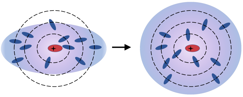
Figure 1: Two-dimensional schematic diagram of the halo symmetrisation process described in Section 3.2. The background colour gradient is intended to represent the distribution of dark matter in the halo, but is not a quantitative mapping of the halo mass profile. Galaxies (subhalos with stellar particles) are shown as filled ellipses, and the halo centroid is shown as a black cross. The black dashed lines show three isopleths of constant radius about the centroid. The central galaxy (shown in red) is unaffected, while satellites (blue ellipses) at each radius are redistributed randomly about the circle. The relative orientations of the galaxies to the centroid are explicitly maintained by the rotation.

Though conceptually very simple, the mathematics of such a three-dimensional rotation bears some thought. The aim is to transform the spherical coordinates of each satellite galaxy relative to the halo centroid as:

$$R\rightarrow R,\;\;\;\theta\rightarrow\theta^{\prime},\;\;\;\phi\rightarrow\phi^{\prime}.$$ (6)

The galaxy shape also requires an equivalent transformation in order to maintain the relative orientation to the halo centre. As implemented for this analysis the symmetrisation process involves the following steps:

• Starting from the inertia tensor of star particles in a particular satellite galaxy, we compute a $3\times 3$ eigenvector matrix $\mathbf{A}=(\mathbf{a},\mathbf{b},\mathbf{c})$, and a set of three eigenvalues $\boldsymbol{\lambda}=(\lambda_{1},\lambda_{2},\lambda_{3})$.

• Random position angles $\mathrm{cos}\theta^{\prime},\phi^{\prime}$ are drawn from uniform distributions over the range $[-1/2,1/2]$ and $[-\pi,\pi]$ respectively.

• A rotation matrix is constructed describing the transformation between the initial and the new positions, such that $\mathbf{r}^{\prime}=\mathbf{R}_{\theta}.\mathbf{r}$. The calculation of $\mathbf{R}_{\theta}$ is described in Appendix B.

• The same transformation described by the rotation matrix $\mathbf{R}_{\theta}$ is applied to each of the three orientation vectors $\mathbf{a},\mathbf{b},\mathbf{c}$, a process which preserves the relative orientation of the galaxy to its new radial position vector $\mathbf{r}^{\prime}=(R,\theta^{\prime},\phi^{\prime})$.

This leaves us with, for each satellite galaxy in a particular halo, a new rotated position $\mathbf{r}^{\prime}$ and an orientation (eigenvector) matrix $\mathbf{A}^{\prime}$. The three dimensional axis lengths $\lambda_{i}$ are unchanged by the transformation.

The symmetrisation process is designed such that it respects the periodic boundary conditions of the simulation volume. That is, galaxies in halos that traverse the box edge are shifted before rotation to form a contiguous group. In cases where rotation leaves a galaxy that was within the box outside its edges, it is shifted back to the opposite side of the volume.

3.3 Two-Point Correlation Functions

In the following we describe a series of two-point statistics used as estimators for the IA contamination to cosmic shear. All correlation functions used in this study were computed using the public halotools package (Hearin et al., 2017). The most straightforward (and highest signal-to-noise) two-point measurement one could make is that of galaxy clustering in three dimensions. We adopt a common estimator of the form (Landy & Szalay, 1993):

$$\xi_{gg}(r)=\frac{DD-2DR+RR}{RR},$$ (7)

where $DD$, $RR$ and $DR$ are counts of galaxy-galaxy, random-random and galaxy-random pairs within a physical separation bin centred on $r$. For this calculation we use 20 logarithmically spaced bins in the range $r=0.1-L/3h^{-1}$ Mpc, where $L$ is the simulation box size (100 and 75 for MassiveBlack-II and Illustris-1 respectively). For the purposes of validation, where possible, we compared our results against analogous measurements performed using TreeCorr (Jarvis et al., 2004). For galaxy-galaxy correlations we find sub-percentage level agreement between the two codes on all scales (ranging from $\sim 0.01\%$ on the smallest scales to $\sim 0.4\%$ in the two-halo regime with the default accuracy setting (bin$\_$slop=0.1); the discrepancy is seen to vanish when the computational approximations of TreeCorr are deactivated.

When considering the impact of alignments on cosmological observables ($\xi_{\pm},\gamma_{t}$ and the like), it is natural to consider two-point functions of intrinsic alignment. Beyond this broad statement, however, it is not trivial which measurement is optimal for our interests. We start by considering the most conceptually simple statistics, or the three dimensional orientation correlations. We can define two such terms,

$$\mathrm{EE}=\left<|\hat{\mathbf{e}}(\mathbf{x})\cdot\hat{\mathbf{e}}(\mathbf{x}+\mathbf{r})|^{2}\right>-\frac{1}{3}$$ (8)

where $\hat{e}$ is a unit eigenvector obtained from the inertia tensor, pointing along the major axis of the galaxy ellipsoid, and the angle brackets indicate averaging over galaxy pairs. Intuitively very simple, a positive EE correlation denotes a tendency for the major axes of galaxies to align with those of other physically close-by objects in comoving three dimensional space. Similarly:

$$\mathrm{ED}=\left<|\hat{\mathbf{e}}(\mathbf{x})\cdot\hat{\mathbf{r}}|^{2}\right>-\frac{1}{3}.$$ (9)

Here $\hat{\mathbf{r}}$ is the unit vector pointing from one galaxy to the other. In the case of ED positive values indicate radial shearing (that is, a tendency for the major axis of a galaxy to align with the direction of a neighbouring galaxy).

Though three dimensional correlations are illustrative for elucidating the mechanisms at play in the simulation they carry a number of obvious problems. Not least, they are “unobservable” in any real sense. Typically lensing studies rely on broad photometric filters and thus do not have a detailed reconstruction of where galaxies lie along the line of sight. Even with such information, reconstructing the shape of a galaxy in three dimensions is difficult-to-impossible.

We now consider “projected” correlation functions, as a closer analogue to real observable quantities. We do not, however, have access to lightcones and ray-tracing information for the MassiveBlack-II simulations. In the absence of the tools for a more sophisticated approach, we obtain real-space two dimensional statistics, rather, by projecting along the length of the simulation box.

We define the correlation function of galaxy positions and ellipticities, $\xi_{g+}(r_{\mathrm{p}},\Pi)$ as a function of 2D perpendicular separation $r_{\mathrm{p}}$ and separation along the line of sight $\Pi$. This statistic is constructed using a modified Landy-Szalay estimator of the form:

$$\xi_{g+}(r_{\mathrm{p}},\Pi)=\frac{S_{+}D-S_{+}R}{RR}$$ (10)

(see Mandelbaum et al. 2011). By analogy one can construct a shape-shape correlation function,

$$\xi_{++}(r_{\mathrm{p}},\Pi)=\frac{S_{+}S_{+}}{RR}.$$ (11)

In both cases above, $R$ represents the positions of a set of randomised positions thrown down within the simulation volume. The terms in the numerator represent shape correlations and are defined as

$$S_{+}D\equiv\frac{1}{2}\sum_{i\neq j}e_{+}(j|i),\;\;\;\;\;S_{+}S_{+}\equiv\frac{1}{4}\sum_{i\neq j}e_{+}(i|j)e_{+}(j|i),$$ (12)

where the indices $i,j$ run over galaxies and $e_{+}(j|i)$ is the tangential ellipticity of galaxy $j$, rotated into the coordinate system defined by the separation vector with galaxy $i$. With these three dimensional correlations in hand, obtaining the two dimensional versions is simply a case of integrating along the line of sight. One has,

$$w_{g+}(r_{\mathrm{p}})=\int_{-\Pi_{\mathrm{max}}}^{\Pi_{\mathrm{max}}}\mathrm{d}\Pi\xi_{g+}(r_{\mathrm{p}},\Pi)$$ (13)

and analogously

$$w_{++}(r_{\mathrm{p}})=\int_{-\Pi_{\mathrm{max}}}^{\Pi_{\mathrm{max}}}\mathrm{d}\Pi\xi_{++}(r_{\mathrm{p}},\Pi)$$ (14)

Here $\Pi_{\mathrm{max}}$ is an integration limit, which is set by the simulation volume or the depth of the dataset in the case of real data. For this study we adopt a value equal to a third of the simulation box size, or $\Pi_{\mathrm{max}}=33h^{-1}$ Mpc for MassiveBlack-II and $\Pi_{\mathrm{max}}=25h^{-1}$ Mpc for Illustris-1. The question of how strongly and on which scales galaxy two point functions are affected by finite simulation limits has been discussed extensively in the literature (see, for example, Power & Knebe 2006’s Fig. 4; also Bagla et al. 2009 and the references therein). We also test the impact of this choice directly using a theory calculation in Appendix C. As seen there, the impact of missing large scale modes on IA and galaxy clustering projected correlation functions is subdominant to statistical error on scales $r_{\mathrm{p}}<33h^{-1}$ Mpc.

3.4 Quantifying the Impact of Halo Anisotropy

To properly assess the impact of a feature in the simulations (and thus whether it is incumbent on model-builders to account for it) it is useful to have numerical metrics. To this end, we define a quantity referred to as fractional anisotropy bias:

$$f_{\alpha}(r,z)\equiv\frac{\left[\alpha(r,z)-\alpha^{\prime}(r,z)\right]}{\alpha(r,z)},$$ (15)

where $\alpha$ refers to a specific two-point function $\alpha\in(\xi_{gg},\mathrm{ED},\mathrm{EE},w_{g+},w_{++})$ and $\alpha^{\prime}$ is its analogue, as measured on the symmetrised catalogues. This quantity, then, encapsulates the fractional shift in a given observable due to symmetrisation, or equivalently the level of error introduced by assuming spherical halo geometry when building one’s IA model.

The reader might note here that while the numerator in Equation (15) might benefit somewhat from correlated noise cancellation, division by a noisy quantity can reintroduce it. We seek to minimise this effect by assessing the fractional impact on each correlation function using smooth fits rather than the measured correlation functions directly. Power law relations of the form $\mathrm{EE}=br^{-a}$ (and the equivalent for ED, $w_{g+}$ and $w_{++}$) are fit independently to each correlation function. Visually assessing each of these fits gives us no reason to believe additional degrees of freedom are warranted by any of the measurements. We obtain a fractional change in each of the alignment correlation function of the form $f_{\alpha}=\left(\alpha-\alpha^{\prime}\right)\times x^{a}/b$, where $x$ is the relevant separation (three dimensional Euclidean $r$ or projected perpendicular $r_{\mathrm{p}}$) in units of $h^{-1}$ Mpc. In addition to this, we also fit a power law to each of the aniostropy bias measurements of the form $f_{\alpha}=b_{\Delta}x^{-a_{\Delta}}$. This exercise gives us the fit parameters presented in Table 3.

Correlation	$a_{\Delta}$	$b_{\Delta}$
ED	$0.809$	$0.007$
EE	$1.361$	$0.002$
$w_{g+}$	$0.782$	$0.060$
$w_{++}$	$1.265$	$0.004$

Table 3: Best fitting parameters for power law fits to the anisotropy bias, obtained from the MassiveBlack-II galaxy catalogue without splitting by galaxy type. The fits are performed on the absolute residual between measurements on the symmetrised and unsymmetrised correlation functions, and have the form $\Delta\alpha=b_{\Delta}r^{-a_{\Delta}}$.

3.5 Errors & Covariance

For all of the correlations discussed above we estimate the measurement uncertainties using a jackknife algorithm; this entails splitting the cubic simulation box into three along each axis, then remeasuring the statistic in question repeatedly with one of the nine sub-volumes removed. The variance of these measurements is calculated as

$$\left\langle\Delta\alpha\Delta\beta\right\rangle=\frac{N_{\mathrm{jk}}-1}{N_{\mathrm{jk}}}\sum_{i=1}^{N_{\mathrm{jk}}}\left[\alpha_{i}-\bar{\alpha}\right]\left[\beta_{i}-\bar{\beta}\right],$$ (16)

where $N_{\mathrm{jk}}$ is the number of jackknife volumes and $\alpha_{i}$ and $\beta_{i}$ represent generic correlation functions, as measured from the full simulation volume minus sub-volume $i$. For statistics involving random points, we generate the appropriate number of samples in the full $100\times 100h^{-1}$ Mpc box and apply the jackknife excision to this volume before making the measurement. The jackknife technique provides an approximation for the true variance, the performance of which is heavily dependent on the survey characteristics and which of the terms contributing to the covariance are dominant (see Singh et al. 2017 and Shirasaki et al. 2017 for a demonstration of this using SDSS mock catalogues). Given that we do not attempt likelihood calculations or similar exercises where the outcome depends sensitively on the accuracy of the error estimates, such methods are considered sufficient for the scope of this study.

Uncertainties on the anisotropy bias $f_{\alpha}(r,z)$ are obtained analogously by measuring $\alpha$ and $\alpha^{\prime}$ with the same subvolume removed from the symmetrised and unsymmetrised simulations. Note that some level of bin shifting can be induced by the symmetrisation process, such that the galaxy samples used to measure $\alpha$ and $\alpha^{\prime}$ are non-identical. Although this is expected to be a subdominant effect, we test its impact as follows. We repeat the jackknife calculation, this time using selection masks defined using the unsymmetrised simulation. That is, the galaxies excluded in each jackknife realisation are identical for measurements on the symmetrised and unsymmetrised simulations. We find the jackknife errors obtained from this exercise are consistent with the fiducial versions to the level of $\sim 1-3$ percent.

4 Results

4.1 The Impact of Halo Anisotropy on Two-Point Correlation Functions

As a first exercise we present the three-dimensional galaxy-galaxy correlation $\xi_{gg}$. There is some amount of existing literature on such measurements, which provides a useful consistency check for our analysis pipeline. The results, as measured before and after symmetrisation, are shown in the upper panel of Figure 2. The fractional difference, or fractional anisotropy bias, is shown in the lower panel. Consistent with the reported findings of van Daalen et al. (2012) in the Millennium Simulation, we find the impact to be at the level of a few percent on one-halo scales $(r<1h^{-1}$Mpc$)$, asymptoting to zero on large scales. One obvious physical manifestation of halo anisotropy is as a boosted clustering signal between satellite galaxies. Given that anisotropy is a property of how satellites sit within their halos, it is expected (and observed) that the bias in Figure 2 should enter primarily at separations corresponding to the one halo regime.

Measuring the four IA correlations using the full catalogue we obtain the measurements shown in Figure 3. The broad trends here appear to fit with the simple physical picture. At the most basic level, where halo symmetrisation has an impact, it is to reduce the amplitude of the IA measurements. The process always acts to wash out pre-existing signal, and cannot add power. We see all correlations, but particularly the shape-position type statistics are most strongly affected on small scales; modifying the internal structure of halos primarily affects small scale alignments, which is also intuitively correct. It is worth remarking, however, that even on large scales ($>10h^{-1}$ Mpc), we see some decrement in signal, which implies halo structure is not entirely irrelevant to large scale IAs, a principle supported by some previous studies (e.g. Ragone-Figueroa & Plionis 2007).

The differences here are non-trivial and there are a number of competing physical effects at play; to assist in unravelling these effects we impose a catalogue-level split into central and satellite galaxies (using the hybrid central flag, as described in Section 2.3.2). The various permutations of the ED and EE correlation functions using these two subsamples are shown in Figure 4. The signal-to-noise on $w_{g+}$ and $w_{++}$ is sufficiently low that the raw correlation functions are relatively unenlightening; for completeness they are presented in Appendix A, but the statistical error makes it difficult to draw conclusions. Though less useful in the sense of not having a direct analytic mapping onto the IA contribution to cosmic shear, the relatively high signal-to-noise and three dimensional nature of EE and ED help to build an intuitive understanding of the mechanisms at work here. In each panel we show four sets of measurements, corresponding to all possible combinations of satellite and central galaxies. Note that for the symmetric correlations (EE and $w_{++}$) reversing the order of the two samples does not change the calculation (and so gives identical measurements in the upper right and upper left sub-panels). By construction the $cc$ correlations are unchanged by symmetrisation; we show them here for reference because they contribute to the total measured signal shown in Figure 3.

As one might expect, the ED $sc$ correlation (satellite galaxy shapes, central galaxy positions) is unchanged on the smallest scales; satellites point towards the centre of their host halo and the symmetrisation preserves that relative orientation. On larger scales the signal is weakened, eventually reaching a level consistent with zero, as the shapes of satellites become effectively randomised relative to the position of external halos. On scales of a few $h^{-1}$ Mpc the unsymmetrised measurements represent a combination of one- and two-halo contributions. When the latter is removed the signal is diluted but not nulled entirely.

In the case of ED $cs$ (central shapes, satellite positions) we see a persistent residual signal in the deep one-halo regime after symmetrisation. Though not immediately predicted by the naive central/satellite picture, such residual correlations could conceivably arise due to small offsets between central galaxies and the halo centroid. The symmetrisation, then, randomises the satellite positions relative to the centroid but leaves some preferred direction relative to the central galaxy (which is still oriented towards the former). We test this first by explicitly separating the one-halo and two-halo contributions to ED to verify that the correlation in the smallest scale bin is indeed a purely one-halo effect. Second, we artificially shift galaxies such that the central galaxy’s centroid coincides exactly with that of its host halo. Remeasuring ED $cs$ from this counterfactual catalogue, we see the residual small scale signal vanishes. More intuitively, on large scales the underlying tidal field will tend to align central shapes with the positions of other halos (and hence their satellites). Tweaking the positions of satellites within their halos does nothing to this large scale signal.

In the EE $sc$ correlation, symmetrisation eliminates correlations on the very small and large scales, as naively expected. We note there is a residual signal after symmetrisation at intermediate scales, which is thought to result from interactions between neighbouring halos (i.e. a massive halo will cause satellites within it to orient themselves radially towards it, but also distort the shapes of galaxies in neighbouring halos). In principle this should also be seen in EE $ss$, but the statistical power of the simulation limits our ability to detect such effects.

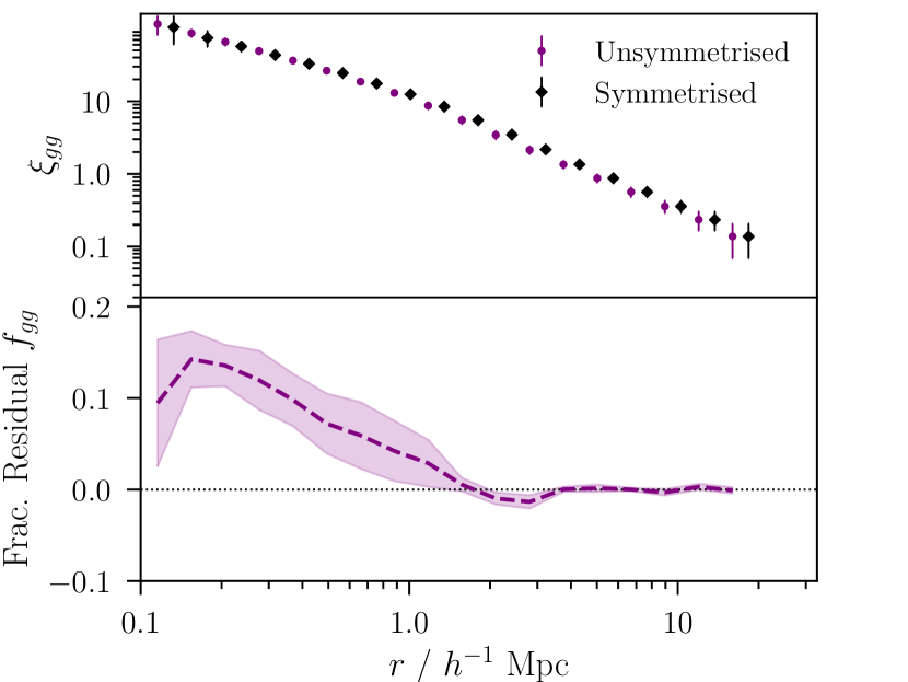
Figure 2: Upper panel: The galaxy-galaxy correlation function, as a function of three dimensional comoving separation before and after halo symmetrisation. The purple and black points are offset horizontally left and right by the same small interval to aid clarity. Lower panel: The fractional difference between the symmetrised and unsymmetrised measurements in the full sample, without satellite-central splitting. The shaded purple region shows the $1\sigma$ variance, as estimated by jackknife resampling the simulation volume.

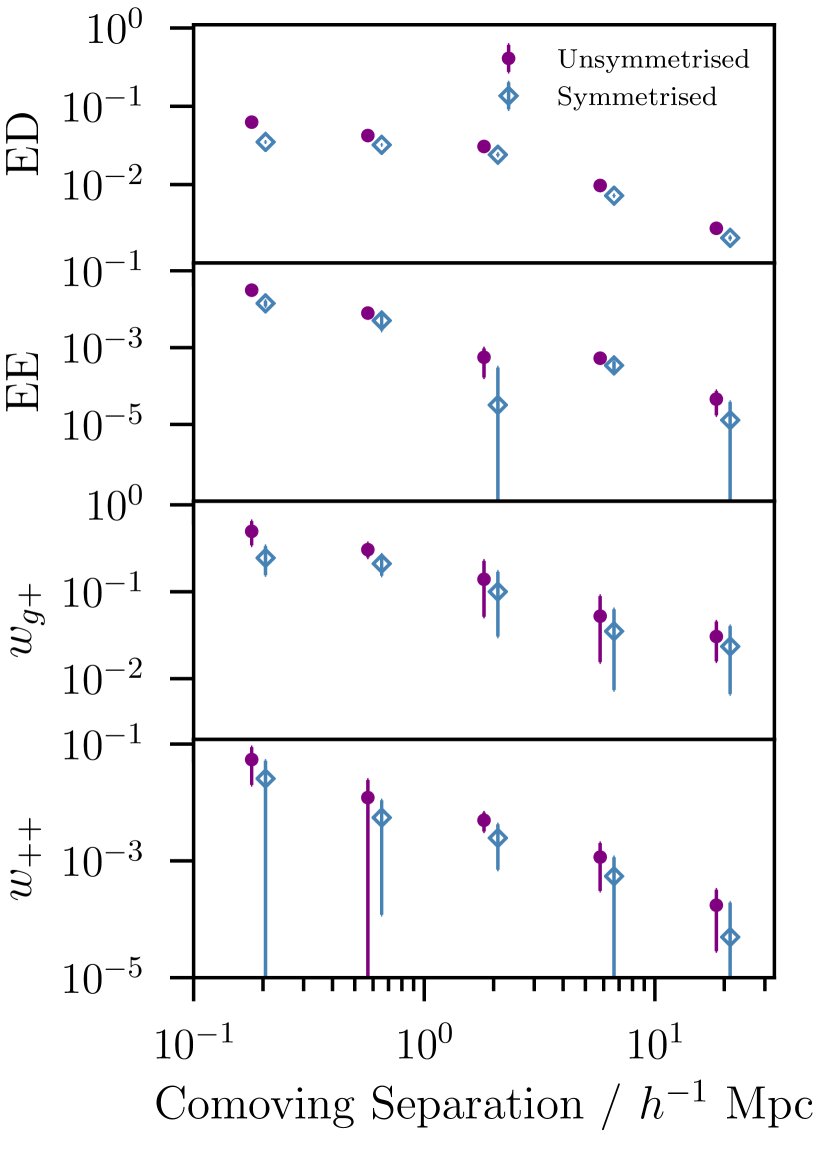
Figure 3: Two-point alignment correlation functions, as measured from our fiducial MassiveBlack-II galaxy catalogue. The horizontal axis shows the separation between galaxy pairs, either in three dimensional comoving space (in the case of EE and ED) or as projected into a plane perpendicular to the line of sight (for $w_{g+}$ and $w_{++}$). Purple filled points show measurements on the unsymmetrised catalogue, which includes the effects of halo anisotropy. The open blue points show the same measurements on an artificially symmetrised catalogue, in which satellite galaxies are spherically distributed around the centre of mass of their host halo. The four statistics shown here are defined algebraically in Section 3.

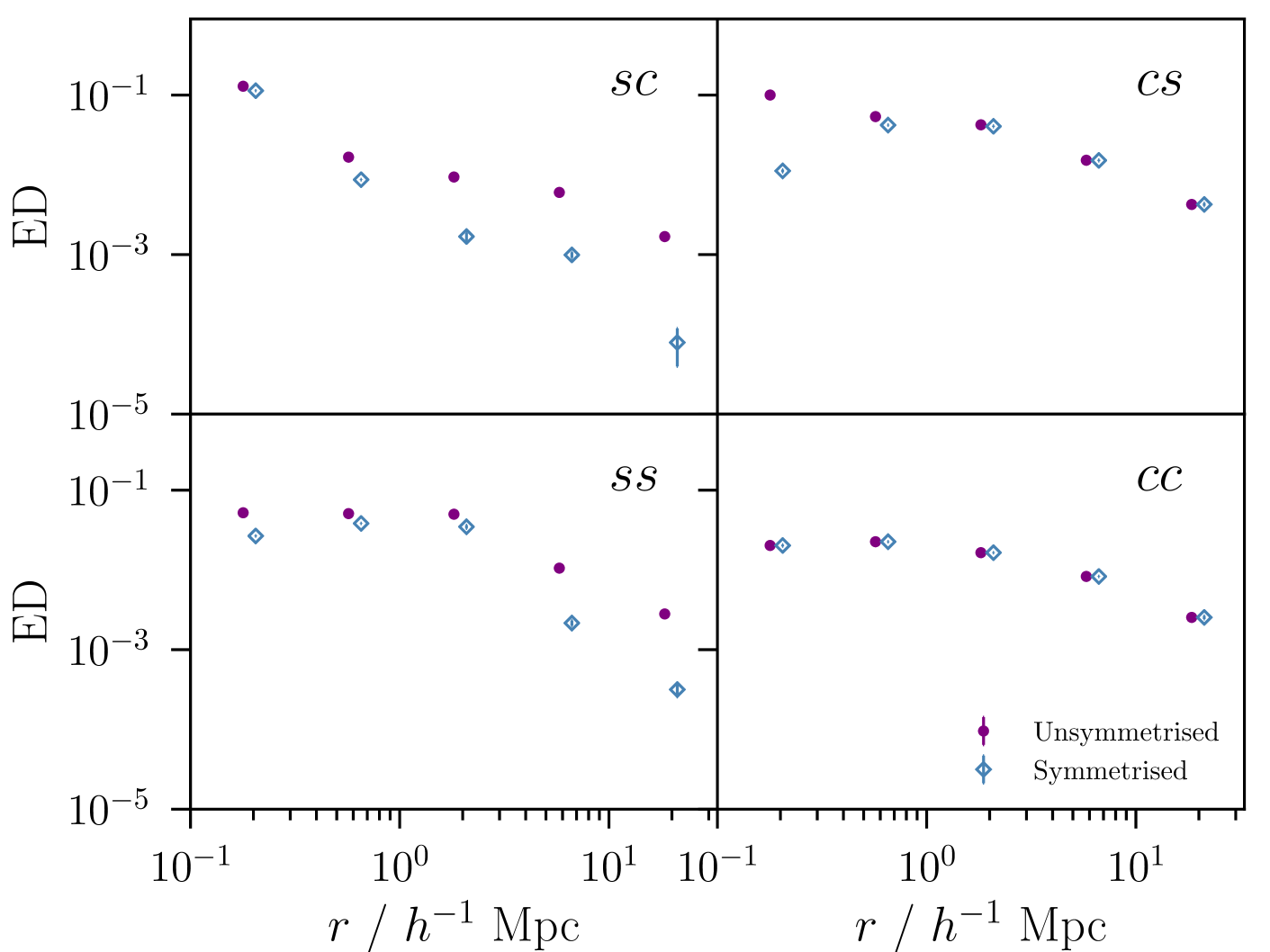
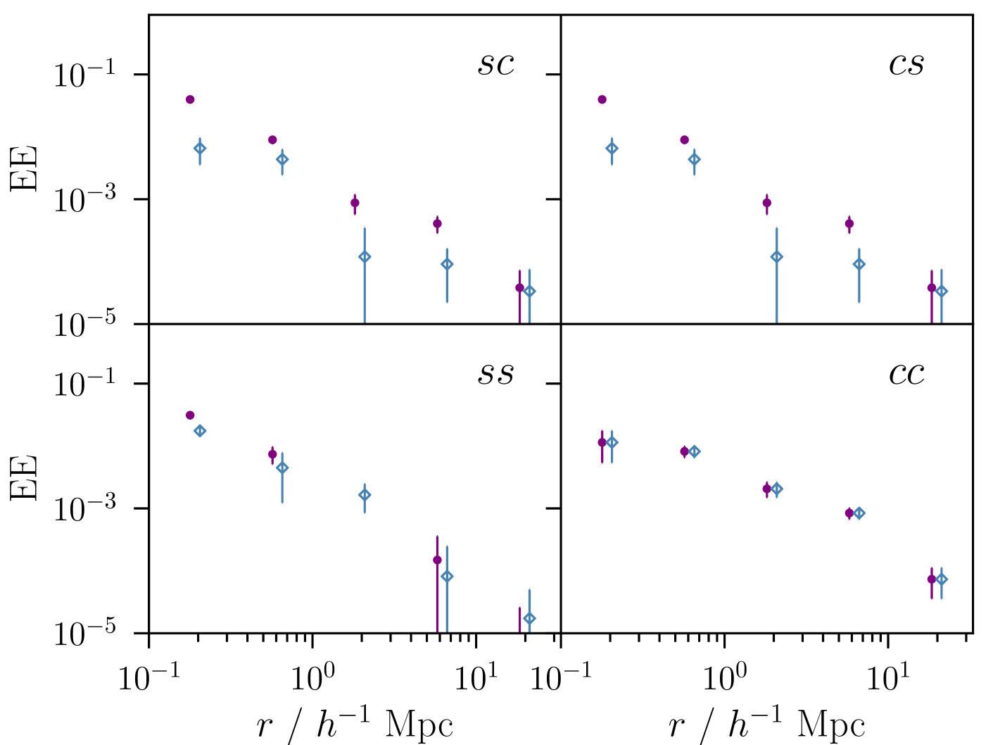
Figure 4: Three-dimensional alignment correlation functions, as measured within the MassiveBlack-II simulation volume before and after halo symmetrisation. The upper panel shows the two-point correlation of galaxy shapes and directions, while the lower shows the analogous shape-shape measurements. The definitions of these correlations can be found in Equations (8) and (9). All are shown as a function of comoving distance at redshift zero. Each of the four sub-panels shows a different combination of central and satellite samples (indicated by the letters in the top right; ED $sc$, for example, indicates the correlation of the shapes of central galaxies with the relative positions of satellites). In each case, the filled purple points show the fiducial unsymmetrised measurements and the open blue diamonds show the result of symmetrisation by rotating satellites within each halo about the dark matter centre of mass. Note that the third point in the EE $ss$ correlation is negative $(\sim-0.0012\pm 0.0008)$, and so not visible on a log scale.

As is clear from Figures 3 and 4 (and even more so in the additional measurements shown in Appendix A), lack of statistical power ensures the errorbars on virtually all of the correlation functions based on MassiveBlack-II are significant. Comparisons of the sort attempted here benefit at some level from the fact that the shape noise properties of the simulated dataset are largely unaffected by symmetrisation. Modulo low-level bin-shifting in the one-halo regime, then, one might expect the statistical significance of the difference between symmetrised and unsymmetrised correlation functions to be greater than that on either of the measurements in isolation. As discussed in the previous section, we seek to minimise the impact of noise by evaluating $f_{\alpha}$ using smooth fits rather than the measured correlation functions in the denominator of Equation (15). We show the fractional bias in the lower panel of Figure 5, along with the absolute residual in the upper panel.

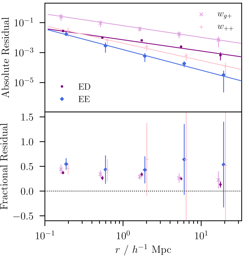
Figure 5: The contribution of halo anisotropy to various alignment correlation functions. Upper: the absolute difference between the two-point measurements made on the same simulation volume before and after halo symmetrisation. The solid lines show smooth power law fits to each residual. Lower: The fractional residual between symmetrised and unsymmetrised measurements, as estimated using power law fits to the unsymmetrised correlation function. The difference is defined such that $f=($symmetrised-unsymmetrised$)/$unsymmetrised, and so positive values indicate an increase in power at a particular scale relative to the idealised treatment with perfect spherical symmetry.

4.2 Robustness of Results

4.2.1 Central Flagging & Choice of Symmetrisation Pivot

In this section we seek to test the explicit choices made during the course of this analysis, with the aim of demonstrating the robustness of our results. The most obvious (and controllable) such choices regard the halo symmetrisation process; we chose to spin galaxies about the dark matter potential minimum. Similarly, the galaxies labelled as “centrals” are chosen by defining a fixed boundary at $0.1R$ and identifying the most massive galaxy within that sphere (see Section 2.3.2). This quantity has no clear mapping onto observables, and the correspondence to the objects classified as centrals in real data is non-trivial. We thus rerun our pipeline twice using slight modifications to these features. That is, we (a) perform the symmetrisation of satellites using the central galaxy of a halo as the pivot instead of the potential minimum and then (b) flag central galaxies by minimising the Euclidean distance from the potential minimum within each halo, rather than the more complicated definition described. The results are shown by the pink and green points (circles and filled diamonds) in Figure 6, which quantify the difference in anisotropy bias when switching to the modified analysis configuration.

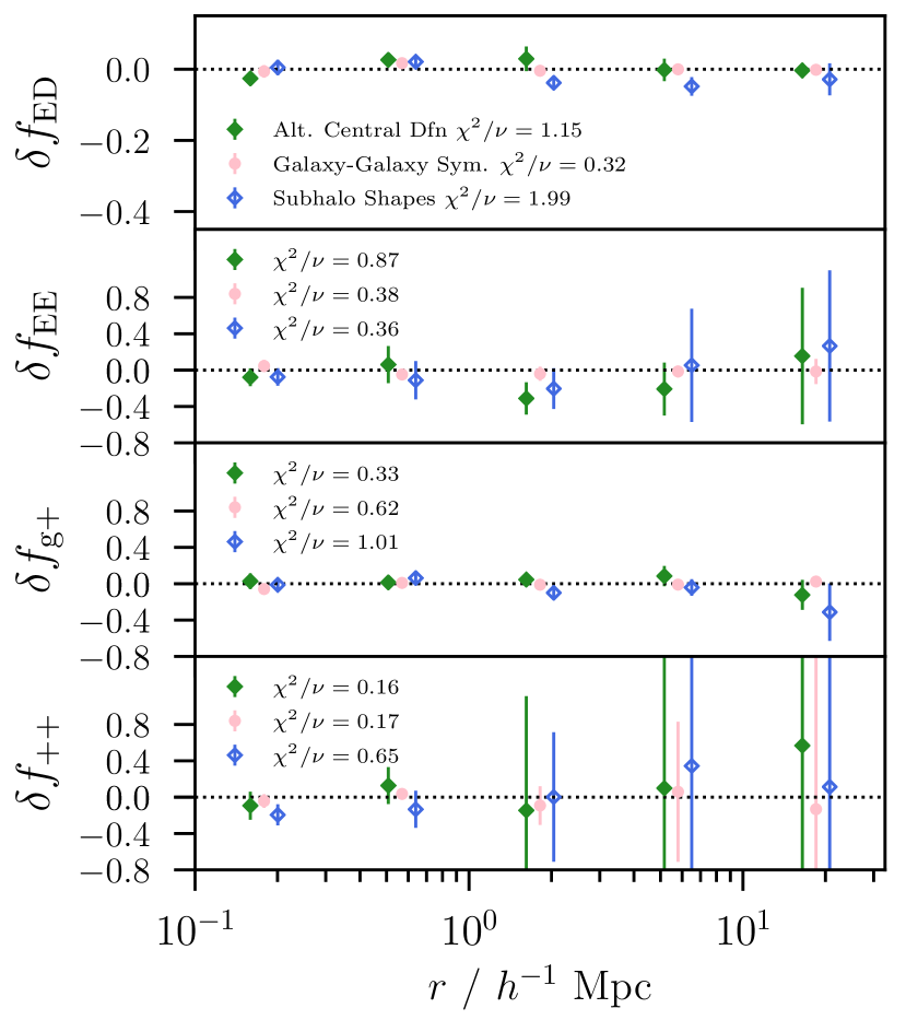
Figure 6: The change in the fractional anisotropy bias in the four alignment correlations discussed in this paper due to various analysis choices. The pink points show the shift due to symmetrising satellite galaxies about the central galaxy instead of the halo centre of mass. The filled green diamonds show the impact of using a simple geometric definition for “central” galaxies, as opposed to the combined definition (c) in Section 2.3.2. The open blue diamonds show the change induced by using ellipticities and orientations derived from the underlying dark matter subhalo of each galaxy instead of the visible component. The reduced $\chi^{2}/\nu$, where $\nu=5$ is the number of data points in the measurement, is shown in the legend for each measurement. A small horizontal offset is applied to the points in each bin to aid visibility.

As is apparent here, neither choice has a significant impact on our results. The reduced $\chi^{2}$ values, shown in each panel, give us no reason to suspect the deviations from zero are anything more systematic than statistical noise. We also test the impact of switching from the basic inertia tensor to a reduced version, wherein the stellar particles used to compute the moments of a subhalo are weighted by the inverse square of the radial distance from the centre of mass. This induces a more significant difference, at the level of $\delta f\sim-0.4$. The interpretation of this result is not totally straightforward. Dividing by the radial distance in effect imposes circular weighting, which will bias the resulting projected ellipticity low. Although the difference in the weight of the wings of a galaxy relative to its core impacts how strongly it is affected by symmetrisation, differences in the effective shape bias will also produce such effects. The magnitude and direction of the shift noted here is approximately the same as that seen across several mass bins by Tenneti et al. (2015a) (see their Fig. 5; compare black and blue solid lines). This, while not definitive, does suggest that other factors contributing to the difference in the $f_{\alpha}$ are likely subdominant to the shape bias.

4.2.2 Comparing MassiveBlack-II & Illustris

Though grouped under the umbrella term “hydrodynamical simulations”, the choices that go into building a dataset such as MassiveBlack-II can significantly affect its observable properties. A small handful of comparable simulations exist in the literature, most notably Horizon-AGN (Dubois et al., 2016), Illustris (Vogelsberger et al. 2014; and as of December 2018 also IllustrisTNG Nelson et al. 2018), EAGLE (Schaye et al., 2015) and cosmo-OWLS (Le Brun et al., 2014).

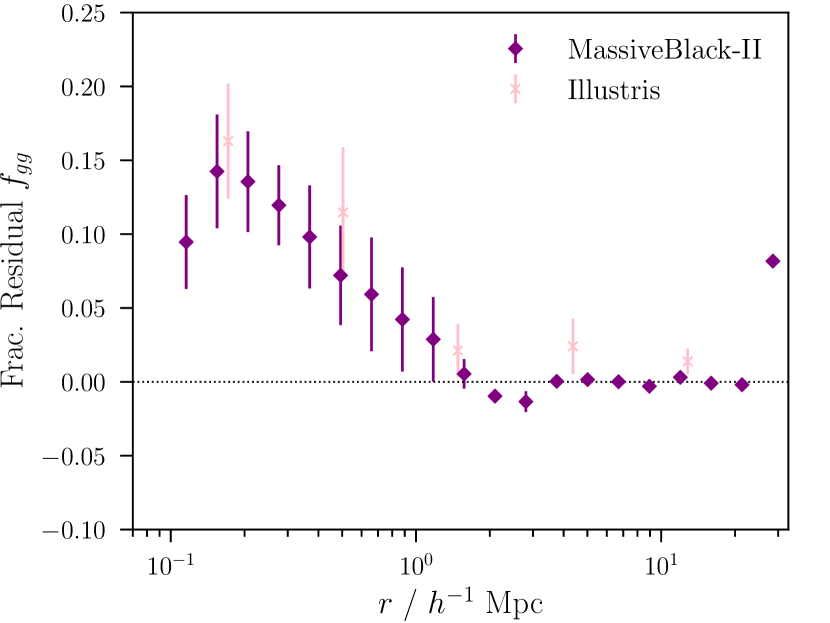
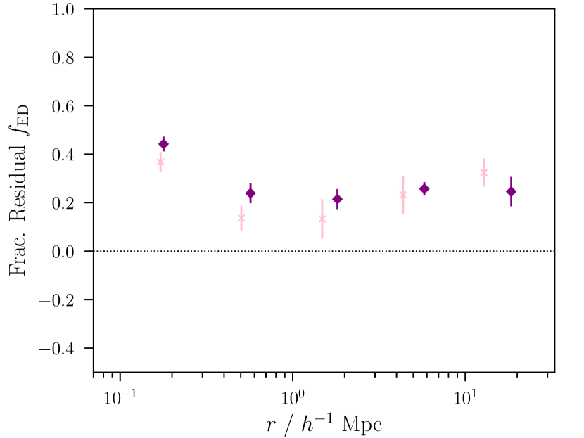
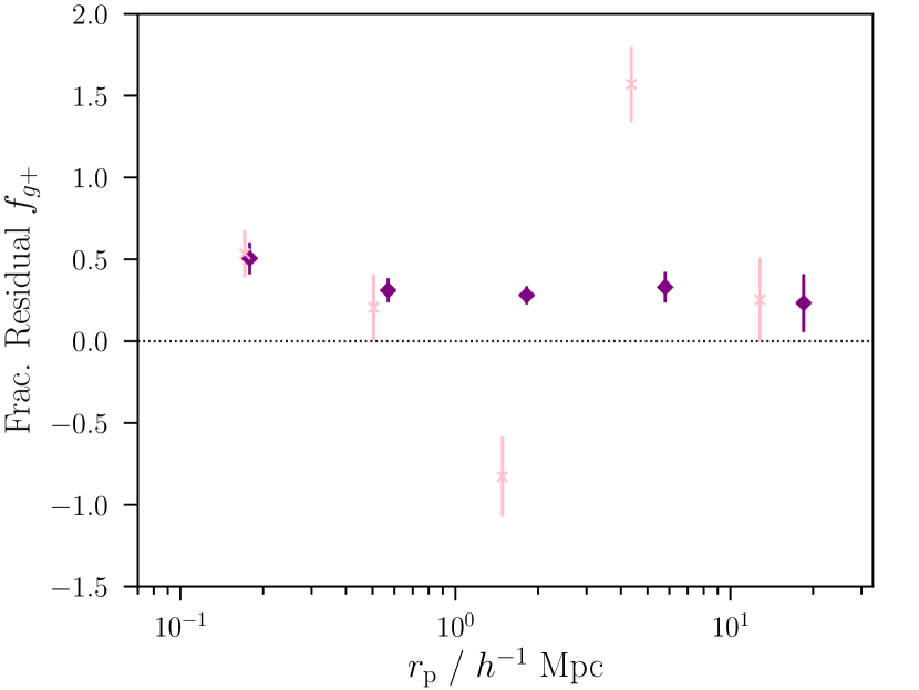
Figure 7: A comparison of anisotropy bias entering various correlation functions, as measured on the MassiveBlack-II and Illustris-1 galaxy catalogues. We show here (from top) 3D galaxy-galaxy, 3D ED and projected galaxy-tangential shape ($w_{g+}$). In each panel the purple diamonds indicate MassiveBlack-II, while the pink crosses show measurements based on Illustris-1. Note that we omit the EE and $w_{++}$ correlations here; though these measurements were made on Illustris-1, the signal-to-noise is sufficiently low as to make the comparison unenlightening.

In the recent past a number of studies have set out to explore the behaviour of intrinsic alignment between galaxies in these mock universes (see Codis et al. 2015a; Chisari et al. 2015; Velliscig et al. 2015; Tenneti et al. 2016; Chisari et al. 2016) with not entirely consistent results. Chisari et al. (2015), for example, report a dual IA mechanism in early-type and late-type galaxies, with the latter aligning tangentially about the former, and early-type (spheroidal) galaxies tending to point towards each other. Addressing the same question using the public MassiveBlack-II and Illustris data, however, Tenneti et al. (2016) find no such duality in either simulation. No conclusive answer has been provided as to why these datasets disagree, although there has been speculation (Chisari et al., 2016) that it is a product of differing prescriptions for small scale baryonic physics (see also Soussana et al. 2019, whose findings appear to support this idea). Similarly, it has been noted in Horizon-AGN that as the mass of the host halo declines, there is a transition from parallel alignment between galaxy spins and the direction of the closest filament to anti-alignment. Such a shift is expected based on observational data (Tempel & Libeskind, 2013), and tidal torque theory (Codis et al., 2015b), but has not been reported in MassiveBlack-II (Chen et al., 2015). More recently, and somewhat in tension with earlier results, Krolewski et al. 2019 report a transition from alignment to anti-alignment in dark matter subhalo shapes in both Illustris and MassiveBlack-II. Notably, in the former case a very similar sign flip is seen in stellar shapes, but this feature is not seen in the latter. Though we highlight the discrepancies here, it is worth bearing in mind that despite differing considerably in aspects of their methodology there is consistency between the bulk of IA measurements on hydrodynamical simulations, at least up to a constant amplitude offset.

Given that we have no prima facie reason to believe one simulation over another, we will consider such variation as a source of systematic uncertainty and seek to constrain it as best we can. To this end we apply our pipeline to the public Illustris-1 dataset. This requires some small changes in our treatment of cuts and periodic boundary conditions to account for differences in mass resolution and box size, but the comparison is otherwise straightforward. We show the fractional anisotropy bias in the resulting correlation functions in Figure 7.

The simplest case, that of galaxy-galaxy clustering, is shown in the upper left-hand panel. The two measurements are consistent to within statistical precision. It is worth bearing in mind here that we should not expect the two to be identical as the galaxy samples differ slightly in comoving number density and background cosmology. Within the bounds of our jackknife errorbars the impact of halo symmetrisation is likewise consistent in the IA correlations and enters on the same scales in the two datasets. Though one can see minor differences in the alignment correlation functions themselves (not shown here) our results do not indicate any clear discrepancy in the anisotropy bias between MassiveBlack-II and Illustris-1. There are known issues with the two simulations; the AGN feedback prescription in Illustris-1, for example, is known to overestimate the magnitude of the effect (Vogelsberger et al., 2014). Likewise the absolute alignment amplitude in MassiveBlack-II has been shown to be overpredicted relative to data (Tenneti et al., 2016). Such flaws affect the stellar mass function and other basic sample statistics but, notably, do not translate into differences in anisotropy bias.

4.2.3 Stellar vs Dark Matter Shapes

As discussed in Section 3.1, use of the stellar component for measuring galaxy shapes is a well-motivated analysis choice, observationally speaking; however advanced the measurement algorithm, we are constrained to measuring the shear field using luminous matter at the positions of galaxies. A natural question, however, is whether the intrinsic alignment signal (and indeed the anisotropy bias) imprinted in galaxy shapes accurately reflects the properties of the underlying dark matter subhalos. We test this by rerunning our measurements using orientations and ellipticities derived from the dark matter particles associated with each galaxy. The resulting shift $\delta f_{\alpha}$ is shown by the open blue points in Figure 6. For each statistic the reduced $\chi^{2}$ per degree of freedom is, again, shown in the legend. As with the other tests in this section we report no statistically significant shift. That is, though the raw alignment statistics measured with visible galaxy shapes and dark matter subhalo ellipticities differ, the aniosotropy bias does not. This is intuitively understandable, given that the positions and orientations of dark matter subhalos mirrors relatively closely that of visible satellite galaxies.

4.3 Dependence on Halo Mass

Though motivated by simulation convergence, the precise cuts applied to the fiducial catalogue $(n_{\mathrm{m}}<1000,n_{\mathrm{st}}<300$; see Section 2.3) are somewhat arbitrary. Given the constraints of the dataset (no ray-tracing or shape measurements, no reliable photometric fluxes, and galaxies sitting in a limited number of well-spaced redshift slices) constructing a realistic sample representative of a real lensing survey is not straightforward. One factor we can, however, test is the dependence on galaxy (subhalo) mass. This is useful in the sense that in real data the finite flux limit will in effect impose a lower mass cutoff at fixed redshift; if our results are robust to the exact cutoff, it suggests more general applicability in the practically useful context of a shape sample in a modern lensing survey.

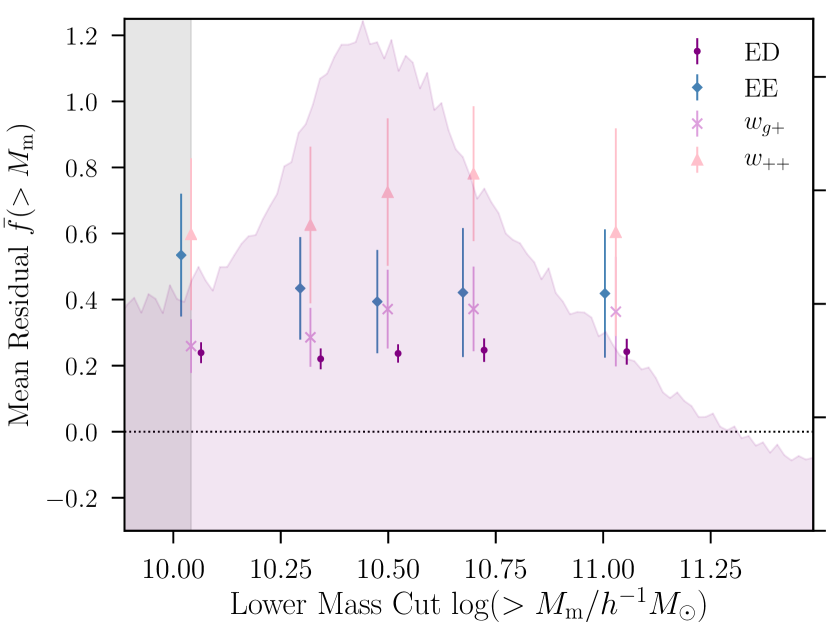
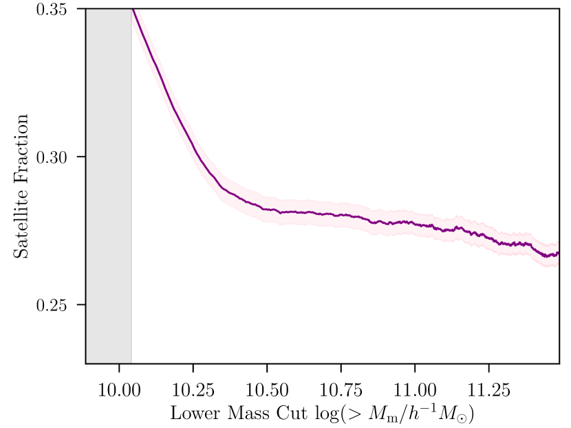
Figure 8: Upper panel: Fractional anisotropy bias as a function of the lower subhalo mass threshold applied to the catalogue. The different point styles show the four alignment statistics discussed in this work. In order to reduce $f_{\alpha}(r)$ into a single number, the measured fractional difference in the correlation functions is averaged on scales larger than $1h^{-1}$ Mpc, in which regime it is approximately constant. The grey shaded region corresponds to the fiducial cut at $1.1\times 10^{10}h^{-1}M_{\odot}$, or 1000 dark matter particles. Subhalos below this threshold are discarded to ensure convergence in the three dimensional inertia tensor calculations. A small horizontal offset has been applied to aid visibility. The underlain histogram shows the distribution of galaxy masses in the uncut catalogue. Lower panel: The variation in satellite fraction with lower mass cut. The purple line show the fiducial central flag definition and the shaded band shows the $1\sigma$ jackknife uncertainty.

To test this we construct a supersample of the fiducial catalogue with a lower dark matter mass cut (300 particles). The intrinsic alignment correlations are remeasured repeatedly with a series of increasing mass thresholds. The resulting fractional anisotropy biases are shown in the upper panel of Figure 8. The measurements here are designed to illustrate the evolution of the large scale anisotropy bias, and so are limited to scales larger than $1h^{-1}$ Mpc, where $f_{\alpha}$ is approximately constant (see the lower panel of Figure 5). The lack of a strong correlation here is worth remarking on; given the unrepresentative nature of our data, it offers some indication that our results might be applicable beyond this particular simulated galaxy sample.

To examine the evolution of the small scale anisotropy bias with halo mass we perform a similar exercise as the above; where before we averaged $f_{\alpha}(r)$ on large scales to obtain a single number, our summary statistic is now the best fitting power law slope $\partial\mathrm{ln}f/\partial\mathrm{ln}r$, fit on scales below $3h^{-1}$ Mpc. We have seen that the large scale amplitude of the anisotropy bias is relatively stable to the sample selection. The idea now is to test whether the shape of the scale dependent bias is similarly stable. This is shown in the left panel of Figure 9. In contrast to the previous result, we now see hints of a correlation. All four of the correlations show a gradual but consistent increase in the slope of the anisotropy bias as the mass threshold is raised. This can be interpreted as follows. There is evidence in the literature that the three dimensional dark matter distribution of massive halos tends to flatter that that of smaller halos (Jing & Suto, 2002; Springel et al., 2004; Allgood et al., 2006; Schneider et al., 2012). It follows, then, that the satellite distributions should be more concentrated at small azimuthal angles (also bourne out in the literature; see van den Bosch et al. 2016, Huang et al. 2016), and so the small scale ED $cs$ signal is stronger. This signal is strongly scale dependent, and is also washed out entirely by symmetrisation. This competes with ED $sc$ on small scales; in massive halos ED $cs$ makes up a larger fraction of the overall alignment signal, and so the anisotropy bias is exhibits a stronger scale dependence.

One can also think about the question in terms of one- and two-halo contributions. At high masses, the small scale anisotropy bias is dominated by intra halo central-satellite interactions, which fall off rapidly with separation. As the mass cut shifts downwards, one is preferentially including galaxies in low mass halos, which induces a net reduction of the mean satellite fraction. Since the host halos of low mass galaxies contain very few satellites, the impact of the symmetrisation process enters only at the level of two halo interactions, which scale more gradually with separation. This is true for both shape-shape and shape-position correlations.

The above arguments provide, at least in part, an explanation for the apparent mass dependence seen in Figure 9.

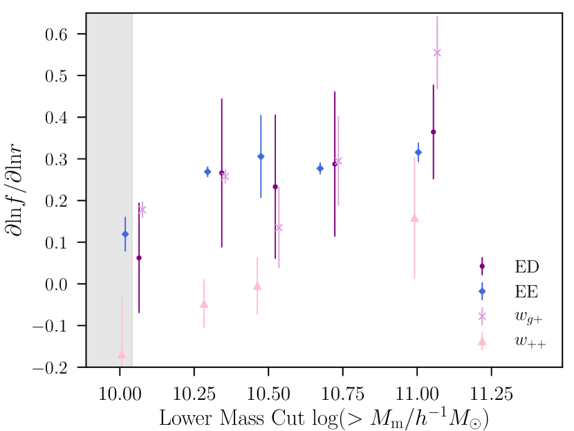
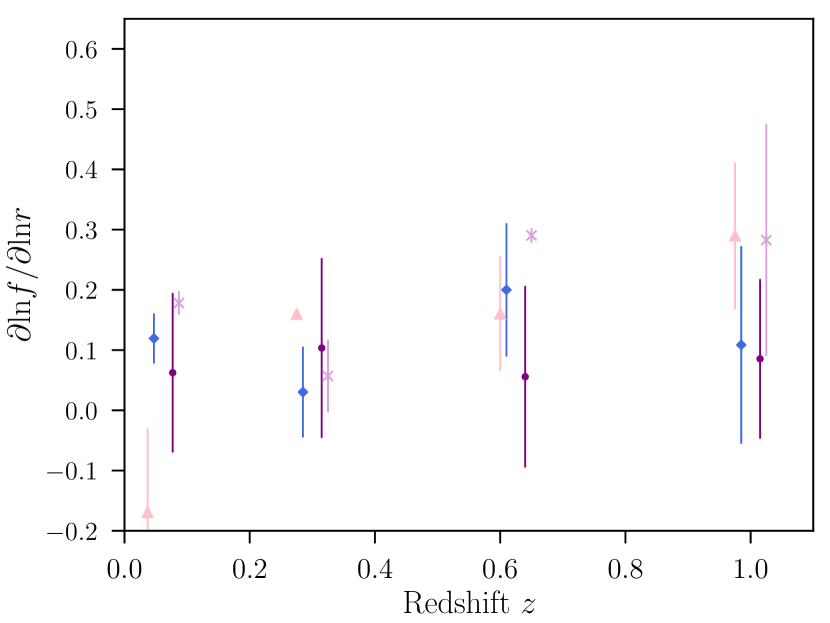
Figure 9: Gradient of the small scale fractional anisotropy bias $\partial\mathrm{ln}f(r)/\partial\mathrm{ln}r$, as a function of minimum subhalo mass (left) and of redshift (right). As above, the four point styles indicate different alignment correlations. The shaded band in the left-hand panel shows the fiducial mass cut used in this paper. Note that the points are slightly offset from each other along the horizontal axis to aid visibility.

4.4 Redshift Dependence

The results presented in the earlier sections of this paper are based exclusively on the lowest simulation snapshot, at $z=0.062$. We now explore how our findings change as one approaches redshifts more typically used for cosmic shear measurements.

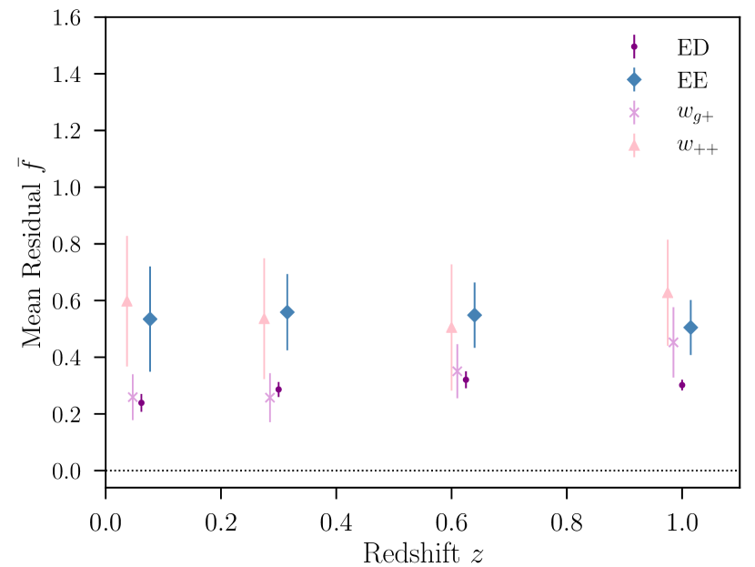
Figure 10: The redshift evolution of large scale anisotropy bias. Each bias point for a specific correlation function at given redshift is the mean over comoving scales larger than $1h^{-1}$ Mpc, where $f(r)$ is approximately constant. Note that we do not show binned values here; the discrete redshifts are defined by the four simulation snapshots (see Table 2) and are exact and known precisely, meaning the horizontal errorbar is effectively zero. The points at each redshift are offset slightly from one another along the x-axis to aid visibility.

The catalogue building and symmetrisation pipeline is applied independently to three snapshots at redshifts $z=[0.300,0.625,1.000]$, in addition to the fiducial dataset at $z=0.062$. Though this will not capture correlations between measurements at different redshifts, it allows us to make a simple comparison of the relative importance of satellite anisotropy in different epochs. The result is shown in Figure 10. Note that in order to condense a fractional anisotropy bias, naturally measured as a function of scale, into a single number we again average $f(r)$ on scales $r>1h^{-1}$ Mpc. This cut is intended to isolate the two-halo regime, within which the effect of symmetrisation is roughly constant. As before, our conclusions here are limited by the statistical power of the dataset. The ED correlation and, to a lesser extent, $w_{g+}$ do however offer a meaningful constraint. In these cases we find a potential weak positive redshift dependence over the range in question. Linear fits to the four points shown in Figure 10 give slopes of $m_{\mathrm{ED}}=0.05\pm 0.03$ and $m_{g+}=0.20\pm 0.03$ for ED and $w_{g+}$ respectively. No clear evolution is seen in $f_{\mathrm{EE}}$ and $f_{\mathrm{++}}$, though the error bars are also consistent with a moderate correlation (of either sign).

We also fit a power law to the small scale fractional anisotropy bias $f_{\alpha}(r|r<3h^{-1}$ Mpc$)$ at each redshift. This exercise is entirely analogous to the earlier test for dependence on the shape of $f(r)$ on the halo mass threshold. The result is shown in the right-hand panel of Figure 9. As in Figure 10, we see no evidence of coherent evolution in the scale dependence of the bias with redshift.

It is worth remarking here that the catalogue selection mask is applied independently in each redshift. That is, the composition of the sample changes between snapshots, and so apparent redshift dependence in the anisotropy bias can arise either from genuine evolution in a fixed set of objects or from differences in the ensemble properties of the galaxies surviving mass cuts. Disentangling these two effects would require access to MassiveBlack-II’s merger history (in order to track individual subhalos between snapshots) and is considered beyond the scope of the current analysis.

5 Implications for Cosmology

Though assessing the impact of symmetry on the alignment correlation functions is qualitatively useful for demonstrating a physical effect, it says nothing about the penalties for failing to model that effect. That is, what we ultimately wish to know is how biased would future cosmology surveys be were they to rely on a spherically symmetric model for intrinsic alignments. If a spherical model inaccurately describes reality, but does not significantly bias the cosmological information in small scale shear correlations, then most cosmologists would consider it sufficient. It is to this question we turn in the following section. To this end we perform a simulated likelihood analysis along the lines of Krause et al. (2017) using mock lensing data designed to mimic a future LSST-like lensing survey. The key ingredients are detailed below. Where it is necessary to assume a fiducial cosmology, we adopt the best fitting Planck 2018 $\Lambda$CDM constraints (Planck Collaboration, 2018), $\mathbf{p}_{\mathrm{cos}}=(\Omega_{\mathrm{m}},A_{\mathrm{s}},n_{\mathrm{s}},\Omega_{\mathrm{b}},h)=\\ (0.311,2.105\times 10^{-9},0.967,0.049,0.677)$.

5.1 Mock Cosmic Shear Data

We set up our synthetic data vector as follows. We first use the public Core Cosmology Library (CCL; Chisari et al. 2018a) to construct source redshift distributions. We assume eight redshift bins over the range $z=0.20-2.75$ with Gaussian photo-$z$ dispersion $\sigma_{z}=0.05$. In addition, we superpose Gaussian outlier islands centred on random points drawn from the initial smooth $p(z)$ in each bin. One should note that this is not a rigorous quantitative error prescription (though it is conceptually similar to the catastrophic outlier implementation of Hearin et al. 2010). The point, however, is to generate qualitatively realistic $p(z)$ with overlapping non-analytic tails, which may be salient when considering the impact of intrinsic alignments. The resulting distributions are shown in Figure 11. We then use the Boltzmann solver CAMB (Lewis et al., 2000) to generate a matter power spectrum at the fiducial cosmology. Nonlinear corrections are calculated using halofit (Takahashi et al., 2012). With the mock $p(z)$, this is propagated through the relevant Limber integrals to generate $C(\ell)$s and then Hankel transformed to correlation functions $\xi_{\pm}(\theta)$. To model the covariance of these data we use a public version of the CosmoLike ^, code (Krause & Eifler, 2017), assuming a constant shape dispersion $\sigma_{e}=0.25$ per bin and a total area of 18,000 square degrees. Given the limited aims of this exercise we consider a (real-space) Gaussian covariance matrix to be sufficient. Omitting higher-order covariance contributions (e.g. non Gaussian and super-sample terms, and the impact of survey masks; see Takada & Hu 2013; Krause et al. 2016; Barreira et al. 2018; Troxel et al. 2018b) is expected to translate into an underestimation of one’s sensitivity to the smallest scales. This in turn will reduce the impact of small-scale mismodelling. In this sense, the results presented in the following should be treated more as a lower bound on the possible bias than a rigorous numerical prediction.

To produce the intrinsic alignment contribution to these data we first compute the GI and II power spectra according to the NLA Model. This prescription is assumed to capture the large scale IA correlations well; we modify it on small scales using a simple procedure designed to mimic the impact of erroneously assuming halo symmetry. The measurements of $w_{g+}$ and $w_{++}$ on the simulations are transformed into IA power spectrum using the relation:

$$P_{\delta_{g}\mathrm{I}}(k)=-\int\mathrm{d}r_{\mathrm{p}}2\pi r_{\mathrm{p}}J_{2}(kr_{\mathrm{p}})w_{g+}(r_{\mathrm{p}}),$$ (17)

and analogously

$$P_{\mathrm{II}}(k)=\int\mathrm{d}r_{\mathrm{p}}2\pi r_{\mathrm{p}}\left[J_{0}(kr_{\mathrm{p}})+J_{4}(kr_{\mathrm{p}})\right]w_{++}\left(r_{\mathrm{p}}\right),$$ (18)

where $w_{++}$ and $w_{g+}$ are the (noisy) measured correlation functions from MassiveBlack-II and $J_{\nu}$ is a Bessel function of the first kind of order $\nu$ (see Appendix A of Joachimi et al. 2011 and Mandelbaum et al. 2011’s Equation 7). These spectra are computed twice: first using the unsymmetrised measurements of $w_{++}$ and $w_{g+}$, and then using shifted versions corresponding to the maximum difference allowed by the jackknife errorbars on $f_{++}$ and $f_{g+}$. This yields difference templates $\Delta P_{\mathrm{GI}}(k)$ and $\Delta P_{\mathrm{II}}(k)$, which are applied to the NLA GI and II power spectra generated from theory. Note that we use the templates derived from the lowest redshift snapshot to modify the IA spectra at all redshifts. Given the lack of systematic variation seen in Figures 9 and 10 we consider this a reasonable decision. The resulting modified power spectra are shown in Figure 12. It is worth reiterating here: these templates are not accurate prescriptions for small scale intrinsic alignment suitable for forward modelling, but simply a quantification of the maximum impact this systematic could have, given our results from the previous section.

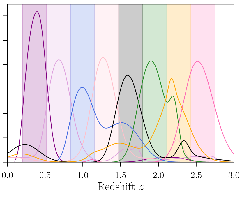
Figure 11: The mock photometric redshift distributions used in our simulated likelihood analysis. The sample is distributed among eight bins in the range $z=[0.20-2.75]$ with number densities ${\bf n}_{\mathrm{g}}=(3.3,3.1,3.0,1.5,1.5,1.0,0.5,0.5)$. The bounds of these bins are shown by the coloured bands.

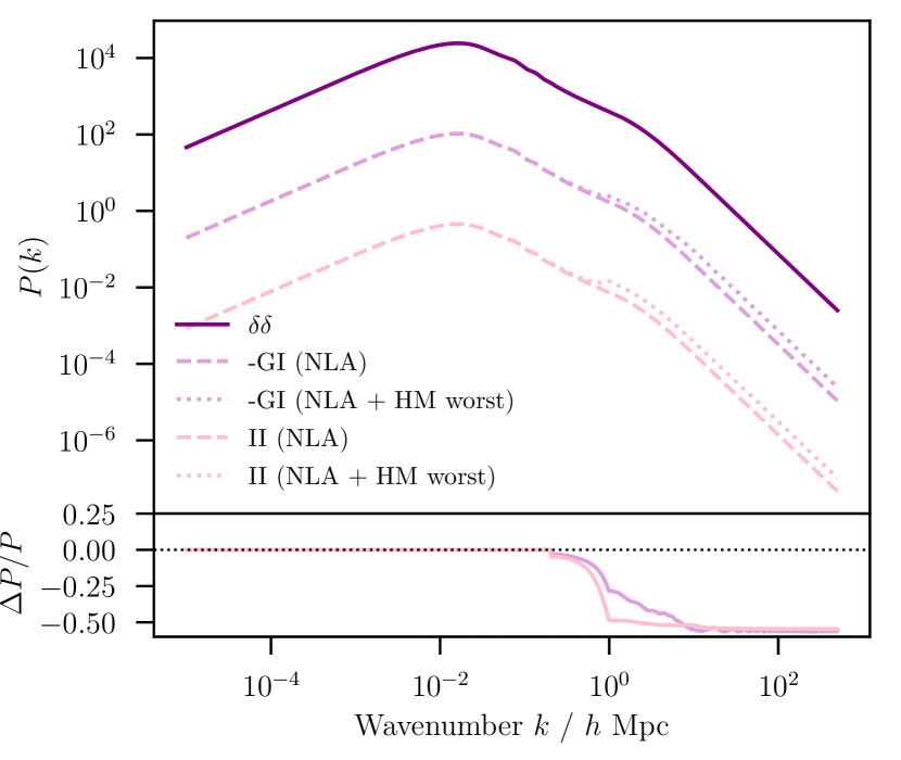
Figure 12: Theory power spectra at $z=0$ used for constructing our mock lensing data. The dashed lines show the baseline nonlinear alignment model prediction at the fiducial cosmology. The combined power spectra including a modification at high $k$ to account for the worst-case impact of assuming a spherical halo model are shown by the dotted lines. For reference we show the $z=0$ matter power spectrum at the same cosmology in purple (solid).

5.2 Simulated Likelihood Analysis

We perform a mock likelihood analysis on the contaminated data (constructed using the “NLA + HM Worst” spectra from Figure 12). The baseline analysis includes eighteen nuisance parameters, in addition to six cosmological parameters $\mathbf{p}_{\mathrm{cos}}=(A_{\mathrm{s}},n_{\mathrm{s}},\Omega_{\mathrm{m}},\Omega_{\mathrm{b}},h,w)$, following the broad methodology set out by Krause et al. (2017). We adopt priors, as set out in Table 4, which are designed to mimic the specifications of a future LSST-like lensing survey.

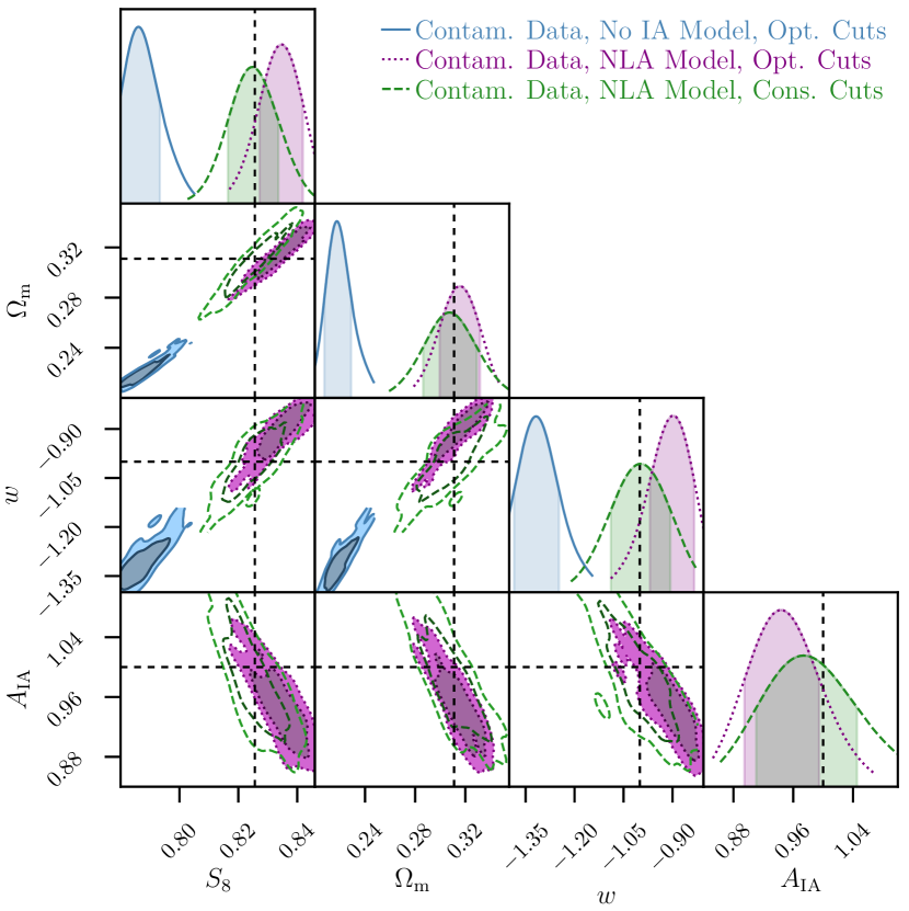
Figure 13: Constraints from artificially contaminated shear data, under different analysis configurations. The same mock data are used in all cases, modified in such a way to mimic the error caused by using a model for small scale IAs that neglects satellite anisotropy. The blue contours show a case in which no attempt is made to model intrinsic alignments (i.e. $A_{\mathrm{IA}}$ is fixed at zero). Purple show the same analysis, but also marginalising over a free IA amplitude and redshift power law index. In green (unfilled) we show the same result using stringent scale cuts, derived from baryonic simulations (discussed in Section 5.2), to mitigate the impact of the insufficient IA model on small scales.

Parameter	Prior	$\Delta p/\sigma_{p}$	$\Delta p/\sigma_{p}$
		(Conservative)	(Optimistic)
$A_{\mathrm{s}}$	$\mathrm{U}(1.1,3.0\times 10^{-9})$	$0.00(4)$	0.84
$n_{\mathrm{s}}$	$\mathrm{U}(0.5,1.5)$	$-0.29$	$-3.42$
$h$	$\mathrm{U}(0.4,0.9)$	0.18	$-1.60$
$\Omega_{\mathrm{m}}$	$\mathrm{U}(0.25,0.40)$	$-0.16$	0.22
$\Omega_{\mathrm{b}}$	$\mathrm{U}(0.01,0.10)$	$-0.11$	$-1.96$
$w$	$\mathrm{U}(-4.00,-0.33)$	$-0.01$	1.42
$\Omega_{\nu}h^{2}$	$\delta(0.0006155)$	0	0
$\Delta z^{i}$	$\mathcal{N}(0.001,0.01^{2})$	see text	see text
$m^{i}$	$\mathcal{N}(0.001,0.01^{2})$	see text	see text
$A_{\mathrm{IA}}$	$\mathrm{U}(-6,6)$	$-0.33$	$-1.38$
$\eta_{\mathrm{IA}}$	$\mathrm{U}(-6,6)$	$-0.13$	$-2.10$

Table 4: Priors and parameter biases derived from the mock analysis described in this section. The right-most two columns show the bias in the mean value of each parameter, as a fraction of the $1\sigma$ width of the marginalised $1\sigma$ posterior distribution, using two sets of scale cuts. The rows in the lower part of the table are nuisance parameters (from the top, photometric redshift error, shear calibration bias, intrinsic alignment amplitude and intrinsic alignment redshift power law index).

The matter power spectrum is computed at each point in parameter space using CAMB, with nonlinear modifications from halofit. To explore the posterior surface we use the emcee (Foreman-Mackey et al., 2013) Metropolis-Hastings algorithm, as implemented in CosmoSIS (Zuntz et al., 2015). To ensure the chains presented in this work are fully converged (after burn in) we apply the following criteria: (a) the parameter values, plotted in order of sampling, appear visually to be random noise about constant mean (i.e. with no residual direction or systematic variation in scatter) (b) if the chain is split into equal halves, the projected 1D posterior distributions evaulated using the two pieces do not significantly differ. Each of the chains used has a total of $1.5-2.0$ M samples, of which approximately fifteen percent survive burn in.

The intrinsic alignment signal is modelled using the two-parameter NLA model implemented by Troxel et al. (2018a), which differs from the input IA model due to the small-scale modifications described in the previous section. Note that this model includes a redshift scaling of the form $[(z+1)/(z_{0}+1)]^{-\eta_{\mathrm{IA}}}$, with a fixed pivot redshift $z_{0}=0.62$.

The scale cuts used in this analysis follow the basic methodology of Troxel et al. (2018a). That is, we compute our shear data vectors at a fiducial cosmology first using halofit alone, and then using the same matter power spectrum, but rescaled to mimic the most extreme scenario of baryonic feedback in a suite of OWLS AGN simulations (van Daalen et al., 2011). The minimum angular scale to use in our analysis for each correlation function is set to ensure the fractional difference in the two simulated versions of the data vector $|\Delta\xi^{ij}_{\pm}|/\xi^{\mathrm{halofit},ij}_{\pm}<0.01$. This value is calculated for each bin pair $ij$ and results in $\theta^{\mathrm{min}}_{+}=2.69$ arcminutes and $\theta^{\mathrm{min}}_{-}=39.91$ arcminutes in the uppermost auto-bin correlations of $\xi_{+}$ and $\xi_{-}$ respectively. For the purposes of forecasting, we will consider a second scenario in which more (but not all) of the shear-shear data are included. In this scenario, the minimum angular separation is rescaled such that $\theta^{\mathrm{min},ij}_{\pm}\rightarrow\frac{1}{4}\theta^{\mathrm{min},ij}_{\pm}$. In the analysis configuration described, with eight redshift bins and 50 angular bins per correlation, this increases the number of data points included in the analysis from 1252 to 1879. We refer to the two sets of scale cuts respectively as “conservative” and “optimistic” cases.

For reference, the first scenario we will consider is one in which we neglect to model the impact of IAs on any scale. With the contaminated data described above and the optimistic scale cuts, this results in the blue contours in Figure 13. Though it has been demonstrated elsewhere that neglecting IAs causes non-negligible parameter biases (Krause et al., 2016; Blazek et al., 2017; Troxel et al., 2018a), and this is clearly not a realistic analysis option, it is illuminating as a simple baseline case, with which to compare the size and direction of the biases in the following.

We next imagine a slightly more realistic scenario in which the optimistic cuts described above are employed. In this (purely hypothetical) setup, we assume that we can model baryonic physics and nonlinear structure formation perfectly; for small scale intrinsic alignments we imagine that we are using a halo model that assumes spherical symmetry, in a way analogous to the way halofit has been used for nonlinear growth in the past. This, again, is not an exact prescription but rather an illustration of the (potentially biased) information content of the small-scale shear correlations. The forecast results of such an analysis are shown by the solid purple contours in Figure 13. Unfortunately the small scale IA error in this scenario is sufficiently large to induce cosmological biases of $>1\sigma$ (see the “optimistic” column in Table 4). Most notably, we see shifts in the best constrained parameters $\Delta S_{8}=1.4\sigma$, $\Delta w=1.5\sigma$. Although such marginal shifts might be dismissed in comparison with other potentially larger systematics, it is worth bearing in mind that this is an idealised model. Indeed, for a single systematic, a $\sim 1\sigma$ shift is a non-trivial portion of the allowed error budget for an experiment like LSST. It is also worth remembering that this toy model neglects features such as non Gaussian covariances, which will increase rather than reduce sensitivity to small-scale mismodelling. Interestingly, in the 24 dimensional parameter space the bias is not entirely (or even predominantly) absorbed into the IA model; significant (several $\sigma$) compensatory shifts in the photo-$z$ nuisance parameters are seen, particularly in the lowest redshift bin. It is worth remarking here that this is precisely why interpretation of IA constraints is almost always non-trivial; the interplay with photo-$z$ error is often complex and one form of mismodelling can very easily mimic the other. We reiterate that IAs are being modelled here, but that the two-parameter NLA model neither matches the input IA signal exactly, nor is flexible enough to compensate fully for the discrepancy by absorbing it into an effective amplitude.

Finally, we consider the case in which IAs are again mismodelled, but in combination with more stringent set of scale cuts. Under such an analysis we obtain the green (unshaded) contours in Figure 13. The IA-induced parameter biases are seen to dwindle to semi-acceptable levels ($<1\sigma$, see the first column of Table 4). This result is reassuring, but somewhat expected, given that these cuts are conservative by construction, and designed to compensate for what is known to be an incomplete model of the physics entering the small scale matter power spectrum. One should note that the elimination (or, at least in large part, mitigation) of bias comes with a concurrent loss of cosmological information. The naive gain, evidenced by the visual comparison of the purple and green contours in Figure 13 in this case is relatively small. To more meaningfully assess the degradation in a multidimensional parameter space we evaluate the ratio $R=(|\mathbf{C}_{\mathrm{cos}}^{\prime}|^{0.5}-|\mathbf{C}_{\mathrm{cos}}|^{0.5})/|\mathbf{C}_{\mathrm{cos}}|^{0.5}$, where $\mathbf{C}_{\mathrm{cos}}$ and $\mathbf{C}^{\prime}_{\mathrm{cos}}$ are the $(6\times 6)$ covariance matrices of cosmological parameters from the two Monte Carlo chains. This gives a value of $R=17.7$, which is suggestive of a greater value in the small scales than suggested from the projected contours in Figure 13.

6 Discussion and Conclusions

We have used 113,560 galaxies from the MassiveBlack-II simulation to test the impact of halo anisotropy on the galaxy intrinsic alignment signal. MassiveBlack-II is one of a handful of high-resolution hydrodynamical simulations in existence to date and encompasses a comoving cubic volume of length $100h^{-1}$ Mpc. Using artificially symmetrised copies of the galaxy catalogues, we have found a reduction in power in the galaxy-galaxy correlation of a few percent on scales $\sim 1h^{-1}$Mpc, increasing to $\sim 10-15\%$ in the deep one-halo regime. We have shown the impact on alignment correlations to be significantly greater on all physical scales. Though our ability to quantify this effect is severely limited by the statistical precision afforded by the finite simulation volume, our results point to a difference in measured alignment correlations of the order of tens of percent or more, well into the two halo regime.

An IA model built on the assumption of spherical satellite distributions within dark matter halos would, then, underestimate the strength of both GI and II intrinsic alignment correlations considerably. This clearly has implications if we wish to use such a model to unlock the cosmological information on small scales in future lensing surveys, below the regime for which marginalising over an unknown amplitude parameter would be sufficient. We have described a series of robustness tests, designed to demonstrate the validity of our results beyond the immediate context of this analysis. To the best of our ability we have shown that our findings are independent of the various choices made in building our galaxy catalogues and the subsequent investigation based on them. In an additional, higher level, validation exercise we have also demonstrated that applying the same analysis pipeline to two different hydrodynamical simulations with different baryonic prescriptions yields consistent results within the level of statistical precision. We have further tested for dependence on redshift of this effect, and found no statistically significant variation across four snapshots in the range $z\in[0.062-1.000]$. Although this is shallower than contemporary lensing surveys, it is a sufficient range to allow detection of even a relatively slow systematic evolution were it to be present. Testing the impact of the lower dark matter mass cut of the galaxy sample, we have found no clear systematic change in anisotropy bias as the lower threshold is raised.

In a final strand of this analysis we have propagated the impact of halo anisotropy into a set of mock cosmic shear data. These simulated data are “contaminated” in such a way to mimic the impact of mismodelling the intrinsic alignment signal using a spherically symmetric halo model. Assuming a lensing survey with LSST-like number densities, and applying optimistic scale cuts, somewhat looser than those used in the Dark Energy Survey Y1 cosmic shear cosmology analysis, we have found biases in $S_{8}$ and $w$ of $1.4\sigma$ and $1.5\sigma$ respectively. Adopting more stringent cuts following the prescription of DES Y1 (adjusted for differences in the redshift distributions) the cosmological bias is seen to reduce to less than $1\sigma$ on all parameters, but at the cost to the volume of the constraints in the six dimensional cosmological parameter space of a factor $R=17.7$. It is worth noting that this is a simplified toy model scenario, intended to illustrate the effects of intrinsic alignment mismodelling alone.

Though the analysis presented here focuses on cosmic shear, $\xi_{+}$ and $\xi_{-}$ are not the only statistics affected by IAs. Future cosmology studies will likely use shear as part of a joint analysis alongside galaxy-galaxy lensing and, potentially, cluster lensing. The extrapolation of our findings to such an analysis is non-trivial, and a more comprehensive forecasting project would be required to quantify the impact of halo anisotropy. Given the scope of this paper, however, it is sufficient to demonstrate that modelling errors of this sort induce a non-negligible cosmological bias for at least one commonly used cosmological probe. Our analysis does not include non Gaussian (trispectrum) contributions to the covariance matrix, which become significant on small scales. This will affect the exact size of the biases presented in the previous section, but is not expected to alter the broad conclusions of the work.

It is also worth bearing in mind that a number of other poorly understood effects become relevant on the smallest scales, including nonlinear growth, baryonic feedback and beyond first-order galaxy bias. Even if one were to build a sufficiently accurate small scale IA model, advances must be made in modelling or mitigating these other systematics if we are to successfully access the information in small scale shear and galaxy-galaxy lensing correlations. Moreover, even given accurate models for all small scale effects, it is quite possible that parameter degeneracies would emerge that mimic power in the small scale intrinsic alignment correlations. As with all high-dimensional inference problems, this is a complicated subject that requires careful consideration before any cosmological analysis that includes small angular scales can proceed.

7 Acknowledgements

The authors would like to thank François Lanusse, Hung-Jin Huang, Duncan Campbell and Aklant Bhowmick for useful conversations and help with data access. We would also like to thank our anonymous referee for their thoughts on the work. Catalogue building and processing were performed using the Coma HPC cluster, which is hosted by the McWilliams Center for Cosmology, Carnegie Mellon University. The smoothed contours in Figure 13 were generated using chainconsumer (Hinton, 2016). This research is supported by the US National Science Foundation under Grant No. 1716131.

Appendix A Additional Alignment Correlation Functions

In this appendix we present some additional correlation functions; these were not included in the main body of the paper due to the low signal-to-noise of the measurements and qualitative agreement with their (simpler) ED and EE counterparts. They are shown in Figure 14 for completeness.

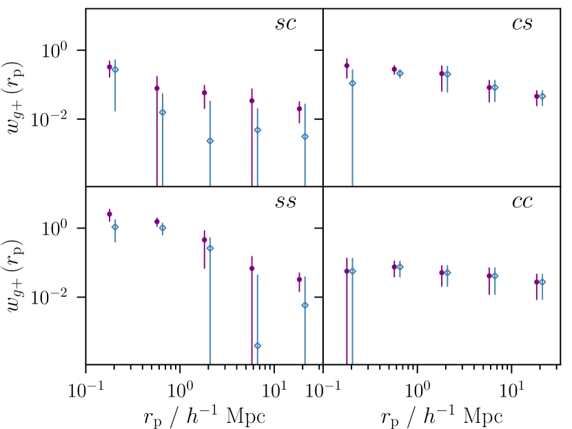
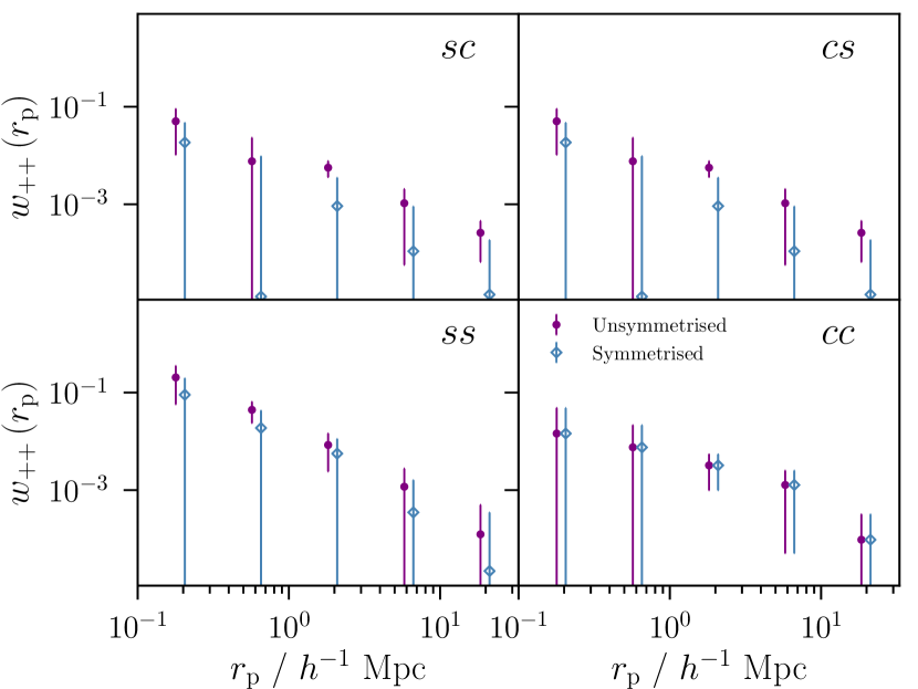
Figure 14: Projected alignment correlation functions, as measured within the MassiveBlack-II simulation volume before and after halo symmetrisation. The two panels show (left) galaxy-shape and (right) shape-shape measurements as a function of comoving separation perpendicular to the line of sight. Each of the four sub-panels shows a different combination of central and satellite samples. In each case, the purple dots show the fiducial unsymmetrised measurements and the open blue diamonds show the result of symmetrisation by rotating satellites within each halo about the dark matter potential minimum.

As in the EE case, $w_{++}$ is symmetric, and as such the two upper panels of the bottom section of this figure are identical by construction. Likewise, the purple and blue points in the $cc$ (bottom right) panels are numerically identical (since symmetrisation leaves the positions and shapes of central galaxies unchanged).

Appendix B An Algorithm for Isotropising Three Dimensional Positions

The task of isotropising objects in three dimensional space, though apparently trivial at first glance, is very easy to mishandle. Beyond the mathematics of the per-object rotation itself, one must be careful that the rotation itself does not imprint some preferred direction in the resulting distribution of object positions. Defining a random rotation axis direction $\phi,\theta$ and a random rotation about that axis $\alpha$, will leave one with a non-isotropic distribution of points (since the process favours small rotation angles). This is true even if $\phi$ and $\theta$ are correctly defined $\theta=2\pi u_{2}$ and $\phi=\arccos(2u_{1}-1)$, where $u_{1}$ and $u_{2}$ are random draws from uniform distributions $u_{i}\in[0,1]$. In the following we present a recipe for transforming a distribution of points with some preferred direction into an isotropic distribution about a centroid position $\mathbf{r}_{\mathrm{cent}}$.

As described in the main text of this paper, we first define a new position $\mathbf{r}^{\prime}=(R,\phi^{\prime},\theta^{\prime})$, where $\phi^{\prime}$ and $\theta^{\prime}$ are drawn from the distribution $U(0,2\pi)$. From these two positions, prior to and post rotation, one can calculate an orthogonal three vector

$$\mathbf{V}=\mathbf{r}\times\mathbf{r}^{\prime}/N,$$ (19)

where $N=|\mathbf{r}\times\mathbf{r}^{\prime}|$ is a normalisation constant. This defines a axis, about which a rotation can be defined to carry a point from $\mathbf{r}$ to position $\mathbf{r}^{\prime}$. That angle in the two dimensional plane defined by $\mathbf{r}$ and $\mathbf{r}^{\prime}$ is given by

$$\alpha=\arccos\left(\frac{\mathbf{r}\cdot\mathbf{r}^{\prime}}{|\mathbf{r}||\mathbf{r}^{\prime}|}\right).$$ (20)

with the vector $\mathbf{V}=(v_{x},v_{y},v_{z})$ and angle $\alpha$ we have the ingredients necessary to construct a rotation matrix. In three dimensions this is given by:

$$\mathbf{R}_{\theta}=\left(\begin{matrix}\cos\alpha+u_{x}u_{x}(1-\cos\alpha)\;\;\;\;\;u_{x}u_{y}(1-\cos\alpha)-u_{z}\sin\alpha\;\;\;\;\;u_{x}u_{z}(1-\cos\alpha)+u_{y}\sin\alpha\\ u_{y}u_{x}(1-\cos\alpha)+u_{z}\sin\alpha\;\;\;\;\;\cos\alpha+u_{y}u_{y}(1-\cos\alpha)\;\;\;\;\;u_{y}u_{z}(1-\cos\alpha)-u_{x}\sin\alpha\\ u_{z}u_{x}(1-\cos\alpha)-u_{y}\sin\alpha\;\;\;\;\;u_{z}u_{y}(1-cos\alpha)+u_{x}\sin\alpha\;\;\;\;\;\cos\alpha+u_{z}u_{z}(1-\cos\alpha)\\ \end{matrix}\right)$$ (21)

This rotation matrix can then be applied identically to rotate the shape vectors of a galaxy, such that the orientation relative to the centre of rotation is maintained: $\mathbf{a}^{\prime}=\mathbf{R}_{\theta}\cdot\mathbf{a}$. An implementation of this algorithm and simple numerical examples of its application can be found at https://github.com/McWilliamsCenter/ia_modelling_public.

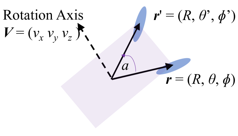
Figure 15: Schematic diagram illustrating the symmetrisation algorithm described in Appendix B, as applied to a single galaxy. The galaxy with initial position $\mathbf{r}$ (the right-most blue oval) is assigned a new position $\mathbf{r}^{\prime}$ at the same distance from the halo centre. The two position vectors $\mathbf{r}$ and $\mathbf{r}^{\prime}$ define a rotation angle $\alpha$ in their two dimensional plane (shown in purple) and an orthogonal rotation axis $\mathbf{V}$. These in turn can be used to calculate the rotation matrix that describes the mapping between the old and the new positions.

Appendix C Impact of Finite Simulation Volume

It is widely recognised in the literature that for a cosmological simulation of finite volume, measurements on certain scales are unreliable. In general, the imposition of a sharp cutoff at the edges of the box is equivalent to systematically cutting out small-$k$ modes; on the largest scales, then, we expect to see a deficit in power in the measured two-point functions. In this work, in order to mitigate the impact of this effect, we adopt a maximum scale of $r_{\mathrm{p}}=33h^{-1}$ Mpc, or a third of the MassiveBlack-II box length. We test the validity of this choice as follows: theory IA and galaxy clustering power spectra are first generated using CAMB at a fiducial cosmology. We then truncate those power spectra at a given $k_{\mathrm{min}}$, before propagating them through the appropriate Bessel integrals to given theory predictions for $w_{g+}$, $w_{++}$ and $w_{gg}$. The difference between these theory correlation functions with a $k_{\mathrm{min}}$ corresponding to the simulation box size, and those extending to $k=10^{-5}h^{-1}$ Mpc then gives us an estimate for the impact of this truncation on different projected scales. The results for the lowest redshift snapshot are shown in Figure 16.

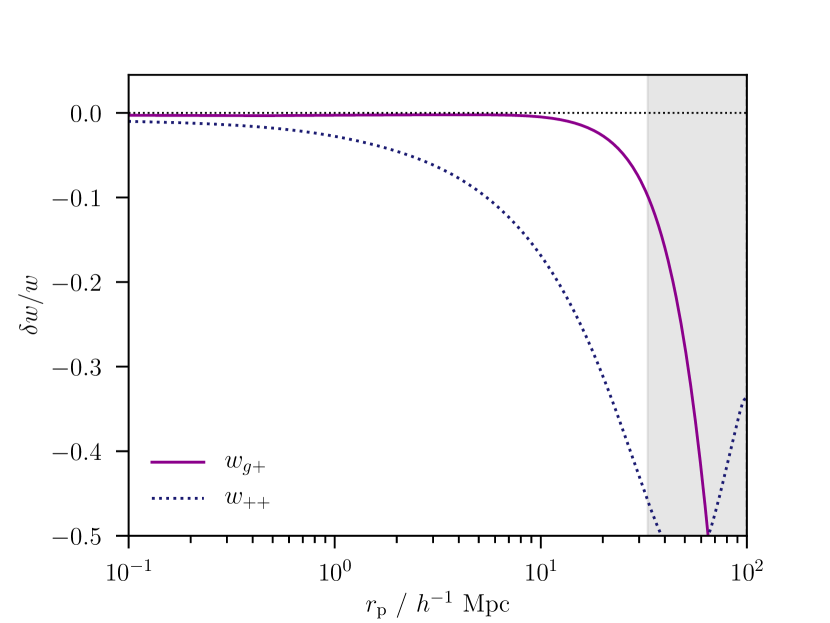
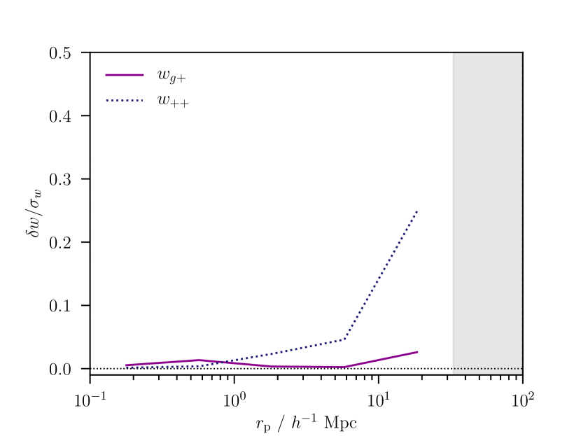
Figure 16: Upper: Fractional change in the projected correlation functions due to truncation at $k_{\rm min}=2\pi/100h^{-1}$ Mpc. The grey shaded region shows the scales discarded in this analysis. The sign convention here is such that negative values translate into a suppression of power in the truncated measurement. Lower: The change as a fraction of the jackknife $1\sigma$ error on each correlation function, as measured from MassiveBlack-II.

The three coloured lines here show the three different types of correlation function. Naturally, given that they have different Bessel kernels, we expect the scales on which the truncation impacts to differ slightly. As one might expect, the impact of the missing $k$ modes is to suppress the correlation functions, and the impact is greatest on the largest scales. Strikingly, due to the Bessel kernels used in converting the $++$ correlation into physical space, the impact is relatively large even on scales $\sim$ a few Mpc. The impact on $w_{g+}$ appears to be significantly smaller, at the level of one percent or less on scales $r_{\mathrm{p}}<33h^{-1}$ Mpc.

That the impact is clearly non-vanishing is not greatly surprising, given the relatively small box size of MassiveBlack-II. It is, however, reassuring that the suppression of the both IA correlation functions is comfortably less than the $1\sigma$ error bar on all scales considered.

References

- Agustsson & Brainerd (2010) Agustsson I., Brainerd T. G., 2010, ApJ, 709, 1321
- Allgood et al. (2006) Allgood B., Flores R. A., Primack J. R., Kravtsov A. V., Wechsler R. H., Faltenbacher A., Bullock J. S., 2006, MNRAS, 367, 1781
- Bagla et al. (2009) Bagla J. S., Prasad J., Khandai N., 2009, MNRAS, 395, 918
- Bailin & Steinmetz (2005) Bailin J., Steinmetz M., 2005, ApJ, 627, 647
- Bailin et al. (2008) Bailin J., Power C., Norberg P., Zaritsky D., Gibson B. K., 2008, MNRAS, 390, 1133
- Barreira et al. (2018) Barreira A., Krause E., Schmidt F., 2018, J. Cosmology Astropart. Phys., 6, 015
- Bernstein et al. (2016) Bernstein G. M., Armstrong R., Krawiec C., March M. C., 2016, MNRAS, 459, 4467
- Blazek et al. (2015) Blazek J., Vlah Z., Seljak U., 2015, J. Cosmology Astropart. Phys., 8, 015
- Blazek et al. (2017) Blazek J., MacCrann N., Troxel M. A., Fang X., 2017, arXiv e-prints, p. arXiv:1708.09247
- van den Bosch et al. (2016) van den Bosch F. C., Jiang F., Campbell D., Behroozi P., 2016, MNRAS, 455, 158
- Bridle & King (2007) Bridle S., King L., 2007, New Journal of Physics, 9, 444
- Bridle et al. (2010) Bridle S., et al., 2010, MNRAS, 405, 2044
- Butsky et al. (2016) Butsky I., et al., 2016, Monthly Notices of the Royal Astronomical Society, 462, 663
- Catelan et al. (2001) Catelan P., Kamionkowski M., Blandford R. D., 2001, MNRAS, 320, L7
- Chen et al. (2015) Chen Y.-C., et al., 2015, MNRAS, 454, 3341
- Chisari et al. (2015) Chisari N., et al., 2015, MNRAS, 454, 2736
- Chisari et al. (2016) Chisari N., et al., 2016, MNRAS, 461, 2702
- Chisari et al. (2017) Chisari N. E., et al., 2017, MNRAS, 472, 1163
- Chisari et al. (2018a) Chisari N. E., et al., 2018a, arXiv e-prints, p. arXiv:1812.05995
- Chisari et al. (2018b) Chisari N. E., et al., 2018b, MNRAS, 480, 3962
- Codis et al. (2015a) Codis S., et al., 2015a, MNRAS, 448, 3391
- Codis et al. (2015b) Codis S., Pichon C., Pogosyan D., 2015b, MNRAS, 452, 3369
- Crittenden et al. (2001) Crittenden R. G., Natarajan P., Pen U.-L., Theuns T., 2001, ApJ, 559, 552
- van Daalen et al. (2011) van Daalen M. P., Schaye J., Booth C. M., Dalla Vecchia C., 2011, MNRAS, 415, 3649
- van Daalen et al. (2012) van Daalen M. P., Angulo R. E., White S. D. M., 2012, MNRAS, 424, 2954
- Dark Energy Survey Collaboration (2016) Dark Energy Survey Collaboration 2016, Phys. Rev. D, 94, 022001
- Dark Energy Survey Collaboration (2017) Dark Energy Survey Collaboration 2017, Phys. Rev. D, 98, 043526
- Di Matteo et al. (2012) Di Matteo T., Khandai N., DeGraf C., Feng Y., Croft R. A. C., Lopez J., Springel V., 2012, ApJ, 745, L29
- Drlica-Wagner et al. (2018) Drlica-Wagner A., et al., 2018, ApJS, 235, 33
- Dubois et al. (2016) Dubois Y., Peirani S., Pichon C., Devriendt J., Gavazzi R., Welker C., Volonteri M., 2016, MNRAS, 463, 3948
- Dvornik et al. (2018) Dvornik A., et al., 2018, MNRAS,
- Faltenbacher et al. (2007) Faltenbacher A., Li C., Mao S., van den Bosch F. C., Yang X., Jing Y. P., Pasquali A., Mo H. J., 2007, The Astrophysical Journal Letters, 662, L71
- Fedeli (2014) Fedeli C., 2014, J. Cosmology Astropart. Phys., 4, 028
- Foreman-Mackey et al. (2013) Foreman-Mackey D., Hogg D. W., Lang D., Goodman J., 2013, PASP, 125, 306
- Hearin et al. (2010) Hearin A. P., Zentner A. R., Ma Z., Huterer D., 2010, ApJ, 720, 1351
- Hearin et al. (2017) Hearin A. P., et al., 2017, doi.org/10.5281/zenodo.835898 AJ, 154, 190
- Heymans et al. (2006) Heymans C., et al., 2006, MNRAS, 368, 1323
- Hinton (2016) Hinton S., 2016, JOSS 10.21105/joss.00045
- Hirata & Seljak (2004) Hirata C. M., Seljak U., 2004, Phys. Rev. D, 70, 063526
- Huang et al. (2016) Huang H.-J., Mandelbaum R., Freeman P. E., Chen Y.-C., Rozo E., Rykoff E., Baxter E. J., 2016, MNRAS, 463, 222
- Huang et al. (2018) Huang H.-J., Mandelbaum R., Freeman P. E., Chen Y.-C., Rozo E., Rykoff E., 2018, MNRAS, 474, 4772
- Huff & Mandelbaum (2017) Huff E., Mandelbaum R., 2017, preprint, (arXiv:1702.02600)
- Jarvis et al. (2004) Jarvis M., Bernstein G., Jain B., 2004, MNRAS, 352, 338
- Jing & Suto (2002) Jing Y. P., Suto Y., 2002, ApJ, 574, 538
- Joachimi et al. (2011) Joachimi B., Mandelbaum R., Abdalla F. B., Bridle S. L., 2011, A&A, 527, A26
- Joachimi et al. (2013) Joachimi B., Semboloni E., Hilbert S., Bett P. E., Hartlap J., Hoekstra H., Schneider P., 2013, MNRAS, 436, 819
- Joachimi et al. (2015) Joachimi B., et al., 2015, Space Sci. Rev., 193, 1
- Johnston et al. (2007) Johnston D. E., Sheldon E. S., Tasitsiomi A., Frieman J. A., Wechsler R. H., McKay T. A., 2007, ApJ, 656, 27
- Joudaki et al. (2018) Joudaki S., et al., 2018, MNRAS, 474, 4894
- Kasun & Evrard (2005) Kasun S. F., Evrard A. E., 2005, ApJ, 629, 781
- Kennicutt (1998) Kennicutt R. C., 1998, ApJ, 498, 541
- Khandai et al. (2015) Khandai N., Di Matteo T., Croft R., Wilkins S., Feng Y., Tucker E., DeGraf C., Liu M.-S., 2015, MNRAS, 450, 1349
- Kiessling et al. (2015) Kiessling A., et al., 2015, Space Sci. Rev., 193, 67
- Kilbinger (2015) Kilbinger M., 2015, Reports on Progress in Physics, 78, 086901
- Kirk et al. (2015) Kirk D., et al., 2015, Space Sci. Rev., 193, 139
- Kitching et al. (2011) Kitching T., et al., 2011, Annals of Applied Statistics Vol. 5, No. 3, pp 2231–2263
- Knebe et al. (2004) Knebe A., Gill S., Gibson B., Lewis G., Ibata R., Dopita M., 2004, The Astrophysical Journal, 603, 7
- Krause & Eifler (2017) Krause E., Eifler T., 2017, MNRAS, 470, 2100
- Krause et al. (2016) Krause E., Eifler T., Blazek J., 2016, MNRAS, 456, 207
- Krause et al. (2017) Krause E., et al., 2017, Submitted to Phys. Rev. D, arXiv:1706.09359,
- Krolewski et al. (2019) Krolewski A., Ho S., Chen Y.-C., Chan P. F., Tenneti A., Bizyaev D., Kraljic K., 2019, ApJ, 876, 52
- Landy & Szalay (1993) Landy S. D., Szalay A. S., 1993, ApJ, 412, 64
- Le Brun et al. (2014) Le Brun A. M. C., McCarthy I. G., Schaye J., Ponman T. J., 2014, MNRAS, 441, 1270
- Lewis et al. (2000) Lewis A., Challinor A., Lasenby A., 2000, ApJ, 538, 473
- Libeskind et al. (2016) Libeskind N. I., Guo Q., Tempel E., Ibata R., 2016, ApJ, 830, 121
- Mandelbaum (2018) Mandelbaum R., 2018, ARA&A, 56, 393
- Mandelbaum et al. (2011) Mandelbaum R., et al., 2011, MNRAS, 410, 844
- Mandelbaum et al. (2015) Mandelbaum R., et al., 2015, MNRAS, 450, 2963
- Massey et al. (2007) Massey R., et al., 2007, MNRAS, 376, 13
- Mead et al. (2015) Mead A. J., Peacock J. A., Heymans C., Joudaki S., Heavens A. F., 2015, MNRAS, 454, 1958
- Mead et al. (2016) Mead A. J., Heymans C., Lombriser L., Peacock J. A., Steele O. I., Winther H. A., 2016, MNRAS, 459, 1468
- Nelson et al. (2018) Nelson D., et al., 2018, arXiv e-prints,
- Peacock & Smith (2000) Peacock J. A., Smith R. E., 2000, MNRAS, 318, 1144
- Pereira et al. (2008) Pereira M. J., Bryan G. L., Gill S. P. D., 2008, ApJ, 672, 825
- Peterson et al. (2015) Peterson J. R., et al., 2015, ApJS, 218, 14
- Piras et al. (2018) Piras D., Joachimi B., Schäfer B. M., Bonamigo M., Hilbert S., van Uitert E., 2018, MNRAS, 474, 1165
- Piscionere et al. (2015) Piscionere J. A., Berlind A. A., McBride C. K., Scoccimarro R., 2015, ApJ, 806, 125
- Planck Collaboration (2018) Planck Collaboration 2018, preprint, (arXiv:1807.06209)
- Power & Knebe (2006) Power C., Knebe A., 2006, MNRAS, 370, 691
- Ragone-Figueroa & Plionis (2007) Ragone-Figueroa C., Plionis M., 2007, MNRAS, 377, 1785
- Rood & Sastry (1972) Rood H., Sastry G., 1972, ApJ, p. 451
- Rykoff et al. (2016) Rykoff E. S., et al., 2016, The Astrophysical Journal Supplement Series, 224, 1
- Schaye et al. (2015) Schaye J., et al., 2015, MNRAS, 446, 521
- Schneider & Bridle (2010) Schneider M. D., Bridle S., 2010, MNRAS, 402, 2127
- Schneider & Teyssier (2015) Schneider A., Teyssier R., 2015, J. Cosmology Astropart. Phys., 12, 049
- Schneider et al. (2012) Schneider M. D., Frenk C. S., Cole S., 2012, J. Cosmology Astropart. Phys., 2012, 030
- Schulz & White (2006) Schulz A. E., White M., 2006, Astroparticle Physics, 25, 172
- Sheldon & Huff (2017) Sheldon E. S., Huff E. M., 2017, ApJ, 841, 24
- Shirasaki et al. (2017) Shirasaki M., Takada M., Miyatake H., Takahashi R., Hamana T., Nishimichi T., Murata R., 2017, MNRAS, 470, 3476
- Sifón et al. (2015) Sifón C., Hoekstra H., Cacciato M., Viola M., Köhlinger F., van der Burg R. F. J., Sand D. J., Graham M. L., 2015, A&A, 575, A48
- Simet et al. (2017) Simet M., Battaglia N., Mandelbaum R., Seljak U., 2017, MNRAS, 466, 3663
- Singh et al. (2015) Singh S., Mandelbaum R., More S., 2015, MNRAS, 450, 2195
- Singh et al. (2017) Singh S., Mandelbaum R., Seljak U., Slosar A., Vazquez Gonzalez J., 2017, MNRAS, 471, 3827
- Smith & Watts (2005) Smith R. E., Watts P. I. R., 2005, MNRAS, 360, 203
- Soussana et al. (2019) Soussana A., et al., 2019, arXiv e-prints, p. arXiv:1908.11665
- Springel et al. (2001) Springel V., White S. D. M., Tormen G., Kauffmann G., 2001, MNRAS, 328, 726
- Springel et al. (2004) Springel V., White S. D. M., Hernquist L., 2004, in Ryder S., Pisano D., Walker M., Freeman K., eds, IAU Symposium Vol. 220, Dark Matter in Galaxies. p. 421
- Takada & Hu (2013) Takada M., Hu W., 2013, Phys. Rev. D, 87, 123504
- Takahashi et al. (2012) Takahashi R., Sato M., Nishimichi T., Taruya A., Oguri M., 2012, ApJ, 761, 152
- Tempel & Libeskind (2013) Tempel E., Libeskind N. I., 2013, ApJ, 775, L42
- Tenneti et al. (2015a) Tenneti A., Singh S., Mandelbaum R., Di Matteo T., Feng Y., Khandai N., 2015a, MNRAS, 448, 3522
- Tenneti et al. (2015b) Tenneti A., Mandelbaum R., Di Matteo T., Kiessling A., Khandai N., 2015b, MNRAS, 453, 469
- Tenneti et al. (2016) Tenneti A., Mandelbaum R., Di Matteo T., 2016, MNRAS, 462, 2668
- Troxel & Ishak (2015) Troxel M. A., Ishak M., 2015, Phys. Rep., 558, 1
- Troxel et al. (2018a) Troxel M. A., et al., 2018a, Phys. Rev. D, 98, 043528
- Troxel et al. (2018b) Troxel M. A., et al., 2018b, MNRAS, 479, 4998
- Tugendhat & Schäfer (2018) Tugendhat T. M., Schäfer B. M., 2018, MNRAS, 476, 3460
- Velliscig et al. (2015) Velliscig M., et al., 2015, MNRAS, 453, 721
- Vogelsberger et al. (2013) Vogelsberger M., Genel S., Sijacki D., Torrey P., Springel V., Hernquist L., 2013, MNRAS, 436, 3031
- Vogelsberger et al. (2014) Vogelsberger M., et al., 2014, MNRAS, 444, 1518
- Welker et al. (2017) Welker C., Power C., Pichon C., Dubois Y., Devriendt J., Codis S., 2017, arXiv e-prints, p. arXiv:1712.07818
- West & Blakeslee (2000) West M. J., Blakeslee J. P., 2000, ApJ, 543, L27
- Zentner et al. (2005) Zentner A. R., Kravtsov A. V., Gnedin O. Y., Klypin A. A., 2005, ApJ, 629, 219
- Zuntz et al. (2015) Zuntz J., et al., 2015, Astronomy and Computing, 12, 45