Clustered Millimeter Wave Networks with Non-Orthogonal Multiple Access

Abstract

We introduce clustered millimeter wave networks with invoking non-orthogonal multiple access (NOMA) techniques, where the NOMA users are modeled as Poisson cluster processes and each cluster contains a base station (BS) located at the center. To provide realistic directional beamforming, an actual antenna array pattern is deployed at all BSs. We propose three distance-dependent user selection strategies to appraise the path loss impact on the performance of our considered networks. With the aid of such strategies, we derive tractable analytical expressions for the coverage probability and system throughput. Specifically, closed-form expressions are deduced under a sparse network assumption to improve the calculation efficiency. It theoretically demonstrates that the large antenna scale benefits the near user, while such influence for the far user is fluctuant due to the randomness of the beamforming. Moreover, the numerical results illustrate that: 1) the proposed system outperforms traditional orthogonal multiple access techniques and the commonly considered NOMA-mmWave scenarios with the random beamforming; 2) the coverage probability has a negative correlation with the variance of intra-cluster receivers; 3) 73 GHz is the best carrier frequency for near user and 28 GHz is the best choice for far user; 4) an optimal number of the antenna elements exists for maximizing the system throughput.

I Introduction

The ever-increasing requirements of Internet-enabled applications and services have exhaustively strained the capacity of conventional cellular networks. One promising technology for augmenting the throughput of the fifth generation (5G) wireless systems is exploiting new spectrum resources, e.g. millimeter wave (mmWave) [2, 3, 4, 5, 6]. Recently, the mmWave band from 30 GHz to 300 GHz has been applied in numerous commercial scenarios to enhance the network capacity, such as local area networking [7], personal area networking [8] and fixed-point access links [9]. In contrast to the traditional sub-6 GHz communications, mmWave has two distinguishing properties [10]. One is the sensitivity to blockage effects, which dramatically increases the penetration loss for mmWave signals [11]. As a result, the path loss of non-line-of-sight (NLOS) transmissions is much more severe than that of line-of-sight (LOS) links [12, 13]. The other feature of mmWave networks is the small wavelength, which shortens the size of antenna elements so that large antenna arrays can be employed at devices for enhancing the directional array gain [11, 10]. This property significantly reduces the path loss, inter-cell interferences, noise power and thus improving the system throughput [14].

Accordingly, several works have paid attention to these two distinctive features when analyzing mmWave networks. The primary article [15] proposed a directional beamforming model with a simplified path loss pattern to analyze the mmWave communications. Then, authors in [10] optimized the path loss model by a stochastic blockage scheme. However, the antenna pattern in this work was over-simplified such that it failed to depict the exact properties of a practical antenna, for example, the front-back ratio, beamwidth, and nulls [16]. Then, a realistic antenna pattern was introduced in [17]. To capture the randomness of networks, stochastic geometry has been widely applied in numerous studies [10, 13, 18, 15]. More specifically, the locations of base stations (BSs) follow a Poisson Point Process (PPP). Since mmWave is able to support ultra-high throughput in short-distance communications [19], a recent work [13] considered a Poisson Cluster Process (PCP) instead of PPP to evaluate short-range mmWave networks, which obtains a close characterization of the real world.

In addition to expanding the available spectrum range, another significant objective of 5G cellular networks is improving the spectral efficiency [20]. Lately, non-orthogonal multiple access (NOMA) has kindled the attention of academia since it realizes multiple access in the power domain rather than the traditional frequency domain [21]. The main merit of such approach is that NOMA possesses a perfect balance between coverage fairness and universal throughput [22]. In contrast to the conventional orthogonal multiple access (OMA), the successive interference cancellation (SIC) is applied at near NOMA users, which have robust channel conditions [21, 23]. The detailed process is that the receiver with SIC first subtract the partner’s information from the received signal and then decode its own message [24]. Since NOMA users are capable of sharing same frequency resource at the same time, numerous advantages are proposed in recent works, such as improving the edge throughput, decreasing the latency and strengthening the connectivity [25, 26, 27, 28, 29].

Currently, extensive articles related to NOMA have been published [30, 31, 28, 32, 33, 29]. Firstly, the power allocation strategies for NOMA networks were introduced in [31] to assure the fairness for all users. Then, in a single cell scenario, the physical layer security was studied in [30], the downlink sum-rate and outage probability were analyzed in [28], and the uplink NOMA performance with a power back-off method was investigated in [32]. However, the aforementioned articles focus on the noise-limited system and inter-cell interference is ignored for tractability of the analysis. In fact, such interference is an important factor when studying the coverage performance, especially in the sub-6 GHz networks. The authors in [33] offered a dense multiple cell network with the aid of applying NOMA techniques. Under this model, both uplink and downlink transmissions were evaluated. Regarding the mmWave networks with NOMA, since acquiring the complete channel state information (CSI) is complicated, two recent works [34, 35] focused on a random beamforming method without considering the locations of users. Then, the beamforming strategy and power allocation coefficients were jointly optimized in [36] and [37] for maximizing the system throughput. In addition to the channel gain as studied in [36, 37, 35], the distance-dependent path loss is also an important parameter for the received signal power. Therefore, it also affects the power allocation in NOMA. Note that stochastic geometry is able to characterize all communication distances between transceivers by providing a spatial framework. Like mmWave communications, stochastic geometry has also been utilized in NOMA networks [33, 29] to model the locations of primary and secondary NOMA receivers.

I-A Motivation and Contribution

As mentioned earlier, although mmWave obtains a large amount of free spectrum, the unparalleled explosion of Internet-enabled services, especially for augmented reality (AR) and virtual reality (VR) services, will drain off such bandwidth resource. Introducing NOMA to mmWave networks is an ideal way to further improve the spectrum efficiency. In addition, in dense networks with a large number of users, the combination of mmWave communications with NOMA is capable of providing massive connectivity and high system throughput. Therefore, we are interested in the average performance of NOMA-enabled mmWave networks with multiple small cells. With the aid of the PCP as discussed in [38, 13], we proposed a spatial framework to evaluate the effect of communication distances under three general user selection schemes. An actual antenna array pattern [16] is also applied to enhance the analytical accuracy. The main contributions of this work are as follows:

• We consider the coverage performance and system throughput for proposed clustered mmWave networks with NOMA under three distinctive scenarios: 1) Fixed Near User and Random Far User (FNRF) Scheme, where near user is pre-decided and far user is selected randomly from the remaining farther intra-cluster users; and 2) Random Near User and Fixed Far User (RNFF) Scheme, where far user is pre-decided and near user is chosen at random from the rest possible closer NOMA receivers; and 3) Fixed Near User and Fixed Far User (FNFF) Scheme, where both near user and far user are pre-decided.

• We characterize the distance distributions for both intra-cluster NOMA users and inter-cluster interfering BSs. With the aid of Rayleigh distribution, we propose a ranked-distance distribution. Based on such distribution, the exact probability density functions (PDFs) of intra/inter-cluster distances under three distance-dependent user selection schemes are deduced.

• We derive Laplace transform of interferences to simplify the notation of analysis. Then, different coverage probability and system throughput expressions for three scenarios are figured out based on proposed distance distributions. Specifically, closed-form approximations are derived under a sparse network assumption. It analytically shows that small antenna scale and massive noise power ruin the coverage performance of near user. Moreover, the equation of system rate for traditional OMA is also provided for comparison.

• We demonstrate that: 1) the proposed mmWave networks with NOMA achieves higher system throughput than traditional mmWave networks with OMA and NOMA-enabled mmWave networks with the random beamforming; 2) NLOS signals can be ignored in our system due to the severe path loss; 3) when considering the coverage, 73 GHz is the best choice for near user, while 28 GHz is the best for far user; and 5) there is an optimal number of antenna elements to achieve the maximum system rate.

I-B Organization

The rest of this paper is organized as follows: In Section II, we introduce our network model, in which the NOMA users follow a PCP and all BSs are located in the center of clusters. In Section III, the distance distributions for intra/inter cluster transceivers are analyzed based on the Rayleigh distribution. In Section IV, we derive novel theoretical expressions for the coverage probability and system throughput. In Section V, Monte Carlo simulations and numerical results are discussed for validating the analysis and offering further insights. In Section VI, our conclusions and future work are proposed.

II Network Model

II-A Spatial Model

As shown in Fig. 1, we consider the downlink of a clustered mmWave network with NOMA. The locations of all transceivers are modeled with the aid of one typical PCP, which is a tractable variant of Thomas cluster process [13]. Regarding the proposed PCP, it is a two-step point process. Firstly, parent points are distributed following a homogeneous Poisson Point Process (HPPP) ${\Phi_{p}}=\{y_{1},y_{2},...\}\subset\mathbb{R}^{2}$ with density ${\lambda_{p}}$. More specifically, every parent point is uniformly distributed in the considered area $S$ and the number of parent points $N_{p}=\left|\Phi_{p}\right|$ obeys $\mathbb{P}[N_{p}=n]=\frac{{(\lambda_{p}S)}^{n}}{n!}\exp{(-\lambda_{p}S)}$, where $\mathbb{P}[.]$ is the probability function [39]. Secondly, the offspring points around one parent point at $y\in\Phi_{p}$ are independent and identically distributed (i.i.d.) following symmetric normal distributions with variance $\sigma^{2}$ and mean zero. These offspring points form a cluster, which can be denoted by $\mathbb{N}_{y}=\{x^{y}_{1},x^{y}_{2},...\}\subset\mathbb{R}^{2}$. Noted that the parent points are not included in this point process. Therefore, the entire set of points in the PCP $\Phi_{s}$ can be expressed as follows [40]:

$${\Phi_{s}}=\bigcup\limits_{y\in\Phi_{p}}{{\mathbb{N}_{y}}}.$$ (1)

In our spatial model, the locations of BSs and users are modeled by the parents points $\Phi_{p}$ and the offspring points $\Phi_{s}$, respectively. Based on this assumption, the distance from one user at $x^{y}\in\mathbb{N}_{y}$ to the central BS at $y$ follows a two-dimensional Gaussian distribution and its probability density function is given by

$${f_{X}}\left(\left\|x^{y}-y\right\|\right)=\frac{1}{{2\pi{\sigma^{2}}}}\exp\left({-\frac{{{{\left\|x^{y}-y\right\|}^{2}}}}{{2{\sigma^{2}}}}}\right).$$ (2)

Due to the content diversity, we assume that the users in each cluster have same requests and they are served by the central BS. In order to satisfy the pairing requirement of NOMA techniques, the number of intra-cluster users is fixed as $2K$, namely $\left|\mathbb{N}_{y}\right|\equiv 2K$. All BSs serve one pair of users at each time slot. As a result, there is no mutual interference among all pairs of users in each cluster, but the inter-cluster interference from other BSs still exists. To ensure the generality, a typical BS is randomly chosen to be located at the origin $y_{0}=(0,0)\in\Phi_{p}$ of the considered plane. The corresponding cluster $\mathbb{N}_{y_{0}}\subset\Phi_{s}$ is the typical cluster.

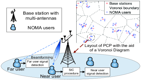
Figure 1: Illustration of the clustered NOMA networks with mmWave communications. The spatial distributions of the NOMA users follow the PCP.

In this paper, we focus on a typical pair of users from the typical cluster, where the paired User $k$ and User $j$ represent near user and far user, respectively. To analyze the performance of proposed networks, we introduce three user selection strategies for comparison which are as follows: 1) FNRF Scheme, where User $k$ is the $k$-th nearest receiver to the typical BS and User $j$ is randomly chosen from the rest farther NOMA users in the typical cluster; 2) RNFF Scheme, where User $j$ is the $j$-th nearest receiver to the typical BS and User $k$ is randomly chosen from the rest nearer NOMA users in the typical cluster; and 3) FNFF Scheme, where User $k$ and User $j$ are pre-decided and $1\leq k<j\leq 2K$.

II-B Blockage Effects

One remarkable characteristic of mmWave networks is that it is sensitive to be blocked by obstacles. Therefore, line-of-sight (LOS) links have a distinctive path loss law with non-line-of-sight (NLOS) transmissions. Note that each cluster can be visualized as a dense mmWave network due to the small variance $\sigma^{2}$ of NOMA users. Under this condition, one obstacle may block all receivers behind it, so we adopt the LOS disc to model the blockage effect [10, 41]. This blockage model fits the practical scenarios better than other patterns [18], especially for most urban scenarios with high buildings. Accordingly, the LOS probability inside the LOS disc with a radius $R_{L}$ is one, while the NLOS probability outside the disc is one. With the aid of such model, we provide the path loss law of our proposed networks with a distance $\dot{r}$ as follows

$$L_{p}(\dot{r})=\mathbf{U}\left({{R_{L}}-\dot{r}}\right){C_{L}}{\dot{r}^{-{\alpha_{L}}}}+\mathbf{U}\left({\dot{r}-{R_{L}}}\right){C_{N}}{\dot{r}^{-{\alpha_{N}}}},$$ (3)

where $C_{\kappa}$ is the intercept and $\alpha_{\kappa}$ is the path loss exponent. $\kappa=L$ and $N$ represent the LOS and NLOS links, respectively. $\mathbf{U}(.)$ is the unit step function.

II-C Uniform Linear Array

The channel model of mmWave is significantly different from the sub-6GHz networks due to the high free-space path loss. We adopt a popular model proposed in [42], where each BS employs the uniform linear array (ULA) antenna with $M$ elements. However, an omnidirectional antenna pattern is considered at NOMA users for simplifying the analysis. Hence the channel vector of mmWave signals from the BS to User $k$ can be expressed as

$${{\bf{h}}_{k}}=\sqrt{M}\sum\limits_{d=1}^{D}{{g_{kd}}}{\bf{a}}\left({{\theta_{kd}}}\right),$$ (4)

where ${{\bf{h}}_{k}}$ is a $M\times 1$ vector and $D$ is the number of multi-path. For $d$-th path, ${{g_{kd}}}$ is the complex small-scale fading gain and ${{\theta_{kd}}}$ is the spatial angle-of-departure (AoD). Due to the highly directional beamforming and quasi-optical property of mmWave signals. we assume $D=1$ in this paper, then the index $d$ can be dropped. For mmWave communications, $\left|{{g_{k}}}\right|$ follows independent Nakagami-$N_{\kappa}$ fading [10]. The ${{\bf{a}}\left(.\right)}$ is the transmit array response vector, which is expressed as follows:

$${\bf{a}}\left(\theta\right)=\frac{1}{{\sqrt{M}}}{\left[{1,...,{e^{j\pi m\theta}},...,{e^{j\pi\left({M-1}\right)\theta}}}\right]}^{T},$$ (5)

where $\theta=\frac{2q}{\lambda}\sin\varphi$ is uniformly distributed over $\left[{-\frac{2q}{\lambda},\frac{2q}{\lambda}}\right]$, and $m\in\left\{{0,...,M-1}\right\}$ is the antenna index. Here, $q$ denotes the spacing among antennas, $\lambda$ denotes the wavelength, and $\varphi$ denotes the physical AoD. In this paper, we consider $2q=\lambda$, namely a critically sampled environment.

II-D Analog Beamforming

Another constraint for mmWave networks is the high cost and power consumption for signal processing components. We adopt analog beamforming in this work for achieving a low complexity beamforming design. More particularly, the directions of beams are controlled by phase shifters. We invoke the optimal analog precoding which implies that the BSs try to align the direction of beams with the AoD of channels. Hence high beamforming gains can be obtained. In our system, we assume User $k$ is the primary user which requires higher quality of the service than User $j$. Therefore, the main beam direction of the typical BS is towards User $k$. The optimal analog vector for User $k$ can be expressed as

$${{\bf{w}}_{k}}={{\bf{a}}}\left({{\theta_{k}}}\right).$$ (6)

Then based on this precoding design, the effective channel gain at User $k$ aligning with the optimal analog beamforming is given by

$${\left|{{\bf{h}}_{k}^{H}{{\bf{w}}_{k}}}\right|^{2}}=M{\left|{{g_{k}}}\right|^{2}}{\left|{{{\bf{a}}^{H}}\left({{\theta_{k}}}\right){\bf{a}}\left({{\theta_{k}}}\right)}\right|^{2}}={M}{{{\left|{{g_{k}}}\right|}^{2}}}.$$ (7)

Regarding any other User $\hat{k}$, the effective channel gain is as follows

$${|{{\bf{h}}_{\hat{k}}^{H}{{\bf{w}}_{k}}}|^{2}}= \frac{{{{|{{g_{\hat{k}}}}|}^{2}}{{\left|{\sum\limits_{l=0}^{M-1}{{e^{-j\pi l\left({{\theta_{k}}-{\theta_{\hat{k}}}}\right)}}}}\right|}^{2}}}}{M}$$

$$= \frac{{{{\left|{{g_{\hat{k}}}}\right|}^{2}}{{\sin}^{2}}\left({\pi M\left({{\theta_{k}}-{\theta_{\hat{k}}}}\right)}/{2}\right)}}{{M{{\sin}^{2}}\left({\pi\left({{\theta_{k}}-{\theta_{\hat{k}}}}\right)}/2\right)}}$$

$$= M{\left|{{g_{\hat{k}}}}\right|^{2}}{G_{F}}\left({{\theta_{k}}-{\theta_{\hat{k}}}}\right),$$ (8)

where ${G_{F}}\left(\cdot\right)$ denotes the normalized Fejér kernel with parameter $M$. Note that $G_{F}(x)$ has a period of two. Therefore, $\left({{\theta_{k}}-{\theta_{\hat{k}}}}\right)$ is uniformly distributed over $[-1,1]$ [16].

II-E Signal Model

We assume that in the typical cluster, the typical BS is located at $y_{0}\in\Phi_{p}$. Then, User $k$ located at $x_{k}$ and User $j$ located at $x_{j}$ are paired and served by the same beam. The distances of them obey ${d_{k}}<{d_{j}}$. Moreover, the power allocation coefficients satisfy the conditions that $a_{k}<a_{j}$ and $a_{k}+a_{j}=1$, which is for fairness considerations [22]. In terms of other clusters, the interfering BS located at $y\in\Phi_{p}\backslash y_{0}$ provides an optimal analog beamforming for User $\xi_{y}$, which is chosen uniformly at random. As a consequence, the received signal is given by

$${y_{k}}= \underbrace{{\bf{h}}_{k}^{H}{{\bf{w}}_{k}}\sqrt{{a_{k}}{P_{t}}L_{p}\left({\left\|{{x_{k}}}\right\|}\right)}{s_{k}}}_{{\bf{Desired}}\;{\bf{Signal}}}+\underbrace{{\bf{h}}_{k}^{H}{{\bf{w}}_{k}}\sqrt{{a_{j}}{P_{t}}L_{p}\left({\left\|{{x_{k}}}\right\|}\right)}{s_{j}}}_{{\bf{SIC\ Signal}}}$$

$$+\underbrace{\sum\nolimits_{y\in\Phi_{p}\backslash{y_{0}}}{{\bf{h}}_{y\to k}^{H}{{\bf{w}}_{{\xi_{y}}}}\sqrt{{P_{t}}L_{p}\left({\left\|{{x_{k}}-y}\right\|}\right)}{s_{{\xi_{y}}}}}}_{{\bf{Inter}}-{\bf{Cluster}}}+\underbrace{{{\bf{n}}_{0}}}_{{\bf{Noise}}}$$ (9)

and

$${y_{j}}= \underbrace{{\bf{h}}_{j}^{H}{{\bf{w}}_{k}}\sqrt{{a_{j}}{P_{t}}L_{p}\left({\left\|{{x_{j}}}\right\|}\right)}{s_{j}}}_{{\bf{Desired}}\;{\bf{Signal}}}+\underbrace{{\bf{h}}_{j}^{H}{{\bf{w}}_{k}}\sqrt{{a_{k}}{P_{t}}L_{p}\left({\left\|{{x_{j}}}\right\|}\right)}{s_{k}}}_{{\bf{Intra}}-{\bf{Cluster}}\;}$$

$$+\underbrace{\sum\nolimits_{y\in\Phi_{p}\backslash{y_{0}}}{{\bf{h}}_{y\to j}^{H}{{\bf{w}}_{{\xi_{y}}}}\sqrt{{P_{t}}L_{p}\left({\left\|{{x_{j}}-y}\right\|}\right)}{s_{{\xi_{y}}}}}}_{{\bf{Inter}}-{\bf{Cluster}}}+\underbrace{{{\bf{n}}_{0}}}_{{\bf{Noise}}},$$ (10)

where ${\bf{h}}_{y\to\varpi}$ represents the channel vector from BS at $y$ to User $\varpi$ and $\varpi\in\{k,j\}$.

We assume that perfect SIC is carried out at User $k$, and hence User $k$ first decodes the signal of User $j$ with the following signal-to-interference-plus-noise-ratio (SINR)

$${\gamma_{k\to j}}=\frac{{{a_{j}}{{\left|{{\bf{h}}_{k}^{H}{{\bf{w}}_{k}}}\right|}^{2}}L_{p}\left({\left\|{{x_{k}}}\right\|}\right)}}{{{a_{k}}{{\left|{{\bf{h}}_{k}^{H}{{\bf{w}}_{k}}}\right|}^{2}}L_{p}\left({\left\|{{x_{k}}}\right\|}\right)+{I_{{\rm{inter}},k}}+\sigma_{n}^{2}}},$$ (11)

where ${I_{{\rm{inter}},\varpi}}=\sum\nolimits_{y\in\Phi_{p}\backslash{y_{0}}}{{|{{\bf{h}}_{y\to\varpi}^{H}{{\bf{w}}_{{\xi_{y}}}}}|^{2}}}L_{p}({\left\|{{x_{\varpi}}-y}\right\|})$. $\sigma_{n}^{2}$ is the noise power normalized by $P_{t}$.

If this decoding is successful, User $k$ then decodes the signal of itself. Based on (II-E), the SINR of User $k$ to decode its own message can be expressed as

$${\gamma_{k}}=\frac{{{a_{k}}{{\left|{{\bf{h}}_{k}^{H}{{\bf{w}}_{k}}}\right|}^{2}}L_{p}\left({\left\|{{x_{k}}}\right\|}\right)}}{{{I_{{\rm{inter}},k}}+\sigma_{n}^{2}}}.$$ (12)

Regarding User $j$, it directly decodes its own message by treating the signal of User $k$ as the interference. Based on (II-E), the SINR of User $j$ is given by

$${\gamma_{j}}=\frac{{{a_{j}}{{\left|{{\bf{h}}_{j}^{H}{{\bf{w}}_{k}}}\right|}^{2}}L_{p}\left({\left\|{{x_{j}}}\right\|}\right)}}{{{a_{k}}{{\left|{{\bf{h}}_{j}^{H}{{\bf{w}}_{k}}}\right|}^{2}}L_{p}\left({\left\|{{x_{j}}}\right\|}\right)+{I_{{\rm{inter}},j}}+\sigma_{n}^{2}}}.$$ (13)

III Distance Distributions

In this section, we discuss the distance distribution of NOMA users and BSs, which is the basis for analyzing the performance of our system. To simplify the notation, we first introduce a typical distribution named Rayleigh Distribution in the following part [13, 38].

Under Rayleigh Distribution, the PDF is given by

$${R_{p}}\left(v,\sigma\right)=\frac{v}{{{\sigma^{2}}}}\exp\left({-\frac{v^{2}}{{2{\sigma^{2}}}}}\right),v>0$$ (14)

and the cumulative distribution function (CDF) is as follows

$${R_{c}}\left({v,\sigma}\right)=1-\exp\left({-\frac{{{v^{2}}}}{{2{\sigma^{2}}}}}\right),v>0,$$ (15)

where $\sigma^{2}$ is the variance parameter as mentioned in (2).

III-A Distribution in FNRF Scheme

Under FNRF scheme, we start the analysis of intra-cluster distances from the typical BS to all NOMA users, and then inter-cluster distances from other BSs to the considered NOMA user.

III-A1 Distance Distribution of Near User

In the typical cluster, we assume that the distances between NOMA users and the typical BS form a set $\{R_{i}\}_{i=1:2K}$ which can be denoted by $\mathbb{R}_{y_{0}}$. The realization of $R_{i}$ is defined as ${r_{i}}=\left\|{x_{i}}\right\|$, where $x_{i}\in\mathbb{N}_{y_{0}}$. Note that $x_{i}$ is i.i.d. as a Gaussian random variable with $\sigma^{2}$. If the considered NOMA user is selected at random, we are able to drop the index $i$ from $r_{i}$ since every $r_{i}$ follows the same distribution. Under this condition, $r$ is a Gaussian random variable with variance $\sigma^{2}$, so the PDF of distance $r$ is as follows [13]

$$f_{r}\left(r\right)={R_{p}}\left(v,\sigma\right).$$ (16)

Compared with the aforementioned randomly choosing case, we are more interested in the ordered distance distribution due to the fact that User $k$ is always closer to the typical BS than User $j$. Accordingly, we assume that $i$ is the distance rank parameter. In other words, the first nearest NOMA user is located at $x_{1}$, the second nearest one is located at $x_{2}$, and so forth. Assuming the $i$-th closest NOMA user at $x_{i}$ has a distance $r_{i}$ to the typical BS, with the aid of the $i$-th order statistic in [43], the PDF of distance $r_{i}$ in the typical cluster is given by

$$f_{d}^{i}\left({{r_{i}}}\right)= \frac{{\left({2K}\right)!}}{{\left({i-1}\right)!\left({2K-i}\right)!}}\frac{{{r_{i}}}}{{{\sigma^{2}}}}\sum\limits_{w=0}^{i-1}{{{\left({-1}\right)}^{i-1-w}}{{i-1}\choose w}}$$

$$\times{\exp\left({-\frac{{\left({2K-w}\right)r_{i}^{2}}}{{2{\sigma^{2}}}}}\right)}.$$ (17)

Based on the discussion in (III-A1), it is effortless to derive the PDF of near user distance under the FNRF strategy.

Corollary 1.

Note that near user in the FNRF scheme is the $k$-th nearest NOMA user at $x_{k}$ and $1\leq k\leq 2K-1$. The distribution of the distance $r_{k}=\|x_{k}\|$ from near user to the typical BS is as follows

$$f_{\rm FR}^{k}\left({{r_{k}}}\right)=f_{d}^{k}(r_{k}).$$ (18)

Proof:

We substitute $i=k$ into (III-A1) to obtain (18). ∎

III-A2 Distance Distribution of Far User

In contrast to near user, far user in the FNRF scheme is randomly chosen from the rest farther NOMA users in the typical cluster. Assuming the possible User $j$ is located at $x_{j}\in\mathbb{N}_{y_{0}}/x_{1},x_{2},...,x_{k}$ with a distance $r_{j}=\left\|{x_{j}}\right\|$, the distribution of distance $r_{j}$ is expressed in the following lemma.

Lemma 1.

The randomly selected far user in the FNRF scheme at $x_{j}$ has a distance $r_{j}$ to the typical BS and $r_{j}>r_{k}$, so the conditional PDF of distance $r_{k}$ is given by

$$f_{\rm FR}^{j}\left({{r_{j}}}{|{r_{k}}}\right)=\left\{{\begin{array}[]{*{20}{c}}{\frac{{{R_{p}}\left({{r_{j}},\sigma}\right)}}{{1-{R_{c}}\left({{r_{k}},\sigma}\right)}}},&{{r_{j}}>{r_{k}}}\\ 0,&{{r_{j}}\leq{r_{k}}}\\ \end{array}}\right..$$ (21)

Proof:

When ${{r_{j}}\leq{r_{k}}}$, the probability is zero as far user is defined to be located farther than near user with a distance $r_{k}$. Under the other condition $r_{j}>r_{k}$, the possible User $j$ follows Rayleigh distribution over the rang $(r_{k},\infty]$. Therefore, such distance distribution can be summarized in Lemma 1. ∎

III-A3 Distance Distribution of Interfering BSs

The distance distribution of interfering BSs can be deduced from probability generating functional of PPP [44]. The detailed deriving procedure is provided in the next section.

Remark 1.

Since the typical pair of users are located in the typical cluster, the distance distribution of interfering BSs is same for all considered user selection strategies and thus we omit the analysis of such distribution in the other scheme.

III-B Distribution in RNFF Scheme

Under the RNFF scheme, we focus on the distribution of intra-cluster distances. Both near user and far user have different distributions with those in the FNRF scheme. We first analyze the far user and then the near user.

III-B1 Distance Distribution of Far User

The location of considered far user is assumed to be $x_{j}$ with a distance $r_{j}$. Since far user becomes the $j$-th nearest intra-cluster NOMA user, the distribution of distance $r_{j}$ can be expressed in the following part.

Lemma 2.

The considered far user under RNFF scheme is the $j$-th closest NOMA receiver located at $x_{j}$ with a distance $r_{j}$ and $2\leq j\leq 2K$. Therefore the PDF of distance $r_{j}$ is given by

$$f_{\rm RF}^{j}\left({{r_{j}}}\right)=f_{d}^{j}(r_{j}).$$ (22)

Proof:

The proof procedure is similar to Corollary 1, but with the different condition that $i=j$. ∎

III-B2 Distance Distribution of near User

Near user under the RNFF scheme is randomly selected from the remaining closer NOMA users in the typical cluster. We assume the considered near user is located at $x_{k}$ with a distance $r_{k}=||x_{k}||$. Under this condition, the distance distribution of such near user can be calculated in the following lemma.

Lemma 3.

The randomly chosen User $k$ under RNFF scheme at $x_{k}$ has a distance $r_{k}$ to the typical BS, so the PDF of distance $r_{k}$ is expressed as follows

$$f_{\rm RF}^{j}\left({{r_{k}}|{r_{j}}}\right)=\left\{{\begin{array}[]{*{20}{c}}{\frac{{{R_{p}}\left({{r_{k}},\sigma}\right)}}{{{R_{c}}\left({{r_{j}},\sigma}\right)}},}&{{r_{k}}<{r_{j}}}\\ {0,}&{{r_{k}}\geq{r_{j}}}\\ \end{array}}\right..$$ (25)

Proof:

The proof is similar to Lemma 1 and thus we skip it here. ∎

III-C Distribution in FNFF Scheme

Since the near user and far user are pre-decided in the FNFF scheme, the distance distributions of User $k$ and User $j$ are same with Corollary 1 and Lemma 2, respectively. Therefore, the PDF of two corresponding distributions are as follows: $f_{\rm FF}^{k}(r_{k})=f_{d}^{k}(r_{k})$ and $f_{\rm FF}^{j}(r_{j})=f_{d}^{j}(r_{j})$.

IV Performance Evaluation

In this section, we characterize the coverage performance and system throughput of three different user selection strategies depending on the distributions of intra/inter-cluster distances.

IV-A FNRF Scheme

The FNRF scheme is suitable for the condition that the primary user (User $k$) is pre-decided. To enhance the generality, User $k$ can be any user in the typical cluster. On the other side, far user (User $j$) is selected at random from the rest farther NOMA users to provide a fair selection law. All possible far users have the equal opportunity to be the paired one. Moreover, such random selection strategy do not require the instantaneous CSI of User $j$. To make the tractable analysis, we first deduce the Laplace Transform of Interferences in the following part.

IV-A1 Laplace Transform of Interferences

We only concentrate on the Laplace transform of inter-cluster interferences because there is no interfering device located in the typical cluster. Moreover, the expression is suitable for all user selection strategies due to the fact mentioned in Remark 1.

Lemma 4.

The inter-cluster interferences are provided from all BSs except the typical BS, then a closed-form approximation for the Laplace transform of such interferences is given by

$${\mathcal{L}_{I}}(s)\simeq\exp\left({-\frac{{{\pi^{2}}{\lambda_{c}}R_{L}^{2}}}{{{n_{1}}}}\sum\limits_{{i_{1}}=1}^{{n_{1}}}{\mathcal{G}_{F}^{I}\bigg{(}s,{\frac{{{\zeta_{{i_{1}}}+1}}}{2}}\bigg{)}\sqrt{1-\zeta_{{i_{1}}}^{2}}}}\right),$$ (26)

where

$$\mathcal{G}_{F}^{I}\left(s,g\right)= {\rho_{N}}\left({\frac{{sM{C_{N}}{G_{F}}\left(g\right)}}{{{N_{N}}R_{L}^{{\alpha_{N}}}}}}\right)-{\rho_{L}}\left({\frac{{{N_{L}}R_{L}^{{\alpha_{L}}}}}{{sM{G_{F}}\left(g\right){C_{L}}}}}\right),$$ (27)

$${\rho_{L}}\left(v\right)= {}_{2}{F_{1}}\left({{N_{L}},{N_{L}}+\frac{2}{{{\alpha_{L}}}};{N_{L}}+\frac{2}{{{\alpha_{L}}}}+1;-v}\right)$$

$$\times\frac{{{2v^{{N_{L}}}}}}{{\left({{\alpha_{L}}{N_{L}}+2}\right)}},$$ (28)

$${\rho_{N}}\left(v\right)= {}_{2}{F_{1}}\left({-\frac{2}{{{\alpha_{N}}}},{N_{N}};1-\frac{2}{{{\alpha_{N}}}};-v}\right),(\alpha_{N}>2),$$ (29)

${}_{2}F_{1}(.)$ is Gauss hypergeometric function. ${\zeta_{{i_{1}}}}=\cos\left({\frac{{2{i_{1}}-1}}{{2{n_{1}}}}\pi}\right)$ over $[-1,1]$ denotes the Gauss-Chebyshev node and $i_{1}=1,2,...,n_{1}$. The parameter $n_{1}$ has a function to balance the complexity and accuracy [29]. Only if the $n_{1}\rightarrow\infty$, the equality is established.

Proof:

See Appendix A. ∎

For most mmWave carrier frequencies, the path loss exponent of LOS communications equals two, namely $\alpha_{L}=2$, which has been proved by several actual channel measures [45, 46, 47]. In terms of the NLOS interferences, numerous papers [10, 48] have indicated that NLOS signals are weak enough to be ignored in mmWave communications. Therefore, we propose the first special case blew to simplify the calculation.

Special Case 1: When deriving the Laplace transform of interference, we ignore all NLOS interferences due to the negligible impact on the final performance and $\alpha_{L}$ is assumed to be $2$.

Lemma 5.

Under special case 1, the tight approximation for Laplace transform of inter-cluster interferences in Lemma 4 can be simplified as follows

$${{\tilde{\mathcal{L}}}_{I}}\left(s\right)\simeq\exp\left({-\frac{{{\pi^{2}}{\lambda_{c}}R_{L}^{2}}}{{{n_{1}}}}\sum\limits_{{i_{1}}=1}^{{n_{1}}}{\tilde{\mathcal{G}}_{I}^{F}\left({\frac{{{\zeta_{{i_{1}}}+1}}}{2}}\right)\sqrt{1-\zeta_{{i_{1}}}^{2}}}}\right),$$ (30)

where

$$\tilde{\mathcal{G}}_{I}^{F}\left({s,g}\right)=1+{F_{{\alpha_{L}}}}\left({\frac{{sM{G_{F}}\left(g\right){C_{L}}}}{{{N_{L}}R_{L}^{2}}}}\right),$$ (31)

$${F_{{\alpha_{L}}}}\left(v\right)=-\frac{1}{{{{\left({1+v}\right)}^{{N_{L}}-1}}}}-{N_{L}}v$$

$$\times\left({\sum\limits_{{m_{L}}=1}^{{N_{L}}-1}{\frac{1}{{{{\left({1+v}\right)}^{{N_{L}}-{m_{L}}}}\left({{N_{L}}-{m_{L}}}\right)}}}-\ln\left({1+\frac{1}{v}}\right)}\right).$$ (32)

Proof:

As NLOS interferences are ignored, ${\rho_{N}}\left(v\right)$ should be removed from Lemma 4. Moreover, when $\alpha_{L}=2$, ${\rho_{L}}\left(v\right)$ can be simplified by using the similar method as discussed in the Appendix A of [49]. Lastly, utilizing the similar proof method as Lemma 4, the simpler equation than (26) can be expressed in (30). ∎

IV-A2 Coverage Probability for Near User

We introduce two SINR thresholds $\tau_{k}$ and $\tau_{j}$ for User $k$ and User $j$, respectively. These thresholds should satisfy the condition $({a_{j}}-{\tau_{j}}{a_{k}}>0)$ to ensure the success of NOMA protocols [29]. Since near user has the SIC procedure, the decoding for User $k$ will be success only when $({\gamma_{k\to j}}>\tau_{j})$. If this condition is satisfied, the coverage probability for near user is the percentage of the received SINR $\gamma_{k}$ that excess $\tau_{k}$. Therefore, the coverage probability for User $k$ under the FNRF scheme can be defined as follows

$$P_{k}^{{\rm FR}}\left({{\tau_{k}},{\tau_{j}}}\right)=\mathbb{P}\left[{{\gamma_{k}}>{\tau_{k}},{\gamma_{k\to j}}>{\tau_{j}}}\right].$$ (33)

With the aid of Laplace transform of interferences as discussed in Lemma 4, the expression for coverage probability is shown in the following theorem.

Theorem 1.

With different value of thresholds $\tau_{k}$ and $\tau_{j}$, the coverage probability for User $k$ can be divided into two cases. Firstly, for Range 1 $R_{1}$: ${a_{k}}{\tau_{j}}<{a_{j}}\leq{a_{k}}{\tau_{j}}\left({1+\frac{1}{{{\tau_{k}}}}}\right)$, the expression under the FNRF scheme is given by

$$P_{k}^{\rm FR}\left({{\tau_{k}},{\tau_{j}}}\right)\approx \int_{0}^{{R_{L}}}{{\Theta_{L}}\left({{r_{k}},{\tau_{j}},{a_{j}}-{\tau_{j}}{a_{k}}}\right)f_{\rm FR}^{k}\left({{r_{k}}}\right)d{r_{k}}}$$

$$+\int_{{R_{L}}}^{\infty}{{\Theta_{N}}\left({{r_{k}},{\tau_{j}},{a_{j}}-{\tau_{j}}{a_{k}}}\right)f_{\rm FR}^{k}\left({{r_{k}}}\right)d{r_{k}}},$$ (34)

where

$${\Theta_{\kappa}}\left({r,\tau,\beta}\right)= {\sum\limits_{{n_{\kappa}}=1}^{{N_{\kappa}}}{\left({-1}\right)}^{{n_{\kappa}}+1}}{N_{\kappa}\choose n_{\kappa}}\exp\left({-\frac{{{n_{\kappa}}{\psi_{\kappa}}\tau{r^{{\alpha_{\kappa}}}}\sigma_{n}^{2}}}{{\beta M{C_{\kappa}}}}}\right)$$

$$\times{\mathcal{L}_{I}}\left({\frac{{{n_{\kappa}}{\psi_{\kappa}}\tau{r^{{\alpha_{\kappa}}}}}}{{\beta M{C_{\kappa}}}}}\right),$$ (35)

and ${\psi_{\kappa}}={N_{\kappa}}{\left({{N_{\kappa}}!}\right)^{-1/{N_{\kappa}}}}$.

On the other hand, for Range 2 $R_{2}$: ${a_{j}}>{a_{k}}{\tau_{j}}\left({1+\frac{1}{{{\tau_{k}}}}}\right)$, the coverage probability is changed to

$$P_{k}^{\rm FR}\left({{\tau_{k}},{\tau_{j}}}\right)\approx \int_{0}^{{R_{L}}}{{\Theta_{L}}\left({{r_{k}},{\tau_{k}},{a_{k}}}\right)f_{\rm FR}^{k}\left({{r_{k}}}\right)d{r_{k}}}$$

$$+\int_{{R_{L}}}^{\infty}{{\Theta_{N}}\left({{r_{k}},{\tau_{k}},{a_{k}}}\right)f_{\rm FR}^{k}\left({{r_{k}}}\right)d{r_{k}}}.$$ (36)

Proof:

See Appendix B. ∎

Remark 2.

It is obvious that if the realistic scenario fits the condition ${a_{j}}={a_{k}}{\tau_{j}}\left({1+\frac{1}{{{\tau_{k}}}}}\right)$, the coverage probability for $R_{1}$ and $R_{2}$ will share the same expression.

Corollary 2.

Under special case 1, a simpler expression than Theorem 1 is given by

$$\tilde{P}_{k}^{\rm FR}\left({{\tau_{k}},{\tau_{j}}}\right)=P_{k}^{\rm FR}\left({{\tau_{k}},{\tau_{j}}}\right)\left|{{}_{{\mathcal{L}_{I}}\left(.\right)\to{\mathcal{\tilde{L}}_{I}}\left(.\right)}}\right.,$$ (37)

where ${{\mathcal{L}_{I}}(.)\to{\mathcal{\tilde{L}}_{I}}(.)}$ means using ${\mathcal{\tilde{L}}_{I}}(.)$ to replace ${\mathcal{L}_{I}}(.)$.

Proof:

With the aid of Lemma 5 and Theorem 1, we obtain (37). ∎

In the reality, the coverage radius of the macro BS is always larger than $R_{L}$, which means the majority of BSs communicate with the considered user via NLOS links. Note that the received power from NLOS signals is negligible. We propose the second special case.

Special Case 2: In a sparse network, the density of BSs is small enough to ensure that the majority of BSs utilize NLOS links to provide the inter-cluster interferences. Together with the fact that the impact of NLOS signals is tiny, we ignore all inter-cluster interferences and the coverage probability from NLOS links, namely, ${\mathcal{L}_{I}}(.)=1$ and $\Theta_{N}(.)=0$. Moreover, we keep assuming $\alpha_{L}=2$ as discussed in special case 1.

Remark 3.

As NOMA users are randomly distributed in the typical cluster, each of them has an opportunity to communicate with the typical BS through an NLOS link. To ensure the considered number of intra-cluster users is fixed as $2K$, we should take every LOS and NLOS NOMA receivers into account when calculating the coverage. Therefore $\Theta_{N}(.)=0$ does not indicate that we only consider NOMA receivers with LOS links. It actually means the received SINR at all NOMA users with NLOS links fails to surpass the required threshold.

Corollary 3.

Under special case 2, the closed-form coverage probability for near user is at the top of next page.

$$\hat{P}_{k}^{\rm FR}\left({{\tau_{k}},{\tau_{j}}}\right)\approx\left\{{\begin{array}[]{*{20}{c}}{\frac{\Gamma_{k}}{{{\sigma^{2}}}}{{\sum\limits_{{n_{L}}=1}^{{N_{L}}}}{\sum\limits_{{w}=0}^{{k-1}}}{\left({-1}\right)}^{{n_{L}+k-w}}}{{k-1}\choose w}{N_{L}\choose n_{L}}\frac{{1-\exp\left({-A_{1}\left({{\tau_{j}}}\right)R_{L}^{2}}\right)}}{{A_{1}\left({{\tau_{j}}}\right)}},}&{R_{1}}\\ {\frac{\Gamma_{k}}{{{\sigma^{2}}}}{{\sum\limits_{{n_{L}}=1}^{{N_{L}}}}{\sum\limits_{{w}=0}^{{k-1}}}{\left({-1}\right)}^{{n_{L}+k-w}}}{{k-1}\choose w}{N_{L}\choose n_{L}}\frac{{1-\exp\left({-A_{2}\left({{\tau_{k}}}\right)R_{L}^{2}}\right)}}{{A_{2}\left({{\tau_{k}}}\right)}},}&{R_{2},}\end{array}}\right.$$ (40)

In (40), $\Gamma_{k}=\frac{(2K)!}{2(k-1)!(2K-k)!}$, ${A_{1}}\left({{\tau_{j}}}\right)=\frac{{{n_{L}}{\psi_{L}}{\tau_{j}}\sigma_{n}^{2}}}{{\left({{a_{j}}-{\tau_{j}}{a_{k}}}\right)M{C_{L}}}}+\frac{(2K-w)}{{{2\sigma^{2}}}}$, and ${A_{2}}\left({{\tau_{k}}}\right)=\frac{{{n_{L}}{\psi_{L}}{\tau_{k}}\sigma_{n}^{2}}}{{{a_{k}}M{C_{L}}}}+\frac{(2K-w)}{{{2\sigma^{2}}}}$.

Proof:

By substituting ${\mathcal{L}_{I}}(.)=1$ and $\Theta_{N}(.)=0$ into Theorem 1, we obtain the equation for $R_{1}$ as follows

$$\hat{P}_{k}^{\rm FR}\left({{\tau_{k}},{\tau_{j}}}\right)\approx \int_{0}^{{R_{L}}}{{{\sum\limits_{{n_{L}}=1}^{{N_{L}}}{\left({-1}\right)^{{n_{L}}+1}}}}}{N_{L}\choose n_{L}}$$

$$\times\exp\left({-\frac{{{n_{L}}{\psi_{L}}{\tau_{j}}r_{k}^{2}\sigma_{n}^{2}}}{{\left({{a_{j}}-{\tau_{j}}{a_{k}}}\right)M{C_{L}}}}}\right)f_{\rm FR}^{k}\left({{r_{k}}}\right)dr_{k}.$$ (41)

With the fact $\int_{0}^{B}{v\exp\left({-A{v^{2}}}\right)dv}=\frac{{1-\exp\left({-A{B^{2}}}\right)}}{{2A}}$, (3) can be simplified into the expression in (40) under $R_{1}$. Utilizing the same method, we are able to derive the closed-form expression for $R_{2}$. Then the proof is complete. ∎

Remark 4.

The coverage probability for all users under special case 2 is independent with $\lambda_{c}$ since such density is only contained in $\mathcal{L}_{I}(.)$.

Remark 5.

With the aid of Corollary 3, we are able to conclude that the coverage probability for near user is a monotonic increasing function with $M$, while it has a negative correlation with $\sigma_{n}^{2}$ and its corresponding threshold. Moreover, for $R_{1}$, $\hat{P}_{k}^{\rm FR}(.)$ has a positive correlation with $({a_{j}}-{\tau_{j}}{a_{k}})$ and for $R_{2}$, $\hat{P}_{k}^{\rm FR}(.)$ increases with the rise of $a_{k}$. These insights can be figured out from (3), which can be rewritten as follows:

$$\hat{P}_{k}^{{\rm{FR}}}\left({{\tau_{k}},{\tau_{j}}}\right)\approx \int_{0}^{{R_{L}}}{\left({1-{{\left({1-\exp\left({-\frac{{{\psi_{L}}{\tau_{j}}r_{k}^{2}\sigma_{n}^{2}}}{{\varrho M{C_{L}}}}}\right)}\right)}^{{N_{L}}}}}\right)}$$

$$\times f_{{\rm{FR}}}^{k}\left({{r_{k}}}\right)d{r_{k}},$$ (42)

where for the range $R_{1}$, $\varrho=({a_{j}}-{\tau_{j}}{a_{k}})$, while for the range $R_{2}$, $\varrho=a_{k}$.

IV-A3 Coverage Probability for Far User

In contrast to the near user, the coverage probability for User $j$ at $x_{j}$ only depends on $\tau_{j}$. However, as the directional beamforming of the typical BS is aligned towards User $k$, the effective channel gain for User $j$ fits (II-D) rather than (7). Note that far user is randomly selected from the farther intra-cluster NOMA receivers. We define the coverage probability for far user as follows

$$P_{j}^{\rm RF}\left({{\tau_{j}}}\right)=\mathbb{P}\left[{{\gamma_{j}}>{\tau_{j}}}\right].$$ (43)

As discussed in Lemma 2 and Laplace transform of interferences, we obtain the coverage probability expression for User $j$ in the following theorem.

Theorem 2.

Under the FNRF scheme, the coverage probability for User $j$ at $x_{j}$ with a distance $r_{j}$ is given by

$$P_{j}^{\rm FR}\left({{\tau_{j}}}\right)\approx\frac{\pi}{{{n_{2}}}}\sum\limits_{{i_{2}}=1}^{{n_{2}}}{\mathcal{G}_{j}^{\rm RF}\left({{\tau_{j}},\frac{{{\zeta_{{i_{2}}}+1}}}{2}}\right)}\sqrt{1-\zeta_{{i_{2}}}^{2}},$$ (44)

where

$$\mathcal{G}_{j}^{\rm FR}\left({{\tau_{j}},g}\right)\approx \int_{0}^{{R_{L}}}{\int_{{r_{k}}}^{{R_{L}}}{{\Theta_{L}}\left({{r_{j}},{\tau_{j}},\left({{a_{j}}-{\tau_{j}}{a_{k}}}\right){G_{F}}\left(g\right)}\right)}}$$

$$\times{f_{\rm FR}^{j}\left({{r_{j}}}|r_{k}\right)d{r_{j}}}f_{\rm FR}^{k}\left({{r_{k}}}\right)dr_{k}$$

$$+\int_{{R_{L}}}^{\infty}{\int_{{r_{k}}}^{\infty}{{\Theta_{N}}\left({{r_{j}},{\tau_{j}},\left({{a_{j}}-{\tau_{j}}{a_{k}}}\right){G_{F}}\left(g\right)}\right)}}$$

$$\times{f_{\rm FR}^{j}\left({{r_{j}}}|r_{k}\right)d{r_{j}}}f_{\rm FR}^{k}\left({{r_{k}}}\right)dr_{k}.$$ (45)

Proof:

See Appendix C. ∎

Corollary 4.

Under special case 1, the simpler expression than Theorem 2 is shown as follows

$$\tilde{P}_{j}^{\rm FR}\left({{\tau_{j}}}\right)=P_{j}^{\rm FR}\left({{\tau_{j}}}\right)\left|{{}_{{{\cal L}_{I}}\left(.\right)\to{{\tilde{\cal L}}_{I}}\left(.\right)}}\right..$$ (46)

Proof:

The proof procedure is similar to Corollary 2 and thus we omit it here. ∎

Corollary 5.

Under special case 2, in a sparse network, the closed-form coverage probability for far user is given by

$$\hat{P}_{j}^{\rm FR}\left({{\tau_{j}}}\right)\approx\frac{\pi}{{{n_{2}}}}\sum\limits_{{i_{2}}=1}^{{n_{2}}}{\hat{\mathcal{G}}_{j}^{\rm FR}\left({{\tau_{j}},\frac{{{\zeta_{{i_{2}}}+1}}}{2}}\right)}\sqrt{1-\zeta_{{i_{2}}}^{2}},$$ (47)

where

$$\hat{\mathcal{G}}_{j}^{\rm FR}\left({{\tau_{j}},g}\right)=\sum\limits_{{n_{L}}=1}^{{N_{L}}}{{{\left({-1}\right)}^{{n_{L}}+1}}}{N_{L}\choose n_{L}}\frac{K}{{2{\sigma^{4}}Q\left({{\tau_{j}},g}\right)}}$$

$$\times\bigg{(}{\frac{1}{{Q\left({{\tau_{j}},g}\right)+\chi}}+\frac{{Q\left({{\tau_{j}},g}\right)\exp\left({-\left({Q\left({{\tau_{j}},g}\right)+\chi}\right)R_{L}^{2}}\right)}}{{\left({Q\left({{\tau_{j}},g}\right)+\chi}\right)\chi}}}$$

$${-\exp\left({-Q\left({{\tau_{j}},g}\right)R_{L}^{2}}\right)}\bigg{)},$$ (48)

and $Q\left({{\tau_{j}},g}\right)=\frac{{{n_{L}}{\psi_{L}}{\tau_{j}}\sigma_{n}^{2}}}{{\left({{a_{j}}-{\tau_{j}}{a_{k}}}\right){G_{F}}\left(g\right)M{C_{L}}}}+\frac{1}{{2{\sigma^{2}}}}$ and $\chi=\frac{{2K-1}}{{2{\sigma^{2}}}}$.

Proof:

With the similar proof as discussed in Corollary 3, we obtain Corollary 5. ∎

Remark 6.

The coverage probability for far user has the same features with near user as mentioned in Remark 5. The only difference is the relationship to $M$. Corollary 5 demonstrates that the value of ${\hat{\mathcal{G}}_{j}^{\rm FR}\left({{\tau_{j}},g}\right)}$ is decided by $G_{F}(g)M$ which is fluctuant with the increase of $M$. Such monotonic increasing relation with $M$ for near user will not exist in the far user scenario.

IV-B RNFF Scheme

Comparing with the FNRF scheme, the RNFF strategy focuses on a certain far user which requires continuous services. In this scheme, User $j$ is the $j$-th nearest user to the typical BS and User $k$ is randomly selected from the rest closer intra-cluster NOMA receivers.

IV-B1 Coverage Probability for Near User

Under the RNFF scheme, the coverage probability for User $k$ with the thresholds $\tau_{k}$ and $\tau_{j}$ is defined as follows.

$$P_{k}^{\rm RF}\left({{\tau_{k}},{\tau_{j}}}\right)=\mathbb{P}\left[{{\gamma_{k}}>{\tau_{k}},{\gamma_{k\to j}}>{\tau_{j}}}\right].$$ (49)

As the distance distribution of near user is dependent on the distance of far user $r_{j}$, the coverage probability can be expressed in the following part.

Theorem 3.

Same with FNRF scheme, the coverage probability of near user in the RNFF scheme can be divided into two ranges $R_{1}$ and $R_{2}$ and it is given at the top of next page.

$$P_{k}^{\rm RF}\left({{\tau_{k}},{\tau_{j}}}\right)\approx\left\{{\begin{array}[]{*{20}{c}}\begin{array}[]{l}\int_{0}^{{R_{L}}}{\int_{0}^{{r_{j}}}{{\Theta_{L}}\left({{r_{k}},{\tau_{j}},{a_{j}}-{\tau_{j}}{a_{k}}}\right)}f_{\rm RF}^{k}\left({{r_{k}}|{r_{j}}}\right)dr_{k}f_{\rm RF}^{j}\left({{r_{j}}}\right)d{r_{j}}}\\ +\int_{{R_{L}}}^{\infty}{\int_{{R_{L}}}^{{r_{j}}}{{\Theta_{N}}\left({{r_{k}},{\tau_{j}},{a_{j}}-{\tau_{j}}{a_{k}}}\right)}f_{\rm RF}^{k}\left({{r_{k}}|{r_{j}}}\right)dr_{k}f_{\rm RF}^{j}\left({{r_{j}}}\right)d{r_{j}}},\\ \end{array}&{R{{}_{1}}}\\ \begin{array}[]{l}\int_{0}^{{R_{L}}}{\int_{0}^{{r_{j}}}{{\Theta_{L}}\left({{r_{k}},{\tau_{k}},{a_{k}}}\right)}f_{\rm RF}^{k}\left({{r_{k}}|{r_{j}}}\right)dr_{k}f_{\rm RF}^{j}\left({{r_{j}}}\right)d{r_{j}}}\\ +\int_{{R_{L}}}^{\infty}{\int_{{R_{L}}}^{{r_{j}}}{{\Theta_{N}}\left({{r_{k}},{\tau_{k}},{a_{k}}}\right)}f_{\rm RF}^{k}\left({{r_{k}}|{r_{j}}}\right)dr_{k}f_{\rm RF}^{j}\left({{r_{j}}}\right)d{r_{j}}},\\ \end{array}&{R{{}_{2}}.}\\ \end{array}}\right.$$ (56)

Proof:

Note that the distance distribution of near user shown in Lemma 3 is depended on the distance $r_{j}$. With the similar proof procedure in Theorem 1, we obtain (56). ∎

Corollary 6.

Under special case 1, we obtain the simpler equation of coverage probability for near user as follows

$$\tilde{P}_{k}^{\rm RF}\left({{\tau_{k}},{\tau_{j}}}\right)=P_{k}^{\rm RF}\left({{\tau_{k}},{\tau_{j}}}\right)\left|{{}_{{{\cal L}_{I}}\left(.\right)\to{{\tilde{\cal L}}_{I}}\left(.\right)}}\right..$$ (57)

Proof:

With the same reason in Corollary 2, we provide the simpler expression for coverage probability in (57). ∎

Corollary 7.

Under special case 2, the closed-form expression of coverage probability for near user in the FNRF scheme is given by

$$\hat{P}_{k}^{\rm RF}\left({{\tau_{k}},{\tau_{j}}}\right)\approx$$

$$\left\{{\begin{array}[]{*{20}{c}}{\sum\limits_{{n_{L}}=1}^{{N_{L}}}{\sum\limits_{w=0}^{k-1}{{{\left({-1}\right)}^{{n_{L}}+k-w}}{k-1\choose w}}{N_{L}\choose n_{L}}}\frac{\Gamma_{k}}{{{\sigma^{2}}{A_{3}}\left({{\tau_{j}}}\right)}}}\\ \times{\left({\Omega\left({\frac{{\left({2K-w}\right)}}{{2{\sigma^{2}}}}+{A_{3}}\left({{\tau_{j}}}\right)}\right)-\Omega\left({\frac{{\left({2K-w}\right)}}{{2{\sigma^{2}}}}}\right)}\right),}&{R_{1}}\\ {\sum\limits_{{n_{L}}=1}^{{N_{L}}}{\sum\limits_{w=0}^{k-1}{{{\left({-1}\right)}^{{n_{L}}+k-w}}{k-1\choose w}}{N_{L}\choose n_{L}}}\frac{\Gamma_{k}}{{{\sigma^{2}}{A_{4}}\left({{\tau_{k}}}\right)}}}\\ \times{\left({\Omega\left({\frac{{\left({2K-w}\right)}}{{2{\sigma^{2}}}}+{A_{4}}\left({{\tau_{k}}}\right)}\right)-\Omega\left({\frac{{\left({2K-w}\right)}}{{2{\sigma^{2}}}}}\right)}\right),}&{R_{2}}\\ \end{array}}\right.$$ (62)

where $\Omega\left(\delta\right)=\varphi\left({2{\sigma^{2}}\delta}\right)+\frac{{\exp\left({-\delta R_{L}^{2}}\right)}}{{2{\sigma^{2}}\delta}}$, ${A_{3}}\left({{\tau_{j}}}\right)=\frac{{{n_{L}}{\psi_{L}}{\tau_{j}}\sigma_{n}^{2}}}{{\left({{a_{j}}-{\tau_{j}}{a_{k}}}\right)M{C_{L}}}}+\frac{1}{{2{\sigma^{2}}}}$, ${A_{4}}\left({{\tau_{k}}}\right)=\frac{{{n_{L}}{\psi_{L}}{\tau_{k}}\sigma_{n}^{2}}}{{{a_{k}}M{C_{L}}}}+\frac{1}{{2{\sigma^{2}}}}$ and $\varphi(.)$ is the Psi function [50].

Proof:

See Appendix D. ∎

Remark 7.

When $K=1$, Corollary 7 equals to Corollary 3. In other words, the coverage probabilities for near user in the FNRF and RNFF schemes are same under the condition $K=1$.

Remark 8.

The properties for the near user in the RNFF scheme are same with those in the FNRF scheme as discussed in Remark 5.

IV-B2 Coverage Probability for Far User

In terms of the far user in RNFF scheme, as it is the $j$-th nearest NOMA transmitter in the typical cluster, the coverage probability can be defined as follows.

$$P_{j}^{\rm RF}\left({{\tau_{j}}}\right)=\mathbb{P}\left[{{\gamma_{j}}>{\tau_{j}}}\right].$$ (63)

Theorem 4.

Under the RNFF scheme, the coverage probability of far user can be expressed as

$$P_{j}^{\rm RF}\left({{\tau_{j}}}\right)\approx\frac{\pi}{{{n_{2}}}}\sum_{{i_{2}}=1}^{{n_{2}}}\mathcal{G}_{j}^{\rm RF}\left({{\tau_{j}},\frac{{{\zeta_{{i_{2}}}+1}}}{2}}\right)\sqrt{1-\zeta_{{i_{2}}}^{2}},$$ (64)

where

$$\mathcal{G}_{j}^{\rm RF}\left({{\tau_{j}},g}\right)$$

$$\approx \int_{0}^{{R_{L}}}{{\Theta_{L}}\left({{r_{j}},{\tau_{j}},\left({{a_{j}}-{\tau_{j}}{a_{k}}}\right){G_{F}}\left(g\right)}\right)f_{\rm RF}^{j}\left({{r_{j}}}\right)d{r_{j}}}$$

$$+\int_{0}^{{R_{L}}}{{\Theta_{N}}\left({{r_{j}},{\tau_{j}},\left({{a_{j}}-{\tau_{j}}{a_{k}}}\right){G_{F}}\left(g\right)}\right)f_{\rm RF}^{j}\left({{r_{j}}}\right)d{r_{j}}}.$$ (65)

Proof:

As the distance distribution is independent of other distances, the coverage probability can be deduced with a minor adjustment from Theorem 2. ∎

Corollary 8.

Under special case 1, the simpler equations of coverage probability for far user under the RNFF scheme is given by

$$\tilde{P}_{j}^{\rm RF}\left({{\tau_{j}}}\right)=P_{j}^{\rm RF}\left({{\tau_{j}}}\right)\left|{{}_{{{\cal L}_{I}}\left(.\right)\to{{\tilde{\cal L}}_{I}}\left(.\right)}}\right..$$ (66)

Proof:

Same with Corollary 2, we obtain (66). ∎

Corollary 9.

Under special case 2, we derive a closed-form expression of coverage probability for far user under the RNFF scheme as follows

$$\hat{P}_{j}^{\rm RF}\left({{\tau_{j}}}\right)\approx\frac{\pi}{{{n_{2}}}}\sum_{{i_{2}}=1}^{{n_{2}}}\mathcal{\hat{G}}_{j}^{\rm RF}\left({{\tau_{j}},\frac{{{\zeta_{{i_{2}}}+1}}}{2}}\right)\sqrt{1-\zeta_{{i_{2}}}^{2}},$$ (67)

where

$$\hat{\mathcal{G}}_{j}^{\rm RF}\left({{\tau_{j}},g}\right)\approx \frac{\Gamma_{j}}{{{\sigma^{2}}}}\sum\limits_{{n_{L}}=1}^{{N_{L}}}{\sum\limits_{w=0}^{j-1}{{{\left({-1}\right)}^{{n_{L}}+j-w}}{{j-1}\choose w}}}{N_{L}\choose n_{L}}$$

$$\times\frac{{1-\exp\left({-{Q_{2}}\left({{\tau_{j}},g}\right)R_{L}^{2}}\right)}}{{{Q_{2}}\left({{\tau_{j}},g}\right)}},$$ (68)

${Q_{2}}\left({{\tau_{j}},g}\right)=\frac{{{n_{L}}{\psi_{L}}{\tau_{j}}\sigma_{n}^{2}}}{{\left({{a_{j}}-{\tau_{j}}{a_{k}}}\right){G_{F}}\left(g\right)M{C_{L}}}}+\frac{{\left({2K-w}\right)}}{{2{\sigma^{2}}}}$.

Proof:

With the similar proof and calculating the expectation of antenna beamforming variable $g$, we are capable of deriving this closed-form equation. ∎

Remark 9.

When $K=1$, Corollary 9 equals to Corollary 5. Additionally, the trends as mentioned in Remark 6 are also suitable for far user in the RNFF scheme.

IV-C FNFF Scheme

In this scheme, both User $k$ and User $j$ are pre-decided. This is a general case, all users can be paired under this scheme. With the aid of such scheme, complicated pairing strategies based on communication distances, e.g., the nearest-farthest pairing, the neighbouring pairing, and so forth, can be evaluated. Note that the near and far user are the $k$-th and $j$-th nearest node to the typical BS, respectively. The coverage probability of User $k$ is same with the near user in the FNRF scheme and the performance of User $j$ is same with the far user in the RNFF scheme. Therefore, $\ddot{P}^{\rm FF}_{k}(\tau_{k},\tau_{j})=\ddot{P}^{\rm FR}_{k}(\tau_{k},\tau_{j})$ and $\ddot{P}^{\rm FF}_{j}(\tau_{j})=\ddot{P}^{\rm RF}_{j}(\tau_{j})$, where $\ddot{P}\in\{P,\tilde{P},\hat{P}\}$ that represent normal case, special case 1, and special case 2, respectively.

IV-D System Rate

To compare with the traditional OMA method, we provide the system throughput in this part. Assuming the bandwidth $B$ is separated equally into two parts for transferring information to User $k$ and User $j$ under OMA. We have the system rate expressions for NOMA and OMA in the following proposition.

Proposition 1.

If the rate requirement for User $k$ and User $j$ are $R_{k}$ and $R_{j}$, respectively, the equations of system throughput for NOMA and OMA are given by

$$R_{s}^{\rm NOMA}={R_{k}}{P^{\Pi}_{k}}({1-{2^{\frac{{{R_{k}}}}{B}}}})+{R_{j}}{P^{\Pi}_{j}}({1-{2^{\frac{{{R_{j}}}}{B}}}}),$$ (69)

$$R_{s}^{\rm OMA}={R_{k}}{P^{\Pi}_{k}}({1-{2^{\frac{{{2R_{k}}}}{B}}}})|{{}_{{a_{k}}=1}}+{R_{j}}{P^{\Pi}_{j}}({1-{2^{\frac{{{2R_{j}}}}{B}}}})|{{}_{{a_{j}}=1}},$$ (70)

where $\Pi=\rm FR$, $\rm RF$ and $\rm FF$ represent expressions for the FNRF, RNFF, and FNFF schemes, respectively.

V Numerical Results

V-A Simulations and Verifications

We present the general network settings in Table I. The reference distance is one meter $d_{0}=1$, which means $C_{L}=C_{N}=(\lambda_{w}/{(4\pi d_{0})})^{2}$. Compared with Monte Carlo simulations, our theoretical results have a negligible difference as shown in Fig. 2, thereby corroborating the analysis. More specifically, Fig. 2(a) illustrates that the simpler expressions for User $k$ in Corollary 2 and Corollary 6 under special case 1 have perfect matches with Theorem 1 and Theorem 3, respectively, which indicates that the NLOS interference can be ignored in our system. In the sparse network, namely $\lambda_{c}=1/250^{2}\pi$, closed-form equations under special case 2 can be the replacement of exact analytical algorithms due to the easy-operation and high-accuracy. Moreover, these closed-form expressions are suitable for numerous practical scenarios, where the density of macro BSs is around $1/250^{2}\pi$. Lastly, the coverage probability of User $k$ for the FNRF and FNFF schemes perform better than that for the RNFF scheme. In terms of User $j$ as shown in Fig. 2(b), the simpler expressions under special case 1 and the closed-form equations under special case 2 have the same properties with that of User $k$. The FNRF outperforms the other two scheme in this case. Furthermore, with the increase of the density $\lambda_{c}$, the coverage probability of User $j$ decreases due to the enhanced interference.

TABLE I: General Network Settings

LOS disc range	$R_{L}=100$ m	Density of BSs	$\lambda_{c}=1/(250^{2}\pi)$ m-2
Path loss law for LOS	$\alpha_{L}=2$, $N_{L}=3$	Path loss law for NLOS	$\alpha_{N}=4$, $N_{N}=2$
Number of antennas	$M=10$	Carrier frequency	$f_{m}=28$ GHz
Standard deviation	$\sigma=10$	Number of NOMA users in a cluster	$2K=4$
Bandwidth per resource block	$B=100$ MHz	Order parameter	$k=1$, $j=2K$

V-B The Impact of System Structure

In the typical cluster, the standard deviation $\sigma$ represents the degree of deviation for NOMA users in reference to the serving BS. Fig. 3(a) shows that when the average distance from intra-cluster NOMA receivers to the typical BS $\sigma$ arise, the coverage probabilities for User $k$ and User $j$ decrease. Then we focus on the power allocation coefficient as it is the distinctive parameter in NOMA. It is obvious that large coefficient benefits the corresponding coverage probability. Therefore, we conclude that the adjustable coefficient can be optimized for different practical demands.

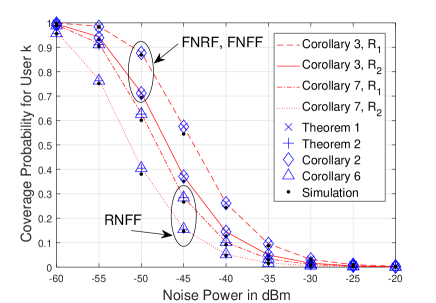
(a) Coverage probability for User $k$ versus noise, with the first range $R_{1}$: $a_{k}=0.4,a_{j}=0.6,\tau_{k}=1,\tau_{j}=1$, and the second range $R_{2}$: $a_{k}=0.1,a_{j}=0.9,\tau_{k}=1,\tau_{j}=0.2$.

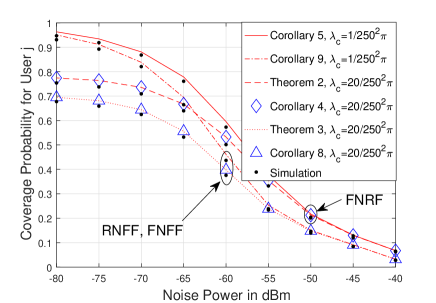
(b) Coverage probability for User $j$ versus noise, with the conditions: $a_{k}=0.1,a_{j}=0.9,\tau_{k}=1$, and $\tau_{j}=0.2$.

Figure 2: Monte Carlo simulations and verifications.

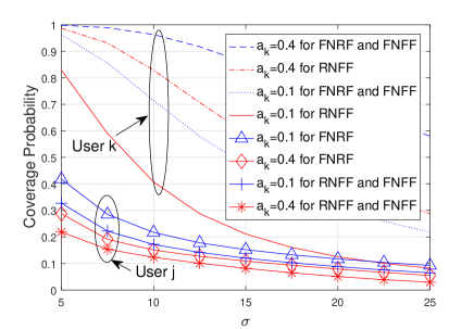
(a) Coverage probability for two paired users versus standard deviation $\sigma$, with $\tau_{k}=1$, $\tau_{j}=0.2$ and the noise power $-50$ dBm.

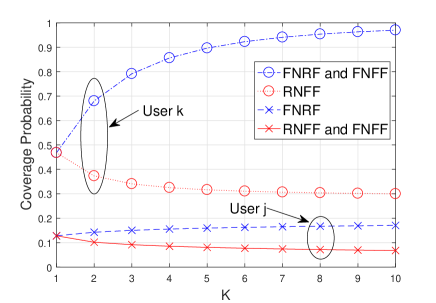
(b) Coverage probability for two paired users versus standard the number of pairs in one cluster $K$, with $a_{k}=0.2$, $a_{j}=0.8$, $\tau_{k}=1$, $\tau_{j}=0.2$, $\sigma=15$ and the noise power $-50$ dBm.

Figure 3: The impact of the system structure.

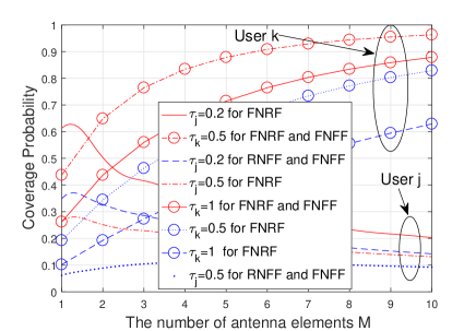
(a) Coverage probability for two paired users versus the number of antenna elements $M$, with the noise power $-50$ dBm, $a_{k}=0.2$ and $a_{j}=0.8$.

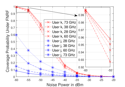
(b) Coverage probability under the FNRF scheme versus noise, with $a_{k}=0.1$, $a_{j}=0.9$, $\tau_{k}=1$ and $\tau_{j}=0.2$.

Figure 4: The effect of antenna scale and different carrier frequencies.

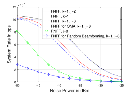
(a) System rate for OMA and NOMA versus noise, with $K=4$, $a_{k}=0.4$; $R_{k}=100$ Mbps and $R_{j}=30$ Mbps.

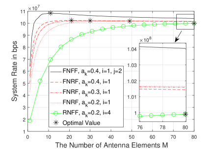
(b) System rate for three schemes versus the number of antenna elements $M$, with $R_{k}=100$ Mbps and $R_{j}=30$ Mbps.

Figure 5: The performance of system rate.

In addition to $\sigma$, the performance of coverage probabilities with different number of NOMA pairs $K$ is illustrated in Fig. 3(b). Two user selection strategies have totally inverse feedbacks. When $K=1$, three schemes are same as discussed in Remark 7 and Remark 9. With the rise of $K$, the coverage probabilities under the FNRF steadily increase, while that under the RNFF scheme is the opposite. Moreover, such probabilities for both strategies become flat when $K=9$, which implies even in a large cluster with massive pairs of NOMA users, the exact coverage performance can be tightly approximated by a more tractable scenario with smaller $K$.

V-C The Impact of Antenna Scale and Carrier Frequency

Regarding the antenna beamforming, two paired users have inverse performances as illustrated in Fig. 4(a). In general, the coverage probabilities of near users for three schemes are increasing functions with antenna scale $M$ as discussed in Remark 5 and Remark 8 , while those of far users are just the reverse. Due to the randomness of the channel vector $\bf{h_{j}}$, the coverage probability of User $j$ is fluctuant as mentioned in Remark 6 and Remark 9. The best choice for far user can be effortlessly figured out from Fig. 4(a) because of the convex property. Lastly, when the SINR threshold increases, the corresponding coverage probability decreases.

TABLE II: Path Loss Exponent for Different Carrier Frequencies

Carrier Frequencies	28G	38G	60G	73G
LOS $\alpha_{L}$	2	2	2.25	2
Strongest NLOS $\alpha_{N}$	3	3.71	3.76	3.4
Number of antenna elements $M$	10	20	40	80

Since mmWave has a large band of free available spectrum, we are interested in the performance of different carrier frequencies. The path loss exponents and estimated antenna scales [13] are shown in Table II. As the coverage performance for three schemes are same, we only demonstrate the FNRF scheme in Fig. 4(b). For User $k$, the best carrier frequency is 73 GHz due to the large antenna scale, while 60 GHz achieves the lowest in terms of coverage probability because of the highest $\alpha_{L}$. For User $j$, 28 GHz is the best choice and 73 GHz turns to be the worst one. Accordingly, the best choice of carrier frequency depends on the practical requirements for two paired users.

V-D Performance of System Throughput

We present the comparison of three schemes in terms of the system throughput in Fig. 5(a). It illustrates that the paired user with short communication distance has a high system rate. Therefore, the FNFF with $k=1$ and $j=2$ achieves the best performance. Then, compared with the OMA method under the FNFF scheme with $k=1$ and $j=8$, NOMA scenario performs better. Since the main beam is aligned towards User $k$, our schemes have an huge improvement when comparing with the random beamforming as mentioned in [34, 35]. However, our system needs the extra cost for acquiring SCI.

In terms of the number of antenna elements $M$ as shown in Fig. 5(b), there exists an optimal value that maximizes the system rate. The reason is that when $M$ is small, the beamwidth of the main beam is wide and hence User j has a high probability to be located in the coverage of the main beam. As a result, the system throughput rockets rapidly at first. Note that in general, the coverage probability of User $j$ decreases with the increase of $M$ as shown in Fig. 4(a). When $M$ is large, the impact of User $j$ is enhanced. Therefore, the system rate slightly decreases. Fig. 5(b) also illustrates that when $M$ is massive, the difference between three schemes becomes negligible regarding the system rate.

V-E Evaluation of Gauss-Chebyshev Quadrature

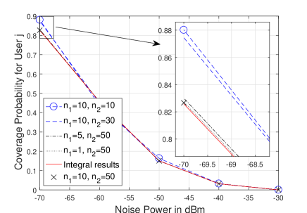
Figure 6: Coverage probability for User $j$ versus the noise power with the aid of Corollary 8, with $j=4$, $a_{k}=0.1,a_{j}=0.9,\tau_{k}=1$ and $\tau_{j}=0.2$.

We apply Gauss-Chebyshev quadrature to provide a tight approximation of the coverage probability. In this part, we evaluate both the accuracy and efficiency of such method. Note that the exact expression of antenna gains is an integral as shown in (Appendix A: Proof of Lemma 4) and (Appendix C: Proof of Theorem 2). For User $j$, since the antenna beam directions of its serving BS and all interfering transmitters are randomly distributed, the final coverage probability should consider the expectations of both the serving and interfering antenna gains. This consideration results in a complex and time-consuming double integral, which can be simplified by Gauss-Chebyshev quadrature. We discuss Corollary 8 in Fig. 6 as a case study. It illustrates that the parameter $n_{1}$ in Lemma 5 impacts the final result negligibly, even the case $n_{1}=1$ is able to provide acceptable accuracy. Regarding the parameter $n_{2}$ in Corollary 8, when $n_{2}$ increases to $50$, the approximation ideally overlaps the exact result. As a conclusion, the small parameter of Gauss-Chebyshev quadrature is enough to support high accuracy and high efficient numerical analyses.

VI Conclusion

In this paper, we have proposed three user selection schemes in clustered mmWave networks with NOMA techniques. With the aid of stochastic geometry, analytical expressions for coverage and system throughput have been presented. In addition, we have derived closed-form equations for a sparse network, which can be utilized in numerous practical noise-limited scenarios. As demonstrated in previous sections, the coverage probability and system throughput for the FNRF scheme with $k=1$ outperforms those for the RNFF scheme with $j=2K$. Large variance $\sigma^{2}$ impairs the received SINR. Moreover, 73 GHz is the best carrier frequency for near user and 28 GHz is the best one for far user. Lastly, our NOMA system beats the traditional OMA case in terms of the system rate. There is an optimal value of antenna scale for achieving maximum system throughput. Lastly, based on the proposed spatial framework, the joint optimization of distance-dependent pairing strategies and the antenna beamforming patterns for various objectives, e.g., maximizing the sum rate, minimizing the interference, maximizing the data rate of the primary user, and so forth, will inspire future work.

Appendix A: Proof of Lemma 4

The inter-cluster interferences can be divided into two groups: LOS interferences and NLOS interferences. Therefore, for User $k$, the Laplace transform of interferences is defined as follows

$${\mathcal{L}_{I}^{k}}\left(s\right)= \mathbb{E}\left[{\exp\left({-s{I_{{{inter},k}}}}\right)}\right]$$

$$= \mathbb{E}\big{[}{\exp\big{(}{-s\sum\nolimits_{y\in\Phi\backslash{y_{0}}}M{{{\left|{{g_{y\to k}}}\right|}^{2}}{G_{F}}\left({{\theta_{k}}-{\theta_{{\xi_{y}}}}}\right)}}}$$

$$\times{{{L_{p}}\left({\left\|{{x_{k}}-y}\right\|}\right)}\big{)}}\big{]}.$$ (A.1)

By substituting (3) into (Appendix A: Proof of Lemma 4) and calculating the expectation of Gamma random variable $\left|{{g_{y\to k}}}\right|^{2}$, we have

$$\mathcal{L}_{I}^{k}\left(s\right)={\mathbb{E}_{{G_{F}}}}\Bigg{[}$$

$$\prod\limits_{y\in\Phi\backslash{y_{0}}}{{\mathbb{E}_{y}}}\bigg{[}{\Big{(}{\frac{{{N_{L}}}}{{sM{G_{F}}\left({{\theta_{k}}-{\theta_{{\xi_{y}}}}}\right)C_{L}{{\left\|{{x_{k}}-y}\right\|}^{-{\alpha_{L}}}}+{N_{L}}}}}\Big{)}^{{N_{L}}}}$$

$$\times\mathbf{U}\left({{R_{L}}-\left\|{{x_{k}}-y}\right\|}\right)$$

$$\times{\left({\frac{{{N_{N}}}}{{sM{G_{F}}\left({{\theta_{k}}-{\theta_{{\xi_{y}}}}}\right)C_{N}{{\left\|{{x_{k}}-y}\right\|}^{-{\alpha_{N}}}}+{N_{N}}}}}\right)^{{N_{N}}}}$$

$$\times\mathbf{U}\left({\left\|{{x_{k}}-y}\right\|-{R_{L}}}\right)\bigg{]}\Bigg{]}.$$ (A.2)

As the interfering BSs are distributed following PPP with density $\lambda_{c}$, (Appendix A: Proof of Lemma 4) can be further deduced by the probability generating functional of PPP [44] as follows

$$\mathcal{L}_{I}^{k}\left(s\right)={\mathbb{E}_{{G_{F}}}}\Bigg{[}$$

$$e^{{-2\pi{\lambda_{c}}\int_{0}^{{R_{L}}}{\left({1-{{\left({\frac{{{N_{L}}}}{{sM{G_{F}}\left({{\theta_{k}}-{\theta_{{\xi_{y}}}}}\right){C_{L}}{v^{-{\alpha_{L}}}}+{N_{L}}}}}\right)}^{{N_{L}}}}}\right)vdv}}}$$

$$\times e^{{-2\pi{\lambda_{c}}\int_{{R_{L}}}^{\infty}{\left({1-{{\left({\frac{{{N_{N}}}}{{sM{G_{F}}\left({{\theta_{k}}-{\theta_{{\xi_{y}}}}}\right){C_{N}}{v^{-{\alpha_{N}}}}+{N_{N}}}}}\right)}^{{N_{N}}}}}\right)vdv}}}\Bigg{]}$$ (A.3)

Then we calculate the expectation of the antenna beamforming $G_{F}(.)$. As $({\theta_{k}}-{\theta_{{\xi_{y}}}})$ is uniformly distributed over $[-1,1]$, we use $g$ to replace $({\theta_{k}}-{\theta_{{\xi_{y}}}})$ for simplifying the notation. Under this assumption, we obtain

$$\mathcal{L}_{I}^{k}\left(s\right)=\exp\Bigg{(}-\pi{\lambda_{c}}$$

$$\times\int_{-1}^{1}\bigg{(}\int_{0}^{{R_{L}}}{\left({1-{{\left({1+\frac{{sM{G_{F}}\left(g\right){C_{L}}}}{{{N_{L}}{v^{{\alpha_{L}}}}}}}\right)}^{-{N_{L}}}}}\right)vdv}$$

$$+\int_{{R_{L}}}^{\infty}{\left({1-{{\left({1+\frac{{sM{G_{F}}\left(g\right){C_{N}}}}{{{N_{N}}{v^{{\alpha_{N}}}}}}}\right)}^{-{N_{N}}}}}\right)vdv}\bigg{)}dg\Bigg{)}.$$ (A.4)

Note that $\mathcal{G}_{F}^{I}\left(.\right)$ is an even function in terms of $g$. By substituting (3.194-2) [50] and the definition of Gauss hypergeometric function [51] into (Appendix A: Proof of Lemma 4), we obtain

$$\mathcal{L}_{I}^{k}\left(s\right)=\exp\left({-2\pi{\lambda_{c}}R_{L}^{2}\int_{0}^{1}{\mathcal{G}_{F}^{I}\left(s,g\right)}dg}\right).$$ (A.5)

Note that the Laplace transform of interferences for User $j$ has the similar deducing procedure, so two paired users share the same expressions. Therefore we are able to drop the index $k$ from (A.5). After that, applying Gaussian-Chebyshev quadrature equation into (A.5), the proof of Lemma 4 is complete.

Appendix B: Proof of Theorem 1

Under the FNRF scheme, the coverage probability for near user User $k$ at $x_{k}$ is given by

$$P_{k}^{\rm FR}\left({{\tau_{k}},{\tau_{j}}}\right)= \mathbb{P}\left[{{\gamma_{k}}>{\tau_{k}},{\gamma_{k\to j}}>{\tau_{j}}}\right]$$

$$= \mathbb{P}\bigg{[}{\frac{{{a_{k}}M{{\left|{{g_{k}}}\right|}^{2}}{L_{p}}\left({\left\|{{x_{k}}}\right\|}\right)}}{{{I_{{\rm{inter}},k}}+\sigma_{n}^{2}}}>{\tau_{k}}}$$

$${\&{\frac{{{a_{j}}M{{\left|{{g_{k}}}\right|}^{2}}{L_{p}}\left({\left\|{{x_{k}}}\right\|}\right)}}{{{a_{k}}M{{\left|{{g_{k}}}\right|}^{2}}{L_{p}}\left({\left\|{{x_{k}}}\right\|}\right)+{I_{{\rm{inter}},k}}+\sigma_{n}^{2}}}>{\tau_{j}}}}\bigg{]}$$

$$= \mathbb{P}\Bigg{[}{{{\left|{{g_{k}}}\right|}^{2}}>\underbrace{\frac{{{\tau_{k}}\left({{I_{{\rm{inter}},k}}+\sigma_{n}^{2}}\right)}}{{{a_{k}}M{L_{p}}\left({\left\|{{x_{k}}}\right\|}\right)}}}_{{\Xi_{2}}}}$$

$${\&{{{\left|{{g_{k}}}\right|}^{2}}>\underbrace{\frac{{{\tau_{j}}\left({{I_{{\rm{inter}},k}}+\sigma_{n}^{2}}\right)}}{{\left({{a_{j}}-{\tau_{j}}{a_{k}}}\right)M{L_{p}}\left({\left\|{{x_{k}}}\right\|}\right)}}}_{{\Xi_{1}}}}}\Bigg{]}.$$ (B.1)

On the one hand, when ${a_{k}}{\tau_{j}}<{a_{j}}\leq{a_{k}}{\tau_{j}}\left({1+\frac{1}{{{\tau_{k}}}}}\right)$, ${{\Xi_{1}}}\geq{{\Xi_{2}}}$. Therefore (Appendix B: Proof of Theorem 1) can be changed into

$$P_{k}^{\rm FR}\left({{\tau_{k}},{\tau_{j}}}\right)$$

$$=\mathbb{P}\left[{{{\left|{{g_{k}}}\right|}^{2}}>\frac{{{\tau_{j}}\left({{I_{{\rm{inter}},k}}+\sigma_{n}^{2}}\right)}}{{\left({{a_{j}}-{\tau_{j}}{a_{k}}}\right)M{L_{p}}\left({r_{k}}\right)}},{r_{k}}=\left\|{{x_{k}}}\right\|}\right]$$

$$=\underbrace{{\mathbb{P}}\left[{{{\left|{{g_{k}}}\right|}^{2}}>\frac{{{\tau_{j}}\left({{I_{{\rm{inter}},k}}+\sigma_{n}^{2}}\right)r_{k}^{{\alpha_{L}}}}}{{\left({{a_{j}}-{\tau_{j}}{a_{k}}}\right)M{C_{L}}}},{r_{k}}\leq{R_{L}}}\right]}_{{\Omega_{L}}\left({{\tau_{k}},{\tau_{j}}}\right)}$$

$$+\underbrace{{\mathbb{P}}\left[{{{\left|{{g_{k}}}\right|}^{2}}>\frac{{{\tau_{j}}\left({{I_{{\rm{inter}},k}}+\sigma_{n}^{2}}\right)r_{k}^{{\alpha_{N}}}}}{{\left({{a_{j}}-{\tau_{j}}{a_{k}}}\right)M{C_{N}}}},{r_{k}}>{R_{L}}}\right]}_{{\Omega_{N}}\left({{\tau_{k}},{\tau_{j}}}\right)},$$ (B.2)

where ${{\Omega_{L}}\left(.\right)}$ and ${{\Omega_{L}}\left(.\right)}$ are the coverage probability for LOS and NLOS links, respectively. By applying the tight upper bound mentioned in [10] for the normalized gamma random variable $\left|{{g_{k}}}\right|^{2}$ and Laplace transform of interferences, we first deduce ${{\Omega_{L}}\left(.\right)}$ as follows

$${\Omega_{L}}\left({{\tau_{k}},{\tau_{j}}}\right)\approx$$

$$1-\mathbb{E}\left[{\left(1-\exp{{\left({-\frac{{{\psi_{L}}{\tau_{j}}\left({{I_{{\rm{inter}},k}}+\sigma_{n}^{2}}\right)r_{k}^{{\alpha_{L}}}}}{{\left({{a_{j}}-{\tau_{j}}{a_{k}}}\right)M{C_{L}}}}}\right)}^{{N_{L}}}}\right)}\right]$$

$$\times\mathbf{U}\left({{R_{L}}-{r_{k}}}\right)$$

$$=\int_{0}^{{R_{L}}}{{\Theta_{L}}\left({{r_{k}},{\tau_{j}},{a_{j}}-{\tau_{j}}{a_{k}}}\right)f_{\rm FR}^{k}\left({{r_{k}}}\right)d{r_{k}}}.$$ (B.3)

Utilizing the same method, we obtain

$${\Omega_{N}}\left({{\tau_{k}},{\tau_{j}}}\right)\approx\int_{{R_{L}}}^{\infty}{{\Theta_{N}}\left({{r_{1}},{\tau_{j}},{a_{j}}-{\tau_{j}}{a_{k}}}\right)f_{\rm FR}^{k}\left({{r_{k}}}\right)d{r_{k}}}.$$ (B.4)

Then, substituting (Appendix B: Proof of Theorem 1) and (B.4) into (Appendix B: Proof of Theorem 1), we have (1).

On the other hand, when ${a_{j}}>{a_{k}}{\tau_{j}}\left({1+\frac{1}{{{\tau_{k}}}}}\right)$, ${{\Xi_{1}}}<{{\Xi_{2}}}$. With the aid of similar proof procedure of the aforementioned range, we are able to derive (1). Finally, the proof of Theorem 1 is complete.

Appendix C: Proof of Theorem 2

Under the FNRF scheme, far user at $x_{j}$ is randomly selected from the rest further NOMA users, so it can be expressed as follows

$$P_{j}^{\rm FR}\left({{\tau_{j}}}\right)=\mathbb{P}\left[{{\gamma_{j}}>{\tau_{j}}}\right]$$

$$=\mathbb{P}\bigg{[}{\frac{{{a_{j}}M{{\left|{{g_{j}}}\right|}^{2}}{G_{F}}\left({{\theta_{k}}-{\theta_{j}}}\right){L_{p}}\left({{r_{j}}}\right)}}{{{a_{k}}M{{\left|{{g_{j}}}\right|}^{2}}{G_{F}}\left({{\theta_{k}}-{\theta_{j}}}\right){L_{p}}\left({{r_{j}}}\right)+{I_{{\rm{inter}},j}}+\sigma_{n}^{2}}}>{\tau_{j}}},$$

$${{{r_{j}}\geq{r_{k}},{r_{k}}=\left\|{{x_{k}}}\right\|}}\bigg{]}$$

$$=\mathbb{P}\bigg{[}{{{\left|{{g_{j}}}\right|}^{2}}>\frac{{{\tau_{j}}\left({{I_{{\rm{inter}},j}}+\sigma_{n}^{2}}\right)}}{{M{G_{F}}\left({{\theta_{k}}-{\theta_{j}}}\right){L_{p}}\left({{r_{j}}}\right)\left({{a_{j}}-{\tau_{j}}{a_{k}}}\right)}}},$$

$${{{r_{j}}\geq{r_{k}},{r_{k}}=\left\|{{x_{k}}}\right\|}}\bigg{]}.$$ (C.1)

With the similar method as discussed in (Appendix B: Proof of Theorem 1) and (Appendix B: Proof of Theorem 1), we divide the probability into LOS links and NLOS links. Then the probability for LOS links is given by

$$\mathbb{P}\bigg{[}{{{\left|{{g_{j}}}\right|}^{2}}>\frac{{{\tau_{j}}\left({{I_{{\rm{inter}},j}}+\sigma_{n}^{2}}\right)}}{{M{G_{F}}\left({{\theta_{k}}-{\theta_{j}}}\right){L_{p}}\left({{r_{j}}}\right)\left({{a_{j}}-{\tau_{j}}{a_{k}}}\right)}}},$$

$${{{r_{j}}\geq{r_{k}},{r_{k}}\leq{R_{L}}}}\bigg{]}$$

$$\approx\int_{0}^{{R_{L}}}{\int_{{r_{k}}}^{{R_{L}}}{\Big{(}{1-\mathbb{E}\Big{[}{1-e^{{\left({-\frac{{{\psi_{L}}{\tau_{j}}\left({{I_{{\rm{inter}},j}}+\sigma_{n}^{2}}\right)r_{f}^{{\alpha_{L}}}}}{{M{G_{F}}\left({{\theta_{k}}-{\theta_{j}}}\right)\left({{a_{j}}-{\tau_{j}}{a_{k}}}\right){C_{L}}}}}\right)}^{{N_{L}}}}}\Big{]}}\Big{)}}}$$

$$\times{f_{\rm FR}^{j}\left({{r_{j}}}\right)d{r_{j}}}f_{\rm FR}^{k}\left({{r_{k}}}\right)dr_{k}$$

$$=\frac{1}{{2}}\int_{-1}^{1}{\int_{0}^{{R_{L}}}{\int_{{r_{k}}}^{{R_{L}}}{{\Theta_{L}}\left({{r_{f}},{\tau_{j}},\left({{a_{j}}-{\tau_{j}}{a_{k}}}\right){G_{F}}\left(g\right)}\right)}}}$$

$$\times{{f_{\rm FR}^{j}\left({{r_{j}}}\right)d{r_{j}}}f_{\rm FR}^{k}\left({{r_{k}}}\right)dr_{k}dg},$$ (C.2)

where $g$ represents $({{\theta_{k}}-{\theta_{j}}})$. On the other hand, the probability for NLOS links is expressed as follows

$$\mathbb{P}\bigg{[}{{{\left|{{g_{j}}}\right|}^{2}}>\frac{{{\tau_{j}}\left({{I_{{\rm{inter}},j}}+\sigma_{n}^{2}}\right)}}{{M{G_{F}}\left({{\theta_{k}}-{\theta_{j}}}\right){L_{p}}\left({{r_{j}}}\right)\left({{a_{j}}-{\tau_{j}}{a_{k}}}\right)}}},$$

$${{{r_{j}f}\geq{r_{k}},{r_{k}}>{R_{L}}}}\bigg{]}$$

$$\approx \int_{0}^{1}{\int_{{R_{L}}}^{\infty}{\int_{{r_{k}}}^{\infty}{{\Theta_{N}}\left({{r_{j}},{\tau_{j}},\left({{a_{j}}-{\tau_{j}}{a_{k}}}\right){G_{F}}\left(g\right)}\right)}}}$$

$$\times{{f_{\rm FR}^{j}\left({{r_{j}}}\right)d{r_{j}}}f_{\rm FR}^{k}\left({{r_{k}}}\right)dr_{k}dg}.$$ (C.3)

By substituting (Appendix C: Proof of Theorem 2) and (Appendix C: Proof of Theorem 2) into (Appendix C: Proof of Theorem 2) and then applying Gaussian-Chebyshev quadrature equation, we obtain Theorem 2. The proof is complete.

Appendix D: Proof of Corollary 7

With the similar proof in (Appendix C: Proof of Theorem 2), for range $R_{1}$, the coverage probability of User $k$ under special case 2 is given by

$$\hat{P}_{k}^{\rm RF}\left({{\tau_{k}},{\tau_{j}}}\right)\approx \int_{0}^{{R_{L}}}{\int_{0}^{{r_{j}}}{{{\hat{\Theta}}_{L}}\left({{r_{k}},{\tau_{j}},{a_{j}}-{\tau_{j}}{a_{k}}}\right)}}$$

$${\times f_{\rm RF}^{k}\left({{r_{k}}|{r_{j}}}\right)dr_{k}f_{\rm RF}^{j}\left({{r_{j}}}\right)d{r_{j}}},$$ (D.1)

where ${{\hat{\Theta}}_{L}}\left(.\right){\rm{=}}{\Theta_{L}}\left(.\right)\left|{{}_{\mathcal{L}_{I}\left(.\right)\to\tilde{\mathcal{L}}_{I}\left(.\right)}}\right.$. By substituting (22) and (25) into (Appendix D: Proof of Corollary 7), we obtain

$$\hat{P}_{k}^{\rm RF}\left({{\tau_{k}},{\tau_{j}}}\right)\approx\int_{0}^{{R_{L}}}{\sum\limits_{{n_{L}}=1}^{{N_{L}}}{\sum\limits_{w=0}^{k-1}{{{\left({-1}\right)}^{{n_{L}}+k-w}}{{k-1}\choose w}}{N_{L}\choose n_{L}}}}$$

$$\times{\frac{\Gamma_{k}}{{\sigma^{4}}{{A_{3}}\left({{\tau_{j}}}\right)}}\frac{{{r_{j}}\left({\exp\left({-Ar_{j}^{2}}\right)-\exp\left({-Br_{j}^{2}}\right)}\right)}}{{1-\exp\left({-Cr_{j}^{2}}\right)}}d{r_{j}}},$$ (D.2)

where $A=\frac{{\left({2K-w}\right)}}{{2{\sigma^{2}}}}$, $B=\frac{{\left({2K-w}\right)}}{{2{\sigma^{2}}}}+{A_{3}}\left({{\tau_{j}}}\right)$ and $C=\frac{1}{{2{\sigma^{2}}}}$. We first figure out a special integral in the following part.

$$\int_{0}^{{R_{L}}}{\frac{{r\left({\exp\left({-A{r^{2}}}\right)-\exp\left({-B{r^{2}}}\right)}\right)}}{{1-\exp\left({-C{r^{2}}}\right)}}dr}$$

$$= \frac{1}{{2C}}\Bigg{(}{\int_{0}^{1}{\frac{{{t^{\frac{A}{C}-1}}-{t^{\frac{B}{C}-1}}}}{{\left({1-t}\right)}}dt-\int_{0}^{\exp\left({-CR_{L}^{2}}\right)}{\frac{{{t^{\frac{A}{C}-1}}}}{{\left({1-t}\right)}}dt}}}$$

$${{+\int_{0}^{\exp\left({-CR_{L}^{2}}\right)}{\frac{{{t^{\frac{B}{C}-1}}}}{{\left({1-t}\right)}}dt}}}\Bigg{)}$$

$$\mathop{=}\limits^{(a)} \frac{1}{{2C}}\Big{(}\varphi\left({\frac{B}{C}}\right)-\varphi\left({\frac{A}{C}}\right)-\frac{{C\exp\left({-AR_{L}^{2}}\right)}}{A}$$

$$\times{}_{2}{F_{1}}\left({1,\frac{A}{C};1+\frac{A}{C};\exp\left({-CR_{L}^{2}}\right)}\right)$$

$$+\frac{{C\exp\left({-BR_{L}^{2}}\right)}}{B}{}_{2}{F_{1}}\left({1,\frac{B}{C};1+\frac{B}{C};\exp\left({-CR_{L}^{2}}\right)}\right)\Big{)}$$

$$\mathop{\approx}\limits^{(b)} \frac{1}{{2C}}\bigg{(}{\varphi\left({\frac{B}{C}}\right)-\varphi\left({\frac{A}{C}}\right)-\frac{{C\exp\left({-AR_{L}^{2}}\right)}}{A}}$$

$${+\frac{{C\exp\left({-BR_{L}^{2}}\right)}}{B}}\bigg{)}.$$ (D.3)

(a) follows (3.268-2) in [50] and the definition of Gauss hypergeometric function. (b) follows the fact $(\exp(-CR_{L}^{2})\approx 0)$ so that $({}_{2}{F_{1}}\left({.,.;.;\exp\left({-CR_{L}^{2}}\right)}\right)\approx 1)$. Then using (Appendix D: Proof of Corollary 7) into (Appendix D: Proof of Corollary 7), we obtain the expression for $R_{1}$ in Corollary 7. With the same method, we derive the equation for $R_{2}$ as well. The proof is complete.

References

• [1] W. Yi, Y. Liu, and A. Nallanathan, “Exploiting multiple access in clustered millimeter wave networks: NOMA or OMA?” in IEEE Proc. of International Commun. Conf. (ICC), May 2018.
• [2] Z. Qin, J. Fan, Y. Liu, Y. Gao, and G. Y. Li, “Sparse representation for wireless communications: A compressive sensing approach,” IEEE Signal Process. Mag., vol. 35, no. 3, pp. 40–58, May 2018.
• [3] Z. Qin, Y. Gao, M. D. Plumbley, and C. G. Parini, “Wideband spectrum sensing on real-time signals at sub-Nyquist sampling rates in single and cooperative multiple nodes,” IEEE Trans. Signal Process., vol. 64, no. 12, pp. 3106–3117, Jun. 2016.
• [4] J. G. Andrews, S. Buzzi, W. Choi, S. V. Hanly, A. Lozano, A. C. Soong, and J. C. Zhang, “What will 5G be?” IEEE J. Sel. Areas Commun., vol. 32, no. 6, pp. 1065–1082, Jun. 2014.
• [5] F. Boccardi, R. W. Heath, A. Lozano, T. L. Marzetta, and P. Popovski, “Five disruptive technology directions for 5G,” IEEE Commun. Mag., vol. 52, no. 2, pp. 74–80, Feb. 2014.
• [6] T. S. Rappaport, R. W. Heath Jr, R. C. Daniels, and J. N. Murdock, Millimeter Wave Wireless Communications.   Pearson Education, 2014.
• [7] “IEEE Standard for Information technology–Telecommunications and information exchange between systems–Local and metropolitan area networks–Specific requirements-Part 11: Wireless LAN Medium Access Control (MAC) and Physical Layer (PHY) Specifications Amendment 3: Enhancements for Very High Throughput in the 60 GHz Band,” IEEE Standard 802.11ad-2012, pp. 1–628, Dec. 2012.
• [8] T. Baykas, C. S. Sum, Z. Lan, J. Wang, M. A. Rahman, H. Harada, and S. Kato, “IEEE 802.15.3c: the first IEEE wireless standard for data rates over 1 Gb/s,” IEEE Commun. Mag., vol. 49, no. 7, pp. 114–121, Jul. 2011.
• [9] IEEE Standard for WirelessMAN-Advanced Air Interface of Broadband Wireless Access Systems, 2012.
• [10] T. Bai and R. W. Heath, “Coverage and rate analysis for millimeter-wave cellular networks,” IEEE Trans. Wireless Commun., vol. 14, no. 2, pp. 1100–1114, Feb. 2015.
• [11] T. S. Rappaport, F. Gutierrez, E. Ben-Dor, J. N. Murdock, Y. Qiao, and J. I. Tamir, “Broadband millimeter-wave propagation measurements and models using adaptive-beam antennas for outdoor urban cellular communications,” IEEE Trans. Antennas Propag., vol. 61, no. 4, pp. 1850–1859, Apr. 2013.
• [12] T. S. Rappaport, S. Sun, R. Mayzus, H. Zhao, Y. Azar, K. Wang, G. N. Wong, J. K. Schulz, M. Samimi, and F. Gutierrez, “Millimeter wave mobile communications for 5G cellular: It will work!” IEEE Access, vol. 1, pp. 335–349, May 2013.
• [13] W. Yi, Y. Liu, and A. Nallanathan, “Modeling and analysis of D2D millimeter-wave networks with Poisson cluster processes,” IEEE Trans. Commun., vol. 65, no. 12, pp. 5574–5588, Dec. 2017.
• [14] Z. Pi and F. Khan, “An introduction to millimeter-wave mobile broadband systems,” IEEE Commun. Mag., vol. 49, no. 6, Jun. 2011.
• [15] S. Akoum, O. E. Ayach, and R. W. Heath, “Coverage and capacity in mmWave cellular systems,” in Proc. 46th ASILOMAR, Nov. 2012, pp. 688–692.
• [16] G. Lee, Y. Sung, and J. Seo, “Randomly-directional beamforming in millimeter-wave multiuser MISO downlink,” IEEE Trans. Wireless Commun., vol. 15, no. 2, pp. 1086–1100, Feb. 2016.
• [17] D. Maamari, N. Devroye, and D. Tuninetti, “Coverage in mmWave cellular networks with base station co-operation,” IEEE Trans. Wireless Commun., vol. 15, no. 4, pp. 2981–2994, Apr. 2016.
• [18] J. G. Andrews, T. Bai, M. N. Kulkarni, A. Alkhateeb, A. K. Gupta, and R. W. Heath, “Modeling and analyzing millimeter wave cellular systems,” IEEE Trans. Commun., vol. 65, no. 1, pp. 403–430, Jan. 2017.
• [19] C. Park and T. S. Rappaport, “Short-range wireless communications for next-generation networks: UWB, 60 GHz millimeter-wave WPAN, and ZigBee,” IEEE Trans. Wireless Commun., vol. 14, no. 4, Aug. 2007.
• [20] R. Q. Hu and Y. Qian, “An energy efficient and spectrum efficient wireless heterogeneous network framework for 5G systems,” IEEE Commun. Mag., vol. 52, no. 5, pp. 94–101, May 2014.
• [21] Z. Ding, P. Fan, and H. V. Poor, “Impact of user pairing on 5G nonorthogonal multiple-access downlink transmissions,” IEEE Trans. Veh. Technol., vol. 65, no. 8, pp. 6010–6023, Aug. 2016.
• [22] Z. Ding, Y. Liu, J. Choi, Q. Sun, M. Elkashlan, C.-L. I, and H. V. Poor, “Application of non-orthogonal multiple access in LTE and 5G networks,” IEEE Commun. Mag., Feb. 2017.
• [23] Y. Liu, Z. Ding, M. Elkashlan, and J. Yuan, “Nonorthogonal multiple access in large-scale underlay cognitive radio networks,” IEEE Trans. Veh. Technol., vol. 65, no. 12, pp. 10 152–10 157, Dec 2016.
• [24] T. M. Cover and J. A. Thomas, Elements of Information Theory.   2nd ed. New York, NY, USA: Wiley, 2006.
• [25] Y. Liu, Z. Qin, M. Elkashlan, Z. Ding, A. Nallanathan, and L. Hanzo, “Nonorthogonal multiple access for 5G and beyond,” Proceedings of the IEEE, vol. 105, no. 12, pp. 2347–2381, Dec. 2017.
• [26] P. Xu, Y. Yuan, Z. Ding, X. Dai, and R. Schober, “On the outage performance of non-orthogonal multiple access with 1-bit feedback,” IEEE Trans. Wireless Commun., vol. 15, no. 10, pp. 6716–6730, Oct. 2016.
• [27] Z. Qin, X. Yue, Y. Liu, Z. Ding, and A. Nallanathan, “User association and resource allocation in unified NOMA enabled heterogeneous ultra dense networks,” IEEE Commun. Mag., vol. 56, no. 6, pp. 86–92, Jun. 2018.
• [28] Z. Ding, Z. Yang, P. Fan, and H. V. Poor, “On the performance of non-orthogonal multiple access in 5G systems with randomly deployed users,” IEEE Signal Process. Lett., vol. 21, no. 12, pp. 1501–1505, Dec. 2014.
• [29] Y. Liu, Z. Ding, M. Elkashlan, and H. V. Poor, “Cooperative non-orthogonal multiple access with simultaneous wireless information and power transfer,” IEEE J. Sel. Areas Commun., vol. 34, no. 4, pp. 938–953, Apr. 2016.
• [30] Y. Liu, Z. Qin, M. Elkashlan, Y. Gao, and L. Hanzo, “Enhancing the physical layer security of non-orthogonal multiple access in large-scale networks,” IEEE Trans. Wireless Commun., vol. 16, no. 3, pp. 1656–1672, Mar. 2017.
• [31] S. Timotheou and I. Krikidis, “Fairness for non-orthogonal multiple access in 5G systems,” IEEE Signal Process. Lett., vol. 22, no. 10, pp. 1647–1651, Oct. 2015.
• [32] N. Zhang, J. Wang, G. Kang, and Y. Liu, “Uplink nonorthogonal multiple access in 5G systems,” IEEE Commun. Lett., vol. 20, no. 3, pp. 458–461, Mar. 2016.
• [33] Y. Liu, Z. Qin, M. Elkashlan, A. Nallanathan, and J. A. McCann, “Non-orthogonal multiple access in large-scale heterogeneous networks,” IEEE J. Sel. Areas Commun., vol. 35, no. 12, pp. 2667–2680, Dec. 2017.
• [34] Z. Ding, P. Fan, and H. V. Poor, “Random beamforming in millimeter-wave NOMA networks,” IEEE Access, vol. 5, pp. 7667–7681, 2017.
• [35] J. Cui, Y. Liu, Z. Ding, P. Fan, and A. Nallanathan, “Optimal user scheduling and power allocation for millimeter wave NOMA systems,” IEEE Trans. Wireless Commun., vol. 17, no. 3, pp. 1502–1517, Mar. 2018.
• [36] Z. Xiao, L. Zhu, J. Choi, P. Xia, and X. Xia, “Joint power allocation and beamforming for non-orthogonal multiple access (NOMA) in 5G millimeter wave communications,” IEEE Trans. Wireless Commun., vol. 17, no. 5, pp. 2961–2974, May 2018.
• [37] L. Zhu, J. Zhang, Z. Xiao, X. Cao, D. O. Wu, and X. Xia, “Joint power control and beamforming for uplink non-orthogonal multiple access in 5G millimeter-wave communications,” IEEE Trans. Wireless Commun., vol. 17, no. 9, pp. 6177–6189, Sep. 2018.
• [38] K. Han and K. Huang, “Wirelessly powered backscatter communication networks: Modeling, coverage, and capacity,” IEEE Trans. Wireless Commun., vol. 16, no. 4, pp. 2548–2561, April 2017.
• [39] B. François and B. Bartłomiej, Stochastic geometry and wireless networks: Volume i theory.   NoW PublishersBreda, 2009.
• [40] R. K. Ganti and M. Haenggi, “Interference and outage in clustered wireless ad hoc networks,” IEEE Trans. Inf. Theory, vol. 55, no. 9, pp. 4067–4086, 2009.
• [41] S. Singh, M. N. Kulkarni, A. Ghosh, and J. G. Andrews, “Tractable model for rate in self-backhauled millimeter wave cellular networks,” IEEE J. Sel. Areas Commun., vol. 33, no. 10, pp. 2196–2211, Oct. 2015.
• [42] M. R. Akdeniz, Y. Liu, M. K. Samimi, S. Sun, S. Rangan, T. S. Rappaport, and E. Erkip, “Millimeter wave channel modeling and cellular capacity evaluation,” IEEE J. Sel. Areas Commun., vol. 32, no. 6, pp. 1164–1179, Jun. 2014.
• [43] H. A. David and H. N. Nagaraja, “Order statistics,” Encyclopedia of Statistical Sciences, vol. 9, 2004.
• [44] D. Stoyan, W. Kendall, and J. Mecke, “Stochastic geometry and its applications. 1995,” Akademie-Verlag, Berlin.
• [45] A. Ghosh, T. A. Thomas, M. C. Cudak, R. Ratasuk, P. Moorut, F. W. Vook, T. S. Rappaport, G. R. MacCartney, S. Sun, and S. Nie, “Millimeter-wave enhanced local area systems: A high-data-rate approach for future wireless networks,” IEEE J. Sel. Areas Commun., vol. 32, no. 6, pp. 1152–1163, Jun. 2014.
• [46] Y. Azar, G. N. Wong, K. Wang, R. Mayzus, J. K. Schulz, H. Zhao, F. Gutierrez, D. Hwang, and T. S. Rappaport, “28 GHz propagation measurements for outdoor cellular communications using steerable beam antennas in New York city,” in IEEE Proc. of International Commun. Conf. (ICC), Jun. 2013, pp. 5143–5147.
• [47] T. S. Rappaport, E. Ben-Dor, J. N. Murdock, and Y. Qiao, “38 GHz and 60 GHz angle-dependent propagation for cellular & peer-to-peer wireless communications,” in IEEE Proc. of International Commun. Conf. (ICC), Jun. 2012, pp. 4568–4573.
• [48] A. Thornburg, T. Bai, and R. W. Heath, “Performance analysis of outdoor mmWave ad hoc networks,” IEEE Trans. Signal Process., vol. 64, no. 15, pp. 4065–4079, Aug. 2016.
• [49] W. Yi, Y. Liu, and A. Nallanathan, “Cache-enabled HetNets with millimeter wave small cells,” IEEE Trans. Wireless Commun., vol. 66, no. 11, pp. 5497–5511, Nov. 2018.
• [50] A. Jeffrey and D. Zwillinger, Table of integrals, series, and products.   Academic press, 2007.
• [51] D. Liu and C. Yang, “Caching policy toward maximal success probability and area spectral efficiency of cache-enabled HetNets,” IEEE Trans. Commun., vol. 65, no. 6, pp. 2699–2714, Jun. 2017.
• [52] X. Yu, J. Zhang, M. Haenggi, and K. B. Letaief, “Coverage analysis for millimeter wave networks: The impact of directional antenna arrays,” IEEE J. Sel. Areas Commun., vol. 35, no. 7, pp. 1498–1512, Jul. 2017.