Overbooking Microservices in the Cloud

Abstract

We consider the problem of scheduling serverless-computing instances such as Amazon Lambda functions, or scheduling microservices within (privately held) virtual machines (VMs). Instead of a quota per tenant/customer, we assume demand for Lambda functions is modulated by token-bucket mechanisms per tenant. Such quotas are due to, e.g., limited resources (as in a fog/edge-cloud context) or to prevent excessive unauthorized invocation of numerous instances by malware. Based on an upper bound on the stationary number of active “Lambda servers” considering the execution-time distribution of Lambda functions, we describe an approach that the cloud could use to overbook Lambda functions for improved utilization of IT resources. An earlier bound for a single service tier is extended to multiple service tiers. For the context of scheduling microservices in a private setting, the framework could be used to determine the required VM resources for a token-bucket constrained workload stream. Finally, we note that the looser Markov inequality may be useful in settings where the job service times are dependent.

I Introduction

Public-cloud computing is conducted through Service-Level Agreements (SLAs), including pricing policies. Also, there is limited information-sharing regarding workloads between tenants and the operator/provider of a neutral public cloud [11]. Though public-cloud operators may seek to maximize their revenue and minimize their operating (including amortized capital) expenditures, they may be forced to treat tenants “fairly” according to future neutrality regulations. Moreover, it may not be permitted to profile individual tenants, though it may be permitted to profile, e.g., a particular service spanning all tenants that use it.

A variety of cloud-computing services have been broadly classified as Infrastructure-as-a-Service (IaaS) such as Virtual Machines (VMs), Platform-as-a-Service (PaaS) including Function-as-a-Service (FaaS) such as Amazon Lambda “serverless” computing, and Software-as-a-Service (SaaS) such as GCE’s TensorFlow. We focus herein on PaaS as offered by AWS (Lambda), GCE, Azure and IBM Cloud. In the following, we will call PaaS invocations Lambda functions or Lambda service instances.

Rather than renting reserved resources through a VM, under serverless computing multiple stateless Lambda functions are submitted by a tenant for execution in a provisioned container. AWS Lambda service tiers are based on 128MB units of memory, with 2 vCPU allocated per 3GB memory ($\frac{1}{12}$ vCPU per memory unit). Cost per tier is based on units of memory times the time that the Lambda invocation is active. State spanning plural Lambda invocations is externalized, e.g., managed by a “master” or “driver” VM or stored in AWS S3 or Single Queue Service (SQS); also see [9].

Lambda service instances typically require on the order of tens of milliseconds to a few minutes execution time [20, 18, 2]; in the lower range of execution times, cold-start spin-up overhead (including data acquisition) can be substantial. But to avoid such delays, a (cloud controlled) container may persist after a Lambda function finishes execution in anticipation of additional demand by the same tenant [20]. However, reserving the IT resources of dormant/paused containers for future invocations by the same tenant could be very resource inefficient.

In the following, we assume that an idle IT resource bundle for Lambda service, considered to be a “Lambda server”, can be used by any tenant at any time as permitted by their SLA. A disadvantage is that there may not be sufficient isolation among different cloud tenants under this assumption [13], e.g., presently, important data may be leaked from one tenant (whose Lambda function terminates) to another (whose Lambda function shortly thereafter commences in the same cloud-managed VM) through memory side-channels (i.e., the memory used by a Lambda function is not erased, or an equivalent operation performed, upon its termination).

Some providers limit the number of simultaneous cloud-function service-instances per tenant, e.g., AWS concurrency limits are described in [1]. There are security and cost risks to the tenant associated with autoscaling due to faults, the actions of intrusive malware, deliberate Denial-of-Service (DoS) attacks, or due to nominal but unexpected resource congestion (flash crowds) [12]. Concurrency limits may control such risks.

A tenant may explore performance/cost tradeoffs (including security) for serverless computing by implementing the same function differently, e.g., to reduce memory use. We also note that burstable/bursting and spot/preemptible VMs are less expensive to rent, the former having only intermittently available CPU (and network I/O) resources as governed by a token-bucket mechanism [19].

Also, the cloud provider generally wishes to operate their infrastructure efficiently. Efficient cloud operation, and associated potential cost savings for tenants, will be particularly important in edge/fog computing settings where: prices are generally much higher, concurrency limits per tenant are likely to be stricter, and servers mounting Lambda functions are likely to be shared among different tenants (rather than dedicated to individual tenants).

This paper focuses on the problem of cloud-side scheduling and consolidation of Lambda service instances, particularly principled approaches to overbook resources so as to improve utilization efficiency and thus maintain greatest possible service availability to tenant customers. So, from the tenant’s point of view, the edge-cloud Lambda service will be more dependable, particularly for autoscaling, notwithstanding congested (and costly) IT resources.

The following framework may also be useful in a more “private” setting-up of tenant-rented Virtual Machine (VM) resources housing containers executing a microservice-workload stream. Here, the aim could be to determine the number of VMs and their sizes so as to limit the amount of autoscaling while using these procured resources efficiently.

Finally, note that individual job service times may vary greatly, even in a microservice setting. So, limiting the job arrival stream by a token-bucket mechanism and just bounding the job execution times can lead to very inefficient use of resources. This motivates a simple statistical model for job service times. (Note that in packet switching, packet sizes are known a priori.)

This paper is organized as follows. Related work is discussed in Section II. The problem is set up in Section III and a no-blocking condition is given when a service quota is replaced by a token-bucket mechanism governing concurrency, i.e., governing how tenants may request homogeneous Lambda service instances. In Section IV, we show how admission control can be relaxed considering empirical Lambda-function execution times resulting in more efficient use of resources. An extension to multiple service tiers based in part on allocated resources per Lambda service instance is discussed in Section V. The paper concludes with a discussion of future work in Section VI.

II Related Work

For decades, token-bucket mechanisms have been used to control the resource utilization of a workload stream. In a packet-switching context, e.g., [4, 8, 7], the tasks (packet-header processing and packet transmission) have very predictable sizes compared to workloads of a general-purpose CPU, call center, etc. For scheduling purposes in the latter cases, token-bucket controls at the task level may be augmented by statistical models profiling task execution times, e.g., [10, 17, 6, 5]. In some cases, predictable workloads can be overbooked to improve resource-utilization efficiency. Some prior work on resource overbooking has been based on chance constraints, e.g., involving second-order statistics [11, 3].

Though we assume herein that Lambda-function invocations are limited by a deterministic token-buck mechanism, resource allocation to Lambda functions will also depend on the distribution of their execution times, as estimated by the cloud. Such estimates could be continually updated over time, as new Lambda-function execution-time statistics are collected. For example, a classical maximum-likelihood approach can be used to fit a sliding time-window of the most recent cloud-function execution times to a parameterized distribution model, e.g., of the Gamma [16] or Weibull type. In an online setting, if updates are based on observation batches, the old approximate service-time distribution, $\hat{p}$, and the one based on the most recent batch of observed Lambda execution/service times, $\hat{q}$, could be combined in a simple first-order autoregressive manner, $\alpha\hat{p}+(1-\alpha)\hat{q}$, where forgetting factor $\alpha$ is such that $0<\alpha<1$.

III Problem set-up and a no-blocking condition

Consider available resources of a set $\mathcal{I}$ of heterogeneous physical servers, including resources unused by existing IaaS instances (VMs). Let $c_{i,r}$ be the amount of IT resource of type $r\in\mathcal{R}$ (e.g., $\mathcal{R}=\{$vCPUs, memory, network I/O$\}$) available for Lambda service on server $i\in\mathcal{I}$. In the following, $\min_{r}$ will be short for $\min_{r\in\mathcal{R}}$, $\sum_{i}$ will be short for $\sum_{i\in\mathcal{I}}$, etc.

Consider a set $\mathcal{N}$ of tenant-customers of a common type of Lambda service, with $d_{r}$ being the amount of type $r\in\mathcal{R}$ resource allocated per invocation as prescribed by the SLA. In the following, we assume tenant SLAs stipulate

• IT resources allocated per invocation of the common type of Lambda service, $\{d_{r}\}_{r\in\mathcal{R}}$,

• a maximum execution/activity time $S_{\max}$ per invocation,

• and some limit to the rate at which tenants can request different Lambda service instances.

For the case of tenant demand for a single type of Lambda service, we can consider each available $|\mathcal{R}|$-vector of resources $\underline{d}$ from the physical server pool $\mathcal{I}$ as a “Lambda server” that pulls in work when idle, e.g., [15].

Suppose that there are $K$ such servers available:

$$K = \sum_{i\in\mathcal{I}}\min_{r\in\mathcal{R}}\left\lfloor\frac{c_{i,r}}{d_{r}}\right\rfloor.$$ (1)

Generally, $K$ is time-varying but at a longer time-scale than that of individual Lambda-service lifetimes or of the time between successive Lambda-service invocations.

III-A A quota system

First note that if there is a simple quota, $K_{n}<K$, on the number of active Lambda invocations for tenant $n$, then by Little’s formula, $K_{n}/{\sf E}S_{n}$ is an upper bound on the mean rate at which that tenant can request service, where the random variable $S_{n}$ is distributed as the execution time of tenant $n$’s Lambda functions. Furthermore, if tenant $n$’s service-request process is modeled as Poisson, then the Erlang blocking formula applies [21].

In the following, we do not assume a Poisson model for service request processes.

The cloud may overbook resources by, e.g., online estimating the mean and variance of the total number of active Lambda servers $Q\leq K$, respectively $\widehat{{\sf E}Q}$ and $\widehat{\mbox{var}(Q)}$, using, e.g., a simple autoregressive mechanism. Admission control could be based on the current 99%-confident estimate $K-\widehat{{\sf E}Q}-3\sqrt{\widehat{\mbox{var}(Q)}}$ of available Lambda servers. SLAs should capture how such overbooking approaches may sometimes result in blocking of within-quota requests for Lambda service.

III-B Demand constrained by token bucket regulators

Instead of a simple quota on the number of active invocations per tenant, the cloud can accommodate batch Lambda-service requests while effecting control on such a system by applying token-bucket allocators. For example, a dual token-bucket allocator permits only

$$g(t) = \min\{b+\pi t,~{}\sigma+\rho t\}$$ (2)

requests for Lambda service over any time-interval of length $t$, with peak rate larger than sustainable rate, $\pi>\rho>0$, and the maximum burst size at the sustainable rate greater than the number of simultaneous new Lambda-service requests that can be submitted, $\sigma>b$.

Note that, just as in a fixed quota system, every tenant is immediately aware of how many new Lambda service instances they can invoke at any given time based on their current token-bucket state.

Different tenants may engage in different service tiers $\mathcal{J}$ corresponding to different dual-token bucket mechanisms governing their rate of Lambda-service requests. Let $j(n)\in\mathcal{J}$ be the service tier of active tenant $n$ corresponding to burstiness curve $g_{j(n)}$. The maximum service time per Lambda-service invocation, $S_{j(n),\max}$, is also assumed to be stipulated in SLAs.

The following constraint

$$\sum_{n}g_{j(n)}(S_{j(n),\max}) \leq K$$ (3)

will imply that all Lambda-service requests satisfying (2) will be invoked upon request [4]. So, if the number of available servers is $K$, and $\mathcal{N}$ is the current set of active tenants, then a new tenant at service tier $j\in\mathcal{J}$ is admitted only if

$$g_{j}(S_{j,\max}) \leq K-\sum_{n\in\mathcal{N}}g_{j(n)}(S_{j(n),\max}).$$

If the tiers are designed so that there is an “atomic” tier $1\in\mathcal{J}$ based on its burstiness curve $g_{1}$ (i.e., for every tier $j\in\mathcal{J}$, $j$ is an integer such that $g_{j}=jg_{1}$), then a price $p_{j}$ for tier-$j$ invocations satisfying $p_{j}<jp_{1}$ would correspond to a volume discount.

IV Overbooking based on service-time distribution for a single service tier

Consider a single service tier. As (3) may be very conservative, the cloud may instead profile the service-time distribution $S$ across all tenants and service tiers and employ our Theorem 2 of [10] (reinterpreted in Appendix A). For an infinite server system, this result uses the Chernoff bound to show that the probability that the number of busy servers $Q$ exceeds $K$,

$${\sf P}(Q>K)~{}\leq~{}\Omega(\mathcal{N})~{}:=~{}\exp\Bigg{(}-\sup_{\theta>0}\Bigg{\{}\theta(K-g(0))$$ (4)

$$~{}~{}~{}-\int_{g(0)}^{g(S_{\max})}\log(\Phi(x)\mbox{e}^{\theta}+1-\Phi(x))\mbox{d}x\Bigg{\}}\Bigg{)},$$

where $\Phi(x):={\sf P}(g(S)>x)$ and $P(S=0)=0$ is assumed.

Note that the looser Markov inequality of Corollary VII.2 in Appendix A (relying only on common mean service times) does not require independent service times.

In the following, this theorem is extended to multiple service tiers.

If the distribution of $S$ based on recent Lambda-service invocations is continually estimated, then $\Phi$ and, in turn, the bound $\Omega(\mathcal{N})$ can be numerically computed for the given set of active tenants $\mathcal{N}$. If there is a small tolerable aggregate blocking probability of $\varepsilon>0$ (a quantity that could be stipulated in SLAs), a new tenant $n^{\prime}$ is admitted if

$$\Omega(\mathcal{N}\cup\{n^{\prime}\}) \leq \varepsilon,$$

here assuming that the new tenant $n^{\prime}$ will have negligible impact on the (collective) execution-time distribution.

Again, Lambda service instances typically require on the order of tens of milliseconds to a few minutes execution time [20, 18, 2]. For a numerical example, suppose the cloud models Lambda-service instances as having independent execution-times (lifetimes) $S$ that are (bell-shaped and non-negative) Weibull distributed with scale parameter 1 and shape parameter 5 so that the mean is 0.915 (minutes), and truncated so that $S_{\max}=1.4$ (at which point this Weibull density is approximately zero). Also suppose the collective burstiness curve is $g(t)=5+100t$, i.e., just a single token-bucket mechanism. Thus, the mean rate of invoked requests is less than 100 per second.

In one numerical example, we took two cases for demand. The first was a maximal $g$-permitted deterministic demand process wherein a batch of $5$ instance requests were made every $\frac{1}{20}$ second. In the second case, we simulated a Poisson process with mean rate 20 and batches of 5 instances were requested for each Poisson arrival. In the Poisson case, some requests did not satisfy the burstiness curve $g$ and were dropped so that the average admitted batch size was only $3.9$ (so, a mean rate of $20\times 3.9=78$ invoked requests per second). The mean number of occupied servers by simulation (or Little’s formula), ${\sf E}Q=92$ for deterministic batch requests and ${\sf E}Q=71$ for Poisson batch requests. Numerical results are given in Table I and Figures 1 and 2. We see that the Chernoff bound (4) does reasonably well indicating the number of required servers when the burstiness curves well reflect demand and blocking tolerance $\varepsilon$ is small, while (3) is very conservative even in this case.

We numerically found that the Markov inequality given in [10] (also see Appendix A), though much easier to compute than (4), is much more conservative even than (3). This said, it is relevant to cases where the service times $S_{i}$ are dependent (and ${\sf E}g(S)<K$, of course).

min $K$ s.t.
${\sf P}(Q>K)<.01=\varepsilon$	simulated	(4)	(3)
deterministic	100	108	145
Poisson	92	108	145

TABLE I: The minimum number of servers $K$ required so that ${\sf P}(Q>K)<0.01=\varepsilon$, i.e., the stationary probability that the number of occupied servers $Q>K$ is less than one percent, for simulated system and according to the Chernoff bound (4) and the no-blocking bound (3).

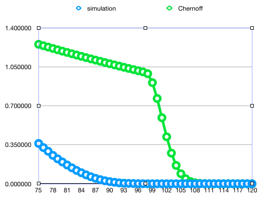
Figure 1: ${\sf P}(Q>K)$ evaluated by simulation and its Chernoff bound (4) versus $K$ for Poisson batch requests. Here ${\sf E}Q=71$.

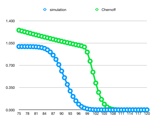
Figure 2: ${\sf P}(Q>K)$ evaluated by simulation and its Chernoff bound (4) versus $K$ for deterministic batch requests. Here ${\sf E}Q=92$.

IV-A Overbooking based on empirical weak burstiness curves on service-request process

The bound on blocking probability $\Omega(\mathcal{N})$ may still be conservative considering that many tenants may not request at close to the maximum rates given by (2) of their service tiers. To this end, an empirical service-request envelope $\hat{g}$ can be estimated for all currently active tenants, and $g$ can be replaced by $\hat{g}$ in the definition of $\Phi$. (That is, $\hat{g}$ can inform the burstiness curve requested by the tenant of the cloud.) Here, $\hat{g}$ can be any increasing, concave and nonnegative function.

To this end, consider the notion of a “weak” burstiness curve constraint involving a small positive confidence parameter $\delta<1$ [14]. Given the aggregate number of service requests over time interval $(s,t]$, $A(s,t]$, one can track virtual queues (e.g., [7, 8]) $V_{r}(t)=\max_{s\leq t}A(s,t]-r(t-s)$ for different service rates $r\leq\pi$. For each virtual queue, we can estimate minimal $\hat{\sigma}_{r}$ such that

$${\sf P}(V_{r}>\hat{\sigma}_{r}) < \delta.$$

In particular, the maximum simultaneous aggregate request observed $\hat{b}=\hat{\sigma}_{r}$ for $r=\pi$. Note that $\hat{\sigma}_{r}\leq\hat{\sigma}_{r^{\prime}}$ if $r>r^{\prime}$. Thus, we can approximate (concave)

$$\hat{g}(t) = \min_{r}\hat{\sigma}_{r}+tr.$$

V Discussion: Multiple service tiers for one resource pool

Consider the case where the aggregate demand of tier $j\in\mathcal{J}$ has service-request burstiness curve $g_{j}$ and i.i.d. execution-times $\sim S^{(j)}\leq S^{(j)}_{\max}$ such that ${\sf P}(S^{(j)}=0)=0$ $\forall j\in\mathcal{J}$. Assume arrival and service processes of each tier are mutually independent. Furthermore, suppose each Lambda service instance of type $j\in\mathcal{J}$ requires an amount $d_{j,r}$ of resource of type $r\in\mathcal{R}$. For all $j\in\mathcal{J}$ and $r\in\mathcal{R}$, let

$$q_{j,r} = Q_{j}d_{j,r}$$

be the total stationary amount of resource of type $r$ allocated to active Lambda service instances of type $j$ for an infinite resource system.

Assume that resources for Lambda service are from a single pool (physical server), $i$. Recall that the amount of type-$r$ resource available is $c_{i,r}$.

Corollary V.1

For physical server $i$,

$${\sf P}\left(\max_{r\in\mathcal{R}}\frac{\sum_{j}q_{j,r}}{c_{i,r}}>1\right)$$

$$\leq \exp\left(-\sup_{\theta>0}\left\{\theta-\sum_{j\in\mathcal{J}}\mathcal{M}_{j}\left(\theta\max_{r\in\mathcal{R}}\frac{d_{j,r}}{c_{i,r}}\right)\right\}\right)$$

where

$$\mathcal{M}_{j}(\theta)=\int_{g_{j}(0)}^{g_{j}(S^{(j)}_{\max})}\log(\Phi_{j}(x)\mbox{e}^{\theta}+1-\Phi_{j}(x))\mbox{d}x+\theta g_{j}(0)$$

and $\Phi_{j}(x)={\sf P}(g_{j}(S^{(j)})>x).$

Proof: For $\theta>0$,

$$\log{\sf E}\exp\left(\theta\max_{r}\frac{\sum_{j}q_{j,r}}{c_{i,r}}\right)$$

$$= \log{\sf E}\exp\left(\theta\max_{r}\sum_{j}\frac{Q_{j}d_{j,r}}{c_{i,r}}\right)$$

$$\leq \log{\sf E}\exp\left(\theta\sum_{j}Q_{j}\max_{r}\frac{d_{j,r}}{c_{i,r}}\right)$$

$$= \sum_{j}\log{\sf E}\exp\left(\theta Q_{j}\max_{r}\frac{d_{j,r}}{c_{i,r}}\right),$$

where the last equality is by assumed mutual independence of the $Q_{j}$, $j\in\mathcal{J}$. The proof then follows by the argument for the single-tier theorem (4) [10] (also see Appendix A) and the Chernoff bound. ∎

V-A An atomic service in terms of IT resources allocated

Consider the special case of an atomic service tier in terms of allocated resources (as in AWS Lambda). That is, suppose there are constants $\kappa_{j}$ such that

$$\forall j\in\mathcal{J},r\in\mathcal{R},~{}~{}d_{j,r} = \kappa_{j}d_{1,r}.$$ (5)

Regarding Corollary V.1 for this case, obviously

$$\forall j,~{}\max_{r}\frac{d_{j,r}}{c_{i,r}} = \kappa_{j}\max_{r}\frac{d_{1,r}}{c_{i,r}}.$$

Here, a tier-$j$ service instance would consume $\kappa_{j}$ tokens upon invocation.

V-B Extensions to multiple physical servers

To extend the case of multiple service tiers to multiple physical servers $i$, one can divide each tenant $n$’s demand envelope among them. For example, for nonnegative scalars $\alpha_{j(n),i}$ such that $\sum_{i}\alpha_{j(n),i}=1$, take $g_{j(n),i}=\alpha_{j(n),i}g_{j(n)}$ so that

$$g_{j(n)}=\sum_{i}g_{j(n),i}.$$

The weights $\alpha$ for each tenant can then be chosen to balance load among servers $i$. Given that, Corollary V.1 can be used for each server $i$.

Obviously, the above approach to admission control could be separately applied to each tier in $\mathcal{J}$ if resources for different service tiers are statically partitioned based on demand assessments.

Note that under (5), the price of type-$j$ Lambda service instances should be more than $\kappa_{j}$ type-1 (atomic) Lambda service instances because the former needs to be allocated on a single physical server.

VI Future Work

For longer running Lambda functions, if Lambda servers are available, it may be more resource efficient to invoke requests that violate their token-bucket profiles but flag them [8, 7] as preemptible or pausable. Also, blocked in-profile and out-of-profile requests may be temporarily queued. In future work, we will study the overhead of preemption and the performance of policies to price and preempt out-of-profile invocations.

Nonlinear chance constraints can replace linear “spatial” resource constraints such as (1). In future work, we will also consider how the above temporal approach to overbooking can be combined with instance-placement approaches based on chance constraints.

VII Appendix A: Loss system with arrivals satisfying burstiness curves

In this Appendix, we reinterpret the statement of Theorem 2 of [10] and provide a modified proof. Consider a bufferless system with $K\geq 1$ identical servers. Let $T_{i}$ be the arrival time of job (service request) $i$ and here let $S_{i}$ be its service time. Consider a (increasing, concave and nonnegative) burstiness curve $g$ for arrivals, i.e.,

$$\forall s\leq t,~{}~{}\sum_{i}{\bf 1}\{s<T_{i}\leq t\}\leq g(t-s).$$

Assume a maximum service time $S_{\max}$.

The number of busy servers (jobs in the system) at time $t$,

$$Q(t) = \sum_{i=-\infty}^{\infty}{\bf 1}\{T_{i}\leq t<T_{i}+S_{i}\}$$

$$= \sum_{i=-\infty}^{\infty}{\bf 1}\{t-S_{i}<T_{i}\leq t\}$$

$$\leq \sum_{i=-\infty}^{\infty}{\bf 1}\{t-S_{\max}<T_{i}\leq t\}$$

$$\leq g(S_{\max}).$$

So, if $g(S_{\max})\leq K$, then the $K$-server system will never block jobs [4].

Theorem VII.1

[10] If

$${\sf P}(S=0) = 0$$ (6)

and the service times $S_{i}$ are independent and identically distributed, then in steady-state,

$$\log{\sf E}\mbox{e}^{\theta Q} \leq \theta g(0)+$$

$$\int_{g(0)}^{g(S_{\max})}\log(\Phi(x)\mbox{e}^{\theta}+1-\Phi(x))\mbox{d}x$$

$$=: \mathcal{M}(\theta)$$

where $\Phi(x)={\sf P}(g(S)>x)$.

Corollary VII.1

If (6) and the $S_{i}$ are independent and identically distributed, then in steady-state the Chernoff bound is

$${\sf P}(Q>K) \leq \exp(-\sup_{\theta>0}\{\theta K-\mathcal{M}(\theta)\}).$$

Corollary VII.2

If (6) and the $S_{i}$ are identically distributed, then in steady-state the Markov inequality is,

$${\sf P}(Q>K) \leq \frac{{\sf E}g(S)}{K}.$$

Remark: For Corollary VII.2, the $S_{i}$ are not necessarily mutually independent.

Proof of the Theorem: Define a partition $\{m_{\ell}\}_{\ell=0}^{L+1}$ of the range of $g$:

$$m_{0}=g(0),~{}m_{\ell}<m_{\ell+1}~{}\forall\ell,~{}m_{L+1}=g(S_{\max}).$$

Define the job indexes so that $T_{-1}\leq t<T_{0}$ and

$$Q(t) = \sum_{i=-\infty}^{-1}{\bf 1}\{t-S_{i}<T_{i}\leq t\}.$$

Thus,

$$Q(t) = \sum_{i=-\infty}^{-1}\sum_{\ell=0}^{L}{\bf 1}\{t-S_{i}<T_{i}\leq t\}$$

$$~{}~{}\cdot{\bf 1}\{g^{-1}(m_{\ell})<S_{i}\leq g^{-1}(m_{\ell+1})\}$$

$$\leq \sum_{\ell=0}^{L}\sum_{i=-\infty}^{-1}{\bf 1}\{t-g^{-1}(m_{\ell+1})<T_{i}\leq t\}$$

$$~{}~{}\cdot{\bf 1}\{g^{-1}(m_{\ell})<S_{i}\leq g^{-1}(m_{\ell+1})\}$$

$$\leq \sum_{\ell=0}^{L}\sum_{i=-m_{\ell+1}}^{-1}{\bf 1}\{g^{-1}(m_{\ell})<S_{i}\leq g^{-1}(m_{\ell+1})\}$$

where the inequalities are by the burstiness constraint $g$ on $\{T_{i}\}$.

Switching the order of summation again gives,

$$Q(t) \leq \sum_{i=-m_{1}}^{-1}\sum_{\ell=0}^{L}{\bf 1}\{g^{-1}(m_{\ell})<S_{i}\leq g^{-1}(m_{\ell+1})\}$$

$$~{}~{}+\sum_{i=-m_{2}}^{-m_{1}-1}\sum_{\ell=1}^{L}{\bf 1}\{g^{-1}(m_{\ell})<S_{i}\leq g^{-1}(m_{\ell+1})\}$$

$$~{}~{}+...+\sum_{i=-m_{L+1}}^{-m_{L}-1}{\bf 1}\{g^{-1}(m_{L})<S_{i}\leq g^{-1}(m_{L+1})\}$$

$$= \sum_{i=-m_{1}}^{-1}{\bf 1}\{g^{-1}(m_{0})<S_{i}\}$$

$$~{}~{}+\sum_{i=-m_{2}}^{-m_{1}-1}{\bf 1}\{g^{-1}(m_{1})<S_{i}\}$$

$$~{}~{}+...+\sum_{i=-m_{L+1}}^{-m_{L}-1}{\bf 1}\{g^{-1}(m_{L})<S_{i}\}.$$

Taking expectation now and letting the partition $\{m_{\ell}\}_{\ell=0}^{L+1}$ become infinitely fine as $L\rightarrow\infty$ leads to ${\sf E}Q\leq{\sf E}\int_{g(0)}^{g(S_{\max})}{\sf P}(g(S)>x)\mbox{d}x={\sf E}g(S)$ and Corollary VII.2.

Continuing from the previous display: Since the $S_{i}$ are identically distributed $\sim S$,

$$\forall i,~{}~{}{\sf E}\exp(\theta{\bf 1}\{g^{-1}(m_{\ell})<S_{i}\}) = \Phi(m_{\ell})\mbox{e}^{\theta}+1-\Phi(m_{\ell}).$$

Since $S_{i}$ are independent and $\Phi(m_{0})=1$ (the latter because ${\sf P}(S=0)=0$),

$${\sf E}\mbox{e}^{Q(t)} \leq \mbox{e}^{\theta m_{0}}\prod_{\ell=0}^{L}(\Phi(m_{\ell})\mbox{e}^{\theta}+1-\Phi(m_{\ell}))^{m_{\ell+1}-m_{\ell}}$$

Thus,

$$\log{\sf E}\mbox{e}^{Q(t)}~{}\leq~{}\theta g(0)$$

$$+ \sum_{\ell=0}^{L}(m_{\ell+1}-m_{\ell})\log(\Phi(m_{\ell})\mbox{e}^{\theta}+1-\Phi(m_{\ell}))$$

So, as $L\rightarrow\infty$ and the partition $\{m_{\ell}\}$ of the range of $g$ becomes infinitely fine, this bound converges to the integral,

$$\theta g(0)+\int_{g(0)}^{g(S_{\max})}\log(\Phi(x)\mbox{e}^{\theta}+1-\Phi(x))\mbox{d}x~{}~{}~{}~{}\qed$$

References

- [1] AWS. AWS Lambda Function Scaling. https://docs.aws.amazon.com/lambda/latest/dg/concurrent-executions.html, 2019.
- [2] R.S. Barga. Serverless Computing - Redefining the Cloud. In Proc. WoSC, https://www.serverlesscomputing.org/wosc17/presentations/barga-keynote-serverless.pdf, 2017.
- [3] M.C. Cohen, V. Mirrokni, P. Keller, and M. Zadimoghaddam. Overcommitment in Cloud Services Bin packing with Chance Constraints. In Proc. ACM SIGMETRICS, Urbana-Campaign, IL, June 2017.
- [4] R.L. Cruz. Quality of service guarantees in virtual circuit switched networks. IEEE JSAC, Vol. 13, No. 6:pages 1048–1056, Aug. 1995.
- [5] C. Delimitrou and C. Kozyrakis. HCloud: Resource-Efficient Provisioning in Shared Cloud Systems. In Proc. ASPLOS, Atlanta, 2016.
- [6] C. Delimitrou and C. Kozyrakis. QoS-Aware Scheduling in Heterogeneous Datacenters with Paragon. ACM Trans. on Computer Systems, 31(4), Dec. 2013.
- [7] J. Heinanen, T. Finland, and R. Guerin. A single rate three color marker. RFC 2697 available at www.ietf.org, 1999.
- [8] J. Heinanen, T. Finland, and R. Guerin. A two rate three color marker. RFC 2698 available at www.ietf.org, 1999.
- [9] A. Jain, A.F. Baarzi, N. Alfares, G. Kesidis, B. Urgaonkar, and M. Kandemir. SplitServe: Efficient Splitting Complex Workloads across FaaS and IaaS, Nov. 2019; https://github.com/PSU-Cloud/splitserve-spark/blob/master/Paper/SplitServe.pdf.
- [10] G. Kesidis, K. Chakraborty, and L. Tassiulas. Traffic shaping for a loss system. IEEE Communication Letters, 4, No. 12:pp. 417–419, Dec. 2000.
- [11] G. Kesidis, N. Nasiriani, B. Urgaonkar, and C. Wang. Neutrality in Future Public Clouds: Implications and Challenges. In Proc. USENIX HotCloud, 2016.
- [12] E. Kim. Internal documents show how Amazon scrambled to fix Prime Day glitches. https://www.cnbc.com/2018/07/19/amazon-internal-documents-what-caused-prime-day-crash-company-scramble.html, July 19, 2018.
- [13] AWS Lambda. Security Overview of AWS Lambda. https://d1.awsstatic.com/whitepapers/Overview-AWS-Lambda-Security.pdf, March 2019.
- [14] S. Low and P. Varaiya. A simple theory of traffic resource allocation in ATM. In Proc. IEEE GLOBECOM, 1991.
- [15] G. McGrath and P.R. Brenner. Serverless computing: Design, implementation, and performance. In IEEE Int’l Conf. on Distributed Computing Systems Workshops, 2017.
- [16] T.P. Minka. Estimating a Gamma distribution. https://tminka.github.io/papers/minka-gamma.pdf, 2002.
- [17] Sergio Pacheco-Sanchez, Giuliano Casale, Bryan W. Scotney, Sally I. McClean, Gerard P. Parr, and Stephen Dawson. Markovian workload characterization for QoS prediction in the cloud. In IEEE CLOUD, pages 147–154. IEEE, 2011.
- [18] M. Stein. The Serverless Scheduling Problem and NOAH. https://arxiv.org/abs/1809.06100, Sept. 2018.
- [19] C. Wang, B. Urgaonkar, N. Nasiriani, and G. Kesidis. Using Burstable Instances in the Public Cloud: When and How? In Proc. ACM SIGMETRICS, Champaign-Urbana, IL, June 2017.
- [20] L. Wang, M. Li, Y. Zhang, T. Ristenpart, and M. Swift. Peeking Behind the Curtains of Serverless Platforms. In Proc. USENIX ATC, Boston, 2018.
- [21] R.W. Wolff. Stochastic Modeling and the Theory of Queues. Prentice-Hall, Englewood Cliffs, NJ, 1989.