Finite element simulation of nonlinear bending models for thin elastic rods and plates
Abstract.
Nonlinear bending phenomena of thin elastic structures arise in various modern and classical applications. Characterizing low energy states of elastic rods has been investigated by Bernoulli in 1738 and related models are used to determine configurations of DNA strands. The bending of a piece of paper has been described mathematically by Kirchhoff in 1850 and extensions of his model arise in nanotechnological applications such as the development of externally operated microtools. A rigorous mathematical framework that identifies these models as dimensionally reduced limits from three-dimensional hyperelasticity has only recently been established. It provides a solid basis for developing and analyzing numerical approximation schemes. The fourth order character of bending problems and a pointwise isometry constraint for large deformations require appropriate discretization techniques which are discussed in this article. Methods developed for the approximation of harmonic maps are adapted to discretize the isometry constraint and gradient flows are used to decrease the bending energy. For the case of elastic rods, torsion effects and a self-avoidance potential that guarantees injectivity of deformations are incorporated. The devised and rigorously analyzed numerical methods are illustrated by means of experiments related to the relaxation of elastic knots, the formation of singularities in a Möbius strip, and the simulation of actuated bilayer plates.
Key words and phrases:
nonlinear bending, elasticity, finite element methods, convergence, iterative solution2010 Mathematics Subject Classification:
65N12 65N15 65N301. Introduction
Thin elastic structures occur in various practical applications and in fact truly three-dimensional objects are hardly ever used. Important reasons for this are the reduction of weight and cost but also the special mechanical features of rods and plates. Correspondingly, their numerical treatment is expected to be more efficient when such structures can be described as lower-dimensional objects. Because of the different mechanical behavior they cannot be treated like three-dimensional objects and new discretization techniques are needed. Typical large bending deformations of rods and plates are distinct from those of three-dimensional objects and are illustrated in Figure 1.
In this article we address the numerical approximation of dimensionally reduced models for describing large deformations of thin elastic rods and plates. These models result from rigorous limiting processes of general three-dimensional hyperelastic material descriptions when the diameter of a circular rod or the thickness of a plate is small compared to the length or diameter and when the acting forces lead to deformations with energies comparable to the third power of the diameter or thickness. Examples of such situations are the bending of a springy wire or sheet of paper.
Characteristic for large nonlinear bending phenomena is that nearly no shearing or stretching effects of the object occur and that curvature quantities define the amount of energy required for particular deformations. These aspects become explicitly apparant in the dimensionally reduced models: the energy functionals depend on curvature quantities and an isometry condition arises in the vanishing thickness or diameter limit. In particular, this condition implies that length and angle relations remain unchanged by a deformation.
The employed models for elastic rods and plates result from dimension reductions of general descriptions for hyperelastic material behavior. We thus consider an energy density and a corresponding energy minimization of
in a set of admissible deformations that includes boundary conditions. The parameter indicates a small diameter or thickness of the reference configuration , e.g., for a thin rod with cross-section containing zero or for a thin plate with midplane . Assuming that the minimal energies are comparable to , i.e.,
as , and following the contributions [38, 36, 48, 43], it is possible to identify limiting, dimensionally reduced theories that determine the corresponding limits of solutions as . The particular cubic scaling characterizes bending phenomena of the elastic body and excludes membrane effects, we refer the reader to [37, 29, 34] for discussions of models corresponding to other scaling regimes. We outline the numerical methods that have been developed for simulating nonlinear bending behavior of rods and plates after a discussion of the related literature.
Throughout this article we use energy minimization principles to determine deformations subject to boundary conditions and external forces. For other approaches to the modeling of rods and plates via equilibria of forces or conservation of momentum we refer the reader to [2, 27, 3]. Only a few numerical methods have been discussed mathematically for the numerical solution of nonlinear bending models with inextensibility or isometry constraint. The articles [64, 21] devise various methods to compute discrete curvature quantities. The focus of this article is on the reliability of methods, i.e., the accuracy of finite element discretizations and the convergence of iterative solution methods for the discrete problems. The methods discussed here use techniques developed for the approximation of harmonic maps into surfaces in the articles [1, 6, 11]. We review the numerical treatment of rods following [9, 18] and plates as proposed in [8, 10]. For the efficient iterative solution we adopt ideas from [45, 41]. We discuss the treatment of bilayer plates following [14, 13], illustrate a method that enforces injectivity of deformations in the case of rods following [19, 17], and propose methods for the numerical solution of bending deformations with shearing effects following ideas from [12]. The problems considered in this article have similarities with problems related to the length-preserving elastic flow of curves and the surface area and volume preserving Willmore–Helfrich flow of closed surfaces but require different numerical methods. For contributions related to those problems we refer the reader to [33, 32, 4, 5, 52, 49, 24]; for examples of modern applications of nonlinear bending phenomena including the construction of micromachining fingers, the fabrication of nanotubes, the occurence of wrinkling in plastic sheets, and the description of certain properties of DNA molecules, we refer the reader to [58, 55, 57, 61].
1.1. Bending of elastic rods
We consider an elastic rod, e.g., a springy wire, which in its reference configuration occupies the region . A low energy deformation
leaves distances of pairs of points on the rod unchanged. This is described by the inextensibility (and incompressibility) condition
for almost every . For appropriate boundary conditions a deformation then minimizes the bending energy
The inextensibility condition implies that defines an arclength parametrization of the deformed rod and hence its curvature is given by the second derivative of . The simple energy functional , which has been proposed by Bernoulli in 1738, ignores torsion effects and arises as a special case of the dimension reduction from three-dimensional hyperelasticity.
It is interesting to see that the dimension reduction leads to significant changes in the nature of the energy functionals. The three-dimensional model depends on strains, is not constrained, and often provides existence of unique solutions. The dimensionally reduced functional depends on curvature, is constrained, and is singular in the sense that the set of admissible deformations may be empty, e.g., for extensive boundary conditions, and that solutions may be non-unique, e.g., for simple compressive boundary conditions. These aspects are related to the presence of a critical nonlinearity via a Lagrange multiplier for the inextensibility constraint in the Euler–Lagrange equations for critical points of , i.e.,
where the scalar function depends nonlinearly on . The explicit presence of a Lagrange multiplier can be avoided if only test functions are considered that satisfy the linearized inextensibility condition . This corresponds to normal, i.e., non-tangential perturbations of a curve in the energy minimization.
The inextensibility condition requires a suitable numerical treatment to avoid locking phenomena or other artifacts. For a partitioning of the interval with nodes
and a subordinated conforming finite element space we impose the inextensibility condition only at these nodes, i.e.,
for . Since we obtain linear convergence with respect to the meshsize of the constraint violation error away from the nodes. The discrete minimization problem then seeks a minimizer for the functional
subject to the nodal constraints for . A possible choice of a finite element space uses piecewise cubic, continuously differentiable functions. This space has the advantage that its degrees of freedom are the positions and tangent vectors at the nodes, i.e.,
The discretized inextensibility condition can thus be explicitly imposed on certain degrees of freedom, cf. Figure 2.
We iteratively solve the discrete minimization problem by using a gradient flow, i.e., on the continuous level we consider a family of deformations that solve the evolution equation
subject to the linearized inextensibility conditions
Provided that we have it follows that
i.e., the inextensibility condition is satisfied. We use an implicit discretization of the evolution equation and a semi-implicit treatment of the linearized constraint, i.e., with the backward difference quotient operator we consider the time-stepping scheme
subject to the linearized constraints evaluated at the nodes, i.e.,
for . The scheme is unconditionally energy-decreasing and convergent to a stationary configuration, i.e., choosing the admissible test function directly shows
The inextensibility constraint will not be satisfied exactly at the nodes but its violation is controlled by the step size and the initial energy. A proof in the discrete setting imitates the continuous argument given above. Using the orthogonality and the property we have
Because of the unconditional energy stability the term on the right-hand side is of order . We will show below that these properties are also valid if torsion effects are taken into account.
1.2. Elastic plates
The mathematical description and numerical treatment of elastic plates generalizes that of elastic rods. In the dimensionally reduced model we consider deformations of a two-dimensional midplane
that leave angle and area relations unchanged, i.e., they satisfy the isometry condition
almost everywhere in with the identity matrix . This is equivalent to saying that the tangent vectors and of the deformed plate and the normal vector define an orthonormal basis for in almost every point . The actual deformation for appropriate boundary conditions minimizes the bending energy proposed by Kirchhoff in 1850,
Because of the isometry condition, the integrand coincides with the mean curvature of the deformed plate while its Gaussian curvature vanishes. For a minimizing or critical isometry we have that
for all test fields satisfying appropriate homogeneous boundary conditions and the linearized isometry condition
A finite element discretization uses a possibly nonconforming finite element space such as so-called discrete Kirchhoff triangles and imposes the isometry condition in the set of nodes , i.e., for all we have
With a discrete Hessian the numerical minimization is then realized for the functional
In the case of the discrete Kirchhoff triangle, which may be seen as a natural generalization of the space of one-dimensional cubic functions, the degrees of freedom are the deformations and the deformation gradients in the nodes, i.e., the quantities
An image of a discrete Kirchhoff deformation is depicted in Figure 3.
The isometry constraint is thus imposed directly on certain degrees of freedom. The iterative numerical minimization follows closely the approach used in the one-dimensional situation. For an initial isometry , we consider the continuous evolution problem
for appropriate test functions subject to the linearized isometry condition
with the linearized isometry operator
A semi-implicit discretization of this constrained evolution problem leads to a sequence of linearly constrained problems: given an admissible compute the sequence via , where solves
subject to the conditions
Again, straightforward calculations show that the iteration is energy decreasing and convergent, and that the constraint violation is of order .
1.3. Outline of the article
The article is organized as follows. In Section 2 we discuss the arguments that lead to dimensionally reduced models for elastic rods and plates in the case of small energies. We review partial -convergence results and explain the occurrence of the inextensibility and isometry constraints. Section 3 is devoted to the convergent and practical finite element discretization of the one- and two-dimensional minimization problems describing the elastic deformation of rods and plates. The rigorous justification of the finite element methods will be established via showing -convergence of the discretized functionals to the continuous one as discretization parameters tend to zero. Difficulties arise in the appropriate treatment of nonlinear constraints and higher order derivatives. The practical minimization of the discretized energy functionals is addressed in Section 4. We use appropriately discretized gradient flows that lead to sequences of linear systems of equations together with guaranteed energy decrease. Moreover, we verify that they converge to stationary configurations. In view of the nonuniqueness and limited additional regularity properties of solutions this appears to be the best attainable result if no further assumptions are made. The special saddle-point structure of the linear systems of equations that arise in the time steps is investigated in Section 5. It turns out that the nodal constraints can be incorporated in the solution space leading to reduced linear systems with symmetric and positive definite system matrices. Section 6 is concerned with extensions and modifications of the models and solution methods. In particular, we discuss the numerical treatment of bilayer bending problems, the inclusion of a self-avoidance potential, and a bending problem allowing for the formation of wrinkles. The final section provides a summary and conclusions of our considerations. We end the introduction with an overview of employed notation.
1.4. Notation
Throughout this article we use standard notation for derivatives and integrals, matrices and inner products, Lebesgue, Sobolev, and finite element spaces. The list in Table 1 provides an overview of the most important symbols.
| , , | one-, two-, and three-dimensional domains |
| Lebesgue functions with values in | |
| Sobolev functions with values in | |
| Sobolev space with | |
| spatial variable | |
| planar component of spatial variable | |
| Euclidean or Frobenius norm of a vector or matrix | |
| , | scalar product and norm in |
| , | scalar products of vectors and matrices |
| identity matrix in | |
| , | symmetric part and trace of a matrix |
| orthogonal matrices with positive determinant | |
| one-dimensional derivative | |
| gradient of a vector field | |
| planar component of gradient | |
| , | total or Fréchet derivative |
| polynomials of degree at most on a set | |
| , | maximal and minimal mesh-sizes |
| triangulation with intervals or triangles | |
| , | nodes and sides in a triangulation |
| , , | vertices and midpoints of elements, midpoints of sides |
| elementwise degree polynomials in | |
| , | global and elementwise nodal interpolants |
| elementwise averaging operator | |
| , , | discrete norms, case , discrete product |
| step size | |
| backward difference quotient for step size | |
| small thickness parameter | |
| energy functional | |
| linear operator | |
| energy density | |
| , , | quadratic forms |
| , | Lamé parameters |
| , | bending and torsion rigidity |
| , | sets of admissible deformations |
| , | (shifted) tangent spaces |
| , | metrics used to define gradient flows |
| , , , … | generic constants |
2. Formal dimension reductions
Following the articles [38, 36, 43] we illustrate in this section how the dimensionally reduced minimization problems can be obtained from a general three-dimensional hyperelastic energy minimization problem:
The set of admissible deformations is assumed to be a weakly closed subset of a Sobolev space and required to include appropriate boundary conditions which imply a coercivity property. In an abstract way these are defined by a bounded linear operator
and given data for a suitable linear space , e.g., traces of functions in restricted to a subset of . We assume that the energy density satisfies the following standard requirements:
-
•
is frame-indifferent, i.e., for all and we have
-
•
vanishes at the identity and grows at least quadratically away from , i.e., for all we have
-
•
is isotropic, i.e., for all and we have
From the first two conditions we have that and a Taylor expansion yields
where is the quadratic form defined by the second variation of at the identity matrix. Incorporating the implicitly assumed homogeneity of the underlying material we have
where the linear operator is given by
with the Lamé parameters , the symmetric part , and the trace .
2.1. Elastic rods
We assume that the deformation of an elastic rod of vanishing thickness and length preserves distances, i.e., satisfies , and complement the vector field by normal vector fields to an orthonormal frame
We then consider a three-dimensional deformation obtained from extending the deformation of the centerline to the three-dimensional body with scaled cross section containing zero, i.e.,
with a correction function . Inserting this deformation into the three-dimensional energy functional and considering the limit as , we expect to identify a dimensionally reduced functional minimized by and the normal fields and . We note that and that we expect . We therefore set
with the matrix . The matrix is thus a perturbation of the identity matrix and a Taylor expansion of the energy density yields with
that we have
Letting and noting that does not depend on and we have
We note that since we have so that is skew-symmetric. A minimization of the integral of the energy density over the cross section motivates defining for skew-symmetric matrices the reduced quadratic form via
With the particular representation of by the Lamé parameters one finds with the entries of for a circular cross section that
The constant factors on the right-hand side define the bending and torsion rigidities and are abbreviated by
We always assume so that . For the particular matrix and we have that
Noting that we have that
is the squared curvature of the deformed rod and that
is its squared torsion. We eliminate the variable via the identity in what follows. We thus expect that the deformation of the centerline of a thin rod and the unit normal vector field solve the following dimensionally reduced problem:
Here, we abbreviate
The second part for justifying the dimensionally reduced model consists in showing that for any sequence of three-dimensional deformations with there exists an appropriate limit such that
This so-called compactness property is proved in [43] which provides the complete rigorous dimension reduction in a more general setting. We refer the reader to [42] for further aspects of the description of elastic rods.
Remark 2.1.
To illustrate that the inextensibility or isometry condition arises naturally in the dimension reduction we consider the planar deformation of a two-dimensional thin beam with the simple energy density
We assume that the deformation is given by
for a deformation of the centerline and a corresponding normal field , i.e., we have . Noting that
we find that
We insert this expression into the energy functional and carry out the integration in vertical direction, i.e.
For a cubic scaling of the elastic energy we need , i.e., and . This implies , hence , and shows that up to terms of order we have
where we used the identities and in combination with the fact that is an orthonormal basis in so that .
2.2. Elastic plates
To explain the derivation of the bending model for elastic plates we consider an isometry and a corresponding unit normal field , i.e., we have
for and
for almost every and . We define a deformation of the three-dimensional body by extending in normal direction, i.e.,
with a quadratic correction term . Using the planar gradient we have that
and
This implies that
We insert the deformation into the hyperelastic energy functional, use the Taylor expansion , with , and carry out the integration in vertical direction. This leads to
The correction field is eliminated via a pointwise minimization, i.e., for extended by a vanishing third row to a matrix , we define
Since we assume a homogeneous and isotropic material one obtains for a symmetric matrix that
For the matrix the third row vanishes and its uppper submatrix coincides with the second fundamental form of the surface parametrized by , i.e.,
for , where in fact . Using that is an isometry we have that the squared mean curvature is up to a fixed factor given by the identical expressions
Hence, the dimensionally reduced problem seeks an isometric deformation that minimizes the integral of the squared Hessian:
The bending rigidity is defined by . As in the case of rods, a rigorous derivation additionally requires showing that the functional defines a general lower bound, i.e., establishing a lim-inf inequality, and we refer the reader to [38, 36] for details. Analogously to the functional, also the boundary conditions change their nature in the dimension reduction. A fixed part of the lateral boundary leads to a clamped boundary condition in the reduced model which imposes a condition on the deformation and its gradient.
3. Convergent finite element discretizations
We discuss in this section the discretization of the dimensionally reduced nonlinear bending models using appropriate finite element methods. Challenges are the treatment of higher order derivatives and a nonlinear pointwise constraint. We establish the correctness of the discretizations by showing that the discrete functionals converge in the sense of -convergence with respect to weak convergence on a space , cf., e.g., [31], to the continuous, dimensionally reduced functional . We use the terminology almost-minimizing for a sequence of objects that are minimizers of a sequence of functions up to tolerances that converge to zero with . This follows from verifying the following three conditions:
-
(a)
Well posedness or equicoercivity: The discrete functionals are uniformly coercive, i.e., if then it follows that with -independent constants , and admit discrete minimizers.
-
(b)
Stability or lim-inf inequality: If is a bounded sequence of discrete almost-minimizers then every weak accumulation point belongs to the set of admissible deformations and we have
-
(c)
Consistency or lim-sup inequality: For every there exists a sequence of admissible discrete deformations such that in and
It is an immediate consequence of (a)–(c) that sequences of discrete almost-minimizers accumulate at minimizers of the continuous problem. Well posedness typically follows from coercivity properties of the functional while the stability is established with the help of lower semicontinuity properties of . If the union of discrete sets of admissible deformations is dense in the set of admissible deformations then consistency is obtained via continuity properties of . We specify these concepts for the finite element approximation of elastic deformations of rods and plates in what follows. We always use a regular triangulation of the domain or into intervals or triangles, respectively, with a set of nodes (vertices of elements) denoted , i.e.,
We often use numerical integration or quadrature, defined with the elementwise applied nodal interpolation via
for elementwise continuous functions with and
If we write instead of . We note that these expressions define equivalent scalar products and norms on function spaces containing elementwise polynomials of bounded degree, cf., e.g., [10].
3.1. Elastic rods
For a discretization of the bending-torsion model (2.1) for elastic rods we first derive a suitable reformulation of the minimization problem. Recalling that for an admissible pair and the vector we have that almost everywhere in the interval , we deduce that
Since the last term on the right-hand side vanishes while the orthogonality implies that . We thus have that
This identity leads to the equivalent representation
The dimension reduction of Section 2.1 shows that we have so that the last term is controlled by the first one and the coercivity of becomes explicit. Another advantage of this representation is that the last term is separately concave which allows for an effective iterative treatment. To define the discrete funtional we consider a partitioning of the reference interval defined by sets of nodes and elements . For this partitioning we define the linear and cubic finite element spaces with different differentiability requirements via
with sets of polynomials of degree at most on given by . The degrees of freedom of the finite element spaces are are depicted in Figure 4.
It is straightforward to verify that there exist nodal bases and such that for all and we have
The right-hand sides define nodal interpolation operators and on and , respectively. For ease of notation we use the abbreviation
For efficient numerical quadrature we introduce the elementwise averaging operator defined for a vector field and every element via
With the product finite element space and the operator we consider the following discretization of the minimization problem (2.1) in which the pointwise orthogonality relation is approximated via a penalty term:
Note that the constraints are imposed on particular degrees of freedom which makes the method practical. We have the following existence and convergence result.
Proposition 3.1 (Convergent approximation).
For every pair there exists a minimizer for satisfying
As we have that every accumulation point of a sequence of discrete almost-minimizers is a minimizer for in .
Proof (sketched).
We outline the main arguments of the proof and refer the reader
to [9, 18] for details.
(a) Let with . The coercivity
of the discretized functional follows from the fact that
and the identity
with the positive semi-definite matrix
The discrete coercivity and the continuity properties of the functional
imply the existence of discrete minimizers.
(b) Given a sequence of discrete almost-minimizers one first checks
that accumulation points as belong to the continuous admissible set .
Noting that strongly in we find that
(c) It remains to show that is minimal. For this, we choose a smooth almost-minimizing pair obtained from an appropriate regularization of a minimizing pair and verify that the sequence of interpolants satisfies . ∎
Remark 3.2.
We note that the result of the proposition can be also be established if the orthogonality relation is imposed exactly in the nodes of the triangulation. For an efficient numerical solution of the minimization problem the approximation via a separately convex term is advantageous as this allows for a decoupled treatment of the variables.
3.2. Elastic plates
Constructing finite element spaces that provide convergent second order derivatives and which are efficiently implementable is significantly more challenging in two space dimensions. Among the various possibilities is the discrete Kirchhoff triangle, cf., e.g., [25], which defines a nonconforming finite element method in the sense that its elements do not belong to . The space can be seen as a natural generalization of the space of one-dimensional cubic functions since the degrees of freedom are the deformations and deformation gradients at the nodes of a triangulation which are appropriately interpolated on the individual elements. To define this finite element space we choose a triangulation of into triangles and set
Here, denotes the subset of cubic polynomials on obtained by eliminating the degree of freedom associated with the midpoint of , i.e., we have
The degrees of freedom in are the function values and the derivatives at the vertices of the elements. It is interesting to note that a particular basis for will not be needed. A canonical interpolation operator is defined by requiring that the identities
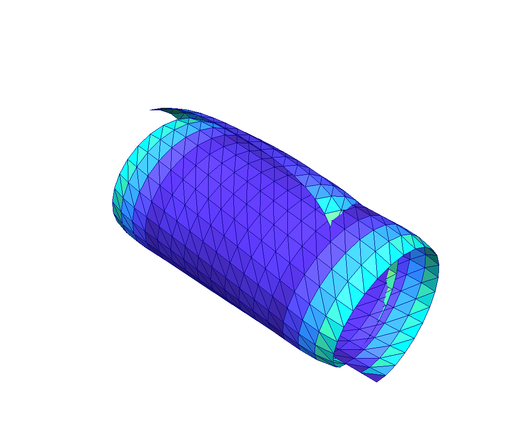
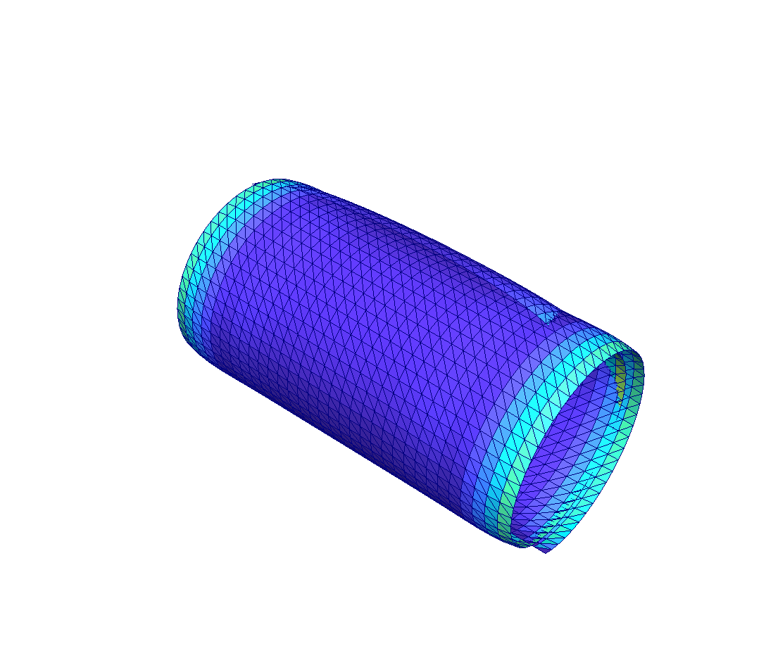
hold at all nodes . The employed finite element spaces are depicted in Figure 5.
Crucial for the finite element discretization of the bending problem is the definition of a discrete gradient operator
which allows us to define discrete second order derivatives of functions via
Here we make use of the fact that . The discrete gradient operator is for given defined as the unique piecewise quadratic, continuous vector field that satisfies the condition
for all while the degrees of freedom associated with the sides of elements are defined by the two conditions
for all sides with normals , tangent vectors , and midpoints . For , we set
With the discrete second derivatives we are in a position to state the finite element discretization of the plate bending model:
To prove the correctness of this discretization we show that existing finite element minimizers accumulate at admissible isometries, incorporate that the bending energy is weakly lower semicontinuous, and use that isometries can be approximated by smooth isometries which is a result proved in [47, 40].
Theorem 3.3 (Convergent approximation).
For every there exists a minimizer . If is a sequence of almost-minimizers, then , for all , and every accumulation point of the sequence is a strong accumulation point, belongs to the continuous admissible set and is minimal for .
Proof (sketched).
We follow the typical steps for establishing a -convergence result
provided in [7, 10].
(a) Using the boundary conditions included in the set it follows
that the mapping is a norm on the subset of
with functions satisfying corresponding homogeneous
boundary conditions. This leads to a coercivity property and the existence
of discrete solutions.
(b) The uniform discrete coercivity property implies that the sequences
and have weak accumulation points and
in
which are compatible in the sense that . Moreover, we have
that and weak lower semicontinuity of the norm shows that
(c) Let be a minimizer for . The continuity of the functional with respect to the strong topology in in combination with the density results for smooth isometries established in [40] allow us to assume that is smooth. We may thus define an approximating sequence of finite element functions by setting . Approximation properties of the interpolation operator lead to the inequality
which proves the statement. ∎
4. Iterative solution via constrained gradient flows
The practical solution of the finite element discretizations of the nonlinear bending problems is nontrivial due to the presence of nonlinear pointwise constraints and the corresponding lack of higher regularity properties. To provide a reliable strategy that decreases the energy we adopt gradient flow strategies. Our estimates show that these converge to stationary, low energy configurations. We will always use a linearized treatment of the constraints which is then discretized semi-implicitly. This makes the iterative scheme practical. To illustrate the main idea, consider the following abstract minimization problem in a Hilbert space :
| () |
Here, we assume that the constraint is understood pointwise with a function . The Euler–Lagrange equations for the problem are then formally given by the identity
for all with a Lagrange multiplier . Note that the term involving disappears if satisfies and that this is sufficient to characterize a stationary point subject to the constraint. The corresponding gradient flow is formally defined via
Our corresponding time-stepping scheme uses the backward difference quotient operator for a step-size and determines iterates via the linearly constrained problems
We specify the meaning of the iterative scheme in the following algorithm.
Algorithm 4.1 (Abstract constrained gradient descent).
Let be such that and and choose ,
set .
(1) Compute such that
for all under the constraints , i.e.,
(2) Stop the iteration if ; otherwise increase and continue with (1).
We remark that it is useful to regard rather than as the unknown in the iteration steps. In particular, we may eliminate via the identity with the known function . A geometric interpretation of the iteration is that given an iterate the correction is computed in the tangent space of the level set of defined by the value . Note that we do not use a projection step onto the zero level set of since this will in general not be energy stable. Figure 6 illustrates the conceptual idea of Algorithm 4.1.
The following theorem states the main features of Algorithm 4.1, i.e., its unconditional energy stability with the resulting convergence to a stationary configuration of lower energy and the control of the constraint violation by the step size.
Theorem 4.2 (Convergent iteration).
Assume that is convex, coercive, continuous, and Fréchet differentiable on and is twice differentiable with uniformly bounded second derivative, i.e., we have for all . Then, the iterates of Algorithm 4.1 are uniquely defined and satisfy for the energy estimate
Moreover, if is a norm on with the property for all then we have the constraint violation bound
where . In particular, we have that and Algorithm 4.1 terminates within a finite number of iterations. The output satisfies the residual estimate
Proof.
(a) The existence of the iterates follows by applying the direct method of the calculus of variations to the minimization problems:
The solution is unique and the corresponding Euler–Lagrange equation
coincides with the equation that defines the iterates in
Algorithm 4.1.
(b) Choosing the admissible test function and using the
convexity of leads to
A multiplication by and summation over prove
the energy stability.
(c) With a Taylor expansion of about the iterate and
the imposed identity we find that
Repeating this argument and noting that leads to the estimate
Applying the norm to the estimate, using the triangle
inequality, and incorporating the assumed
bound as well as the energy bound
proves the estimate for the constraint violation error.
(d) The estimate for is an immediate consequence of
the bound .
∎
Examples of pairs of norms and that satisfy the assumed estimate are the norm in combination with the norm or the norm together with a Sobolev norm in with sufficiently large. It is remarkable that the violation of the constraint is independent of the number of iterations. An explanation for this is that the updates converge quickly to zero in the gradient flow iteration.
4.1. Elastic rods
We apply the abstract framework for constrained minimization problems to the energy functional describing the bending-torsion behavior of elastic rods. For a vector field we set
while for a vector field we define
The functionals and are the components of corresponding to the variables and , respectively. We generate a sequence that approximates a stationary configuration for with the following algorithm.
Algorithm 4.3 (Gradient descent for elastic rods).
Choose an initial pair and a step size ,
set .
(1) Compute such that for all we have
(2) Compute such that for all we have
(3) Stop the iteration if
otherwise, increase and continue with (1).
Again, it is useful to view and as the unknowns in Steps (1) and (2) instead of and . The algorithm exploits the fact that the penalty term is separately convex while the nonquadratic contribution to the torsion term is separately concave. Therefore, the decoupled semi-implicit treatment of these terms is natural and unconditionally energy stable.
Proposition 4.4 (Convergent iteration).
Assume that we have
for all with . Algorithm 4.3 is well defined and produces a sequence such that for all we have
The iteration controls the unit-length violation via
where . In particular, the algorithm terminates within a finite number of iterations.
Proof.
(a) To prove the stability estimate we note that the functional
is separately convex, i.e., convex in and in . Therefore, we have that
which by summation leads to the inequality
Similarly, the functional
is separately convex and we have
By choosing and in the equations of Steps (2) and (3) of Algorithm 4.3 we thus find that
Since
we deduce the asserted estimate.
(b) The nodal orthogonality conditions encoded in the spaces
and lead to the relations
By induction and incorporation of the stability estimate we deduce the asserted estimates for the constraint violation. ∎
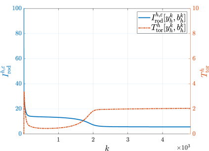
We illustrate the performance of Algorithm 4.3 via a numerical experiment showing the relaxation of a twisted initially flat curve which is clamped at both ends. We plotted in the bottom of Figure 7 the total energy and the torsion contribution defined by
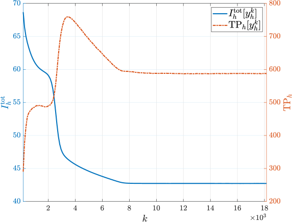
We observe that the curve quickly releases its large energy and becomes a spatial curve attaining a stationary configuration with equilibrated curvature after approximately 2000 iterations. The model parameters used in the simulation were set to and . We used a partition into 1006 subintervals corresponding to a mesh-size . The step-size and the penalty parameter were chosen proportional to .


4.2. Elastic plates
We next apply the conceptual approach for solving nonlinearly constrained minimization problems outlined above to the case of approximating bending isometries. For this we recall that the discrete bending energy is given by
with the set of admissible discrete deformations defined as
Using the linearized isometry operator
we define the (shifted) tangent space of the set of discrete isometric deformations at a deformation via
We then decrease the bending energy for given boundary conditions by iterating the steps of the following algorithm.
Algorithm 4.5 (Gradient descent for elastic plates).
Choose an initial and a step size , set .
(1) Compute such that
for all we have
(2) Stop if ; otherwise, increase and continue with (1).
The iterates will in general not satisfy the nodal isometry constraint exactly, but the violation is again independent of the number of iterations and controlled by the step size .
Proposition 4.6 (Convergent iteration).
The iterates of Algorithm 4.5 are well defined and satisfy for every the energy estimate
Moreover, if for all with , then we have the constraint violation bound
where .
Proof (sketched).
(a) Since for any we have that
is a nonempty linear space the Lax-Milgram lemma implies that
there exists a unique solution .
(b) The energy decay property is an immediate consequence of choosing
and using the binomial formula
(c) The error bound for the isometry violation follows from the orthogonality defined by the linearized isometry condition and the energy decay property as in the proof of Proposition 4.2. ∎
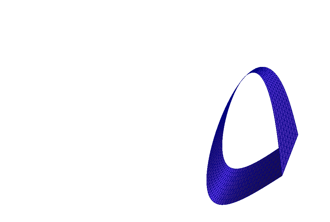
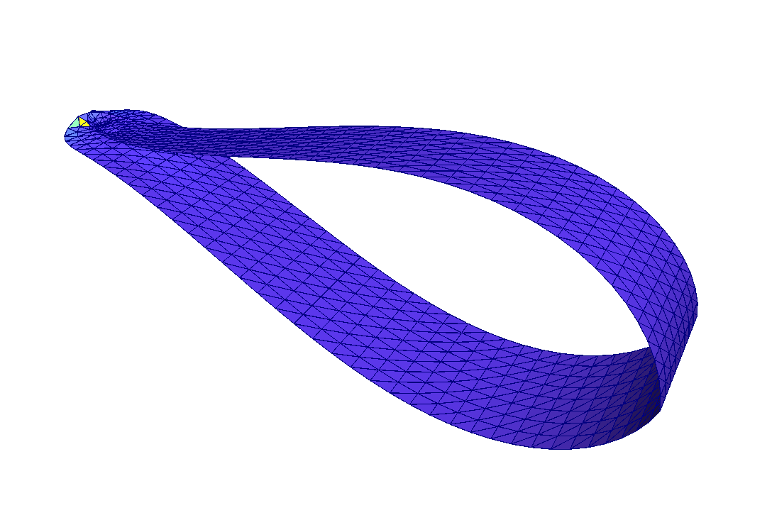
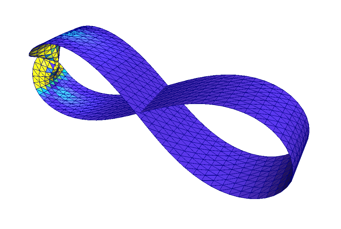
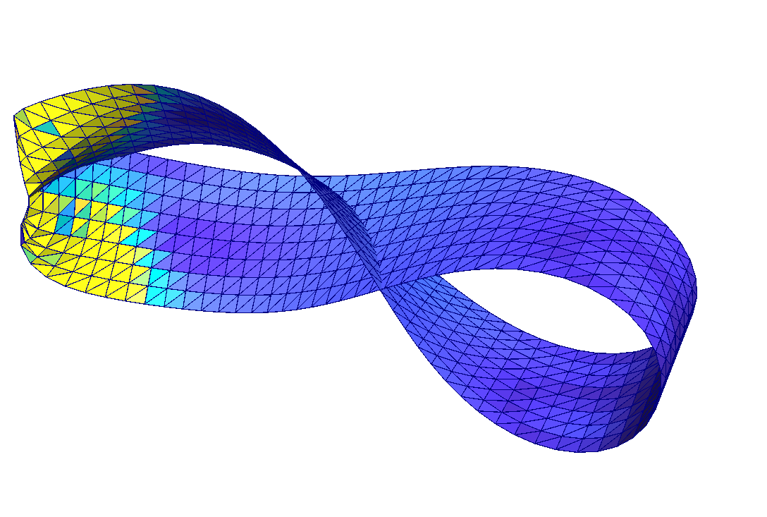
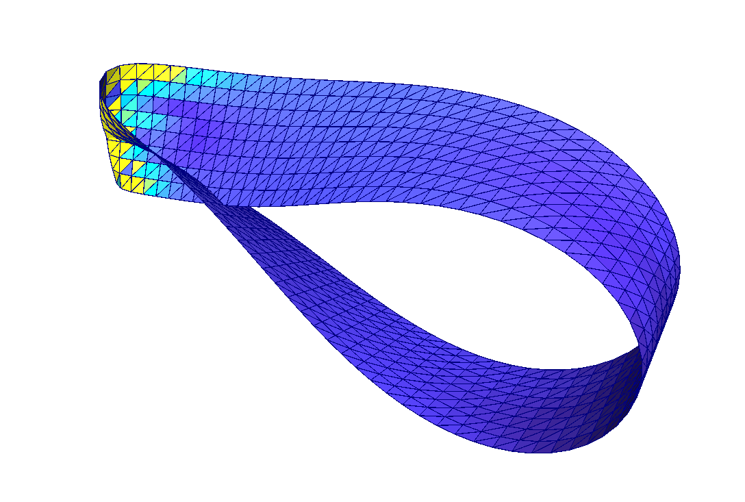
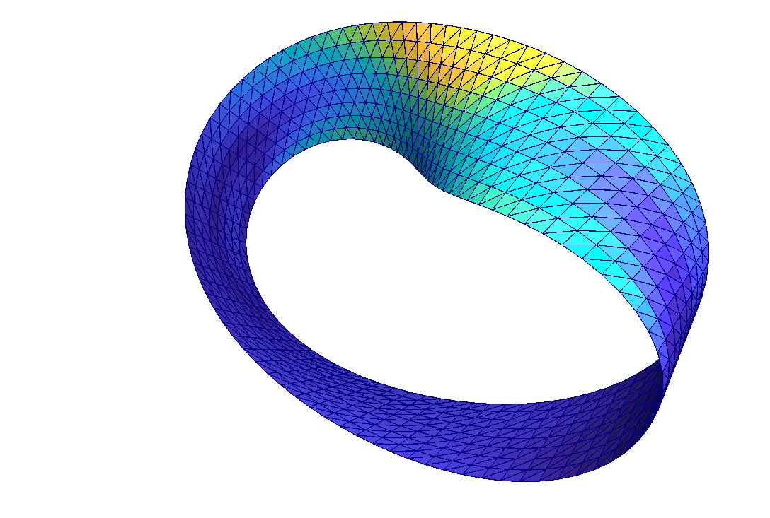
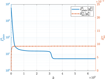
Figure 8 illustrates the discrete evolution defined by Algorithm 4.5 via snapshots of different iterates. The clamped boundary conditions imposed at the ends of the strip with length and width are defined via the operator
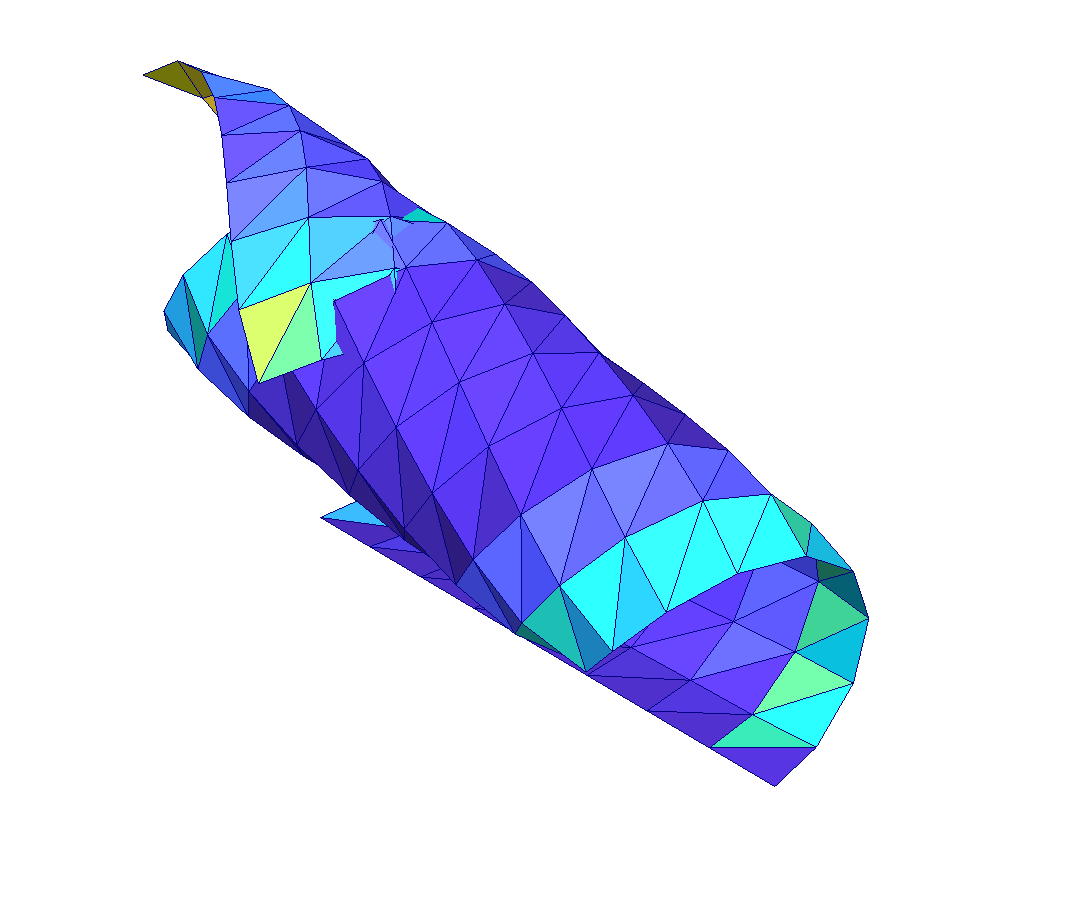
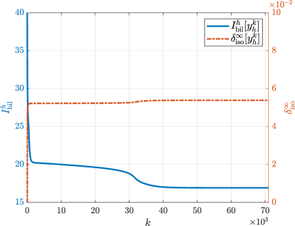
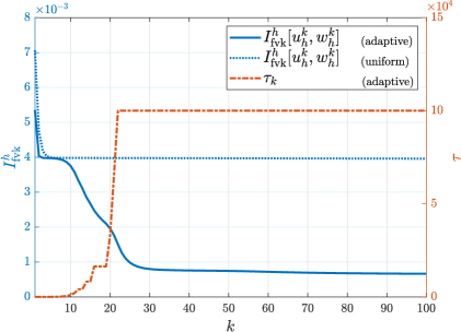
and functions and . These functions are constructed in such a way that the segment is rotated and mapped onto the fixed opposite segment . In this way the formation of a Möbius strip is enforced, we included a small linear forcing term to avoid certain nonuniqueness effects. We observe that the nonsmooth choice of the starting value with large bending energy does not influence the robustness of the iteration and that within less than iterations a stationary configuration for the stopping parameter and evolution metric with is attained. We also observe that we obtain a satisfactory stationary shape for coarse triangulations and that the energy decreases monotonically as predicted, with a small violation of the isometry constraint indicated by the quantity
which appears to be nearly independent of the iteration. We finally remark that we observe concentrations of curvature at boundary points corresponding to certain singularities discussed in [15].


5. Linear finite element systems with nodal constraints
The discrete gradient flows devised in the previous sections lead to linear systems of equations in the time steps that have a special saddle point structure. In particular, they are given in the form
| () |
with a fixed positive definite symmetric matrix and a matrix that changes in the iteration steps. The matrix is of full rank and block diagonal, i.e.,
with vectors for and . We note that the solution of the linear system of equations above is equivalently characterized by the system
for all belonging to the kernel of , i.e., subject to the conditions
To obtain a simpler, unconstrained system of equations we choose for each a set of orthonormal vectors that are orthogonal to , i.e., we have
We may then represent the kernel of by the image of the matrix defined by
The matrix defines an isomorphism and we may thus reformulate the linear system of equations as
| () |
With the solution we obtain the solution of the orginal system () via . Since the columns of are linearly independent the matrix has full rank. Hence, the symmetric matrix is positive definite and the linear system of equations can be solved efficiently with a preconditioned conjugate gradient scheme. The construction of suitable preconditioners has been discussed in [45] and the main issue in their justification is to understand how accurate the approximation
is. Straightforward manipulations show that the solution of the saddle-point system () satisfies
With the equvialent formulation and we find that
Since is orthogonal in the sense that it follows that
This justifies the approximation if the second term on the right-hand side is small. Another relation is obtained by formally applying the Neumann series
to the product with a suitable parameter to deduce that
Accepting the approximation the next step is to choose a preconditioner for , i.e., approximates and the multiplication by is inexpensive, and use the matrix as a preconditioner for . Noting that is orthogonal this is justified by the spectral norm estimate from [45],
A further discussion of related preconditioners in the context of micromagnetics can be found in [41]. We illustrate the construction of the bases of the null space and the performance of different solution strategies in the context of harmonic maps into spheres.
5.1. Application to harmonic maps
Harmonic maps are vector fields with values in a given manifold which are stationary for the Dirichlet energy. In the case of the unit sphere, the vector field satisfies a pointwise unit-length constraint. Already this simple case illustrates analytical difficulties when dealing with constrained partial differential equations. In particular, harmonic maps are nonunique even for fixed boundary values and may be discontinuous everywhere, cf. [50]. Partial regularity results can be proved if a harmonic map is energy minimizing, cf. [56]. These observations underline the importance of computing harmonic maps with low energy. We aim at applying the concepts of the previous sections to the approximation of harmonic maps and consider the following model problem defined with a function with for all which is the trace of a function :
Following [1, 6] we discretize the admissible set by piecewise affine vector fields and impose the unit-length constraint in the nodes of the underlying triangulation. This leads to the following discrete minimization problem:
For a function with nonvanishing nodal values we define
With a gradient flow approach and a linearized treatment of the nodal constraint we are led to the following algorithm.
Algorithm 5.1 (Gradient descent for harmonic maps).
Choose and , set .
(1) Compute such that for all
we have
(2) Stop if ; otherwise, increase and continue with (1).
The Lax–Milgram lemma shows that the iteration is well defined. Because of the orthogonality condition we have that
which by induction gives for . If the restriction of the inner product to is represented by the matrix then the linear systems in the iteration can be written as
with the vectorial finite element element stiffness matrix and the constraint matrix
To define the matrix that provides an isomorphism from onto the kernel of we need to compute for a given vector an orthonormal basis of its orthogonal complement. We proceed as follows: if is parallel to then we choose the remaining canonical basis vectors ; otherwise, we set
where denotes the rotation of by , followed by the normalization for .
Example 5.2.
Let and define on for via
The employed triangulations result from uniform refinements of a reference triangulation of into six tetrahedra. The starting value is defined by generating random nodal values of unit length.
Table 2 compares the following general strategies to solve the linear problems in the iterative solution of harmonic maps:
- (1)
- (2)
- (3)
- (4)
We measured the average time needed for different discretizations to solve the linear systems of equations using strategies (1)-(4). We always chose the step size , the stopping parameter for the relative residuals in the preconditioned conjugate gradient scheme, and the stopping criterion in Algorithm 5.1. We employed the inner product to define and used Matlab’s backslash operator as a model direct solver for sparse linear systems. From the obtained numbers we see that the preconditioner particularly designed for the structure of the constrained problems with changing constraints clearly outperforms all other approaches. However, it does not lead to mesh-size independent iteration numbers for this example with a nonsmooth solution. We also remark that we did not observe a further improvement when additional terms in the Neumann series were used with a damping factor . In a two-dimensional setting with a smooth solution the complete Cholesky factorization led to mesh-independent iteration numbers.
| saddle, direct | reduced, direct | reduced, pcg | reduced, pcg | |
| (backslash) | (backslash) | (diagonal ) | (incompl. Chol.) | |
| (11.9) | (6.0) | |||
| (25.4) | (10.2) | |||
| (52.5) | (19.9) | |||
| (105.9) | (38.8) | |||
| – | – | (212.1) | (76.1) |
6. Applications, modifications, and extensions
We address in this section the application of the developed methods to the simulation of extended problems. In particular, we devise a numerical method for simulating bilayer plates, discuss how injectivity can be enforced in the case of elastic rods, and investigate a model that involves the thickness parameter and thereby allows for describing situations in which low energy membrane and bending effects occur simultaneously.
6.1. Bilayer plates
An important class of applications of nonlinear plate bending is related to composite materials, i.e., structures such as bilayer plates which are made of two sheets with slightly different mechanical features that are glued on top of each other. The difference in the material properties, e.g., concerning the response to environmental changes such as temperature, allows for externally controlled large bending effects. In bimetal strips one of the metals contracts while the other one expands leading in combination to the formation of rolls with prescribed curvature.
The preferred curvature is defined by the difference in elastic properties of the involed materials and is explicitly visible in the dimensionally reduced model identified in [53]. Following that work we consider a thin plate and the inhomogeneous energy density
with a material parameter . The energy density is assumed to satisfy the standard requirements stated in Section 2 so that is minimal for deformation gradients which are multiples of rotations with if and for corresponding to expansive and contractive behavior in the upper and lower sheets, respectively. It has been shown in [53] that for deformations with energy proportional to a limiting, dimensionally reduced problem is given by the following minimization problem:
Here, is the reduced quadratic form introduced in Section 2.2 which is applied to the difference of the second fundamental form and a multiple of the identity matrix with a factor given by half of the jump in the material difference divided by . This material mismatch introduces a term that is similar to so-called spontaneous curvature terms in the context of biomembranes described via the Helfrich-Willmore model. Note that in the definition of the difference is and its proportionality to the thickness of the plates is important to avoid delamination effects. The reduced model prefers deformations that define surfaces with mean curvature and vanishing Gaussian curvature due to the isometry constraint. Hence, rolling effects in one direction occur. In [54] global minimizers for have been shown to be given by cylinders with radius . Recalling that the quadratic form is given by the scalar product
we do not have the property that the integrand is proportional to as in the case of a single layer or two identical materials corresponding to the case . Instead we infer
Because of the isometry condition the first term is proportional to while the third term is a constant which is irrelevant for the minimization process. For the second term on the right-hand side we have
Therefore, using we have
Convergent finite element discretizations and iterative strategies for the numerical solution of the bilayer plate bending problem have been devised in the articles [14, 13] extending the ideas described in the Sections 3.2 and 4.2. The iterative scheme of [14] is unconditionally stable but requires a subiteration, i.e., the solution of a nonlinear system of equations in every time step, which limits its practical applicability, while the scheme used in [13] is explicit and efficient but can only be expected to be conditionally stable. We devise here a new semi-implicit scheme with improved stability properties. The set of admissible deformations and the tangent spaces are defined as in Section 3.2 and we set
for a function with a componentwise application in the case of a vector field. The discretized energy functional describing actuated bilayer plates is therefore given by
A uniform discrete coercivity property of this discretization has been established in [14]. The new iterative minimization from [16] uses an explicit treatment of the spontaneous curvature term.
Algorithm 6.1 (Gradient descent for bilayer plates).
Choose and , set .
(1) Compute such that for all we have
(2) Stop if ; otherwise increase and continue with (1).
We show that the iteration of Algorithm 6.1 is energy stable on finite time intervals under a moderate condition on the step-size resulting from the use of an inverse estimate. To formulate it, we first note that we assume that the boundary conditions imply a Poincaré type estimate
for all with . With this estimate one verifies that the mesh-dependent estimate
holds for all with and with the minimal mesh-size .
Proposition 6.2 (Convergent iteration).
The iterates of Algorithm 6.1 are well defined. Assume that we have
for all with . Then there exist constants such that if for we have
and
where .
Proof.
We argue by induction and assume that the estimate has been established for . Choosing and using Hölder’s inequality shows that for we have
Absorbing terms involving on the left-hand side and noting that terms involving are bounded because of the bounds for , we find that
Here, we also used that the discrete energy is coercive. With this intermediate estimate and the orthogonality condition encoded in the definition of we infer with that
and hence with the inverse estimate we obtain the suboptimal estimate that
To obtain the energy bound we note that a discrete product rule shows that the discrete time derivative of the spontaneous curvature term is given by
Comparing this expression with the right-hand side of the equation in Step (1) of Algorithm 6.1 with leads to
We use the estimates and for and , to bound the right-hand side by . This leads to
and proves the asserted energy estimate. With this bound we also obtain the improved bound for the constraint violation error. ∎
The good stability properties of the newly proposed numerical scheme are confirmed by a numerical experiment whose outcome is visualized in Figure 10. The setup uses a rectangular strip of length and width that is clamped at one end. The spontaneous curvature parameter is and we have and . The figure shows snapshots of the evolution on a grid with medium mesh-size and stationary states for different triangulations with mesh-sizes proportional to , . The step-size was always set to . The stopping criterion was chosen as . Because of the extreme geometry and the large deformation the asymmetry of the underlying triangulations is reflected in the numerical solutions but this effect disappears for smaller mesh-sizes. The theoeretical results about the energy monotonicity and controlled constraint violation are confirmed by the bottom plot of Figure 10.


6.2. Selfavoiding curves and elastic knots
A strategy for finding useful representatives of knot classes, i.e., closed curves within a given isotopy class with particular features, is to minimize or decrease the bending energy within the given class via continuous evolutions defined by a gradient flow. To ensure that the flow does not change the topological properties of the curve, appropriate terms have to be included in the mathematical formulation. To this end we add a self-avoidance potential to the bending energy that prevents the curve from self-intersecting or pulling tight, i.e., we consider flows determined by functionals
in sets of curves satisfying periodic or, e.g., clamped boundary conditions. We refer the reader to [46] for a general discussion of appropriate functionals. A functional that turned out to have several advantageous features is the tangent-point functional proposed in [39]. It is for a curve defined via the tangent-point radius which is the radius of the circle that is tangent to in and intersects the curve in the point . For curves that are parametrized by arclength we have
which follows from investigating the geometrical configuration sketched in Figure 11. If then we have that converges to the inverse of the curvature of the curve at . If otherwise for fixed then the radius converges to zero as depicted in Figure 12. An alternative choice is the use of the Menger curvature which is discussed in [59].
The tangent-point functional is for an exponent defined via
The exponent has to be suitably chosen so that singularities corresponding to a vanishing tangent-point radius are sufficiently strong to lead to an infinite value of the functional. Thereby, an energy barrier is defined that separates different isotopy classes. The functional has important and remarkable features.
Remarks 6.3.
(i) If the arclength-parametrized curve is injective
then is finite if and only if ,
cf. [22].
(ii) For all and there exists a constant such that
for all arclength-parametrized curves with
we have the bi-Lipschitz estimate for all ,
cf. [23].
In particular, is a knot energy in the sense that for a family
of curves converging pointwise to a curve with self-intersection,
the values blow up, cf. [63, 46, 60, 23].
(iii) The functional is twice continuously differentiable with bounded
variations and integrands, cf. [23, 17].
To decrease the total energy of a given initial curve within its isotopy class we use a discretization of the evolution
subject to the linearized arclength conditions and . The discretization uses the ideas outlined in Sections 3.1 and 4.1 with an explicit treatment of the potential.
Algorithm 6.4 (Gradient descent for selfavoiding curves).
Choose an initial and a step-size ,
set .
(1) Compute such that for all
we have
(2) Stop the iteration if ; otherwise, increase and continue with (1).
The explicit treatment of the potential has several advantages. First, we obtain linear problems in the time steps. Second, we avoid the inversion of fully populated matrices. Third, the assembly of the vector on the right-hand side can be fully parallelized without communication costs. Finally, we do not change the stability of the iteration compared to a fully implicit time stepping scheme since the potential does not have obvious convexity properties. Using the differentiability properties of the functional and assuming that the flow metric is the scalar product, it has been shown in [17] that the conditional energy decay property
holds for all with a finite time horizon . This inequality implies the convergence of the iteration to a stationary configuration. Since the total energy is bounded uniformly, the values of the potential remain controlled so that in case of a sufficient resolution no self-contact or topology changes can occur.
The good stability properties and corresponding selfavoidance behavior of the numerical scheme are illustrated by the snapshots of configurations and the corresponding energy decay shown for a generic setting in Figure 13. We observe that the curve relaxes to a curve with equilibrated curvature and which is nearly flat. While the total energy decreases the (unscaled) tangent-point functional increases. In the experiments we used the model parameters , , . The initial curve belongs to the knot class , cf. [51], and has a total length which is accurately preserved during the evolution. To compute the evolution we used a partitioning of the reference interval into subintervals. The step-size was chosen proportional to the mesh-size .


6.3. Föppl–von Kármán model
The nonlinear bending model discussed in the previous sections is not suitable to describe certain phenomena such as the formation of wrinkles which occur for very small energies. In order to describe these effects in a dimensionally reduced model it is essential to involve the thickness parameter as this number determines the oscillating or nonsmooth behavior of deformations. A model that captures such effects is the Föppl–von Kármán model which can be identified via different scalings of the in-plane and out-of-plane components of a three-dimensional deformation when is small. It determines a planar displacement and a deflection as a minimizing pair for the energy functional
in a set of admissible pairs contained in the product space . Here, we use the symmetric gradient
and the dyadic product
where is understood as a column vector. We refer the reader to [26, 27, 35, 37] for justifications of this minimization problem as a simplification of three-dimensional hyperelastic material models. It has been shown rigorously in [44, 62] that the presence of the parameter leads to minimizers with wrinkling patterns whose geometry is determined by the parameter . This is done by identifying optimal scaling laws of the energy in terms of , cf. [20, 30] for further examples. Only a few numerical methods for minimizing the Föppl–von Kármán energy are available, cf. [28] for an abstract investigation.
To minimize the energy for given boundary conditions we follow [12] and again adopt a gradient flow appraoch defined by the system
Here, and are inner products on and , respectively, and we used the identities and for a symmetric matrix and . The temporal discretization of the system decouples the equations via a semi-implicit evaluation of different terms. In particular, given we compute such that
for all satisfying appropriate homogeneous boundary conditions. The average is defined for subsequent approximations and via
The unconditional stability and energy decay of the iteration follows from choosing and and exploiting a discrete product rule, cf. [12] for details. The problems in the time steps determine minimizers of certain functionals and if then these functionals are strongly convex and minimizers are uniquely defined. Correspondingly, we expect the Newton scheme to converge provided that the step-size is sufficiently small.
For a full discretization we use the set of admissible pairs
and the corresponding homogeneous space
To avoid an unnecessary small uniform step-size we instead use variable step-sizes that are adjusted according to the performance of the Newton scheme using the following rules:
The parameter defines an upper bound for the step-sizes and avoids a numerical overflow. The ideas lead to the following algorithm.
Algorithm 6.5 (Gradient descent for Föppl–von Kármán functional).
Choose , an integer ,
stopping tolerances ,
and an initial step-size , set .
(1a) Repeatedly decrease until the Newton scheme terminates within steps
and tolerance to determine such that
for all .
(1b) Compute such that
for all .
(2) Stop if ;
otherwise, define
increase , and continue with (1).
Note that in the algorithm a stopping criterion is used that is proportional to the step-size which is important in the case of small step-sizes. To illustrate the performance of the algorithm and features of the mathematical model we follow [12] and consider the compression of a plate along one of its sides. Particularly, we let and compress the side by 10 percent which defines the boundary data for the in-plane displacement . We use homogeneous clamped boundary conditions along the same side for the deflection . The results shown in Figure 14 confirm the formation of wrinkling structures. These depend on both the numerical resolution and the thickness parameter. Moreover, the energy decay shown in the bottom plot of Figure 14 indicates that these are only obtained within a reasonable number of iterations if an adaptive step-size strategy is used.


7. Conclusions
We have addressed in this article the accurate finite element discretization and reliable iterative solution of nonlinear models for describing large deformations of elastic rods and plates. To avoid unjustified regularity assumptions we have adopted the concept of -convergence and thereby proved convergence of approximations. To compute stationary configurations of low and possibly minimal energy we have used gradient flow discretizations that are guaranteed to decrease the elastic energy and preserve inextensibility and isometry constraints appropriately. These two concepts leave a theoretical gap in the sense that the framework of -convergence is concerned with global energy minimizers while gradient flows can only be expected to determine stationary configurations. However, -convergence goes beyond global energy minimization and gradient flows typically avoid unstable critical configurations. These properties are convincingly confirmed by our numerical experiments which did not employ any a priori knowledge about expected solutions. The state of the art of reliable methods for computing nonlinear bending phenomena leaves open several aspects such as the development of optimal preconditioners, adaptive refinement of stress concentrations, determination of convergence rates, effective combination with membrane effects, or simulation of realistic dynamic models open. We believe that the methods presented in this article can be useful in investigating them in future research.
Acknowledgments. The author wishes to thank his coworkers in various collaborations that led to the results presented in this article.
References
- [1] F. Alouges. A new algorithm for computing liquid crystal stable configurations: the harmonic mapping case. SIAM J. Numer. Anal., 34(5):1708–1726, 1997.
- [2] S. S. Antman. Nonlinear problems of elasticity, volume 107 of Applied Mathematical Sciences. Springer, New York, second edition, 2005.
- [3] B. Audoly and Y. Pomeau. Elasticity and geometry. Oxford University Press, Oxford, 2010.
- [4] J. W. Barrett, H. Garcke, and R. Nürnberg. A parametric finite element method for fourth order geometric evolution equations. J. Comput. Phys., 222(1):441–462, 2007.
- [5] J. W. Barrett, H. Garcke, and R. Nürnberg. Parametric approximation of isotropic and anisotropic elastic flow for closed and open curves. Numer. Math., 120(3):489–542, 2012.
- [6] S. Bartels. Stability and convergence of finite-element approximation schemes for harmonic maps. SIAM J. Numer. Anal., 43(1):220–238, 2005.
- [7] S. Bartels. Approximation of large bending isometries with discrete Kirchhoff triangles. SIAM J. Numer. Anal., 51(1):516–525, 2013.
- [8] S. Bartels. Finite element approximation of large bending isometries. Numer. Math., 124(3):415–440, 2013.
- [9] S. Bartels. A simple scheme for the approximation of the elastic flow of inextensible curves. IMA J. Numer. Anal., 33(4):1115–1125, 2013.
- [10] S. Bartels. Numerical methods for nonlinear partial differential equations, volume 47 of Springer Series in Computational Mathematics. Springer, Cham, 2015.
- [11] S. Bartels. Projection-free approximation of geometrically constrained partial differential equations. Math. Comp., 85(299):1033–1049, 2016.
- [12] S. Bartels. Numerical solution of a Föppl–von Kármán model. SIAM J. Numer. Anal., 55(3):1505–1524, 2017.
- [13] S. Bartels, A. Bonito, A. H. Muliana, and R. H. Nochetto. Modeling and simulation of thermally actuated bilayer plates. J. Comput. Phys., 354:512–528, 2018.
- [14] S. Bartels, A. Bonito, and R. H. Nochetto. Bilayer plates: model reduction, -convergent finite element approximation, and discrete gradient flow. Comm. Pure Appl. Math., 70(3):547–589, 2017.
- [15] S. Bartels and P. Hornung. Bending paper and the Möbius strip. J. Elasticity, 119(1-2):113–136, 2015.
- [16] S. Bartels and C. Palus. Stable iterative solution of bilayer bending problems. (In preparation), 2019.
- [17] S. Bartels and P. Reiter. Stability of a simple scheme for the approximation of elastic knots and self-avoiding inextensible curves. arXiv, (arXiv:1804.02206), 2018.
- [18] S. Bartels and P. Reiter. Numerical solution of a bending-torsion model for elastic rods. (In preparation), 2019.
- [19] S. Bartels, P. Reiter, and J. Riege. A simple scheme for the approximation of self-avoiding inextensible curves. IMA J. Numer. Anal., 38(2):543–565, 2018.
- [20] P. Bella and R. V. Kohn. Metric-induced wrinkling of a thin elastic sheet. J. Nonlinear Sci., 24(6):1147–1176, 2014.
- [21] M. Bergou, M. Wardetzky, S. Robinson, B. Audoly, and E. Grinspun. Discrete Elastic Rods. ACM Transactions on Graphics (SIGGRAPH), 27(3):63:1–63:12, aug 2008.
- [22] S. Blatt. The energy spaces of the tangent point energies. J. Topol. Anal., 5(3):261–270, 2013.
- [23] S. Blatt and P. Reiter. Regularity theory for tangent-point energies: the non-degenerate sub-critical case. Adv. Calc. Var., 8(2):93–116, 2015.
- [24] A. Bonito, R. H. Nochetto, and D. Ntogkas. DG approach to large bending plate deformations with isometry constraint. (In preparation), 2019.
- [25] D. Braess. Finite elements. Cambridge University Press, Cambridge, third edition, 2007.
- [26] P. G. Ciarlet. A justification of the von Kármán equations. Arch. Rational Mech. Anal., 73(4):349–389, 1980.
- [27] P. G. Ciarlet. Mathematical elasticity. Vol. II, volume 27 of Studies in Mathematics and its Applications. North-Holland Publishing Co., Amsterdam, 1997. Theory of plates.
- [28] P. G. Ciarlet, L. Gratie, and S. Kesavan. Numerical analysis of the generalized von Kármán equations. C. R. Math. Acad. Sci. Paris, 341(11):695–699, 2005.
- [29] S. Conti and F. Maggi. Confining thin elastic sheets and folding paper. Arch. Ration. Mech. Anal., 187(1):1–48, 2008.
- [30] S. Conti, H. Olbermann, and I. Tobasco. Symmetry breaking in indented elastic cones. Math. Models Methods Appl. Sci., 27(2):291–321, 2017.
- [31] G. Dal Maso. An introduction to -convergence, volume 8 of Progress in Nonlinear Differential Equations and their Applications. Birkhäuser Boston, Inc., Boston, MA, 1993.
- [32] K. Deckelnick, G. Dziuk, and C. M. Elliott. Computation of geometric partial differential equations and mean curvature flow. Acta Numer., 14:139–232, 2005.
- [33] G. Dziuk, E. Kuwert, and R. Schätzle. Evolution of elastic curves in : existence and computation. SIAM J. Math. Anal., 33(5):1228–1245, 2002.
- [34] L. Freddi, P. Hornung, M. G. Mora, and R. Paroni. A corrected Sadowsky functional for inextensible elastic ribbons. J. Elasticity, 123(2):125–136, 2016.
- [35] G. Friesecke, R. D. James, and S. Müller. The Föppl-von Kármán plate theory as a low energy -limit of nonlinear elasticity. C. R. Math. Acad. Sci. Paris, 335(2):201–206, 2002.
- [36] G. Friesecke, R. D. James, and S. Müller. A theorem on geometric rigidity and the derivation of nonlinear plate theory from three-dimensional elasticity. Comm. Pure Appl. Math., 55(11):1461–1506, 2002.
- [37] G. Friesecke, R. D. James, and S. Müller. A hierarchy of plate models derived from nonlinear elasticity by gamma-convergence. Arch. Ration. Mech. Anal., 180(2):183–236, 2006.
- [38] G. Friesecke, S. Müller, and R. D. James. Rigorous derivation of nonlinear plate theory and geometric rigidity. C. R. Math. Acad. Sci. Paris, 334(2):173–178, 2002.
- [39] O. Gonzalez and J. H. Maddocks. Global curvature, thickness, and the ideal shapes of knots. Proc. Natl. Acad. Sci. USA, 96(9):4769–4773, 1999.
- [40] P. Hornung. Approximation of flat isometric immersions by smooth ones. Arch. Ration. Mech. Anal., 199(3):1015–1067, 2011.
- [41] J. Kraus, C.-M. Pfeiler, D. Praetorius, M. Ruggeri, and B. Stiftner. Iterative solution and preconditioning for the tangent plane scheme in computational micromagnetics. arXiv, (1808.10281), 2018.
- [42] J. Langer and D. A. Singer. Lagrangian aspects of the Kirchhoff elastic rod. SIAM Rev., 38(4):605–618, 1996.
- [43] M. G. Mora and S. Müller. Derivation of the nonlinear bending-torsion theory for inextensible rods by -convergence. Calc. Var. Partial Differential Equations, 18(3):287–305, 2003.
- [44] S. Müller and H. Olbermann. Almost conical deformations of thin sheets with rotational symmetry. SIAM J. Math. Anal., 46(1):25–44, 2014.
- [45] S. G. Nash and A. Sofer. Preconditioning reduced matrices. SIAM J. Matrix Anal. Appl., 17(1):47–68, 1996.
- [46] J. O’Hara. Energy of knots and conformal geometry. volume 33 of Series on Knots and Everything, pages xiv+288. World Scientific Publishing Co., Inc., River Edge, NJ, 2003.
- [47] M. R. Pakzad. On the Sobolev space of isometric immersions. J. Differential Geom., 66(1):47–69, 2004.
- [48] O. Pantz. On the justification of the nonlinear inextensional plate model. Arch. Ration. Mech. Anal., 167(3):179–209, 2003.
- [49] P. Pozzi and B. Stinner. Curve shortening flow coupled to lateral diffusion. Numer. Math., 135(4):1171–1205, 2017.
- [50] T. Rivière. Everywhere discontinuous harmonic maps into spheres. Acta Math., 175(2):197–226, 1995.
- [51] D. Rolfsen. Knots and links, volume 7 of Mathematics Lecture Series. Publish or Perish, Inc., Houston, TX, 1990. Corrected reprint of the 1976 original.
- [52] O. Sander, P. Neff, and M. Bîrsan. Numerical treatment of a geometrically nonlinear planar Cosserat shell model. Comput. Mech., 57(5):817–841, 2016.
- [53] B. Schmidt. Minimal energy configurations of strained multi-layers. Calc. Var. Partial Differential Equations, 30(4):477–497, 2007.
- [54] B. Schmidt. Plate theory for stressed heterogeneous multilayers of finite bending energy. J. Math. Pures Appl. (9), 88(1):107–122, 2007.
- [55] O. Schmidt and K. Eberl. Thin solid films roll up into nanotubes. Nature, 410:168, 2001.
- [56] R. Schoen and K. Uhlenbeck. A regularity theory for harmonic maps. J. Differential Geom., 17(2):307–335, 1982.
- [57] E. Sharon, B. Roman, and H. Swinney. Geometrically driven wrinkling observed in free plastic sheets and leaves. Physical review. E, Statistical, nonlinear, and soft matter physics, 75:046211, 04 2007.
- [58] E. Smela, O. Inganös, Q. Pei, and I. Lundström. Electrochemical muscles: Micromachining fingers and corkscrews. Advanced Materials, 5(9):630–632, 1993.
- [59] P. Strzelecki, M. Szumańska, and H. von der Mosel. On some knot energies involving Menger curvature. Topology Appl., 160(13):1507–1529, 2013.
- [60] P. Strzelecki and H. von der Mosel. Tangent-point self-avoidance energies for curves. J. Knot Theory Ramifications, 21(5):1250044, 28, 2012.
- [61] J. M. T. Thompson, B. D. Coleman, and D. Swigon. Theory of self-contact in kirchhoff rods with applications to supercoiling of knotted and unknotted dna plasmids. Philosophical Transactions of the Royal Society of London. Series A: Mathematical, Physical and Engineering Sciences, 362(1820):1281–1299, 2004.
- [62] S. C. Venkataramani. Lower bounds for the energy in a crumpled elastic sheet—a minimal ridge. Nonlinearity, 17(1):301–312, 2004.
- [63] H. von der Mosel. Minimizing the elastic energy of knots. Asymptot. Anal., 18(1-2):49–65, 1998.
- [64] M. Wardetzky, M. Bergou, D. Harmon, D. Zorin, and E. Grinspun. Discrete quadratic curvature energies. Comput. Aided Geom. Design, 24(8-9):499–518, 2007.