Abstract

The classical theory of chemical reactions can be understood in terms of diffusive barrier crossing, where the rate of a reaction is determined by the inverse of the mean first passage time (FPT) to cross a free energy barrier. Whenever a few reaction events suffice to trigger a response or the energy barriers are not high, the mean first passage time alone does not suffice to characterize the kinetics, i.e., the kinetics do not occur on a single time-scale. Instead, the full statistics of the FPT are required. We present a spectral representation of the FPT statistics that allows us to understand and accurately determine FPT distributions over several orders of magnitudes in time. A canonical narrowing of the first passage density is shown to emerge whenever several molecules are searching for the same target, which was termed the few-encounter limit. The few-encounter limit is essential in all situations, in which already the first encounter triggers a response, such as misfolding-triggered aggregation of proteins or protein transcription regulation.

Index type ‘default’ not definedI can’t help

Chapter 0 Reaction kinetics in the few-encounter limit

1 Introduction

Since Smoluchowski’s [1] and Kramers’ [2] seminal contributions first passage time (FPT) theory has been a paradigm for studying chemical kinetics [3, 4, 5, 6, 7], see also Refs. 8, 9, 10, 11, 12 for extensive reviews. Extensions of these original ideas led to theories of diffusion-controlled reaction kinetics in fractal [13, 14] and heterogeneous media [15, 16, 17, 18], surface-mediated reactions [19, 20], and search processes involving swarms of agents [21], to name but a few. Notably, in contrast to extensively studied nearest-neighbor random walks (see e.g. Ref. 12), the FPT statistics in multiply-connected Markov-state dynamics, aside from a few studies on simple enzyme models [22, 23, 24] and recent numerical approximation schemes based on Bayesian inference [25, 26], are barely explored [27].

The importance of understanding the full FPT statistics is meanwhile well established [28, 29, 12, 21, 30]. For example, it was proposed to be essential for explaining the so-called proximity effect in gene regulation, according to which direct reactive trajectories boost the speed and precision of gene regulation [31, 32]. The full FPT statistics were also shown to be required for a quantitative description of misfolding-triggered protein aggregation [33] and various nucleation-limited phenomena [34, 35]. Underlying the kinetics in these systems is the FPT problem of $n$-independent simultaneous trajectories [30, 33], which we refer to as kinetics in the few encounter limit and will be the focus of this chapter.

We will limit the discussion to FPT phenomena of reversible Markovian dynamics in bounded domains or confining potentials, which renders all FPT moments finite and probability densities asymptotically exponential [28, 29, 12, 21, 30, 33]. We discuss effectively one-dimensional diffusion processes in arbitrary potentials $U(x)$ and jump processes with arbitrary transition matrices. Hyperspherically symmetric diffusion processes in $d$ dimensions will be treated via a mapping onto radial diffusion with a repulsive potential $U(x)=(d-1)\ln(x)$ in units of thermal energy [9, 28, 29, 12, 30], i.e., $k_{\mathrm{B}}T\equiv 1$.

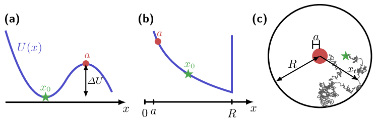
Figure 1: Crossing of a free energy barrier. (a) Energy landscape $U(x)$ from a local potential minimum $a$ over a barrier $a$ with barrier height $\varDelta U$. (b) Geometry-induced potential $U(x)=-(d-1)\ln x$ for a diffusive search in a $d$-dimensional domain with radius $R$ as illustrated in (c).

The chapter is organized as follows. Generic single-molecule FPT concepts are introduced in Sec. 1. Section 2 outlines a spectral expansion of the FPT density. Section 3 relates the single-molecule FPT problem to the corresponding many-particle problem, while two examples of FPT statistics in discrete- and continuous state-space dynamics are presented in Sec. 4. In working out these examples we utilize a recently proven duality between first passage and relaxation processes – an algorithmic tool that allows determining the full first passage time distribution analytically from a simpler relaxation process (Appendix 0.A). We conclude with an outlook in Sec. 3.

2 First passage time statistics

1 The single-particle setting

Let $x_{t}$ denote the dynamics of a reaction coordinate, e.g., the position of a particle in a potential $U(x)$ (see Fig. 1a) or in a circular domain with a central target (see Fig. 1b,c). Suppose that $x_{t}$ obeys a Markovian equation of motion. The reaction kinetics are then characterized by the FPT – the first instance $x_{t}$ reaches a given threshold $a$, defined formally as

$$t_{a}(x_{0})=\min\{t|x_{t}=a\}.$$ (1)

The stochasticity of $x_{t}$ renders the FPT, $t_{a}(x_{0})$, a stochastic variable. The statistics of $t_{a}(x_{0})$ is fully characterized by the survival probability

$$\mathcal{P}_{a}(t|x_{0})\equiv\operatorname{Prob}[t_{a}(x_{0})\geq t],$$ (2)

which quantifies the probability that the reaction did not occur before $t$. $\mathcal{P}_{a}(t|x_{0})$ decays monotonically from $\mathcal{P}_{a}(t|x_{0})=1$ to $\mathcal{P}_{a}(t{=}\infty|x_{0})=0$ with a slope that is nothing but the first passage time density

$$\wp_{a}(t|x_{0})\equiv-\frac{\partial}{\partial t}\mathcal{P}_{a}(t|x_{0}).$$ (3)

The $k$th moment of $t_{a}(x_{0})$ can be determined via

$$\langle t_{a}(x_{0})^{k}\rangle=\int_{0}^{\infty}t^{k}\wp_{a}(t|x_{0})\mathrm{d}t=k\int_{0}^{\infty}t^{k-1}\mathcal{P}_{a}(t|x_{0})\mathrm{d}t,$$ (4)

where the last equality follows from Eq. (3) by partial integration. Notably, $\langle t_{a}(x_{0})^{k}\rangle$ are typically dominated by the long-time behavior of $\wp_{a}(t|x_{0})$ [33, 30]. While the full FPT density is generally hard to determine, simple integral formulas exist for the moments of the FPT under diffusive dynamics [36].

However, as we show later, the moments of the FPT in the single-particle setting in fact provide very little information about the kinetics in many-particle systems. Namely, few-encounter and nucleation kinetics for example, are typically governed by short [34, 35] or intermediate time-scales [33].

2 Spectral expansion of first passage distributions

For reversible Markovian dynamics the FPT density allows the expansion

$$\wp_{a}(t|x_{0})=\sum_{k>0}w_{k}(x_{0})\mu_{k}\mathrm{e}^{-\mu_{k}t},$$ (5)

where $\mu_{k}^{-1}$ denotes the $k$th first passage time-scale such that $\mu_{k}$ is a rate, and $w_{k}(x_{0})$ is the corresponding weight of the $k$th mode. In contrast to $\mu_{k}$, $w_{k}(x_{0})$ depends on the starting position $x_{0}$. For convenience, we drop the functional dependence of both $w_{k}$ and $\mu_{k}$ on $a$. The weights satisfy the normalization condition $\sum_{k}w_{k}(x_{0})=1$, and the positivity of $\wp_{a}(t|x_{0})$ implies $w_{1}>0$. Specifically, if energetic or kinetic barriers are high enough a separation of time-scales emerges ($\mu_{2}\gg\mu_{1}$), such that the FPT distribution becomes approximately $\wp_{a}(t|x_{0})\simeq w_{1}(x_{0})\mu_{1}\mathrm{e}^{-\mu_{1}t}$ with $w_{1}(x_{0})\simeq 1$ if $x_{0}$ is located before the highest energy barrier [30]. Note that for finite discrete-state systems the sum in Eq. (5) is finite. The survival probability analogously becomes

$$\mathcal{P}_{a}(t|x_{0})=\int_{t}^{\infty}\wp_{a}(t^{\prime}|x_{0})\mathrm{d}t^{\prime}=\sum_{k>0}w_{k}(x_{0})\mathrm{e}^{-\mu_{k}t}.$$ (6)

Using the spectral expansion the Laplace transform of $\wp_{a}(t|x_{0})$ reads

$$\tilde{\wp}_{a}(s|x_{0})=\int_{0}^{\infty}\mathrm{e}^{-st}\wp_{a}(t|x_{0})\mathrm{d}t=\sum_{k>0}\frac{w_{k}(x_{0})\mu_{k}}{s+\mu_{k}}.$$ (7)

and the $k$th moment of the single-particle first passage time is given by

$$\langle t_{a}(x_{0})^{k}\rangle=k!\sum_{i>0}w_{i}(x_{0})\mu_{i}^{-k}.$$ (8)

When $\mu_{2}\gg\mu_{1}$, $\langle t_{a}(x_{0})^{k}\rangle$ is typically dominated by the slowest time scale, i.e., $\langle t_{a}(x_{0})^{k}\rangle\simeq k!w_{1}(x_{0})/\mu_{1}^{k}$, which is usually quite accurate in problems such as the one used in Fig. 1 (see also Ref. 33).

In general it can be difficult to determine both, first passage eigenvalues $\{\mu_{k}(x)\}$ and their corresponding weights $\{w_{k}(x)\}$. However, we have recently derived an analytical theory that allows us to determine the spectral representation of $\wp_{a}(t|x_{0})$ from the corresponding dual relaxation spectrum [33, 37], which is summarized in Appendix 0.A.

3 The many-particle setting and kinetics in the few-encounter limit

Suppose that now $n$ particles starting from the same position $x_{0}$ at time $t=0$ are searching independently for the same target. Once the first molecule hits the target a “catastrophic” response is triggered (e.g., aggregation of misfolded of proteins, induction/inhibition of gene transcription etc.), or the target disappears such as in foraging problems. In order to understand such “nucleation-type phenomena” details about the first passage time distribution become relevant [28, 12, 30, 38]. The $n$-particle survival probability is simply the product of the single particle survival probabilities [21]

$$\mathcal{P}_{a}^{(n)}(t|x_{0})\equiv\mathcal{P}_{a}(t|x_{0})^{n}.$$ (9)

The probability density that the first of the $n$ particles hits $a$ for the first time at time $t$ then becomes using Eqs. (3) and (9) [21, 33, 37]

$$\!\!\wp_{a}^{(n)}(t|x_{0})\equiv n\wp_{a}(t|x_{0})\mathcal{P}_{a}(t|x_{0})^{n-1}=n\wp_{a}^{(n)}(t|x_{0})\left[\int_{t}^{\infty}\!\!\wp_{a}(\tau|x_{0})\mathrm{d}\tau\right]^{n-1}.$$ (10)

We will henceforth omit the superscript $(1)$ in denoting the single-particle scenario, i.e., $\wp_{a}\equiv\wp_{a}^{(1)}$ and $\langle\cdots\rangle\equiv\langle\cdots\rangle^{(1)}$.

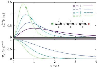
Figure 2: $n$-particle density $\wp_{a}^{(n)}(t|x_{0})$ (top) and the second term in the product of Eq. (10), $\mathcal{P}_{a}(t|x_{0})^{n-1}$, (bottom) for a four-state random walk. Diamonds depict the respective mean FPTs. More details about $\wp_{a}$ and $\mathcal{P}_{a}$ are given in Sec. 5.

Analogously to Eq. (4), the moments of the first passage time in the $n$-particle case read

$$\langle t_{a}(x_{0})^{k}\rangle^{(n)}\equiv\int_{0}^{\infty}t^{k}\wp_{a}^{(n)}(t|x_{0})\mathrm{d}t,$$ (11)

which according to Eq. (10) can be determined solely from $\wp_{a}(t|x_{0})$

$$\langle t_{a}(x_{0})^{k}\rangle^{(n)} =n\langle t_{a}(x_{0})^{k}\mathcal{P}_{a}[t_{a}(x_{0})|x_{0}]^{n-1}\rangle$$

$$=n\int_{0}^{\infty}t^{k}\mathcal{P}_{a}(t|x_{0})^{n-1}\wp_{a}(t|x_{0})\mathrm{d}t.$$ (12)

Due to the term $\mathcal{P}_{a}(t|x_{0})^{n-1}$ in Eq. (12) one needs, for any finite value of $k\geq 1$, formally an infinite number of single-particle moments, to determine $\langle t_{a}(x_{0})^{k}\rangle^{(n)}$. Hence, many-particle nucleation-type kinetics cannot be understood in terms of single-particle mean first passage times [34, 35, 33].

Even if $\langle t_{a}(x_{0})^{k}\rangle$ is accurately characterized by long-time asymptotics, the latter do not provide accurate results for $\langle t_{a}(x_{0})^{k}\rangle^{(n)}$, which can be orders of magnitude off [33]. The severe insufficiency of single-particle moments arises from the sharp sigmoidal shape of $\mathcal{P}_{a}(t|x_{0})^{n-1}$ within the many-particle average (12) (e.g., see lower panel of Fig. 2 for an illustration). We note that utilizing long-time asymptotics can lead in general to both an overestimation or an underestimation of $\langle t_{a}(x_{0})^{k}\rangle^{(n)}$, depending on the initial conditions [33]. For $n\to\infty$ short-time asymptotics sets in, for which it has been found that $\langle t_{a}(x_{0})\rangle^{(n)}\propto 1/\ln(n)$ for overdamped diffusive first passage problems [34, 35] (see also Ref. 21).

Two generic phenomena emerge as the particle number $n$ increases: (i) $\langle t_{a}(x_{0})\rangle^{(n)}$ reduces and (ii) the width of $\wp_{a}^{(n)}(t|x_{0})$ concurrently decreases (see Fig. 2). Both are independent of the details of dynamics and directly follow from a progressively sigmoidal shape of $\mathcal{P}_{a}(t|x_{0})^{n-1}$. These features are particularly important for explaining the so-called proximity effect – the spatial proximity of co-regulated genes – in transcription regulation [30]. The generic origin of these effects provides an explanation of the robustness of the proximity effect (see Ref. 30 for more details on the biological aspect).

4 Determining first passage time statistics from relaxation spectra

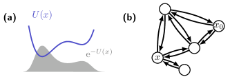
Figure 3: Schematic of (a) diffusive dynamics and (b) Markovian jump-process.

Having established that the full FPT statistics are required for a correct physical description of reaction kinetics in the few-encounter limit, we now present, on the hand of two illustrative examples, a canonical method to determine $\wp_{a}(t|x_{0})$ from the corresponding relaxation spectrum.

We consider two classes of processes, diffusion in effectively one-dimensional potentials and reversible Markovian jump-processes, in more detail (see e.g. Fig. 3). We call $x_{t}$ a relaxation process if, in contrast to the first passage problem, the dynamics does not terminate upon reaching a threshold. More precisely, for a diffusion process (see Fig. 3a) the probability density $P(x,t|x_{0})$ to find a particle starting from $x_{0}$ at position $x$ at time $t$ satisfies the Fokker-Planck equation

$$\frac{\partial}{\partial t}P(x,t|x_{0})=\hat{L}_{\text{FP}}P(x,t|x_{0})\equiv\frac{\partial}{\partial x}D(x)\Big{[}U^{\prime}(x)+\frac{\partial}{\partial x}\Big{]}P(x,t|x_{0}),$$ (13)

where $U(x)$ is the potential $(U^{\prime}\equiv\partial_{x}U)$ and $D(x)$ the diffusion landscape. Relaxation dynamics conserves probability, i.e., $\int P(x,t|x_{0})\mathrm{d}x=1$ for all $t$, which is obtained either with natural boundary condition or a “reflecting barrier”, which would in turn imply $[U(x)-\partial_{x}]P(x,t|x_{0})|_{x=a}=0$. For jump-processes (see Fig. 3b) the probability to find the system at state $x_{t}=x$ if it started at $x_{0}$ obeys a master equation

$$\frac{\partial}{\partial t}P(x,t|x_{0})=\hat{L}_{\text{ME}}P(x,t|x_{0})\equiv\sum_{x^{\prime}}L_{xx^{\prime}}P(x^{\prime},t|x_{0}),$$ (14)

where $L_{xx^{\prime}}$ is the transition rate from state $x^{\prime}$ to $x$ if $x\neq x^{\prime}$ and $L_{xx}=-\sum_{x^{\prime}\neq x}L_{x^{\prime}x}$ is the negative rate of leaving state $x^{\prime}$, guaranteeing conservation of probability $\sum_{x}L_{xx^{\prime}}=0$, i.e., $\sum_{x}P(x,t|x^{\prime})=1$ for all $t$ and $x^{\prime}$. Moreover, reversibility requires the rates to obey detailed balance $\ln(L_{xx^{\prime}}/L_{x^{\prime}x})=U(x^{\prime})-U(x)$ [39]. Both classes of reversible stochastic dynamics allow an expansion of the operator $\hat{L}=\hat{L}_{\text{FP}},\hat{L}_{\text{ME}}$ in a real bi-orthogonal eigenbasis, such that

$$P(x,t|x_{0})=\sum_{k\geq 0}\psi_{k}^{\mathrm{R}}(x)\psi_{k}^{\mathrm{L}}(x_{0})\mathrm{e}^{-\lambda_{k}t},$$ (15)

where $\lambda_{k}$ is the $k$th eigenvalue of operator $\hat{L}$ (with $0=\lambda_{0}<\lambda_{1}\leq\lambda_{2}\leq\ldots$), and $\psi_{k}^{\mathrm{R}}$ ($\psi_{k}^{\mathrm{L}}$) are the corresponding right (left) eigenvectors satisfying $\hat{L}\psi_{k}^{\mathrm{R}}=-\lambda_{k}\psi_{k}^{\mathrm{R}}$ and $\psi_{k}^{\mathrm{L}}(x)=\mathcal{N}_{k}^{-1}\mathrm{e}^{U(x)}\psi_{k}^{\mathrm{R}}(x)$. The normalization for $\hat{L}=\hat{L}_{\mathrm{FP}}$ reads $\mathcal{N}_{k}=\int\mathrm{e}^{U(x)}[\psi_{k}^{\mathrm{R}}(x)]^{2}\mathrm{d}x$, whereas for $\hat{L}=\hat{L}_{\mathrm{ME}}$ the integral in $x$ becomes a sum. Note that the zeroth eigenvector ($k=0$) is given by $\psi_{0}^{\mathrm{R}}(x)=\mathrm{e}^{-U(x)}$, such that $\psi_{0}^{\mathrm{R}}(x)\psi_{0}^{\mathrm{L}}(x_{0})=P^{\text{eq}}(x)$ is the Boltzmann distribution.

The terms $k>0$ in the sum of Eq. (15) relax to zero exponentially fast with rates $\lambda_{k}$, and the corresponding eigenfunctions $\psi_{k}^{\mathrm{R}}(x)\psi_{k}^{\mathrm{L}}(x_{0})$ quantify the redistribution of the probability mass. For potential landscapes with $n$ energy basins (e.g., $n=2$ in left panel of Fig. 3) we generally expect at least one (or the last) gap at $\lambda_{n-1}\ll\lambda_{n}$ in the relaxation spectrum.

For any stationary Markov process the renewal theorem [40]

$$P(a,t|x_{0})=\int_{0}^{t}P(a,t-\tau|a)\wp_{a}(\tau|x_{0})\mathrm{d}\tau,$$ (16)

connects the propagator of relaxation dynamics to the FPT density. It has the following intuitive interpretation: if a particle starting from $x_{0}$ is found at position $x_{t}=a$ at time $t$, then it must have reached it for the first time before that time $\tau\leq t$ and then returned to (or stayed at) $a$ in the remaining time interval $t-\tau$. Laplace transforming Eq. (16), where a convolution in the time domain becomes a product, translates Eq. (16) to $\tilde{P}(a,s|x_{0})=\tilde{P}(a,s|a)\tilde{\wp}_{a}(s|x_{0})$, i.e.,

$$\tilde{\wp}_{a}(s|x_{0})=\frac{\tilde{P}(a,s|x_{0})}{\tilde{P}(a,s|a)}.$$ (17)

Comparing Eq. (17) with the first passage density (7) one can easily verify that poles of the first passage time distribution $\tilde{\wp}_{a}(s|x_{0})$, which are located at the first passage rates $\mu_{k}=-s$, are zeros of the diagonal of the propagator $\tilde{P}(a,s|a)$ [41].

In Appendix 0.A we present an explicit and exact duality relation that allows for an explicit inversion of Eq. (17) to the time domain. Briefly, $\wp_{a}(t|x_{0})$ is obtained in three steps: (i) the first step is to realize that the first passage and relaxation time-scales interlace, $\lambda_{k-1}\leq\mu_{k}\leq\lambda_{k}$, which is then utilized in (ii) the second step to express all first passage rates $\{\mu_{k}\}$ in terms of series of determinants of almost triangular matrices (23). (iii) The third an final step involves the Chauchy residue theorem to determine the first passage weights $\{w_{k}\}$ from Eq. (28), leading to

$$w_{k}(x_{0})=\frac{\sum_{l\geq 0}(1-\lambda_{l}/\mu_{k})^{-1}\psi^{\mathrm{R}}_{l}(a)\psi^{\mathrm{L}}_{l}(x_{0})}{\sum_{l\geq 0}(1-\lambda_{l}/\mu_{k})^{-2}\psi^{\mathrm{R}}_{l}(a)\psi^{\mathrm{L}}_{l}(a)}.$$ (18)

For the full details we refer the reader to Appendix 0.A or Refs. 33, 37. In the following we apply the duality to determine FPT densities of a simple four-state Markov process and a diffusion in a rugged potential.

5 Four state Markov jump process

For illustratory purposes we consider a simple four state biased random walk as shown in the inset of Fig. 2 with a transition matrix

$$\mathbf{L}=\begin{pmatrix}-2&1&0&0\\ 2&-3&1&0\\ 0&2&-3&1\\ 0&0&2&-1\\ \end{pmatrix},$$ (19)

whose eigenvalues are $\{\lambda_{0},\lambda_{1},\lambda_{2},\lambda_{3}\}=\{0,1,3,5\}$ and the corresponding eigenvectors can be obtained in a straightforward manner. We fix the initial and target state to $x_{0}=1$ and $a=4$, respectively. The diagonal and off-diagonal relaxation propagators then have the simple forms

$$P(a,t|a) =\frac{8}{15}+\frac{\mathrm{e}^{-t}}{4}+\frac{\mathrm{e}^{-3t}}{6}+\frac{\mathrm{e}^{-5t}}{20}$$ (20)

$$P(a,t|x_{0}) =\frac{8}{15}+\mathrm{e}^{-t}+\frac{2\mathrm{e}^{-3t}}{3}+\frac{\mathrm{e}^{-5t}}{5},$$

whereas a similarly compact analytical formula for $\wp_{a}(t|x_{0})$ cannot be found. In Appendix 2 we use the duality between relaxation and first passage processes to determine $\{\mu_{1},\mu_{2},\mu_{3}\}\simeq\{0.657,2.529,4.814\}$ and $\{w_{1}(x_{0}),w_{2}(x_{0}),w_{3}(x_{0})\}\simeq\{1.565,-0.740,0.175\}$. The resulting single-particle FPT probability density is depicted with the solid line in the upper panel of Fig. 2. The dash-dotted line (here $n=2$) in the lower panel depicts the corresponding single-particle survival probability $\mathcal{P}_{a}(t|x_{0})$. We note that the short-time limit yields $\wp_{a}(t|x_{0})=4t^{2}+\mathcal{O}(t)^{3}$, which is arises from the two intermediate states between $x_{0}$ and $a$ (see model scheme from Fig. 2). The vanishing first passage density $\wp_{a}\to 0$ (short-time limit) causes a strong narrowing of the many-particle first passage density $\wp_{a}^{(n)}(t|x_{0})=n\wp_{a}(t|x_{0})\mathcal{P}_{a}(t|x_{0})^{n-1}$, since the survival probability “pushes” the probability mass to short times for increasing values of $n$ (see Fig. 2).

6 Diffusive exploration of a rugged energy landscape

As a second example we analyze $\wp_{a}(t|x_{0})$ for a diffusive barrier crossing in a rugged multi-well potential, which is particularly relevant for protein folding and misfolding kinetics [42, 43, 44, 45] and biochemical association reactions [46].

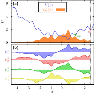
Figure 4: (a) Rugged potential landscape $U(x)$ from Eq. (21) and the corresponding Boltzmann measure with $(z_{1},\ldots,z_{7})=(-0.14,-1.04,0.77,-1.32,-0.61,-1.66,-2.67)$. (b) The first four excited right eigenfunctions corresponding to $U(x)$ with $D(x)=1$.

We generate a single rugged potential landscape as a sum of a harmonic potential and a truncated Karhunen-Loève expansion of a Wiener process

$$U(x)=\frac{x^{2}}{4}+\sum_{k=1}^{N}z_{k}\frac{\sin[(2k-1)x]}{(2k-1)}.$$ (21)

We truncate the expansion at $N=7$ and sample $z_{k}$ from a normal distribution. Once $\{z_{k}\}$ are determined, they are kept fixed. In Fig. 4a we depict $U(x)$ and its corresponding equilibrium probability density $\psi_{0}^{\mathrm{R}}(x)\propto\mathrm{e}^{-U(x)}$. We numerically determine the first 45 eigenvalues $\{\lambda_{k}\}$ and eigenfunctions $\{\psi_{k}^{\mathrm{R}}\}$ of the Fokker-Planck operator (13), from which the first four excited relaxation eigenmodes are illustrated in Fig. 4b. The relaxation eigenfunctions determine the redistribution of probability during the approach to equilibrium. Using the Newton’s series of almost triangular matrices from Eq. (23) we determine the first passage time-scales $\mu_{k}^{-1}$, which interlace with the relaxation time-scales [33, 37] as illustrated in the upper panel of Fig. 5. Specifically, between any two consecutive first passage time scales (blue circles) we find exactly one relaxation time-scale (red triangles) and vice versa. In particular, the slowest first passage time-scale occurs on a longer time-scale than the slowest relaxation time-scale. This can be explained by the fact that the slowest first passage mode requires all trajectories to reach the target, whereas the slowest relaxation mode only reflects that most trajectories have reached the equilibrium distribution.

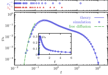
Figure 5: The FPT density for particle starting from $x_{0}=0.6$ and to $a=2.5$ within potential from Fig. 4. The inset shows the first passage time density on a linear scale. The upper panel superimposes the first passage time scales $\mu_{k}^{-1}$ (open circles) and the relaxation time scales $\lambda_{k}^{-1}$ (open triangles). The symbols are obtained using the theory outlined in Appendix 0.A, and the symbols denote results of Brownian dynamics simulations of $10^{6}$ trajectories.

In the lower panel of Fig. 5 we present results for the full FPT density using the analytical theory from Appendix 0.A (blue solid line), together with results of extensive Brownian dynamics simulations of $10^{6}$ trajectories, which perfectly agree with the theory. The inset depicts $\wp_{a}(t|x_{0})$ on linear scale. The short-time limit for a freely diffusing particle in form of a Lévi-Smirnov density, also know as Sparre Anderson result [47, 30], is shown as dashed green line (see also Refs. 34, 35, 21 for further discussions on the short-time limit). Intuitively, diffusion is faster than advection on short time-scales ($\propto\sqrt{t}$ vs. $\propto t$ behavior), rendering the actual potential shape less relevant for $t\to 0$.

3 Concluding perspectives

The mean and higher moments of the FPT in a single-particle setting were shown to be inherently insufficient for characterizing many-particle FPT kinetics within the few-encounter limit. To correctly describe few-encounter kinetics one has to go beyond a description limited to FPT moments and determine the full FPT distribution. It was shown how to achieve this utilizing a duality relation between relaxation and first passage process [33, 37] outlined in Appendix 0.A. The method is applicable to a broad class of reversible Markov dynamics that includes discrete Markovian jump-processes in any dimension and Markovian diffusion in effectively one-dimensional potential landscapes.

The duality relation can in fact be considered as an analytical algorithmic tool for determining FPT distributions, which was demonstrated on hand of a simple four state model in full detail. The analysis of the $n$-particle FPT distribution revealed a reduced mean FPT and a canonical narrowing of the FPT distribution in the few-encounter limit as the number of particle increases. This narrowing arises due to a combination of the short-time cutoff in the FPT density ($\wp_{a}\to 0$ for $t\to 0$) and an inherent many-particle speed-up, which together render the $n$-particle kinetics deterministic in the limit $n\to\infty$. In the case of a diffusive exploration of (rugged) energy landscapes the short-time behavior is dominated by free diffusion, rendering the shape of the potential essentially irrelevant[34, 35].

It will be interesting to extend the applications of the theory outlined in Appendix 0.A and to explore the physical consequences of few-encounter kinetics also in narrow escape problems [48, 49, 50, 51, 52, 53] and diffusion on higher-dimensional graphs. Extending the work to irreversible dynamics will be challenging, whereas long-time asymptotics are still accessible [30, 37].

Appendix 0.A Duality between relaxation and first passage processes

1 General case

In this appendix we review the duality relation from Refs. 33, 37 that allows us to determine analytically the spectral representation of the FPT density in Eq. (5) from the propagator in Eq. (15) in three steps.

The first step is to realize that the relaxation time-scales $\{\lambda_{k}^{-1}\}$ and first passage times-scales $\mu_{k}^{-1}$ interlace [33, 37]

$$\lambda_{k-1}\leq\mu_{k}\leq\lambda_{k}.$$ (22)

We note that this interlacing of time-scales can be related to Chauchy’s interlacing theorem for real symmetric matrices [54]. The interlacing has also been demonstrated for simple one-dimensional processes [41].

The second step is based on an explicit Newton iteration that allows, after to some rather involved algebra [33, 37], to exactly express the first passage rates $\mu_{k}$ as a series of determinants of almost triangular matrices $\boldsymbol{\mathcal{A}}_{n}(k)$

$$\mu_{k}=\bar{\mu}_{k}+\sum_{n=1}^{\infty}f_{0}(k)^{n}f_{1}(k)^{1-2n}\det\boldsymbol{\mathcal{A}}_{n}(k),$$ (23)

where $\bar{\mu}_{k}\equiv(\lambda_{k}+\lambda_{k-1})/2$, $f_{n}(k)=\partial_{s}^{n}F(k^{*},s)|_{s=-\bar{\mu}_{k}}$ with

$$F(k,s)=(s+\lambda_{k})\tilde{P}(a,s|a)$$ (24)

and the index function

$$k^{*}\equiv k^{*}(k)=\begin{cases}k&\text{if $F(k,-\bar{\mu}_{k})<0$},\\ k-1&\text{else}\end{cases}$$ (25)

that guarantees $f_{0}(k)$ to be negative, and we used the almost triangular $(n-1)\times(n-1)$ matrices with elements

$$\mathcal{A}_{n}^{i,j}(k)=\frac{f_{i-j+2}(k)\Theta(i-j+1)}{(i-j+2)!}\begin{cases}i+j-1&\text{if $j=1$,}\\ n(i-j+1)+j-1&\text{if $j>1$,}\end{cases}$$ (26)

where $\Theta$ is the discrete Heaviside step function ($\Theta(l)=1$ if $l\geq 0$) and $\det\boldsymbol{\mathcal{A}}_{1}(k)=1$. Moreover, we have explicitly [33, 37]

$$f_{0}(k) =\psi^{\mathrm{L}}_{k^{*}}(a)\psi_{k^{*}}^{\mathrm{R}}(a)+\sum_{l|l\neq k^{*}}\psi^{\mathrm{L}}_{l}(a)\psi_{l}^{\mathrm{R}}(a)\frac{(\bar{\mu}_{k}-\lambda_{k^{*}})}{(\bar{\mu}_{k}-\lambda_{l})},$$ (27)

$$f_{n\geq 1}(k) =n!\sum_{l|l\neq k^{*}}\psi^{\mathrm{L}}_{l}(a)\psi_{l}^{\mathrm{R}}(a)\frac{(\lambda_{l}-\lambda_{k^{*}})}{(\bar{\mu}_{k}-\lambda_{l})^{n+1}}.$$

The third step is a straightforward application of the residue theorem, delivering the first passage weights

$$w_{k}(x_{0})=\frac{\tilde{P}(a,s|x_{0})}{\mu_{k}\partial_{s}\tilde{P}(a,s|a)}\bigg{|}_{s=-\mu_{k}}=\frac{\sum_{l\geq 0}(1-\lambda_{l}/\mu_{k})^{-1}\psi^{\mathrm{R}}_{l}(a)\psi^{\mathrm{L}}_{l}(x_{0})}{\sum_{l\geq 0}(1-\lambda_{l}/\mu_{k})^{-2}\psi^{\mathrm{R}}_{l}(a)\psi^{\mathrm{L}}_{l}(a)},$$ (28)

where $\tilde{P}(a,s|x_{0})$ is the Laplace transform of Eq. (20). We note that Eq. (23) and (28) are exact relations that fully characterize the first passage kinetics.

2 Four state model

We now evaluate $\wp_{a}(t|x_{0})$ for the model from Sec. 5 step by step. First, the Laplace transform of the first line of Eq. (20), $\tilde{P}(a,s|a)$, is inserted into Eqs. (24) and (25) giving $k^{*}=k$ for $k=1,2,3$. Second, Eq. (27) yields

$$\begin{pmatrix}f_{0}(1)\\ f_{0}(2)\\ f_{0}(3)\end{pmatrix}=\begin{pmatrix}-\frac{11}{45}\\ -\frac{1}{3}\\ -\frac{1}{3}\end{pmatrix},\qquad\begin{pmatrix}\frac{f_{n}(1)}{n!}\\ \frac{f_{n}(2)}{n!}\\ \frac{f_{n}(3)}{n!}\end{pmatrix}=\begin{pmatrix}\frac{1}{3}(-\frac{2}{5})^{n+1}+\frac{1}{5}(-\frac{2}{9})^{n+1}-\frac{2^{n+4}}{15}\\ \frac{1}{10}[(-3)^{-n-1}-2^{3-n}-5]\\ \frac{1}{3}[-2^{1-2n}-3^{-n}-1]\end{pmatrix}$$ (29)

with $n>0$. Note that $k^{*}$ is chosen to guarantee the negativity of $f_{0}(k)$. Third, inserting the $f_{n}(k)/n!$ into the almost triangular matrix Eq. (26) and evaluating the Newton’s series (23) yields the exact first passage time-scales, which numerically are given by $\{\mu_{1},\mu_{2},\mu_{3}\}\simeq\{0.657,2.529,4.814\}$. Finally, the weights from Eq. (28) yield $\{w_{1}(x_{0}),w_{2}(x_{0}),w_{3}(x_{0})\}\simeq\{1.565,-0.740,0.175\}$, which fully determines $\wp_{a}(t|x_{0})$.

Acknowledgements

The financial support from the German Research Foundation (DFG) through the Emmy Noether Program “GO 2762/1-1” (to AG) is gratefully acknowledged.

References

- 1. M. von Smoluchowski, Phys. Z., 17, 557–585 (1916).
- 2. H. Kramers, Physica, 7, 284–304 (1940).
- 3. A. Szabo, K. Schulten, and Z. Schulten, J. Chem. Phys., 72, 4350–4357 (1980).
- 4. E. Ben-Naim, S. Redner, and F. Leyvraz, Phys. Rev. Lett., 70, 1890–1893 (1993).
- 5. G. Oshanin, A. Stemmer, S. Luding, and A. Blumen, Phys. Rev. E, 52, 5800–5805 (1995).
- 6. T. Guérin, N. Levernier, O. Bénichou, and R. Voituriez, Nature, 534, 356–359 (2016).
- 7. Y. Li, D. Debnath, P. K. Ghosh, and F. Marchesoni, J. Chem. Phys., 146, 084104 (2017).
- 8. P. Hänggi, P. Talkner, and M. Borkovec, Rev. Mod. Phys., 62, 251–341 (1990).
- 9. S. Redner, A guide to first-passage processes. Cambridge University press, Cambridge (2001).
- 10. A. J. Bray, S. N. Majumdar, and G. Schehr, Adv. Phys., 62, 225–361 (2013).
- 11. R. Metzler, G. Oshanin, and S. Redner, eds., First-Passage Phenomena and Their Applications. World Scientific Publishing, Singapore (2014).
- 12. O. Bénichou and R. Voituriez, Phys. Rep., 539, 225–284 (2014).
- 13. R. Kopelman, Science, 241, 1620–1626 (1988).
- 14. D. ben Avraham and S. Havlin, Diffusion and Reactions in Fractals and Disordered Systems. Cambridge University Press, Cambridge (2000).
- 15. P. C. Bressloff and J. M. Newby, Rev. Mod. Phys., 85, 135–196 (2013).
- 16. A. Godec and R. Metzler, Phys. Rev. E, 91, 052134 (2015).
- 17. G. Vaccario, C. Antoine, and J. Talbot, Phys. Rev. Lett., 115, 240601 (2015).
- 18. A. Godec and R. Metzler, Sci. Rep., 6, 20349 (2016).
- 19. J.-F. Rupprecht, O. Bénichou, D. S. Grebenkov, and R. Voituriez, J. Stat. Phys., 158, 192–230 (2015).
- 20. D. S. Grebenkov, Phys. Rev. Lett., 117, 260201 (2016).
- 21. C. Mejía-Monasterio, G. Oshanin, and G. Schehr, J. Stat. Mech. (2011) P06022.
- 22. B. Munsky, I. Nemenman, and G. Bel, J. Chem. Phys., 131, 235103 (2009).
- 23. G. Bel, B. Munsky, and I. Nemenman, Phys. Biol., 7, 016003 (2010).
- 24. R. Grima and A. Leier, J. Phys. Chem. B, 121, 13–23 (2017).
- 25. D. Schnoerr, B. Cseke, R. Grima, and G. Sanguinetti, Phys. Rev. Lett., 119, 210601 (2017).
- 26. M. F. Weber and E. Frey, Rep. Prog. Phys., 80, 046601 (2017).
- 27. D. Schnoerr, G. Sanguinetti, and R. Grima, J. Phys. A: Math. Theor., 50, 093001 (2017).
- 28. O. Bénichou, C. Chevalier, J. Klafter, B. Meyer, and R. Voituriez, Nat. Chem., 2, 472–477 (2010).
- 29. B. Meyer, C. Chevalier, R. Voituriez, and O. Bénichou, Phys. Rev. E, 83, 051116 (2011).
- 30. A. Godec and R. Metzler, Phys. Rev. X, 6, 041037 (2016).
- 31. G. Kolesov, Z. Wunderlich, O. N. Laikova, M. S. Gelfand, and L. A. Mirny, Proc. Natl. Acad. Sci. USA, 104, 13948–13953 (2007).
- 32. P. Fraser and W. Bickmore, Nature, 447, 413–417 (2007).
- 33. D. Hartich and A. Godec, New J. Phys, 20, 112002 (2018).
- 34. N. G. van Kampen, J. Stat. Phys., 70, 15–23 (1993).
- 35. H. van Beijeren, J. Stat. Phys., 110, 1397–1410 (2003).
- 36. C. W. Gardiner, Handbook of Stochastic Methods, 3 edn. Springer, Berlin (2004).
- 37. D. Hartich and A. Godec, J. Stat. Mech. (2019) 024002.
- 38. D. Grebenkov, R. Metzler, and G. Oshanin, Phys. Chem. Chem. Phys., 20, 16393-16401 (2018).
- 39. N. G. van Kampen, Stochastic Processes in Physics and Chemistry, 3 edn. North-Holland Personal Library, Elsevier, Amsterdam (2007).
- 40. A. J. F. Siegert, Phys. Rev., 81, 617–623 (1951).
- 41. J. Keilson, J. Appl. Prob., 1, 247–266 (1964).
- 42. F. Noé, S. Doose, I. Daidone, M. Löllmann, M. Sauer, J. D. Chodera, and J. C. Smith, Proc. Natl. Acad. Sci. USA, 108, 4822–4827 (2011).
- 43. H. Yu, D. R. Dee, X. Liu, A. M. Brigley, I. Sosova, and M. T. Woodside, Proc. Natl. Acad. Sci. USA, 112, 8308–8313 (2015).
- 44. K. Neupane, A. P. Manuel, and M. T. Woodside, Nat. Phys., 12, 700 (2016).
- 45. D. R. Dee and M. T. Woodside, Prion, 10, 207–220 (2016).
- 46. K. Schulten, Z. Schulten, and A. Szabo, J. Chem. Phys., 74, 4426–4432 (1981).
- 47. E. Sparre Andersen, Math. Scand., 1, 263–285 (1953); Math. Scand., 2, 194–222 (1954)
- 48. A. Singer, Z. Schuss, and D. Holcman, J. Stat. Phys., 122, 465–489 (2006).
- 49. Z. Schuss, A. Singer, and D. Holcman, Proc. Natl. Acad. Sci. USA, 104, 16098–16103 (2007).
- 50. J. Reingruber and D. Holcman, Phys. Rev. Lett., 103, 148102 (2009).
- 51. S. Pillay, M. J. Ward, A. Peirce, and T. Kolokolnikov, Multiscale Model. Simul., 8, 803–835 (2010).
- 52. S. A. Isaacson, A. J. Mauro, and J. Newby, Phys. Rev. E, 94, 042414 (2016).
- 53. D. S. Grebenkov and G. Oshanin, Phys. Chem. Chem. Phys., 19, 2723–2739 (2017).
- 54. R. Grone, K. H. Hoffmann, and P. Salamon, J. Phys. A: Math. Theor., 41, 212002 (2008).