Lost in Diversification

Abstract

As financial instruments grow in complexity more and more information is neglected by risk optimization practices. This brings down a curtain of opacity on the origination of risk, that has been one of the main culprits in the 2007-2008 global financial crisis. We discuss how the loss of transparency may be quantified in bits, using information theoretic concepts. We find that i) financial transformations imply large information losses, ii) portfolios are more information sensitive than individual stocks only if fundamental analysis is sufficiently informative on the co-movement of assets, that iii) securitisation, in the relevant range of parameters, yields assets that are less information sensitive than the original stocks and that iv) when diversification (or securitisation) is at its best (i.e. when assets are uncorrelated) information losses are maximal. We also address the issue of whether pricing schemes can be introduced to deal with information losses. This is relevant for the transmission of incentives to gather information on the risk origination side. Within a simple mean variance scheme, we find that market incentives are not generally sufficient to make information harvesting sustainable.

1 Introduction

Financial innovations have been seen as a formidable tool to increase the efficiency of the market, by controlling the risk of financial assets thus easing resource allocation between investors and the real economy. Yet, several authors [1, 2, 3] have suggested that the increasing complexity of financial products may trigger the emergence of instabilities and systemic risks. The most commonly believed determinant of the 2007-2008 global financial crisis is the rise of structured financial products [4]. The formidable complexity of these type of products effectively brought down a curtain of opacity between the risk originators and the buyers of the financial products, that hid the true risks of the underlying assets (e.g. mortgages, loans, credits) [5, 6]. While the dangers of these instruments had been highlighted well before the crisis [7], most of the response to the crisis didn’t address the core issue of transparency loss implicit in financial transformations, but rather focused on ring fencing the financial system with various measures [8]. An exception to that, is the proposal [9] to build an efficient and standardized system, or a common language, through which information on the origin of risks should be easily available to all market participants. Such a financial barcode, which might be attached to any financial product, should contain all the information that is relevant in order to make realistic estimates about return and risk of the product, from the risk profiles of the building blocks to the market fundamentals. Yet, it is not clear how such barcodes should be constructed, which information they should contain and whether they should be statically or dynamically updated, when new information is available. In particular, an interesting open question is whether demand for such barcodes may ”naturally” arise and how barcodes should be priced, since without a barcode price the sellers would have no incentive for sharing the information.

Apparently, within the prevailing market efficiency hypothesis paradigm, according to which prices of any stock exchanged in the market reflects faithfully any relevant information [10, 11], these barcodes would be worthless. Indeed, for example, the price of Asset Backed Securities (ABS) were computed only on the basis of default probabilities of the underlying assets (e.g. mortgages). Even though, in principle, all the documentation about the underlying assets were available to buyers, the prices of ABS didn’t depend at all on it, with the consequence that incentives for due diligence in collecting information on the underlying by issuers were lacking [7, 6]. Yet, market information efficiency resides on the balance between traders seeking information (fundamental analysis) and traders exploiting it (technical analysis), as shown by a wealth of results in agent based modelling of financial markets (see e.g. [12]). The former profit by the fact that the information they gather grants them an excess return. Here the profits of collecting information accrue to the individual trader, while in the case of a structured financial product these are passed over to the buyer. Accordingly they should be reflected in the price. This simple logic is the basis of the present paper.

As a first step, we quantify the transparency loss by the amount of bits of information lost in diversification. Secondly, we address the issue of deriving the optimal barcode, the one that contains the maximal information on the return of the financial instrument. Then we compute the price associated to the barcode as the value of the information within a simple mean variance framework. The information loss and the barcode price are then quantified within a model system based on Gaussian variables (see [13] for an extension to binary variables). Within this framework we find that financial transformation implies large information losses and that market incentives are not generally sufficient to make information harvesting sustainable.

The remaining sections are organized as follows: in Section 2 we discuss the general setting, information and financial transformation. Then we quantify information losses for a simple model of Gaussian log-returns and address the issue of information pricing. We conclude with some general remarks.

2 The general framework

Let’s suppose we have a pool of $n$ assets, e.g. stocks, loans or mortgages, and let $\vec{X}=(X_{1},\ldots,X_{n})$ be the associated vector of (log-)returns. The values $\vec{X}$ are unknown to the inverstor, so we shall treat them as a vector of random variables, described by a probability distribution $p(\vec{X})$. We consider a situation where some side information related to the stock $X_{i}$, e.g. the income of the borrower of the loan or information on the fundamentals of asset $i$, is possibly available. This information is captured by a random variable $Y_{i}$ that, inspired by Ref. [9], we shall call the barcode associated to asset $i$. Barcodes allow investors that bought the asset, to retrieve all information that is relevant to estimate the return of the asset, in the sense that, given the barcodes $\vec{Y}$, they can use the conditional distribution $p(\vec{X}|\vec{Y})$ instead of $p(\vec{X})$. We shall use the mutual information [14]

$$I(U,V)=\mathbb{E}\left[\log\left[\frac{p(u|v)}{p(u)}\right]\right],$$ (1)

to quantify the amount of information that the knowledge of a variable $V$ provides on the random variable $U$. In Eq. (1) $p(u|v)$ is the conditional distribution of $U$ given that $V=v$ and $p(u)$ is the unconditional one. Hence, $I(X_{i},Y_{i})$ measures in bits the information that $Y_{i}$ provides on $X_{i}$ and $I(\vec{X},\vec{Y})$ measures the total amount of information that the barcodes $\vec{Y}$ provide on the returns $\vec{X}$.

2.1 Financial transformations

We consider financial transformations

$$\vec{X}\to F(X),\qquad X=\sum_{i=1}^{n}X_{i},$$ (2)

that entail pooling the $n$ assets into a single portfolio $X$ and applying a transformation $F(X)$. This generates a new financial asset with log-return $F(X)$. The simplest such transformation is the portfolio itself that delivers the average log-return

$$F_{\bar{X}}(X)\equiv\overline{X}=X/n.$$ (3)

Here, $\vec{X}$ can be the log-returns of individual stocks. In this case, $\vec{Y}$ would encode information on fundamentals (e.g. corporate structure of the firm, analysis of the sector they operate etc) for each stock.

$\overline{X}$ corresponds to the most basic diversification techniques, which entails investing a fraction $1/n$ in each of the $n$ assets, instead of investing in a single asset $X_{i}$. The benefit of diversification is that it reduces risk. For example, for $n$ i.i.d. stocks, the variance $\mathbb{V}(\overline{X})=\mathbb{V}(X_{i})/n$ is reduced by a factor of $n$, w.r.t. that of individual stocks.

Another class of products we consider are Asset Backed Securities (ABS), the typical products of structured finance [4], whose return function is based on a prioritized structure of claims. In these products, the claims over the cash flow of the returns of the underlying assets $X_{i}$ are structured in such a way that the ABS yields a positive return when the total return is larger then a given threshold $k$. The return of these products is

$$F_{k}(X)=\theta\left(X-k\right),$$ (4)

where $\theta(x)=1$ when $x\geq 0$ and $\theta(x)=0$ otherwise. Different tranches correspond to different risk profiles that can be obtained with different values of $k$. The transformation $\vec{X}\to F_{k}(X)$ is an example of securitisation and the advantage of it is that it turns a set of risky assets $X_{i}$ into assets with a controlled risk profile. Sufficiently small values of $k$ yield assets that are very safe, i.e. for which $F_{k}(X)=1$ with high probability. As an example, mortgage backed securities (MBS) [4] are based on a portfolio $\vec{X}$ of mortgages granted to $n$ households, where $X_{i}=+1$ if household $i$ repays the mortgage and $X_{i}=0$ if $i$ defaults. In this case $Y_{i}$ may encode the occupational status of $i$, the characteristics of the neighbourhood of the house bought with the $i^{\rm th}$ mortgage. In this case, $i$’s default may occur for idiosyncratic reasons, or for systemic ones (e.g. crisis in the sector of the economy of the company where Mr. $i$ works or a natural disaster in that region) that may affect different households in the same way.

Investors can transmit all the information $\vec{Y}$ about the individual assets to the buyers of the engineered asset $F$. Yet, some of this information may not be relevant to estimate the return $F(X)$, i.e. all the information relevant to estimate the return of $F$ may be compressed in a single variable $G_{F}$ that we call the barcode of $F$. Clearly, $G_{F}(\vec{Y})$ has to be a function of $\vec{Y}$, and, ideally, the barcode $G_{F}$ should be the simplest among all possible variables $V(\vec{Y})$ such that $I\left(F(X),V(\vec{Y})\right)=I\left(F(X),\vec{Y}\right)$.

A general result can be obtained by invoking the data processing inequality [14]. This states that in any transformation $\vec{X}\to F(X)$ some information may or may not be lost, but for sure no information can be gained. In terms of the mutual information this reads

$$I(F(X),G_{F}(\vec{Y}))\leq I(F(X),\vec{Y})\leq I(X,\vec{Y})\leq I(\vec{X},\vec{Y}).$$ (5)

The term on the right end of this chain of inequalities quantifies the total amount of information in bits that barcodes $\vec{Y}$ provide on the log-returns $\vec{X}$. In the typical case of weakly dependent assets, this is proportional to the number $n$ of assets. By contrast, the second term from the right is upper bounded by the entropy of the random variable $X$, which grows at most as $\log n$. Hence, generally, financial transformations imply information losses. The choice of the optimal barcode $G_{F}(\vec{Y})$ can only mitigate further information losses, and at most saturate the leftmost inequality in Eq. (5).

In the next section we shall turn to the quantitative analysis of a representative case.

3 Barcoding finance in a Gaussian world

Let’s assume that

$$X_{i} = \mu+\xi_{i}+a\xi_{0}+JY_{i}$$ (6)

$$Y_{i} = \eta_{i}+c\eta_{0}$$ (7)

where $\mu>0$ is a positive constant, and $\xi_{i}$’s and $\eta_{i}$’s are i.i.d. Gaussian random variables with mean zero and variance one for $i=0,1,\ldots,n$. This corresponds to a one-factor model, where the covariance $\mathbb{E}[(X_{i}-\mu)(X_{j}-\mu)]=a^{2}+J^{2}c^{2}$ between assets can partly be explained by the barcode variables ($c\neq 0$). Notice also that all assets are equivalent, i.e. the distribution of $(\vec{X},\vec{Y})$ is invariant under permutations of the assets.

The mutual information on individual assets is given by

$$I(X_{i},Y_{i})=\frac{1}{2}\log\left(1+J^{2}\frac{1+c^{2}}{1+a^{2}}\right)$$ (8)

whereas the total information that barcodes provide on $\vec{X}$ is

$$I(\vec{X},\vec{Y})=\frac{n-1}{2}\log(1+J^{2})+\frac{1}{2}\log\left(1+J^{2}\frac{1+nc^{2}}{1+na^{2}}\right).$$ (9)

Since

$$X=n\mu+\sum_{i=1}^{n}\xi_{i}+na\xi_{0}+JY,\qquad Y=\sum_{i=1}^{n}Y_{i},$$ (10)

then the optimal barcode for any $F(X)$ is $G_{F}(\vec{Y})=Y$. Indeed, $I(F(X),\vec{Y})=I(F(X),Y)$, which saturates the leftmost inequality in Eq. (5). The upper bound on the information content of the barcode is given by

$$I(X,Y)=\frac{1}{2}\log\left(1+J^{2}\frac{1+nc^{2}}{1+na^{2}}\right).$$ (11)

We notice that:

1. The barcode’s information on the portfolio log-return $X$ is larger than that on individual assets (i.e. $I(X,Y)>I(X_{i},Y_{i})$) only if $c>a$, i.e. if barcodes are sufficiently informative on the co-movement of assets.

2. $I(X,Y)$ equals the second term in Eq. (9). Therefore the total loss of information is upper bounded by the first term on the right hand side of Eq. (9), which increases linearly with $n$.

3. The total loss of information $I(\vec{X},\vec{Y})-I(X,Y)$ is independent of $a$ and $c$, because all the available information on the co-movement of stocks is captured by $Y$.

4. When barcodes are not informative about the correlated variation of assets, i.e. for $c=0$, the information content of the barcode $Y$ vanishes $I(X,Y)\to 0$ as $n\to\infty$.

It is instructive to observe that, when $c\neq 0$, the barcode $Y_{j}$ provides also information on the return of asset $i$. The case when barcodes are independent ($c=0$) may be appropriate for a portfolio of stocks where $Y_{i}$ accounts only for fundamental analysis of stock $i$. In this case, very large portfolios become insensitive to information on the fundamentals of individual stocks ($I(X,Y)\to 0$ as $n\to\infty$). This is because $X$ is dominated by the common component $a\xi_{0}$ on which barcodes $Y_{i}$ provide no information. The behaviour of $I(X,Y)$ for the portfolio is summarized in the left panel of Figure 1.

The mutual information can be computed also for the ABS as follows. In a model of gaussian log-returns and information, the threshold parameter $k$ of a tranche $F_{k}$ can be related to the default probability

$$p^{k}_{d}=p(X<n\mu+k)=H\left(\frac{k}{\sqrt{\mathbb{V}(X)}}\right)$$

where $H(z)=\int_{-\infty}^{z}\frac{dz}{\sqrt{2\pi}}e^{-z^{2}/2}$ is the cumulative normal distribution function. When information $Y$ is revealed, this default probability changes into

$$p^{k}_{d}(Y)=p(X\leq n\mu+k|Y)=H\left(\frac{k-JY}{\sqrt{\mathbb{V}(X|Y)}}\right)$$

using this expression for $p^{k}_{d}(Y)$ and using Eq. (1),

$$I(F_{k},Y)=\mathbb{E}\left[p^{k}_{d}(Y)\log\frac{p^{k}_{d}(Y)}{p^{k}_{d}}+(1-p^{k}_{d}(Y))\log\frac{1-p^{k}_{d}(Y)}{1-p^{k}_{d}}\right],$$ (13)

where the expectation is taken on the distribution of $Y$. In the right panel of Figure 1 we plot the behaviour of the mutual information for the ABS. $I(F_{k},X)$ follows the same qualitative behaviour of $I(X,Y)$ although its value is considerably smaller (more than tenfold in the example of Figure 1). In addition, $I(F_{k},Y)$ decreases for safer and safer assets (i.e. as $p_{d}$ decreases), showing that most senior tranches of ABS tend to be remarkably information insensitive.

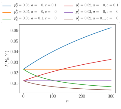
Figure 1: Mutual information $I(X,Y)$ and $I(F_{k},Y)$ of barcodes for portfolio (left) and ABS (right) generated from Gaussian underlying assets ($J=0.5$), as a function of $n$.

3.1 The cost of information: pricing barcodes

Let us now address the issue of quantifying the value of the information conveyed by the barcodes. The key question we want to address is whether the demand for barcodes can endogenously arise in a market. This is possible if barcodes can be priced in such a way that the value of the barcode of a financial instrument provides enough incentives for gathering information on the individual assets. We address this question within a mean-variance pricing scheme. Hence the setting we consider is that of a portfolio manager that gathers information on $n$ assets, and sells $n$ shares of the resulting portfolio, charging an additional amount related to the price of the information contained in the portfolio’s barcode. Investors exploit their available information about assets payoffs to price the financial product $Z=F_{Z}(X)$. When they have access to the barcode, they use the probability $p(Z|Y)$ to asses future performances of the assets, otherwise they use $p(Z)$. In a mean variance framework, the price of $X$ depends on the first two moments of $Z$. When no barcode is provided, the mean variance price reads:

$$p_{Z}=\mathbb{E}[Z]-\alpha\mathbb{V}[Z],$$ (14)

where $\alpha>0$ is the relative risk aversion coefficient. A micro-foundation of the previous formula is discussed in appendix A. As shown there, conditionally on knowing the barcode’s value $y$, the price is:

$$p_{Z|Y=y}=\mathbb{E}[Z|Y=y]-\alpha\mathbb{V}[Z|Y=y].$$ (15)

Depending on the realized information $y$, the price difference between having or not the barcode can be positive or negative. The price of the barcode should be computed before the realized value of $Y$ is known, therefore it is given by

$$\delta p_{Z}:=\mathbb{E}[p_{Z|Y}]-p_{Z}=\alpha\left\{\mathbb{V}(Z)-\mathbb{E}\left[\mathbb{V}(Z|Y)\right]\right\}=\alpha\mathbb{V}\left(\mathbb{E}[Z|Y]\right),$$ (16)

where $\mathbb{V}(Z|Y)$ is the variance of $Z$ on the distribution $p(Z|Y)$ and $\mathbb{E}[Z|Y]$ is the expected value of $Z$ conditional on the value $Y$. Eq. (16) takes the expected value over $Y$ of $\mathbb{V}(Z|Y)$ and the variance of $\mathbb{E}[Z|Y]$ over the distribution of $Y$. This result reflects the fact that the knowledge of the distribution of $Y$ does not change the unconditional expected log-return of the asset, but produces a reduction in variance which is equal to the variance of the conditional expected return.

To assess the presence of incentives for barcodes, we shall compare expected revenues from the barcode with the cost of gathering information, which is given by the cost of the barcodes of the original assets.

When log-returns are given by Eq. (6), the cost of gathering information for a single asset is

$$\delta p_{X_{i}}=\alpha J^{2}(1+c^{2}).$$ (17)

The additional log-return that the optimal barcode ${Y}=\sum_{i}{\eta_{i}}+nc\eta_{0}$ yields is

$$\delta p_{\overline{X}}=\alpha J^{2}(1/n+c^{2}).$$ (18)

Considering this as the price of the barcode that the portfolio manager can charge when selling $\overline{X}$, together with the barcode, we find that the budget’s balance for the portfolio manager for selling $n$ shares of $\overline{X}$, is

$$n\delta p_{\overline{X}}-\sum_{i=1}^{n}\delta p_{X_{i}}=-\alpha(n-1)J^{2}$$ (19)

which is negative. In words, this pricing mechanism does not provide incentives to gather information on individual assets. Interestingly, when barcodes provide information on the co-movement of the assets ($c>0$), the value of information on the whole portfolio, instead, is larger than the sum of the cost of information on individual assets, i.e.

$$\delta p_{X}-\sum_{i=1}^{n}\delta p_{X_{i}}=\alpha n(n-1)J^{2}c^{2}.$$ (20)

This is a consequence of the non-linearity of the pricing mechanism and of the fact that, for $c>0$ the barcode $Y_{i}$ of asset $i$ provides information also on other asset log-returns $X_{j}$. Indeed, there is a minimal share size, above which the barcode associated to the log-return $X/m$ provides enough incentives to gather information on individual assets in the sense that $m\delta p_{X/m}-n\delta p_{X_{i}}\geq 0$. A simple calculation shows that

$$m\leq\frac{1+J^{2}(1+nc^{2})}{1+J^{2}(1+c^{2})}.$$ (21)

The same calculation can be extended to ABS in a straightforward manner, yet the results depends on the way in which the portfolio $X$ is divided into tranches

$$X=\sum_{k}f_{k}F_{k}(X)$$ (22)

for some positive constants $f_{k}$. Then we show in appendix B that

$$\delta p_{X}>\sum_{k}\delta p_{f_{k}F_{k}(X)}.$$ (23)

This, together with the fact that for $c=0$ Eq. (20) implies that $\delta p_{X}=\sum_{i}\delta p_{X_{i}}$, shows that if barcodes do not provide information on correlated defaults, securitisation cannot provide incentives to gather information on individual assets (within the present mean variance framework). This suggests that, unless information on correlated defaults of individual assets is accounted for, securitisation decreases the value of information contained in barcodes.

4 Conclusion

In this paper we exploit information theoretic concepts to investigate the lack of transparency associated with financial transformations. We discuss a setting where side information about the returns of assets is modelled with an associated random variable, and the information content is quantified using the mutual information. In this setting, we show that every financial transformation implies information losses. In a model of Gaussian log-returns, we find that when fundamental analysis on individual assets is not informative on the co-movement of assets, the information is totally lost in the limit of very large portfolios. In addition, we show that, within a mean variance framework, the value of information also decreases, which suggests that incentives to gather information on individual assets cannot be transmitted across financial transformation. This puts serious doubts of whether market incentives alone are enough to make the introduction of a system of barcodes, as advocated in Ref. [9] sustainable.

These result generalise to a model of assets with binary returns, which is more appropriate for credit derivatives (see Ref. [13]). The aim of the present paper is that of suggesting ways forward to quantify transparency losses in finance and to raise few key issues. As such, it might be a benchmark for more complex and realistic theoretical models, or for more appropriate schemes to value information in order to overcome these issues.

Appendix A Mean variance pricing

In order to do this, we adopt a standard mean-variance framework. Consider a representative agent with an initial wealth $W$, that is facing the decision of buying $\epsilon W$ units of wealth of an asset with return $Z$. If her utility function is given by $U(\cdot)$, the certainty equivalent $w$ of this investment is defined as that value for which the investor is indifferent between investing in the asset or receiving $w$ units of wealth, i.e.

$$U(W+w)=\mathbb{E}\left[U(W+\epsilon WZ)\right],$$ (24)

where $\mathbb{E}[\ldots]$ stands for the expectation on the random variable $Z$. We take $w$ as a measure of the value of the investment that incorporates the risk premium. Assuming that $\epsilon\ll 1$ and $w\ll W$, we can expand both sides and derive, to leading order, the price of $Z$ as the value per unit of investment.

$$p_{Z}\equiv\frac{w}{\alpha W}\simeq\mathbb{E}[Z]-\alpha\mathbb{V}(Z),\qquad\alpha=-\epsilon\frac{U"(W)W}{2U^{\prime}(W)}.$$ (25)

If we further assume investors with constant relative risk aversion (CRRA), then $\alpha$ is a constant, that we assume can be estimated from market data.

Appendix B Pricing ABS

From Eq. (22)

$$\mathbb{E}[X|Y]=\sum_{k}f_{k}\mathbb{E}[F_{k}(X)|Y]$$ (26)

We assume that $X\geq 0$ and that $f_{k}>0$. Hence

$$\delta p_{X} = \alpha\mathbb{V}(\mathbb{E}[X|Y])$$

$$= \sum_{k}f_{k}^{2}\alpha\mathbb{V}(\mathbb{E}[F_{k}(X)|Y])+$$

$$\sum_{k\neq k^{\prime}}\alpha f_{k}f_{k^{\prime}}\mathbb{E}\left[\left(\mathbb{E}[F_{k}(X)|Y]-\mathbb{E}[F_{k}(X)]\right)\left(\mathbb{E}[F_{k^{\prime}}(X)|Y]-\mathbb{E}[F_{k^{\prime}}(X)]\right)\right]$$

$$> \sum_{k}\delta p_{f_{k}F_{k}(X)}$$

where the last equation results from the fact that the covariance of $\mathbb{E}[F_{k}(X)|Y]$ is positive.

References

- [1] Andrew G Haldane and Robert M May. Systemic risk in banking ecosystems. Nature, 469(7330):351–355, 2011.
- [2] Stefano Battiston, Domenico Delli Gatti, Mauro Gallegati, Bruce Greenwald, and Joseph E Stiglitz. Liaisons dangereuses: Increasing connectivity, risk sharing, and systemic risk. Journal of Economic Dynamics and Control, 36(8):1121–1141, 2012.
- [3] Fabio Caccioli, Matteo Marsili, and Pierpaolo Vivo. Eroding market stability by proliferation of financial instruments. The European Physical Journal B, 71(4):467–479, 2009.
- [4] Joshua Coval, Jakub Jurek, and Erik Stafford. The economics of structured finance. The Journal of Economic Perspectives, 23(1):3–26, 2009.
- [5] Andra C Ghent, Walter N Torous, and Rossen I Valkanov. Complexity in structured finance: Financial wizardry or smoke and mirrors? Available at SSRN: 2325835, 2014.
- [6] Uday Rajan, Amit Seru, and Vikrant Vig. The failure of models that predict failure: Distance, incentives, and defaults. Journal of Financial Economics, 115(2):237–260, 2015.
- [7] Raghuram G. Rajan. Has finance made the world riskier? European Financial Management, 12(4):499–533, 2006.
- [8] David Aikman, Andrew G Haldane, Marc Hinterschweiger, and Sujit Kapadia. Rethinking financial stability. Staff Working Paper No. 712, 2018.
- [9] Robleh Ali, Andrew G Haldane, and Paul Nahai-Williamson. Towards a common financial language. In Speech to the Securities Industry and Financial Markets Association “Building a Global Legal Entity Identifier Framework” Symposium, New York, 2012.
- [10] Eugene F Fama. The behavior of stock-market prices. The Journal of Business, 38(1):34–105, 1965.
- [11] Jean-Philippe Bouchaud and Damien Challet. Why have asset price properties changed so little in 200 years. In Econophysics and Sociophysics: Recent Progress and Future Directions, pages 3–17. Springer, 2017.
- [12] Thomas Lux and Michele Marchesi. Scaling and criticality in a stochastic multi-agent model of a financial market. Nature, 397(6719):498–500, 1999.
- [13] Valerio Volpati. Statistical Mechanics approach to the sustainability of economic ecosystems. PhD thesis, SISSA, 2016.
- [14] Thomas M Cover and Joy A Thomas. Elements of information theory. John Wiley & Sons, 2012.