Pseudo Nambu-Goldstone Dark Matter: Examples of Vanishing Direct Detection Cross Section

Abstract

We consider cases where the dark matter-nucleon interaction is naturally suppressed. We explicitly show that by extending the standard model scalar sector by a number of singlets, can lead to a vanishing direct detection cross section, if some softly broken symmetries are imposed in the dark sector. In particular, it is shown that if said symmetries are $SU(2)$ ($SU(N)$) and $U(1)\times S_{N}$, then the resulting pseudo-Nambu-Goldstone bosons can constitute the dark matter of the Universe, while naturally explaining the missing signal in nuclear recoil experiments.

1 Introduction

The current status of direct detection experiments reduces the allowed number of dark matter (DM) models with DM particle masses around the electroweak (EW) scale (typically $\mathcal{O}({\rm GeV})-\mathcal{O}({\rm TeV})$), as indicated by recent results from the XENON1T collaboration [1]. The main reason for this is the incompatibility of the experimental results with what one would expect from dimensional arguments (i.e. the so-called WIMP miracle [2]), indicating that a DM particle with mass around the EW scale, should have interactions with an EW strength. That is, if the DM freezes-out due to its annihilation to standard model (SM) particles, its interaction with nucleons should be of similar magnitude. Thus, if this assumption holds, the DM annihilation and its direct detection rate should be correlated, and nuclear recoil experiments (which have access to DM in the EW scale) should have already detected DM.

There are various ways that the missing direct detection signal can be explained. Interesting possibilities include those that do not follow standard DM annihilation to SM particles and alter the way the DM freezes-out,  for example “secluded” [3, 4] and “cannibal” [5] DM models. Other possibilities include suppression of the interaction between DM and the nucleons due to a heavy (integrated-out) mediator [6, 7, 8, 9, 10, 11], the appearance of “blind spots” [12, 13, 14] or the smallness of the DM mass [15, 16, 17, 18, 19, 20, 21] (including in some cases “frozen-in” DM [22]) which makes the DM particle inaccessible to such experiments.  Among particularly appealing scenarios, however, direct detection experiments are unable to detect the WIMP due to symmetry arguments [30, 31, 32, 33, 34]. In such models there is a symmetry that is responsible for the suppression of the DM-nucleon cross-section, usually through the cancellation of the tree-level DM-nucleon interaction.

In the present work, we explore models that belong to the family of the so-called “Higgs portal” DM models (e.g. [35, 36, 37, 38, 39, 40, 41]). Although many models of DM coupled directly to the Higgs respect direct detection constraints (e.g. [42, 43, 44, 45]), this kind of DM opens up other interesting possibilities. Our focus here is the pseudo-Nambu-Goldstone boson (PNGB) DM scenario. The general idea behind how this can help to evade direct detection bounds comes from the observation that Nambu-Goldstone bosons (NGB), which result from a spontaneous breaking of a global symmetry, have derivative couplings with other particles, and so their interactions vanish at zero momentum. On the other hand, a PNGB (a DM cannot be NGB, since it should be massive) is a result of a spontaneously broken approximate global symmetry, which could induce new interactions resulting to a non-vanishing direct detection cross section. However, there are examples of a cancellation that allows the tree-level DM-nucleon interaction to vanish at the zero momentum transfer [32, 34], making models featuring such cancellation suitable DM candidates.

In our effort to identify PNGB models featuring the aforementioned cancellation, we extent the SM by a scalar field (singlet under the SM gauge symmetry) and doublet under a softly broken $SU(2)$ global symmetry.  We also show that the PNGBs in this case remain stable due to the symmetry properties of the interaction terms. Furthermore, we show how these arguments apply to a softly broken $SU(N)$ global symmetry.

Then, we move to another case, where we add two scalar fields (again singlet under the SM), and we note that the cancellation of PNGB-nucleon interaction occurs assuming a permutation symmetry. However, in contrast to the minimal case [32], the PNGB is not naturally stable unless a dark CP–symmetry is imposed. We also show that this model can be generalized to an arbitrary number ($N$) of scalar fields, provided an $S_{N}$ symmetry assumption.

The outline of the paper is the following: in section 2, we discuss the DM content and the natural suppression of the DM-nucleon cross section in the $SU(2)$. At the end of this section, we also show how these results are generalized in the $SU(N)$ case. In sec.3, we consider the $U(1)\times S_{2}$ case, and show how the cancellation of the direct detection cross section takes place, which we then generalize to $U(1)\times S_{N}$. Finally, in section 4 we summarize our results, and comment on possible future directions.

2 The $SU(2)$ case

In this section examine a dark sector with a softly broken $SU(2)$ symmetry, in order to determine if the cancellation takes place. Specifically, the SM is extended by a scalar ($\Phi$) which is a gauge singlet under the SM gauge group, and a doublet under a softly broken $SU(2)$. We show that indeed this model can provide us with naturally stable (multi-component) DM, which exhibits a cancellation of the DM-nucleon interaction. We also show that this holds for $SU(N)$ and $\Phi$ in the fundamental representation. 

The potential and mass terms

The potential is comprised of two parts, the symmetric and the soft breaking ones. The symmetric part (global $SU(2)$ invariant) is

$$V_{0}=-\frac{\mu_{H}^{2}}{2}|H|^{2}+\frac{\lambda_{H}}{2}|H|^{4}+\frac{\lambda_{\Phi}}{2}|\Phi|^{4}+\lambda_{H\Phi}|H|^{2}|\Phi|^{2}\;,$$ (2.1)

while the softly breaking part of the potential can be written as

$$V_{\rm soft}=\sum\limits_{i=1}^{2}\sum\limits_{j=1}^{2}\left[(m_{\Phi\,ij}^{2}\Phi_{i}\Phi_{j}+{\rm h.c.})+m_{\Phi\,ij}^{\prime\,2}\Phi^{\dagger}_{i}\Phi_{j}\right]\;,$$ (2.2)

with $m_{\Phi\,12}^{2}=m_{\Phi\,21}^{2}$, $m_{\Phi\,12}^{\prime\,2}=(m_{\Phi\,21}^{\prime\,2})^{*}$, and $m_{\Phi\,11,22}^{\prime\,2}\in\mathbb{R}$. Also, note that the potential, $V=V_{0}+V_{\rm soft}$, becomes $SU(2)$-invariant if $m_{\Phi\,ij}=m_{\Phi\,12}^{\prime}=0$ and $m_{\Phi\,11}^{\prime\,2}=m_{\Phi\,22}^{\prime\,2}$. Assuming that both $H$ and $\Phi$ develop VEVs,

$$H=\frac{1}{\sqrt{2}}\left(\begin{matrix}0\\ h+v\end{matrix}\right),\;\Phi=\frac{1}{\sqrt{2}}\left(\begin{matrix}\phi+is\\ \rho+i\chi+v_{\Phi}\end{matrix}\right)\;,$$ (2.3)

where, without loss of generality we have assumed that the lower component of $\Phi$ obtains a VEV.  By minimizing the potential, we obtain the following relations

$$m_{\Phi\,22}^{2}\in\mathbb{R}$$

$$\mu_{H}^{2}=\lambda_{H}v^{2}+\lambda_{H\Phi}v_{\Phi}^{2}$$

$$m_{\Phi\,12}^{2}=-\frac{m_{\Phi\,21}^{\prime\,2}}{2}$$

$$\lambda_{\Phi}=-\frac{1}{v_{\Phi}^{2}}\left[\lambda_{H\Phi}v^{2}+4m_{\Phi_{22}}^{2}+2m_{\Phi_{22}}^{\prime\,2}\right]\;,$$ (2.4)

where the first restriction is not an extra requirement as it is implied by the last relation.  The Lagrangian mass terms can be written as

$$\mathcal{L}_{\rm mass}=-\frac{1}{2}\Bigg{(}G^{T}M_{G}^{2}G+S^{T}M_{S}^{2}S\Bigg{)}\;,$$ (2.5)

where $G=(\chi,s,\phi)^{T}$ are the PNGBs and $S=(h,\rho)^{T}$. The mass matrices become

$$M_{G}^{2}= \left(\begin{matrix}-4m_{\Phi_{22}}^{2}&2\Re{\left(m_{\Phi_{12}}^{\prime\,2}\right)}&-2\Im{m_{\Phi_{12}}^{\prime\,2}}\\[5.69046pt] 2\Re{\left(m_{\Phi_{12}}^{\prime\,2}\right)}&-2m_{\Phi_{22}}^{2}+m_{\Phi_{11}}^{\prime\,2}-m_{\Phi_{22}}^{\prime\,2}-2\Re{\left(m_{\Phi_{11}}^{2}\right)}&-2\Im{m_{\Phi_{11}}^{2}}\\[5.69046pt] -2\Im{m_{\Phi_{12}}^{\prime\,2}}&-2\Im{m_{\Phi_{11}}^{2}}&-2m_{\Phi_{22}}^{2}+m_{\Phi_{11}}^{\prime\,2}-m_{\Phi_{22}}^{\prime\,2}+2\Re{\left(m_{\Phi_{11}}^{2}\right)}\end{matrix}\right)$$

$$M_{S}^{2}= \left(\begin{matrix}\lambda_{H}v^{2}&\lambda_{H\Phi}vv_{\Phi}\\ \lambda_{H\Phi}vv_{\Phi}&\lambda_{\Phi}v_{\Phi}^{2}\end{matrix}\right)\;,$$ (2.6)

with $\lambda_{\Phi}$ given by eqs. (2.4), . It is also evident that, as expected, $M_{G}^{2}$ becomes a zero matrix (i.e. all pNGBs become massless) in the limit of SU(2) invariance.

Stability of PNGBs

In the $U(1)$ case [32], the stability of the DM was a result of a natural dark CP-invariance. Although it is not possible to absorb all phases of the parameters, here, the PNGBs are still stable. What keeps the PNGBs stable is a residual symmetry exhibited by the potential that forbids such mixings between the PNGBs with $\rho$ and $h$. To show this, observe that $V_{0}$ is a polynomial of $|\Phi|^{2}=\frac{1}{2}\left(\chi^{2}+\phi^{2}+s^{2}+(v_{\Phi}+\rho)^{2}\right)$, which is symmetric under orthogonal rotations of $\left(\chi,\phi,s\right)$, i.e. $O(3)$. As a result, no mixing between PNGBs and other scalars can be generated from the $SU(2)$ symmetric part of the potential. So, only $V_{\rm soft}$ can induce a mixing between $\left(\chi,\phi,s\right)$ and $\rho$. However, since $v_{\Phi}$ is always added to $\rho$, any mixing between $\rho$ and a PNGB, induces a linear term (proportional to that PNGB). That is, all PNGB-$\rho$ mixings should vanish by virtue of the minimization conditions. As an example, by plugging eqs. (2.3),  in eqs. (2.2), , we get the potential mixing term between $\phi$ and $\rho$

$$V_{\phi\,\rho}=\dfrac{1}{2}(2m_{\Phi\,12}^{2}+m_{\Phi\,21}^{2\,\prime}+{\rm h.c.})(\rho+v_{\Phi})\phi\;,$$

which automatically vanishes once we impose eqs. (2.4), . Therefore, by performing an orthogonal rotation to $\left(\chi,\phi,s\right)$ to the PNGB eigenvalue basis (with eigenstates $\xi_{1,2,3}$) we see that all $\xi$’s are stable.  That is, the Lagrangian is $Z_{2}^{(\xi_{1})}\times Z_{2}^{(\xi_{2})}\times Z_{2}^{(\xi_{3})}$ symmetric (i.e. each PNGB carries its own $Z_{2}$ parity) that not only forbids decays of the PNGBs, but also PNGB conversions as well. Thus, all pseudo-Nambu-Goldstone bosons are stable, resulting to a three-component DM content.

We note here that, in the limit of decoupled $\phi$ and $s$, we recover the $U(1)$ [32] case. That is, in this limit, one expects (approximately) the same phenomenology. Thus, the relic abundance of the $SU(2)$ model ($\Omega_{SU(2)}h^{2}$) should be comparable to the $U(1)$ ($\Omega_{U(1)}h^{2}$). On the other hand, in the limit of (almost) degenerate PNGBs, the relic abundance should get a factor of three, i.e. $\Omega_{SU(2)}h^{2}\approx 3\Omega_{U(1)}h^{2}$, which tightens the bound on the annihilation cross section per DM-particle. This, in turn, means that the required value of the coupling(s) responsible for the DM annihilation should be smaller (by a factor of $\sim\sqrt{3}$). In addition to that, the LHC constraints [48] should remain mostly unaffected, since we would have three degenerate particles each one with interactions reduced by a factor of $\sim 3$. Between the degenerate and decoupling limits described above, the picture can get quite involved (e.g.  [49, 50]). However, in principle we should expect the relic abundance to be between these two limits, i.e. $\Omega_{U(1)}h^{2}\lesssim\Omega_{SU(2)}h^{2}\lesssim 3\Omega_{U(1)}h^{2}$. Therefore, it seems plausible that there should be some allowed region in the parameter space of the $SU(2)$ case, although a detailed analysis is still needed.

The pseudo-Nambu-Goldstone–nucleon interaction

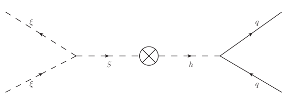
Figure 1: The Feynman diagram for the elastic scattering between a quark (q) and a PNGB.

Since all PNGBs are stable, we need to calculate three amplitudes for the direct detection cross section. However, due to the $O(3)$ symmetry of the interaction terms, the amplitude for the $\xi_{i}$-nucleon elastic scattering ($\xi_{i}n\to\xi_{i}n$) is proportional to $G_{i}$-nucleon elastic scattering amplitude and it is independent of $i$. In general, the interaction of the three-point terms pertinent to this interaction can be written as

$$\mathcal{L}_{\rm int}=-\frac{1}{2}\sum\limits_{i=1}^{3}\sum\limits_{j=1}^{3}\sum\limits_{k=1}^{2}Y^{(k)}_{ij}G_{i}G_{j}S_{k}\;.$$ (2.7)

But due to the $O(3)$ symmetry, we expect that

$$\mathcal{L}_{\rm int}=-\frac{1}{2}(G_{1}^{2}+G_{2}^{2}+G_{3}^{2})\,\sum\limits_{k=1}^{2}Y^{(k)}S_{k}=-\frac{1}{2}(\xi_{1}^{2}+\xi_{2}^{2}+\xi_{3}^{2})\,\sum\limits_{k=1}^{2}Y^{(k)}S_{k}\;.$$ (2.8)

From the potential 2.1 and the relations 2.4, we obtain

$$\mathcal{L}_{\rm int}=-\frac{1}{2}(\xi_{1}^{2}+\xi_{2}^{2}+\xi_{3}^{2})\left(\begin{matrix}\lambda_{H\Phi}\;v\\ -\dfrac{1}{v_{\Phi}}\left(\lambda_{H\Phi}v^{2}+4m_{\Phi_{22}}^{2}+2m_{\Phi_{22}}^{\prime\,2}\right)\end{matrix}\right)^{T}\left(\begin{matrix}h\\ \rho\end{matrix}\right)\;.$$ (2.9)

Since we are interested in the zero-momentum transfer limit, the propagator is proportional to the inverse of the mass-matrix $M_{S}^{2}$. Then the direct detection amplitude for all PNGBs (the Feynman diagram is shown in Fig. 1) becomes

$$A_{\rm DD}\sim\left(\begin{matrix}-\lambda_{H\Phi}v_{\Phi}v\\ \lambda_{H\Phi}v^{2}+4m_{\Phi_{22}}^{2}+2m_{\Phi_{22}}^{\prime\,2}\end{matrix}\right)^{T}\left(\begin{matrix}\lambda_{H\Phi}v^{2}+4m_{\Phi_{22}}^{2}+2m_{\Phi_{22}}^{\prime\,2}&\lambda_{H\Phi}v_{\Phi}v\\ \lambda_{H\Phi}v_{\Phi}v&-\lambda_{H}v^{2}\end{matrix}\right)\left(\begin{matrix}1\\ 0\end{matrix}\right)=0\;,$$ (2.10)

which concludes the proof of the claim that the DM-nucleon cross section vanishes at tree-level and zero momentum transfer. However, this only indicates that the direct detection cross section is “naturally suppressed”. In practice, loop corrections need to be included as well, since these effects could allow for a possible direct detection signal [32, 51, 52].

Generalization to $SU(N)$

It is straightforward to generalize the above result in the case where $\Phi$ is in the fundamental representation of a softly broken $SU(N)$ global symmetry, since the form of $V_{0}$ is the same as in eqs. (2.1), , with the soft breaking terms being

$$V_{\rm soft}=\sum\limits_{i=1}^{N}\sum\limits_{j=1}^{N}\Big{[}m_{\Phi\,ij}^{2}\Phi_{i}\Phi_{j}+{\rm h.c.}+m_{\Phi\,ij}^{\prime\,2}\Phi^{\dagger}_{i}\Phi_{j}\Big{]}\;,$$ (2.11)

where in analogy to $SU(2)$ $m_{\Phi\,ij}=m_{\Phi\,ji}$ and $m_{\Phi\,ij}^{\prime}=m_{\Phi\,ji}^{\prime\,*}$. Assuming that the $N^{\rm th}$ component of $\Phi$ develops a VEV, one can show that the minimization of the potential requires

$$m_{\Phi\,NN}^{2}\in\mathbb{R}$$

$$\mu_{H}^{2}=\lambda_{H}v^{2}+\lambda_{H\Phi}v_{\Phi}^{2}$$

$$m_{\Phi\,iN}^{2}=-\frac{m_{\Phi\,Ni}^{\prime\,2}}{2},\quad\forall i<N$$

$$\lambda_{\Phi}=-\frac{1}{v_{\Phi}^{2}}\left[\lambda_{H\Phi}v^{2}+4m_{\Phi_{NN}}^{2}+2m_{\Phi_{NN}}^{\prime\,2}\right]\;,$$ (2.12)

This results to $2N-1$ PNGBs, $\chi$, $\phi_{i}$ and $s_{i}$ with $i=1,2,\dots,N-1$, where, in complete analogy to the $SU(2)$ case, the interaction potential ($V_{0}$) becomes symmetric under $O(2N-1)$, which results to a $Z_{2}^{(\xi_{1})}\times Z_{2}^{(\xi_{2})}\dots\times Z_{2}^{(\xi_{2N-1})}$ symmetry for the entire potential. Therefore, all pseudo-Nambu-Goldstone bosons are stable particles. We also point out that the same arguments for the relic abundance of the $SU(2)$ case hold also in $SU(N)$. That is, in general the relic abundance should be $\Omega_{U(1)}h^{2}\lesssim\Omega_{SU(N)}h^{2}\lesssim(2N-1)\Omega_{U(1)}h^{2}$.

Returning to the discussion for the direct detection cross section, the pseudo-Nambu-Goldstone boson–nucleon interaction terms take the familiar form

$$\mathcal{L}_{\rm int}=-\frac{1}{2}\sum\limits_{i=1}^{2N-1}\xi_{i}^{2}\left(\begin{matrix}\lambda_{H\Phi}\;v\\ -\dfrac{1}{v_{\Phi}}\left(\lambda_{H\Phi}v^{2}+4m_{\Phi_{22}}^{2}+2m_{\Phi_{22}}^{\prime\,2}\right)\end{matrix}\right)^{T}\left(\begin{matrix}h\\ \rho\end{matrix}\right)\;,$$ (2.13)

Since the mass matrix $M_{S}^{2}$ is independent of $N$ (i.e. it is always given by eqs. (LABEL:eq:Mass_matrices-SU(2)), ), the amplitude for the process $\xi_{i}N\to\xi_{i}N$ at tree-level and zero momentum transfer, vanishes as in the $SU(2)$ case.

One should keep in mind that the cancellation takes place only if $\Phi$ is in the fundamental representation of $SU(N)$. It is not clear if $A_{\rm DD}$ would cancel if another (irreducible) representation of $\Phi$ was assumed, as there are additional interactions, corresponding to all the possible contractions of the $SU(N)$ indices. For example, for $N=2$ and $\Phi$ in the adjoint representation, there is an interaction term of the form

$$V_{\rm int}\sim|H|^{2}\sum\limits_{i,j,k,l}\epsilon^{il}\epsilon^{jk}\Phi_{ij}\Phi_{kl},$$

which can potentially change the mixing between the particles in a non-trivial way. Since the number of such interactions increases greatly with the dimension of each representation of $SU(N)$, it becomes hard to generalize. Thus, we postpone such analysis for the future. 

Beyond the tree-level approximation

Figure 2: An estimate of the 1-loop direct detection cross section eq. (2.14) for $\lambda=1$ (black line), $\lambda=0.7$ (dashed line), $\lambda=0.5$ (dashed-dotted line). The gray line corresponds to the upper limit as given by XENON1T [1].

So far, we have considered the direct detection cross section at the tree-level, which vanishes because of the PNGB nature of the DM particles, i.e. the approximate imposed symmetry. However, one expects that new interaction terms can be induced at the loop-level, from the contribution of the soft breaking terms. That is, one expects four-point symmetry breaking interaction terms (e.g. $|H|^{2}\Phi_{1}\Phi_{1}+\mathrm{h.c.}$) to be generated.  In this case, we expect a situation similar to ref. [32], with a typical loop-induced coupling $\lambda^{\prime}\sim\frac{\lambda^{2}}{(4\pi)^{2}}$ (multiplied by a function logarithmic in the mass parameters as in [32], which should vanish in the symmetric limit), and $\lambda^{2}$ proportional to a combination of $\lambda_{H\Phi}\lambda_{\Phi}+\lambda_{\Phi}^{2}$. That is, one expects for the direct detection cross section to be suppressed. An order of magnitude estimate can be deduced by assuming an interaction of the form (the tree level coupling cancels at zero momentum transfer, so we only show the loop-induced one here) $\mathcal{L}_{h\xi\xi}\sim\frac{\lambda^{2}}{(4\pi)^{2}}\,v\,h\,\xi^{2}$ ($\xi$ is a DM particle).  For such interactions, the spin-independent cross section is approximately [53]

$$\sigma_{SI}\sim 3.5\times 10^{-47}\left(\dfrac{100\,{\rm GeV}}{m_{\xi}}\right)^{2}\lambda^{4}\,{\rm cm}^{2}\,,$$ (2.14)

which for a moderate $\lambda\sim 0.5$ is below current limits (see fig. 2). Even for $\lambda=1$, this cross section is below the bounds, for most of the DM mass range. Note that since  eqs. (2.12),  suggests that $\lambda^{2}\sim\lambda_{H\Phi}\lambda_{\Phi}+\lambda_{\Phi}^{2}\sim\frac{\lambda_{H\Phi}^{2}v^{2}}{v_{\Phi}^{2}}\left[1-\left(\frac{v}{v_{\Phi}}\right)^{2}+\dots\right]$, such values of $\lambda$ are reasonable, assuming $v_{\Phi}>v,m_{\Phi\,NN}^{(\prime)}$. In principle, though, since we may have omitted important loop factors, one should calculate the relevant one-loop vertices ( or the complete 1-loop scalar potential as also stated in [32]), in order to have an accurate description of these interactions. Finally, one should keep in mind, that in the case of multi-component DM, each component contributes to the direct detection cross section according to its relative relic abundance [50]. This could mean more relaxed direct detection bounds (if the DM masses are separated), since for the various DM components, the DM-nucleon cross section should be rescaled as $\sigma^{i}_{SI}\approx\sigma_{SI}\times\frac{\Omega^{i}h^{2}}{\Omega^{tot}h^{2}}$ (for the $i^{\rm th}$ component).

Note on possible completions

The models presented here should not be considered UV-complete, since the origin of the global symmetries as well as the soft breaking terms are not known. That is, such models should be treated as low-energy limits of other, UV-complete, ones. Possible UV-completions, may include new gauge symmetries and a complicated spectrum of particles, so the explicitly broken symmetries may be manifested as approximate symmetries (as the so-called “custodial symmetry” in the SM [54]) in their low-energy limit. However, the structure of the low-energy models should be mostly unaffected, and any new effects induced by the completion, should be suppressed by some characteristic high-energy scale. In principle, such completion can induce decays of the DM particles, as well as other effects (e.g. tree-level DM interaction with the nucleons) not present in the low-energy model, but suppressed by the energy scale of the completion.  Such effects, though, can only be studied in a case-by-case manner provided a valid completion.

3 The $U(1)\times S_{2}$ case

In this section, we examine another case, which we denote as $U(1)\times S_{2}$. In this case, the SM is extended by two scalars ($S_{1,2}$) charged only under a softly broken global $U(1)$. For the desired cancellation to occur, we impose a permutation symmetry on $S_{1,2}$. As we will see, this symmetry provides a sufficient condition for the vanishing of the PNGB-nucleon cross section.

3.1 The cancellation mechanism for this model

The Potential

In the case of two scalars, each transforming as $S_{i}\to e^{-ia}S_{i}$, the $U(1)\times S_{2}$ symmetric potential, assuming that all parameters are real numbers (we shall call this assumption dark CP–invariance), is

$$V_{0} =-\frac{\mu_{H}^{2}}{2}\left|H\right|^{2}\,+\,\frac{\lambda_{H}^{2}}{2}\left|H\right|^{4}\,+\,\lambda_{HS_{1}}\left|H\right|^{2}\left(\left|S_{1}\right|^{2}+\left|S_{2}\right|^{2}\right)\,+\,\lambda_{HS_{2}}\left|H\right|^{2}\left(S_{1}S_{2}^{\dagger}+{\rm h.c.}\right)$$

$$\,-\,\frac{\mu_{S_{1}}^{2}}{2}\left(\left|S_{1}\right|^{2}+\left|S_{2}\right|^{2}\right)-\,\frac{\mu_{S_{2}}^{2}}{2}\left(S_{1}S_{2}^{\dagger}+{\rm h.c.}\right)\,+\,\frac{\lambda_{S_{1}}}{2}\left(\left|S_{1}\right|^{4}+\left|S_{2}\right|^{4}\right)\,+\,\frac{\lambda_{S_{2}}}{2}\left[(S_{1}S_{2}^{\dagger})^{2}+{\rm h.c.}\right]$$

$$+\,\lambda_{S}^{\prime}|S_{1}|^{2}|S_{2}|^{2}+\,c\,\left(S_{1}\,S_{2}^{\dagger}+S_{2}\,S_{1}^{\dagger}\right)\left(\left|S_{1}\right|^{2}+\left|S_{2}\right|^{2}\right)\;,$$ (3.1)

while the $S_{2}$-symmetric soft breaking potential is written as

$$V_{\rm soft}=-\frac{\mu_{S_{1}}^{\prime\,2}}{2}\left(S_{1}^{2}+S_{2}^{2}+\mathrm{h.c.}\right)\,-\,\mu_{S_{2}}^{\prime\,2}\left(S_{1}S_{2}+\mathrm{h.c.}\right)\;.$$ (3.2)

with the total potential given by $V=V_{0}+V_{\rm soft}$. In order to find the minimization conditions, we expand the fields around their VEVs

$$S_{1,2}=\frac{1}{\sqrt{2}}(v_{S}+s_{1,2}+i\,\chi_{1,2})\;,$$

$$H=\frac{1}{\sqrt{2}}\left(\begin{matrix}0\\ v+h\end{matrix}\right)\;,$$ (3.3)

where this particular choice of $\langle S_{1,2}\rangle$, ensures that the potential remains symmetric under simultaneous permutations of $\left(s\,,\,\chi\right)_{1}\leftrightarrow\left(s\,,\,\chi\right)_{2}$. Due to the permutation symmetry, there are only two independent stationary point conditions, which read

$$\mu_{H}^{2} = \lambda_{H}v^{2}+2v_{S}^{2}\left(\lambda_{HS_{1}}+\lambda_{HS_{2}}\right)\,,$$ (3.4)

$$\mu_{S_{1}}^{2} = v^{2}\left(\lambda_{HS_{1}}+\lambda_{HS_{2}}\right)\,-\,\left[\mu_{S_{2}}^{2}+2\left(\mu_{S_{1}}^{\prime\;2}+\mu_{S_{2}}^{\prime\;2}\right)\right]$$

$$+v_{S}^{2}\left(\lambda_{S_{1}}+\lambda_{S_{2}}+\lambda_{S}^{\prime}+4c\right)\,.$$

Spectrum of the CP–odd scalars

In order to calculate the direct detection amplitude, we first need to identify the PNGB. This can be done by diagonalizing the mass matrix of the CP–odd fields to its eigenvalues. Once the eigenvalues are found, one of them should vanish in the limit where the $U(1)$ is restored, which should correspond to the PNGB. From eqs. (3.1), , we obtain the mass matrix for the $\chi$’s

$$M_{\chi}^{2}=\left(\begin{matrix}-\frac{v^{2}\lambda_{HS_{2}}}{2}-v_{S}^{2}(\lambda_{S_{2}}+c)+2\mu_{S_{1}}^{\prime\;2}+\mu_{S_{2}}^{\prime\;2}+\frac{\mu_{S_{2}}^{2}}{2}&\frac{v^{2}\lambda_{HS_{2}}}{2}+v_{S}^{2}(\lambda_{S_{2}}+c)+\mu_{S_{2}}^{\prime\;2}-\frac{\mu_{S_{2}}^{2}}{2}\\ \frac{v^{2}\lambda_{HS_{2}}}{2}+v_{S}^{2}(\lambda_{S_{2}}+c)+\mu_{S_{2}}^{\prime\;2}-\frac{\mu_{S_{2}}^{2}}{2}&-\frac{v^{2}\lambda_{HS_{2}}}{2}-v_{S}^{2}(\lambda_{S_{2}}+c)+2\mu_{S_{1}}^{\prime\;2}+\mu_{S_{2}}^{\prime\;2}+\frac{\mu_{S_{2}}^{2}}{2}\end{matrix}\right),$$ (3.5)

from which we find the eigenvalues

$$m_{\xi_{1}}^{2} = 2(\mu_{S_{1}}^{\prime\,2}+\mu_{S_{2}}^{\prime\,2})$$

$$m_{\xi_{2}}^{2} = 2\mu_{S_{1}}^{\prime\;2}+\mu_{S_{2}}^{2}-v^{2}\lambda_{HS_{2}}-2v_{S}^{2}(\lambda_{S_{2}}+c)\;.$$ (3.6)

It is apparent that $m_{\xi_{1}}^{2}$ vanishes in the limit $\mu_{S_{1,2}}^{\prime\,2}\to 0$, thus the particle corresponding to this mass can be identified as the would-be Nambu-Goldstone boson of the $U(1)$, i.e. the PNGB of this model. The eigenstates corresponding to these masses are

$$\xi_{1}=\dfrac{1}{\sqrt{2}}(\chi_{1}+\chi_{2})\,,\,\xi_{2}=\dfrac{1}{\sqrt{2}}(\chi_{1}-\chi_{2})\;.$$ (3.7)

It is worth noting that the PNGB ($\xi_{1}$) is symmetric under $\chi_{1}\leftrightarrow\chi_{2}$. This property of the PNGB, will be proven helpful especially in the $N$-particle generalization of this model, since it will allow us to calculate the desired direct detection amplitude easily. The imposed dark CP–invariance can potentially keep both of the states $\xi_{1,2}$ stable, since there are only interactions involving even numbers of CP–odd particles, e.g. there is no $\xi_{1}\,h^{2}$ interaction term while the vertex $\xi_{1}^{2}\,h$ exists. However, since we are interested in the scenario where the DM particle is a PNGB, we need to impose an extra hierarchy condition, so that $\xi_{1}$ will be stable while $\xi_{2}$ will be able to decay. This condition is $m_{\xi_{1}}<m_{\xi_{2}}$, with their difference ($m_{\xi_{2}}-m_{\xi_{1}}$) at least larger than the mass of the lightest CP–even particle (e.g. $m_{\xi_{2}}-m_{\xi_{1}}>m_{H}\approx 125{\rm GeV}$ if the Higgs boson is the lightest one). This is not too restrictive, and it does not affect the vanishing of the PNGB-nucleon cross section, but it must be pointed out for the sake of completeness. Also, as in sec. 2, it seems reasonable that this model will be allowed by observations, at least close to the limit in which becomes similar to the $U(1)$ case. That said, however, since the parameter space is greater here, there should be room to accommodate all constraints (especially since the direct detection bounds are evaded).

The direct detection amplitude

The calculation of the quark-$\xi_{1}$ scattering amplitude is a relatively straightforward task. We just need to calculate the corresponding Feynman diagram (fig. 1). In fact, since we are interested in the zero momentum transfer limit, the ingredients that we need in order to show that the direct detection cross section vanishes, are the inverse of the mass matrix of the CP–even scalars and the three-point interaction of a pair of PNGBs with them (i.e. vertices of the form $\xi_{1}^{2}\,h$ and $\xi_{1}^{2}\,s_{1,2}$). The mass terms for the CP–even scalars can be written in a compact form as

$$\mathcal{L}_{\rm hs}=-\frac{1}{2}\Phi^{T}\,M^{2}_{\Phi}\,\Phi\;,$$ (3.8)

with $\Phi=\left(h,s_{1},s_{2}\right)^{T}$ and

$$M_{\Phi}^{2}=\left(\begin{matrix}v^{2}\lambda_{H}&vv_{S}(\lambda_{HS_{1}}+\lambda_{HS_{2}})&vv_{S}(\lambda_{HS_{1}}+\lambda_{HS_{2}})\\[2.84544pt] vv_{S}(\lambda_{HS_{1}}+\lambda_{HS_{2}})&\frac{2v_{S}^{2}(c+\lambda_{S_{1}})+\mu_{S_{2}}^{2}+2\mu_{S_{2}}^{\prime\,2}-\lambda_{HS_{2}}v^{2}}{2}&\frac{2v_{S}^{2}(3c+\lambda_{S_{2}}+\lambda_{S_{1}}^{\prime})+v^{2}\lambda_{HS_{2}}-\mu_{S_{2}}^{2}-2\mu_{S_{2}}^{\prime\,2}}{2}\\[2.84544pt] vv_{S}(\lambda_{HS_{1}}+\lambda_{HS_{2}})&\frac{2v_{S}^{2}(3c+\lambda_{S_{2}}+\lambda_{S_{1}}^{\prime})+v^{2}\lambda_{HS_{2}}-\mu_{S_{2}}^{2}-2\mu_{S_{2}}^{\prime\,2}}{2}&\frac{2v_{S}^{2}(c+\lambda_{S_{1}})+\mu_{S_{2}}^{2}+2\mu_{S_{2}}^{\prime\,2}-\lambda_{HS_{2}}v^{2}}{2}\end{matrix}\right)$$ (3.9)

Observing that only $h$ couples to SM fermions, we only need the following few terms of the inverse of $M_{\Phi}^{2}$

$$\left[M_{\Phi}^{2}\right]^{-1}_{11} \sim v_{S}^{2}\left(\lambda_{HS_{1}}+\lambda_{HS_{2}}+\lambda_{HS_{1}}^{\prime}+4c\right)$$ (3.10)

$$\left[M_{\Phi}^{2}\right]^{-1}_{i1} \sim\,-vv_{S}(\lambda_{HS_{1}}+\lambda_{HS_{2}})\,.$$

With the interaction term of the Lagrangian terms responsible for the $\xi_{1}$-nucleon elastic scattering being  

$$\mathcal{L}_{\rm int}=-\frac{1}{8}\xi_{1}^{2}\left(\begin{matrix}2v(\lambda_{HS_{1}}+\lambda_{HS_{2}})\\ v_{S}\left(\lambda_{HS_{1}}+\lambda_{HS_{2}}+\lambda_{HS_{1}}^{\prime}+4c\right)\\ v_{S}\left(\lambda_{HS_{1}}+\lambda_{HS_{2}}+\lambda_{HS_{1}}^{\prime}+4c\right)\end{matrix}\right)^{T}\left(\begin{matrix}h\\ s_{1}\\ s_{2}\end{matrix}\right),\;\;$$ (3.11)

we can show that the the amplitude for the $\xi_{1}$-nucleon elastic scattering vanishes. That is

$$A_{\rm DD}\sim\left(\begin{matrix}2v(\lambda_{HS_{1}}+\lambda_{HS_{2}})\\ v_{S}\left(\lambda_{HS_{1}}+\lambda_{HS_{2}}+\lambda_{HS_{1}}^{\prime}+4c\right)\\ v_{S}\left(\lambda_{HS_{1}}+\lambda_{HS_{2}}+\lambda_{HS_{1}}^{\prime}+4c\right)\end{matrix}\right)^{T}\left(\begin{matrix}v_{S}^{2}\left(\lambda_{HS_{1}}+\lambda_{HS_{2}}+\lambda_{HS_{1}}^{\prime}+4c\right)\\ -vv_{S}(\lambda_{HS_{1}}+\lambda_{HS_{2}})\\ -vv_{S}(\lambda_{HS_{1}}+\lambda_{HS_{2}})\end{matrix}\right)=0\;.$$ (3.12)

In analogy to the $SU(2)$ case, one again expects one-loop correction. This correction should be suppressed, with an induced coupling $\sim\frac{\lambda^{2}}{(4\pi)^{2}}$, with $\lambda$ combination of all couplings in this model. The case here is more involved, however, since the number of independent parameters is greater.

3.2 Generalization to $U(1)\times S_{N}$

As we saw in sec. 3.1, the cancellation mechanism holds when the model consists of two scalars under the assumption that the potential is symmetric under permutations of these scalars. This symmetry fixes the PNGB-$s_{1,2}$ interactions and the relevant components of $M_{\Phi}^{2}$ in such way that $A_{DD}$ vanishes. However, there is no guarantee that this also happens if we add more scalars, since more interaction terms are allowed. In this section, we investigate whether $A_{DD}$ vanishes in a model consisting of an arbitrary number of scalars. We denote this model as $U(1)\times S_{N}$, and it is a direct generalization of $U(1)\times S_{2}$ with $N$ number of scalars.

The Potential for $N$ Scalars

In the case of $N$ scalar fields, each transforming as $S_{i}\to e^{-ia}S_{i}$ (similarly to sec. 3.1), the $U(1)\times S_{N}$ symmetric potential, assuming again dark CP–invariance, can be written as

$$V_{0} =-\frac{\mu_{H}^{2}}{2}|H|^{2}\,+\,\frac{\lambda_{H}^{2}}{2}|H|^{4}-\sum\limits_{i,j}\frac{\mu_{S_{ij}}^{2}}{2}S_{i}S_{j}^{\dagger}+\sum\limits_{i,j}\frac{\lambda_{S_{ij}}}{2}(S_{i}S_{j}^{\dagger})^{2}+\sum\limits_{i,j}\frac{\lambda_{S_{ij}}^{\prime}}{2}|S_{i}|^{2}|S_{j}|^{2}$$ (3.13)

$$+\sum\limits_{i,j,k}c_{ijk}S_{i}S_{j}^{\dagger}|S_{k}|^{2}+\sum\limits_{i,j,k}c^{\prime}_{ijk}(S_{i}S_{j}S_{k}^{\dagger\,2}+{\rm h.c.})\,+\,\sum\limits_{i,j,k,l}d_{ijkl}S_{i}S_{j}S_{k}^{\dagger}S_{l}^{\dagger}$$

$$+\sum\limits_{i,j}\lambda_{HS_{ij}}|H|^{2}S_{i}S_{j}^{\dagger}\;,$$

where all the sums run over all scalars. This potential has some redundant terms, so we can set some of them to zero:

$$\lambda_{Sii}^{\prime} =0$$

$$c_{iik} =0$$

$$c_{iij}^{\prime} =c_{iji}^{\prime}=c_{ijj}^{\prime}=0$$

$$d_{iijk} =d_{ijik}=d_{ijki}=d_{ijjk}=d_{ijkj}=d_{ijkk}=0\;.$$ (3.14)

Furthermore, the permutation symmetry, dictates:

$$\mu^{2}_{S_{ij}}= \Big{\{}\begin{matrix}\mu^{2}_{S_{1}}&(i=j)\\ \mu^{2}_{S_{2}}&(i\neq j)\end{matrix}$$

$$\lambda_{S_{ij}}= \Big{\{}\begin{matrix}\lambda_{S_{1}}&(i=j)\\ \lambda_{S_{2}}&(i\neq j)\end{matrix}$$

$$\lambda_{HS_{ij}}= \Big{\{}\begin{matrix}\lambda_{HS_{1}}&(i=j)\\ \lambda_{HS_{2}}&(i\neq j)\end{matrix}$$

$$\lambda_{S_{ij}}^{\prime}= \lambda_{S}^{\prime}\hskip 19.91684pt(i\neq j)$$

$$c_{iji}=c_{jii}= c_{1}\;\hskip 19.91684pt(i\neq j)$$

$$c_{ijk}= c_{2}\hskip 22.76228pt(i\neq j\neq k)$$

$$c_{ijk}^{\prime}= c^{\prime}\hskip 24.18501pt(\ i\neq j\neq k)$$

$$d_{ijkl}= d\hskip 25.6073pt(i\neq j\neq k\neq l)\;.$$

As previously, we assume soft breaking of $U(1)$. That is, we add the following terms in the potential

$$V_{\rm soft}=-\sum\limits_{i,j}\frac{\mu_{Sij}^{\prime\,2}}{2}S_{i}S_{j}+\mathrm{h.c.}\;,$$ (3.16)

where, due to the $S_{N}$ symmetry, we have

$$\mu^{\prime\;2}_{S_{ij}}=\Big{\{}\begin{matrix}\mu^{\prime\;2}_{S_{1}}&(i=j)\\[4.26773pt] \mu^{\prime\;2}_{S_{2}}&(i\neq j)\end{matrix}$$ (3.17)

So, from eqs. (3.14), (3.2), (3.17), , the total potential becomes

$$V =-\dfrac{\mu_{H}^{2}}{2}|H|^{2}\,+\,\dfrac{\lambda_{H}^{2}}{2}|H|^{4}+\lambda_{HS_{1}}\sum\limits_{i}|H|^{2}|S_{i}|^{2}+\lambda_{HS_{2}}\sum\limits_{i\neq j}|H|^{2}S_{i}S_{j}^{\dagger}$$ (3.18)

$$-\dfrac{\mu_{S_{1}}^{2}}{2}\sum\limits_{i}|S_{i}|^{2}+\dfrac{\mu_{S_{2}}^{2}}{2}\sum\limits_{i\neq j}S_{i}S_{j}^{\dagger}+\dfrac{\lambda_{S_{1}}}{2}\sum\limits_{i}|S_{i}|^{4}+\dfrac{\lambda_{S_{2}}}{2}\sum\limits_{i\neq j}(S_{i}S_{j}^{\dagger})^{2}$$

$$+c_{1}\sum\limits_{i\neq j}\left(S_{i}S_{j}^{\dagger}|S_{j}|^{2}+S_{i}S_{j}^{\dagger}|S_{i}|^{2}\right)+c_{2}\sum\limits_{i\neq j\neq k}S_{i}S_{j}^{\dagger}|S_{k}|^{2}$$

$$+\lambda_{S}^{\prime}\sum\limits_{j>i}|S_{i}|^{2}|S_{j}|^{2}+c^{\prime}\sum\limits_{i\neq j\neq k}(S_{i}S_{j}S_{k}^{\dagger\,2}+{\rm h.c.})+d\sum\limits_{i\neq j\neq k\neq l}S_{i}S_{j}S_{k}^{\dagger}S_{l}^{\dagger}$$

$$-\frac{\mu_{S_{1}}^{\prime\,2}}{2}\sum\limits_{i}\left(S_{i}^{2}+\mathrm{h.c.}\right)-\mu_{S_{2}}^{\prime\,2}\sum\limits_{i}\left(S_{i}S_{j}+\mathrm{h.c.}\right)\;.$$

At this point, it becomes clear that the $S_{N}$ symmetry helps keeping the number of new free parameters relatively small.  This keeps the model as simple as possible, considering the potential large number of particles.

Similar to the previous, the scalars acquire VEVs

$$S_{i}=\frac{1}{\sqrt{2}}(v_{S}+s_{i}+i\,\chi_{i})\;,$$

$$H=\frac{1}{\sqrt{2}}\left(\begin{matrix}0\\ v+h\end{matrix}\right)\;,$$ (3.19)

where, again, we have assumed that the potential remains symmetric under $\left(\begin{matrix}s,\;\chi\end{matrix}\right)_{i}\leftrightarrow\left(\begin{matrix}s,\;\chi\end{matrix}\right)_{j}$ after SSB. From eqs. (3.18), (3.19), , we observe that there are only two independent stationary point conditions, due to the $S_{N}$ symmetry, (similar to 3.1), which are

$$\mu_{H}^{2} = \lambda_{H}v^{2}+Nv_{S}^{2}\left[\lambda_{HS_{1}}+(N-1)\lambda_{HS_{2}}\right]\;,$$ (3.20)

$$\mu_{S_{1}}^{2} = v^{2}\left[\lambda_{HS_{1}}+(N-1)\lambda_{HS_{2}}\right]-\left[2\mu_{S_{1}}^{\prime\;2}+(N-1)(\mu_{S_{2}}^{2}+2\mu_{S2}^{\prime\;2})\right]$$

$$+ v_{S}^{2}\Big{[}\lambda_{S_{1}}+(N-1)(\lambda_{S_{2}}+\lambda_{S}^{\prime}+4c_{1})+2(N-1)(N-2)(c_{2}+2c^{\prime})$$

$$+ 2(N-1)(N-2)(N-3)d\Big{]}\;.$$

These conditions further reduce the number of new parameters by one, i.e. the maximum number of new parameters introduced is $12$ for $N\geq 4$ (for $N=2$ and $3$ these are $9$ and $11$, respectively).

Spectrum of the CP–odd scalars

As in sec. 3.1, our next step is to find which mass eigenstate corresponds to the PNGB. To do so, we first have to find the mass matrix ($M_{\chi}^{2}$) for the CP–odd scalars. Since the CP–odd and CP–even scalars do not mix (due to the dark CP–invariance), their mass terms are symmetric under permutations of the $\chi$’s. As a result, there are only two different entries in the mass matrix for $\chi$’s, the diagonal, $\left(M_{\chi}^{2}\right)_{ii}$, and the off diagonal, $\left(M_{\chi}^{2}\right)_{ij}$, ones. After some algebra, one can show that

$$[M_{\chi}^{2}]_{ii} =-v^{2}(N-1)\frac{\lambda_{HS_{2}}}{2}+2\mu_{S_{1}}^{\prime\;2}+\frac{1}{2}(N-1)(2\mu_{S_{2}}^{\prime\;2}+\mu_{S_{2}}^{2})$$

$$-v_{S}^{2}\Big{[}(N-1)(\lambda_{S_{2}}+c_{1})+\frac{1}{2}(N-1)(N-2)(c_{2}+6c^{\prime})$$ (3.21)

$$+(N-1)(N-2)(N-3)\Big{]}\;,$$

$$[M_{\chi}^{2}]_{ij} =\frac{2\left(\mu_{S_{1}}^{\prime\;2}+(N-1)\mu_{S_{2}}^{\prime\;2}\right)-[M_{\chi}^{2}]_{ii}}{(N-1)}\qquad\qquad\qquad\qquad\qquad\qquad\text{ for $i\neq j$}\;.$$

The eigenvalues of this matrix are

$$m_{\xi_{1}}^{2} =[M_{\chi}^{2}]_{ij}+(N-1)\;[M_{\chi}^{2}]_{ii}=2\left(\mu_{S_{1}}^{\prime\;2}+(N-1)\mu_{S_{2}}^{\prime\;2}\right)$$ (3.22)

$$m_{\xi_{i}}^{2} =[M_{\chi}^{2}]_{ii}-[M_{\chi}^{2}]_{ij}\hskip 199.16928pt\text{ for }i=2,3...N\;.$$ (3.23)

The first ($m_{\xi_{1}}^{2}$) corresponds to the particle $\xi_{1}$, which is the PNGB ($m_{\xi_{1}}^{2}\to 0$ as $\mu_{S_{1,2}}^{\prime\;2}\to 0$), while the other particles ($\xi_{2,3,\dots,N}$) are degenerate with mass $m_{\xi_{2}}=m_{\xi_{3}}=\dots=m_{\xi_{N}}$. As it turns out (in analogy to sec. 3.1), the PNGB is the $S_{N}$-symmetric state

$$\xi_{1}=\frac{1}{\sqrt{N}}\sum\limits_{i=1}^{N}\chi_{i}\;,$$ (3.24)

where the others (not relevant to our discussion) can be found from orthonormality conditions. We also note again that some hierarchy conditions should be imposed in order for the PNGB to be the DM particle.

The Cancellation of the Direct Detection Cross Section

Again the ingredients that we need in order to show that the direct detection cross section vanishes, are the inverse of the mass matrix for the real part of the scalars and the interaction of a pair of pseudo-Nambu-Goldstone particles with them (i.e. $\xi_{1}^{2}-h,\,s_{i}$).

As usual the mass terms for the CP–even scalars can be written in a compact form as

$$\mathcal{L}_{\rm hs}=-\frac{1}{2}\Phi^{T}\,M^{2}_{\Phi}\,\Phi\;,$$ (3.25)

with $\Phi=\left(\begin{matrix}h\ s_{1}\ s_{2}\dots\end{matrix}\right)^{T}$ and

$$[M^{2}_{\Phi}]_{11} =v^{2}\lambda_{H}\;,$$

$$[M^{2}_{\Phi}]_{1i} =(M^{2}_{hs})_{i1}=v\,v_{S}\left[\lambda_{HS_{1}}+(N-1)\lambda_{HS_{2}}\right] \text{ for }i>1\;,$$

$$[M^{2}_{\Phi}]_{ii} =-v^{2}(N-1)\frac{\lambda_{HS_{2}}}{2}+\frac{N-1}{2}(\mu_{S_{2}}^{2}+\mu_{S_{2}}^{\prime\,2})+v_{S}^{2}\Big{[}\lambda_{S_{1}}$$ (3.26)

$$+(N-1)c_{1}-\frac{1}{2}(N-1)(N-2)(c_{2}+2c_{2}^{\prime})$$

$$-(N-1)(N-2)(N-3)d\Big{]} \text{ for }i>1\;,$$

$$[M^{2}_{\Phi}]_{ij} =v^{2}\frac{\lambda_{HS_{2}}}{2}-\frac{1}{2}(\mu_{S_{2}}^{2}+\mu_{S_{2}}^{\prime\,2})+v_{S}^{2}\Big{[}(\lambda_{S_{2}}+\lambda_{S_{1}}^{\prime}+3c_{1})$$

$$+\frac{5}{2}(N-2)(c_{2}+2c_{2}^{\prime})+3(N-2)(N-3)d\Big{]} \text{ for }i,j>1\;.$$

The interaction term of the Lagrangian which is responsible for the $\xi_{1}-N$ elastic scattering is

$$\mathcal{L}_{\rm int} =-\frac{1}{4N}\xi_{1}^{2}\left(\begin{matrix}Y_{\xi h},Y_{\xi s},Y_{\xi s},\dots\end{matrix}\right)\left(\begin{matrix}h\\ s_{1}\\ s_{2}\\ \vdots\end{matrix}\right)\;,$$ (3.27)

with

$$Y_{\xi\,h} =vN\left[\lambda_{HS_{1}}+(N-1)\lambda_{HS_{2}}\right]$$ (3.28)

$$Y_{\xi\,s} =v_{S}\Big{\{}\lambda_{S_{1}}+(N-1)\left[\lambda_{S_{2}}+\lambda_{S_{1}}^{\prime}+4c_{1}+2(N-2)\left(c_{2}+2c^{\prime}+(N-3)d\right)\right]\Big{\}}\,.$$ (3.29)

Again, the propagator (i.e. the inverse of the $s-h$ mass matrix) should be multiplied by a column vector $\sim\delta_{1i}$ (since only $h$ interacts with SM fermions), so the elements of the inverse of $M_{hs}^{2}$ relevant to the DM-nucleon interaction are

$$[M_{\Phi}^{2}]^{-1}_{11} \sim[M_{\Phi}^{2}]_{22}+(N-1)[M_{\Phi}^{2}]_{23}\;.$$

$$[M_{\Phi}^{2}]^{-1}_{i1} \sim-[M_{\Phi}^{2}]_{12}$$ (3.30)

As in sec. 3.1, the Feynman diagram for the elastic PNGB-quark scattering is given fig. 1, with an amplitude proportional to

$$A_{\rm DD}\sim\left(\begin{matrix}Y_{\xi h},Y_{\xi s},Y_{\xi s},\dots\end{matrix}\right)\left(\begin{matrix}[M_{\Phi}^{2}]^{-1}_{11}\\ [M_{\Phi}^{2}]^{-1}_{i1}\\ [M_{\Phi}^{2}]^{-1}_{i1}\\ \vdots\end{matrix}\right)\;,$$ (3.31)

which, from eqs. (3.26), (3.27), (3.30), , can be shown that vanishes.

A Note on the dark CP–invariance

$N$	#phases
1	1
2	3
$\geq 3$	$3+\frac{1}{2}N(N-1)$

Table 1: Number of phases for various values of $N$

In ref. [32] it was argued that the $U(1)$ case is invariant under $S\to S^{\dagger}$, because there is one phase which can be absorbed by $S$. This natural symmetry of the model guarantees that the imaginary part of $S$ (the CP–odd scalar) always interact in pairs and as a result it is stable. However, when the scalar sector consists of a larger number of particles, it is not possible to absorb all phases to the scalars, as shown in Table 1. Therefore, in order to guarantee the stability of the DM particle $\xi_{1}$, we have to assume that all parameters are real on top of the $S_{N}$ symmetry.

4 Conclusion and future direction

Inspired by an Abelian model which introduced a natural mechanism for the vanishing of the direct detection cross section, we have expanded the discussion on the explanation of the smallness of the DM direct detection cross section.

The first case under study (sec. 2) was a softly broken $SU(2)$ global symmetry. In this, we assumed that there is a doublet scalar (singlet under the SM gauge symmetry), which acquires a VEV. We showed that the resulting pseudo-Nambu-Goldstone bosons are all DM candidates, due to a remaining discrete symmetry that keeps them stable. We also showed that the DM–neucleon interaction vanishes. Then, we argued that this case can be generalized in a straightforward fashion to an $SU(N)$ symmetry, leading to the same result, i.e. vanishing of the DM–neucleon interaction.

Then in sec. 3.2 we examined the $U(1)\times S_{N}$ global symmetry, with $U(1)$ being softly broken, where we extended the scalar sector by adding $N$ scalars, charged only under a global $U(1)$. Assuming a dark CP–invariance, we calculated the form of the mass matrices and three-point interactions relevant to the pseudo-Nambu-Goldstone–nucleon interaction, which turned out to vanish.

A parameter space analysis of some simple cases (e.g. $U(1)\times S_{2}$ or $SU(2)$), will help us identify potential discovery channels at the LHC and astrophysical observations [48, 34]. Also, a calculation of 1-loop corrections will give us with precision the direct detection cross section, which can further be used to probe (or even exclude) the models discussed in this work. In addition, since the cases at hand should be treated as low-energy limits of complete models, an interesting direction would be to determine possible completions. These, can induce (parametrically or energetically suppressed [32, 34]) DM-nucleon interactions at the tree-level as well as decays of the PNGBs, allowing for a rich phenomenology, and connection of the DM problem with other open issues in particle physics (e.g. lepton number violation and neutrino masses [55]). Furthermore, there are some cases that we did not consider (i.e. the general irrep of the $SU(N)$ case), a study of other simple considerations (e.g. $SU(2)$-triplet) can be insightful, and help us identify similar classes of models. However, since we were only interested in furthering the discussion on the suppression of the DM-nucleon interaction, with a focus on simple realizations, we postpone these for a later project.

References

• [1] XENON Collaboration, E. Aprile et al., Dark Matter Search Results from a One Ton-Year Exposure of XENON1T, Phys. Rev. Lett. 121 (2018), no. 11 111302, [arXiv:1805.12562].
• [2] G. Bertone and D. Hooper, History of dark matter, Rev. Mod. Phys. 90 (2018), no. 4 045002, [arXiv:1605.04909].
• [3] M. Pospelov, A. Ritz, and M. B. Voloshin, Secluded WIMP Dark Matter, Phys. Lett. B662 (2008) 53–61, [arXiv:0711.4866].
• [4] M. Pospelov and A. Ritz, Astrophysical Signatures of Secluded Dark Matter, Phys. Lett. B671 (2009) 391–397, [arXiv:0810.1502].
• [5] D. Pappadopulo, J. T. Ruderman, and G. Trevisan, Dark matter freeze-out in a nonrelativistic sector, Phys. Rev. D94 (2016), no. 3 035005, [arXiv:1602.04219].
• [6] H. Mebane, N. Greiner, C. Zhang, and S. Willenbrock, Constraints on Electroweak Effective Operators at One Loop, Phys. Rev. D88 (2013), no. 1 015028, [arXiv:1306.3380].
• [7] M. A. Fedderke, J.-Y. Chen, E. W. Kolb, and L.-T. Wang, The Fermionic Dark Matter Higgs Portal: an effective field theory approach, JHEP 08 (2014) 122, [arXiv:1404.2283].
• [8] J. Hisano, D. Kobayashi, N. Mori, and E. Senaha, Effective Interaction of Electroweak-Interacting Dark Matter with Higgs Boson and Its Phenomenology, Phys. Lett. B742 (2015) 80–85, [arXiv:1410.3569].
• [9] S. Matsumoto, S. Mukhopadhyay, and Y.-L. S. Tsai, Effective Theory of WIMP Dark Matter supplemented by Simplified Models: Singlet-like Majorana fermion case, Phys. Rev. D94 (2016), no. 6 065034, [arXiv:1604.02230].
• [10] A. Dedes, D. Karamitros, and V. C. Spanos, Effective Theory for Electroweak Doublet Dark Matter, Phys. Rev. D94 (2016), no. 9 095008, [arXiv:1607.05040].
• [11] J. Yepes, Top partners tackling vector dark matter, arXiv:1811.06059.
• [12] C. Cheung, L. J. Hall, D. Pinner, and J. T. Ruderman, Prospects and Blind Spots for Neutralino Dark Matter, JHEP 05 (2013) 100, [arXiv:1211.4873].
• [13] S. Banerjee, S. Matsumoto, K. Mukaida, and Y.-L. S. Tsai, WIMP Dark Matter in a Well-Tempered Regime: A case study on Singlet-Doublets Fermionic WIMP, JHEP 11 (2016) 070, [arXiv:1603.07387].
• [14] T. Han, H. Liu, S. Mukhopadhyay, and X. Wang, Dark Matter Blind Spots at One-Loop, arXiv:1810.04679.
• [15] L. Heurtier and D. Teresi, Dark matter and observable lepton flavor violation, Phys. Rev. D94 (2016), no. 12 125022, [arXiv:1607.01798].
• [16] A. Dedes, D. Karamitros, and A. Pilaftsis, Radiative Light Dark Matter, Phys. Rev. D95 (2017), no. 11 115037, [arXiv:1704.01497].
• [17] S. Knapen, T. Lin, and K. M. Zurek, Light Dark Matter: Models and Constraints, Phys. Rev. D96 (2017), no. 11 115021, [arXiv:1709.07882].
• [18] L. Darmé, S. Rao, and L. Roszkowski, Light dark Higgs boson in minimal sub-GeV dark matter scenarios, JHEP 03 (2018) 084, [arXiv:1710.08430].
• [19] M. Dutra, M. Lindner, S. Profumo, F. S. Queiroz, W. Rodejohann, and C. Siqueira, MeV Dark Matter Complementarity and the Dark Photon Portal, JCAP 1803 (2018) 037, [arXiv:1801.05447].
• [20] P. Foldenauer, Let there be Light Dark Matter: The gauged $U(1)_{L_{\mu}-L_{\tau}}$ case, arXiv:1808.03647.
• [21] S. Matsumoto, Y.-L. S. Tsai, and P.-Y. Tseng, Light Fermionic WIMP Dark Matter with Light Scalar Mediator, arXiv:1811.03292.
• [22] L. J. Hall, K. Jedamzik, J. March-Russell, and S. M. West, Freeze-In Production of FIMP Dark Matter, JHEP 03 (2010) 080, [arXiv:0911.1120].
• [23] A. Dedes, I. Giomataris, K. Suxho, and J. D. Vergados, Searching for Secluded Dark Matter via Direct Detection of Recoiling Nuclei as well as Low Energy Electrons, Nucl. Phys. B826 (2010) 148–173, [arXiv:0907.0758].
• [24] R. Essig, T. Volansky, and T.-T. Yu, New Constraints and Prospects for sub-GeV Dark Matter Scattering off Electrons in Xenon, Phys. Rev. D96 (2017), no. 4 043017, [arXiv:1703.00910].
• [25] J. A. Evans, Detecting Hidden Particles with MATHUSLA, Phys. Rev. D97 (2018), no. 5 055046, [arXiv:1708.08503].
• [26] J. L. Feng, I. Galon, F. Kling, and S. Trojanowski, ForwArd Search ExpeRiment at the LHC, Phys. Rev. D97 (2018), no. 3 035001, [arXiv:1708.09389].
• [27] FASER Collaboration, A. Ariga et al., FASER’s Physics Reach for Long-Lived Particles, arXiv:1811.12522.
• [28] DarkSide Collaboration, P. Agnes et al., Constraints on Sub-GeV Dark-Matter–Electron Scattering from the DarkSide-50 Experiment, Phys. Rev. Lett. 121 (2018), no. 11 111303, [arXiv:1802.06998].
• [29] LDMX Collaboration, T. Åkesson et al., Light Dark Matter eXperiment (LDMX), arXiv:1808.05219.
• [30] A. Dedes and D. Karamitros, Doublet-Triplet Fermionic Dark Matter, Phys. Rev. D89 (2014), no. 11 115002, [arXiv:1403.7744].
• [31] G. Arcadi, C. Gross, O. Lebedev, Y. Mambrini, S. Pokorski, and T. Toma, Multicomponent Dark Matter from Gauge Symmetry, JHEP 12 (2016) 081, [arXiv:1611.00365].
• [32] C. Gross, O. Lebedev, and T. Toma, Cancellation Mechanism for Dark-Matter–Nucleon Interaction, Phys. Rev. Lett. 119 (2017), no. 19 191801, [arXiv:1708.02253].
• [33] R. Balkin, M. Ruhdorfer, E. Salvioni, and A. Weiler, Dark matter shifts away from direct detection, JCAP 1811 (2018), no. 11 050, [arXiv:1809.09106].
• [34] T. Alanne, M. Heikinheimo, V. Keus, N. Koivunen, and K. Tuominen, Direct and indirect probes of Goldstone dark matter, arXiv:1812.05996.
• [35] V. Silveira and A. Zee, SCALAR PHANTOMS, Phys. Lett. 161B (1985) 136–140.
• [36] J. McDonald, Gauge singlet scalars as cold dark matter, Phys. Rev. D50 (1994) 3637–3649, [hep-ph/0702143].
• [37] C. P. Burgess, M. Pospelov, and T. ter Veldhuis, The Minimal model of nonbaryonic dark matter: A Singlet scalar, Nucl. Phys. B619 (2001) 709–728, [hep-ph/0011335].
• [38] Y. G. Kim and K. Y. Lee, The Minimal model of fermionic dark matter, Phys. Rev. D75 (2007) 115012, [hep-ph/0611069].
• [39] L. Lopez-Honorez, T. Schwetz, and J. Zupan, Higgs portal, fermionic dark matter, and a Standard Model like Higgs at 125 GeV, Phys. Lett. B716 (2012) 179–185, [arXiv:1203.2064].
• [40] A. Freitas, S. Westhoff, and J. Zupan, Integrating in the Higgs Portal to Fermion Dark Matter, JHEP 09 (2015) 015, [arXiv:1506.04149].
• [41] A. Karam and K. Tamvakis, Dark matter and neutrino masses from a scale-invariant multi-Higgs portal, Phys. Rev. D92 (2015), no. 7 075010, [arXiv:1508.03031].
• [42] G. Arcadi, C. Gross, O. Lebedev, S. Pokorski, and T. Toma, Evading Direct Dark Matter Detection in Higgs Portal Models, Phys. Lett. B769 (2017) 129–133, [arXiv:1611.09675].
• [43] J. A. Casas, D. G. Cerdeño, J. M. Moreno, and J. Quilis, Reopening the Higgs portal for single scalar dark matter, JHEP 05 (2017) 036, [arXiv:1701.08134].
• [44] L. Lopez Honorez, M. H. G. Tytgat, P. Tziveloglou, and B. Zaldivar, On Minimal Dark Matter coupled to the Higgs, JHEP 04 (2018) 011, [arXiv:1711.08619].
• [45] A. Filimonova and S. Westhoff, Long live the Higgs portal!, arXiv:1812.04628.
• [46] S. Bhattacharya, B. Melić, and J. Wudka, Pionic Dark Matter, JHEP 02 (2014) 115, [arXiv:1307.2647].
• [47] A. Semenov, LanHEP — A package for automatic generation of Feynman rules from the Lagrangian. Version 3.2, Comput. Phys. Commun. 201 (2016) 167–170, [arXiv:1412.5016].
• [48] K. Huitu, N. Koivunen, O. Lebedev, S. Mondal, and T. Toma, Probing pseudo-Goldstone dark matter at the LHC, arXiv:1812.05952.
• [49] G. Belanger, K. Kannike, A. Pukhov, and M. Raidal, Impact of semi-annihilations on dark matter phenomenology - an example of $Z_{N}$ symmetric scalar dark matter, JCAP 1204 (2012) 010, [arXiv:1202.2962].
• [50] A. DiFranzo and G. Mohlabeng, Multi-component Dark Matter through a Radiative Higgs Portal, JHEP 01 (2017) 080, [arXiv:1610.07606].
• [51] D. Azevedo, M. Duch, B. Grzadkowski, D. Huang, M. Iglicki, and R. Santos, One-loop contribution to dark-matter-nucleon scattering in the pseudo-scalar dark matter model, JHEP 01 (2019) 138, [arXiv:1810.06105].
• [52] K. Ishiwata and T. Toma, Probing pseudo Nambu-Goldstone boson dark matter at loop level, JHEP 12 (2018) 089, [arXiv:1810.08139].
• [53] E. Hardy, Higgs portal dark matter in non-standard cosmological histories, JHEP 06 (2018) 043, [arXiv:1804.06783].
• [54] P. Sikivie, L. Susskind, M. B. Voloshin, and V. I. Zakharov, Isospin Breaking in Technicolor Models, Nucl. Phys. B173 (1980) 189–207.
• [55] F. S. Queiroz and K. Sinha, The Poker Face of the Majoron Dark Matter Model: LUX to keV Line, Phys. Lett. B735 (2014) 69–74, [arXiv:1404.1400].