Random graphs with given vertex degrees and switchings

Abstract.

Random graphs with a given degree sequence are often constructed using the configuration model, which yields a random multigraph. We may adjust this multigraph by a sequence of switchings, eventually yielding a simple graph. We show that, assuming essentially a bounded second moment of the degree distribution, this construction with the simplest types of switchings yields a simple random graph with an almost uniform distribution, in the sense that the total variation distance is $o(1)$. This construction can be used to transfer results on distributional convergence from the configuration model multigraph to the uniform random simple graph with the given vertex degrees. As examples, we give a few applications to asymptotic normality. We show also a weaker result yielding contiguity when the maximum degree is too large for the main theorem to hold.

1. Introduction

We consider random graphs with vertex set $[n]:=\{1,\dots,n\}$ and a given degree sequence $\mathbf{d}=\bigl{(}d_{1},\dots,d_{n}\bigr{)}$. In particular, we define $G(n,\mathbf{d})$ to be the random (simple) graph with degree sequence $\mathbf{d}$ chosen uniformly at random among all such graphs. We will consider asymptotic results as ${n\to\infty}$, where the degree sequence $\mathbf{d}=\mathbf{d}_{n}=(d_{i}^{(n)})_{1}^{n}$ depends on $n$, but usually we omit $n$ from the notation.

The standard methods to constuct a random graph with a given degree sequence begin with the configuration model, which was introduced by Bollobás [7]. (See [6; 31] for related models and arguments.) As is well-known, this method yields a random multigraph, which we denote by $G^{*}(n,\mathbf{d})$, with the given degree sequence $\mathbf{d}$; see Section 3.1. This random multigraph may contain loops and multiple edges; however, in the present paper (as in many others), we will consider asymptotic results as ${n\to\infty}$, where $\mathbf{d}=\mathbf{d}_{n}$ satisfies (at least)

$$\sum_{i=1}^{n}d_{i}=\Theta(n), \sum_{i=1}^{n}d_{i}^{2}=O(n),$$ (1.1)

and then (see e.g. the proof of Lemma 4.1) the expected number of loops and multiple edges is $O(1)$, which might seem insignificant when $n$ is large. (Recall that $\Theta(n)$ means a number in the interval $[cn,Cn]$ for some constants $c,C>0$.)

In fact, we are mainly interested in the more regular case where, as ${n\to\infty}$,

$$\frac{1}{n}\sum_{i=1}^{n}d_{i}\to\mu, \frac{1}{n}\sum_{i=1}^{n}d_{i}^{2}\to\mu_{2}$$ (1.2)

for some $\mu,\mu_{2}\in(0,\infty)$. Obviously, (1.2) implies (1.1). Conversely, if (1.1) holds, then there is always a subsequence satisfying (1.2). It follows, see Section 4.4 for details, that for our purposes (1.1) and (1.2) are essentially equivalent. We will thus use the more general (1.1) in the theorems.

In some applications, the random multigraph $G^{*}(n,\mathbf{d})$ may be at least as good as the simple graph $G(n,\mathbf{d})$. For example, this may be the case in an application where the random graph is intended to be an approximation of an unknown graph “in real life”; then the multigraph model may be just as good as an approximation. On the other hand, if we, as is often the case, really want a random simple graph (i.e., no loops or multiple edges), then there are several ways to proceed.

The standard method, at least in the sparse case studied in the present paper, is to condition $G^{*}(n,\mathbf{d})$ on the event that it is a simple graph; it is a fundamental fact of the configuration model construction (implicit in [7]) that this yields a random simple graph $G(n,\mathbf{d})$ with the uniform distribution over all graphs with the given degree sequence. This method has been very successful in many cases. In particular, under the condition (1.1) on $\mathbf{d}$,

$$\liminf_{n\to\infty}\operatorname{\mathbb{P}{}}\bigl{(}G^{*}(n,\mathbf{d})\text{ is simple}\bigr{)}>0,$$ (1.3)

see e.g. [16; 18], and then any result on convergence in probability for $G^{*}(n,\mathbf{d})$ immediately transfers to $G(n,\mathbf{d})$. (See also Bollobás and Riordan [8], where this method is used, with more complicated arguments, also in cases with $\operatorname{\mathbb{P}{}}\bigl{(}G^{*}(n,\mathbf{d})\text{ is simple}\bigr{)}\to 0$.) However, as is also well-known, results on convergence in distribution do not transfer so easily, and further arguments are needed. (See [21], [29], [19] for examples where this has succeded, with more or less complicated extra arguments.)

Another method to create a simple graph from $G^{*}(n,\mathbf{d})$ is to erase all loops and merge any set of parallel edges into a single edge. This creates a simple random graph, but typically its degree sequence is not exactly the given sequence $\mathbf{d}$. Nevertheless, this erased configuration model may be as useful as $G^{*}(n,\mathbf{d})$ in some applications. This construction is studied in Britton, Deijfen and Martin-Löf [9] and van der Hofstad [15, Section 3], but will not be considered further in the present paper where we insist on the degree sequence being exactly $\mathbf{d}$.

In the present paper, we consider a different method, where we also adjust $G^{*}(n,\mathbf{d})$ to make it simple, but this time we keep the degree sequence $\mathbf{d}$ exact by using switchings instead of erasing. More precisely, we process the loops and multiple edges in $G^{*}(n,\mathbf{d})$ one by one. For each such bad edge, we chose another edge, uniformly at random, and switch the endpoints of these two edges, thus replacing them by another pair of edges. See Section 3.2 for details. Assuming (1.1), this typically gives a simple graph after a single pass through the bad edges (Theorem 3.2); if not, we repeat until a simple graph is obtained. We denote the resulting graph by $\widehat{G}(n,\mathbf{d})$ and call it the switched configuration model. The idea to use switchings in this context goes back to McKay [25] for the closely related problem of counting simple graphs with a given degree sequence (assuming $\max d_{i}=O(n^{1/4})$, but not (1.1)), and was made explicit for generating $G(n,\mathbf{d})$ by McKay and Wormald [26] (using somewhat different switchings). See the survey by Wormald [33] for further uses of switchings. Recent refinements of the method, extending it to larger classes of degree sequences by employing more types of switchings, are given in Gao and Wormald [10, 11, 12]. We will not use these recent refinements (that have been developed to handle also rather dense graphs); instead we focus on the simple case when (1.1) holds and only a few switchings are needed; we also use only the oldest and simplest types of switchings, used already by McKay [25] (called simple switchings in [33]). Although the switching method for this case has been known for a long time, it seems to have been somewhat neglected. Our purpose is to show that the switching method is powerful also in this case, and that it complements the conditioning method discussed above for the purpose of proving asymptotic results for $G(n,\mathbf{d})$.

Remark 1.1.

From the point of view of constructing a random simple graph with given degree sequence by simulation, the standard approach using conditioning means that we sample the multigraph $G^{*}(n,\mathbf{d})$; if it happens to be simple, we accept it, and otherwise we discard it completely and start again, repeating until a simple graph is found. (See e.g. [32].) The approach in the present paper is instead to keep most of the multigraph even when it is not simple, and resample only a few edges. The disadvantage is that the result $\widehat{G}(n,\mathbf{d})$ is not perfectly uniformly random, but Theorem 2.1 below shows that is a good approximation, and asymptotically correct. The advantage is that $\widehat{G}(n,\mathbf{d})$ typically does not differ much from $G^{*}(n,\mathbf{d})$, and thus we often can show estimates of the type (2.10) in Corollary 2.3 below.

Remark 1.2.

In e.g. [26; 11; 12], an exactly uniformly distributed simple graph (i.e., $G(n,\mathbf{d})$) is constructed by combining switchings with rejection sampling, meaning that we may, with some carefully calculated probabilities, abort the construction and restart. (Cf. the conditioning method where, as discussed in Remark 1.1, we restart as soon as anything is wrong, instead of trying to fix it by switchings.) Our focus is not on actual concrete construction of instances of $G(n,\mathbf{d})$ by simulation, but rather to have a method of construction that can be used theoretically to study properties of $G(n,\mathbf{d})$, and for our purposes the approximate uniformity given by Theorem 2.1 is good enough. (And better, since the method is simpler.)

Remark 1.3.

Switchings have also recently been used (in a different way) by Athreya and Yogeshwaran [1] to prove asymptotic normality for statistics of $G^{*}(n,\mathbf{d})$ (in a subcritical case) using martingale methods.

Remark 1.4.

For convenience, we state the results for a sequence $\mathbf{d}_{n}$ of degree sequences where $\mathbf{d}_{n}$ has length (number of vertices) $n$. More generally, one might consider a subsequence, or other sequences of degree sequences $\mathbf{d}_{j}$ with lengths $n_{j}\to\infty$. This will be used in the proofs, see Section 4.4.

The main results are stated in Section 2, and proved in Sections 4–7. A few applications are given in Section 8.

2. Notation and main results

2.1. Some notation

Unspecified limits are as ${n\to\infty}$; w.h.p. (with high probability) means with probability tending to 1 as ${n\to\infty}$. $\overset{\mathrm{d}}{\longrightarrow}$ and $\overset{\mathrm{p}}{\longrightarrow}$ denote convergence in distribution and probability, respectively.

If $X_{n}$ are random variables and $a_{n}$ are positive numbers, then $X_{n}=O_{\mathrm{p}}(a_{n})$ means $\lim_{K\to\infty}\sup_{n}\operatorname{\mathbb{P}{}}(|X_{n}|>Ka_{n})=0$, and $X_{n}=o_{\mathrm{p}}(a_{n})$ means $\sup_{n}\operatorname{\mathbb{P}{}}(|X_{n}|>\varepsilon a_{n})=0$ for every $\varepsilon>0$; thus $X_{n}=o_{\mathrm{p}}(a_{n})\iff X_{n}/a_{n}\overset{\mathrm{p}}{\longrightarrow}0$.

Given a degree sequence $\mathbf{d}=(d_{i})_{1}^{n}$, we let

$$d_{\text{\rm max}} :=\max_{1\leqslant i\leqslant n}d_{i},$$ (2.1)

$$N :=\sum_{i=1}^{n}d_{i}.$$ (2.2)

Thus a graph with degree sequence $\mathbf{d}$ has $n$ vertices and $N/2$ edges. Note that (1.1) implies $N=\Theta(n)$ and $d_{\text{\rm max}}=O(n^{1/2})$.

If ${\mathcal{S}}$ is a measurable space, then $\mathcal{M}({\mathcal{S}})$ is the Banach space of finite signed measures on ${\mathcal{S}}$, and $\mathcal{P}({\mathcal{S}})$ is the subset of probability measures. If $\lambda,\nu\in\mathcal{P}({\mathcal{S}})$, then their total variation distance is defined by

$$d_{\mathrm{TV}}(\lambda,\nu):=\sup_{A\subseteq{\mathcal{S}}}\bigl{\lvert}\lambda(A)-\nu(A)\bigr{\rvert}=\tfrac{1}{2}\lVert\lambda-\nu\rVert_{\mathcal{M}({\mathcal{S}})}$$ (2.3)

(where we tacitly only consider measurable $A$). If $X$ and $Y$ are random elements of ${\mathcal{S}}$ with distributions $\lambda$ and $\nu$, we also write

$$d_{\mathrm{TV}}(X,Y):=d_{\mathrm{TV}}(\lambda,\nu)=\sup_{A\subseteq{\mathcal{S}}}\bigl{\lvert}\operatorname{\mathbb{P}{}}(X\in A)-\operatorname{\mathbb{P}{}}(Y\in A)\bigr{\rvert}.$$ (2.4)

If ${\mathcal{S}}$ is e.g. a separable metric space (for example, as in our applications, a discrete finite or countable set), then

$$d_{\mathrm{TV}}(X,Y)=\min\operatorname{\mathbb{P}{}}\bigl{(}X^{\prime}\neq Y^{\prime}\bigr{)},$$ (2.5)

taking the minimum over all couplings $(X^{\prime},Y^{\prime})$ of $X$ and $Y$, i.e., pairs of random variables $X^{\prime},Y^{\prime}$ (defined on the same probaility space) such that $X^{\prime}\overset{\mathrm{d}}{=}X$ and $Y^{\prime}\overset{\mathrm{d}}{=}Y$. (See e.g. [4, Appendix A.1] or [17, Section 4].)

If ${\mathcal{S}}_{n}$, $n\geqslant 1$, is a sequence of measurable spaces, and $X_{n}$ and $Y_{n}$ are random variables with values in ${\mathcal{S}}_{n}$, then $X_{n}$ and $Y_{n}$ are contiguous if for any sequence of measurable sets (events) $\mathcal{E}_{n}\subseteq{\mathcal{S}}_{n}$,

$$\operatorname{\mathbb{P}{}}(X_{n}\in\mathcal{E}_{n})\to 0\iff\operatorname{\mathbb{P}{}}(Y_{n}\in\mathcal{E}_{n})\to 0.$$ (2.6)

See e.g. [23, Section 9.6] and [17].

If $G$ is a (multi)graph, we let $E(G)$ denote its edge set and $e(G):=|E(G)|$ its number of edges (counted with multiplicity).

$\mathsf{P}_{k}$ denotes a path with $k$ edges and $k+1$ vertices, and $\mathsf{C}_{k}$ a cycle with $k$ vertices, $k\geqslant 1$. In particular, $\mathsf{C}_{1}$ is a loop, and $\mathsf{C}_{2}$ is a pair of parallel edges. We denote the disjoint union of (unlabelled) graphs by $+$, and write e.g. $2\mathsf{P}_{2}$ for $\mathsf{P}_{2}+\mathsf{P}_{2}$.

$C$ and $c$ denote positive constants that may be different at each occurrence. (They typically depend on the sequence of degree sequences, but they do not depend on $n$.)

2.2. Main results

$\widehat{G}(n,\mathbf{d})$ is, by construction, a random simple graph with the given degree sequence $\mathbf{d}$. However, it does not have a uniform distribution over all such graphs, i.e., it will not be equal to the desired random graph $G(n,\mathbf{d})$; see Example 3.5. Nevertheless, our main result is the following theorem, which says in a strong form that $\widehat{G}(n,\mathbf{d})$ has asymptotically the same distribution as $G(n,\mathbf{d})$; in the notation of [17], $\widehat{G}(n,\mathbf{d})$ and $G(n,\mathbf{d})$ are asymptotically equivalent. Hence, $\widehat{G}(n,\mathbf{d})$ is a useful approximation of $G(n,\mathbf{d})$, and as stated formally in Corollary 2.2 below, results on both convergence in probability and convergence in distribution that can be proved for $\widehat{G}(n,\mathbf{d})$ transfer to $G(n,\mathbf{d})$. Proofs are given in Section 6.

Theorem 2.1.

Assume that $\mathbf{d}=(d_{i}^{(n)})_{1}^{n}$ depends on $n$ and satisfies the conditions (1.1) and

$$d_{\text{\rm max}}=o\bigl{(}n^{1/2}\bigr{)}.$$ (2.7)

Then, as ${n\to\infty}$,

$$d_{\mathrm{TV}}\bigl{(}\widehat{G}(n,\mathbf{d}),G(n,\mathbf{d})\bigr{)}\to 0.$$ (2.8)

In other words, there exists a coupling of $\widehat{G}(n,\mathbf{d})$ and $G(n,\mathbf{d})$ such that

$$\operatorname{\mathbb{P}{}}\bigl{(}\widehat{G}(n,\mathbf{d})\neq G(n,\mathbf{d})\bigr{)}\to 0.$$ (2.9)

Corollary 2.2.

Assume that $\mathbf{d}$ satisfies (1.1) and (2.7). Suppose that $X_{n}=f_{n}\bigl{(}G(n,\mathbf{d})\bigr{)}$ for some function $f_{n}$ of labelled simple graphs, and let $\widehat{X}_{n}=f_{n}\bigl{(}\widehat{G}(n,\mathbf{d})\bigr{)}$. If $\tau$ is a constant such that $\widehat{X}_{n}\overset{\mathrm{p}}{\longrightarrow}\tau$ as ${n\to\infty}$, then also $X_{n}\overset{\mathrm{p}}{\longrightarrow}\tau$. More generally, if $Y$ is a random variable such that $\widehat{X}_{n}\overset{\mathrm{d}}{\longrightarrow}Y$ as ${n\to\infty}$, then also $X_{n}\overset{\mathrm{d}}{\longrightarrow}Y$.

Moreover, $\widehat{G}(n,\mathbf{d})$ is obtained from $G^{*}(n,\mathbf{d})$ using only a few switchings. Hence it is often easy to prove the estimate (2.10) below, and then the next corollary shows that results on convergence in distribution for $G^{*}(n,\mathbf{d})$ transfer to $\widehat{G}(n,\mathbf{d})$, using $\widehat{G}(n,\mathbf{d})$ as an intermediary in the proof.

Corollary 2.3.

Assume that $\mathbf{d}$ satisfies (1.1) and (2.7). Suppose that $X_{n}=f_{n}\bigl{(}G(n,\mathbf{d})\bigr{)}$ for some function $f_{n}$, which is defined more generally for labelled multigraphs, and let $X^{*}_{n}=f_{n}\bigl{(}G^{*}(n,\mathbf{d})\bigr{)}$. Suppose also that

$$f_{n}\bigl{(}\widehat{G}(n,\mathbf{d})\bigr{)}-f_{n}\bigl{(}G^{*}(n,\mathbf{d})\bigr{)}\overset{\mathrm{p}}{\longrightarrow}0.$$ (2.10)

If $Y$ is a random variable such that $X^{*}_{n}\overset{\mathrm{d}}{\longrightarrow}Y$ as ${n\to\infty}$, then also $X_{n}\overset{\mathrm{d}}{\longrightarrow}Y$.

We show in Example 3.7 that the condition $\max_{i}d_{i}=o(n^{1/2})$ is needed in Theorem 2.1 and its corollaries above. However, we will also show the following weaker statement without this assumption. The proof is given in Section 7.

Theorem 2.4.

Assume that $\mathbf{d}=(d_{i}^{(n)})_{1}^{n}$ depends on $n$ and satisfies (1.1). Then, as ${n\to\infty}$, the random graphs $\widehat{G}(n,\mathbf{d})$ and $G(n,\mathbf{d})$ are contiguous. In other words, any sequence of events $\mathcal{E}_{n}$ that holds w.h.p. for $\widehat{G}(n,\mathbf{d})$ holds also w.h.p. for $G(n,\mathbf{d})$, and conversely.

3. The construction of $\widehat{G}(n,\mathbf{d})$

3.1. The configuration model

The well-known configuration model was introduced by Bollobás [7] to generate a random multigraph with a given degree sequence $\mathbf{d}=(d_{i})_{1}^{n}$. ($N:=\sum_{i}d_{i}$ is assumed to be even.) The construction works by assigning a set of $d_{i}$ half-edges to each vertex $i$; this gives a total of $N$ half-edges. A perfect matching of the half-edges is called a configuration, and defines a multigraph in the obvious way: each pair of half-edges in the matching is regarded as an edge in the multigraph. We say that the configuration projects to a multigraph. We choose a configuration uniformly at random, and let $G^{*}(n,\mathbf{d})$ be the corresponding multigraph.

We denote the half-edges at a vertex $i$ by $i_{1},\dots,i_{d_{i}}$.

Note that the mapping from configurations to multigraphs is not injective, since we may permute the half-edges at each vertex without changing the multigraph. Nevertheless, we often informally identify a configuration and the corresponding multigraph, and we use graph theory language for configurations too. In particular, a pair $\{i_{\alpha},j_{\beta}\}$ in a configuration $\Gamma$ is called an edge in $\Gamma$, with endpoints $i$ and $j$, and may be written $i_{\alpha}j_{\beta}$; similarly, the particular case $\{i_{\alpha},i_{\beta}\}$ is called a loop, two pairs (edges) $\{i_{\alpha},j_{\beta}\}$ and $\{i_{\gamma},j_{\delta}\}$ are said to be parallel; a configuration is simple if it has no loops or parallel edges.

3.2. The switched configuration model

We construct the switched configuration model by first constructing a random configuration $\Gamma_{0}$ and the corresponding multigraph $G^{*}(n,\mathbf{d})$ as above. Formally, we will do the switchings in the configuration, where all edges are uniquely labelled; they induce corresponding switchings in the multigraph, and informally we may think of the multigraph only.

We say that an edge in a configuration or multigraph is bad if it is a loop or if it is parallel to another edge. If there is no bad edge in $\Gamma_{0}$ (or equivalently, in $G^{*}(n,\mathbf{d})$), then $G^{*}(n,\mathbf{d})$ is simple, and we accept it as it is. Otherwise, we choose a bad edge in $\Gamma_{0}$, say $i_{\alpha}j_{\beta}$ (where $i=j$ in the case of a loop), and choose another edge $k_{\gamma}\ell_{\delta}$ uniformly at random among all other edges in $\Gamma_{0}$; we also order the two half-edges $k_{\gamma}$ and $\ell_{\delta}$ randomly. We then make a switching, and replace the two edges $i_{\alpha}j_{\beta}$ and $k_{\gamma}\ell_{\delta}$ by the new edges $i_{\alpha}\ell_{\delta}$ and $k_{\gamma}j_{\beta}$. This gives a new configuration $\Gamma_{1}$ on the same set of half-edges, and thus a new multigraph $G_{1}$ that still has the same degree sequence $\mathbf{d}$. Moreover, we have removed one bad edge (in the case of parallel edges, also another bad edge may have become good); however, it is possible that we have created a new bad edge (or several). If the new configuration $\Gamma_{1}$ has no bad edge, then the corresponding multigraph $G_{1}$ is simple and we stop; otherwise we pick a bad edge in $\Gamma_{1}$, and repeat until we obtain a simple graph. $\widehat{G}(n,\mathbf{d})$ is defined to be the simple random graph we have when we terminate.

Remark 3.1.

The description above is somewhat incomplete, since we have not specified which bad edge we switch, if there is more than one. We assume that we have some fixed rule for this, e.g. the lexicographically first bad edge, or a random one; different rules may yield somewhat different final distributions, and thus formally different random graphs $\widehat{G}(n,\mathbf{d})$, see Example 3.6, but our results hold for any such rule. See Lemma 4.2.

Of course, if the degree sequence $\mathbf{d}$ is not graphic, i.e., no simple graph with this degree sequence exists, then the switching process will never terminate. We conjecture that if the sequence $\mathbf{d}$ is graphic, then the switching process almost surely terminates, but we leave this as an open problem, see Remark 3.4. However, we show in Section 4 the following theorem, which is enough for our purposes; it shows that assuming (1.1), the process w.h.p. terminates very quickly.

Theorem 3.2.

Assume (1.1). Then, during the construction of $\widehat{G}(n,\mathbf{d})$, w.h.p. no new bad edges are created and the process terminates after $O_{\mathrm{p}}(1)$ switchings.

Remark 3.3.

It is easily seen that if we switch a bad edge $i_{\alpha}j_{\beta}$ with an edge $k_{\gamma}\ell_{\delta}$ that has a vertex in common with $i_{\alpha}j_{\beta}$, i.e., $\{i,j\}\cap\{k,\ell\}\neq\emptyset$, then there will always be a new bad edge created. It is therefore reasonable to modify the construction by choosing the edge $k_{\gamma}\ell_{\delta}$ uniformly at random among all edges vertex-disjoint from the bad edge $i_{\alpha}j_{\beta}$. (Provided this is possible, which it is e.g. if the maximum degree is $<N/4$, as is the case for all large $n$ when (1.1) holds.)

Theorem 3.2 implies that assuming (1.1), w.h.p. we never switch two edges with a common vertex; hence the modified version will w.h.p. yield exactly the same result $\widehat{G}(n,\mathbf{d})$, and consequently Theorems 2.1 and 2.4 holds for the modified construction too.

Example 3.5 shows that the modified construction does not yield exactly the same distribution of $\widehat{G}(n,\mathbf{d})$, nor the uniform distribution.

Remark 3.4.

Theorem 3.2 shows that, under our conditions, the switching process w.h.p. terminates with a simple graph after a finite number of switchings. A different question is whether it always terminates, for a given $n$ and a graphic degree sequence $\mathbf{d}$. First, it is easy to see that the process might loop and never terminate, even using the modification in Remark 3.3, see Example 3.8; however, in that example at least, this has probability 0. Hence the right question is whether the process terminates a.s. (i.e., with probability 1).

It can be shown, see Sjöstrand [30], that there always exists a sequence of switchings leading to a simple graph. It follows that if we choose the bad edge to switch at random, then the process terminates a.s. with a simple graph. (Note that the switching process is a finite-state Markov process, where the simple graphs are absorbing states.) We conjecture that the same holds for any rule choosing the bad edge to switch, but this remains an open problem.

For completeness, if the switching process does not terminate, we define $\widehat{G}(n,\mathbf{d})$ by restarting with a new random configuration. (This makes no difference for our results.)

3.3. Examples

Example 3.5.

We consider a small example, both to illustrate the construction and to show that it does not yield perfect uniformity.

Let $n=6$ and the degree sequence $\mathbf{d}=(2,2,1,1,1,1)$. Thus $N=8$ and there are $N/2=4$ edges. There are $7!!=105$ different configurations of 5 different isomorphism types, as shown in Figure 1. Of these configurations, 72 yield simple graphs: 48 of the type $\mathsf{P}_{3}+\mathsf{P}_{1}$ and 24 of the type $2\mathsf{P}_{2}$. The random simple graph $G(6,\mathbf{d})$ thus has the distribution

$$\operatorname{\mathbb{P}{}}\bigl{(}G(6,\mathbf{d})\cong\mathsf{P}_{3}+\mathsf{P}_{1}\bigr{)}=\tfrac{2}{3}, \operatorname{\mathbb{P}{}}\bigl{(}G(6,\mathbf{d})\cong 2\mathsf{P}_{2}\bigr{)}=\tfrac{1}{3}.$$ (3.1)

The remaining 33 configurations yield non-simple graphs: 24 $\mathsf{C}_{1}+\mathsf{P}_{2}+\mathsf{P}_{1}$, 6 $\mathsf{C}_{2}+2\mathsf{P}_{1}$ and 3 $2\mathsf{C}_{1}+2\mathsf{P}_{1}$. It is easily seen that modifying a graph $\mathsf{C}_{1}+\mathsf{P}_{2}+\mathsf{P}_{1}$ by switching the bad edge and another one, randomly chosen, gives $\mathsf{P}_{3}+\mathsf{P}_{1}$ or $2\mathsf{P}_{2}$ with the same probabilities $\frac{2}{3}$ and $\frac{1}{3}$ as in (3.1), while $\mathsf{C}_{2}+2\mathsf{P}_{1}$ may give $\mathsf{P}_{3}+\mathsf{P}_{1}$ but never $2\mathsf{P}_{2}$ (it may also give $2\mathsf{C}_{1}+2\mathsf{P}_{1}$ or $\mathsf{C}_{2}+2\mathsf{P}_{1}$ again if we switch the two parallel edges with each other; then further switchings are needed); the final possibility $2\mathsf{C}_{1}+2\mathsf{P}_{1}$ will give $\mathsf{C}_{1}+\mathsf{P}_{2}+\mathsf{P}_{1}$ or $\mathsf{C}_{2}+2\mathsf{P}_{1}$ after the first switching. It follows that if we continue until we have a simple graph $\widehat{G}(n,\mathbf{d})$, then the probability of it being $\mathsf{P}_{3}+\mathsf{P}_{1}$ is strictly larger that $\frac{2}{3}$; hence $\widehat{G}(n,\mathbf{d})$ and $G(n,\mathbf{d})$ do not have the same distribution. An elementary but uninteresting calculation shows that for this example,

$$\operatorname{\mathbb{P}{}}\bigl{(}\widehat{G}(6,\mathbf{d})\cong\mathsf{P}_{3}+\mathsf{P}_{1}\bigr{)}=\tfrac{24}{35}, \operatorname{\mathbb{P}{}}\bigl{(}\widehat{G}(6,\mathbf{d})\cong 2\mathsf{P}_{2}\bigr{)}=\tfrac{11}{35}.$$ (3.2)

The same holds also if we modify the construction by always switching with an edge disjoint from the bad one (see Remark 3.3), although the exact probabilities will be different: $\frac{31}{45}$ and $\frac{14}{45}$.

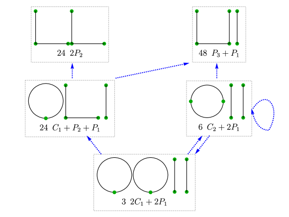
Figure 1. Multigraphs (unlabelled) given by the degree sequence $(2,2,1,1,1,1)$ in Example 3.5.

Example 3.6.

As another example, let $n=7$ and $\mathbf{d}=(2,2,2,1,1,1,1)$; thus there are $N/2=5$ edges. Suppose that a realization of the configuration model yields the multigraph $\mathsf{C}_{1}+\mathsf{C}_{2}+2\mathsf{P}_{1}$ in Figure 2. There are three bad edges: one loop and two parallel edges.

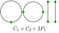
Figure 2. A multigraph given by the degree sequence $(2,2,2,1,1,1,1)$ in Example 3.6.

If we choose to first switch the loop, then with probability $\frac{1}{2}$ we switch it with one of the parallel edges, yielding the simple graph $\mathsf{C}_{3}+2\mathsf{P}_{1}$. If instead we switch the loop with one of the isolated edges, the result is $\mathsf{C}_{2}+\mathsf{P}_{2}+\mathsf{P}_{1}$, which after a second switching yields either a simple graph $\mathsf{P}_{4}+\mathsf{P}_{1}$ or $\mathsf{P}_{3}+\mathsf{P}_{2}$, or (if we switch the two parallel edges with each other) $\mathsf{C}_{2}+\mathsf{P}_{2}+\mathsf{P}_{1}$ again or $2\mathsf{C}_{1}+\mathsf{P}_{2}+\mathsf{P}_{1}$; in the latter cases, we obtain $\mathsf{P}_{4}+\mathsf{P}_{1}$ or $\mathsf{P}_{3}+\mathsf{P}_{2}$ after further switchings. Hence, the probability that the final graph contains a cycle $\mathsf{C}_{3}$ is $\frac{1}{2}$.

On the other hand, if we begin by switching one of the parallel edges, then there are three possibilities:

1. With probability $\frac{1}{4}$, we switch with the loop, and obtain again $\mathsf{C}_{3}+2\mathsf{P}_{1}$.

2. With probability $\frac{1}{2}$ we switch with an isolated edge and obtain $\mathsf{C}_{1}+\mathsf{P}_{3}+\mathsf{P}_{1}$ and after a second switching either $\mathsf{P}_{4}+\mathsf{P}_{1}$ or $\mathsf{P}_{3}+\mathsf{P}_{2}$.

3. With probability $\frac{1}{4}$ we switch the two parallel edges with each other, yielding either (with probability $\frac{1}{8}$ each) the same multigraph $\mathsf{C}_{1}+\mathsf{C}_{2}+2\mathsf{P}_{1}$ and we restart, or $3\mathsf{C}_{1}+2\mathsf{P}_{1}$. In the latter case, we next switch a loop with either (probability $\frac{1}{2}$ each) another loop, yielding $\mathsf{C}_{1}+\mathsf{C}_{2}+2\mathsf{P}_{1}$ and we restart, or with an isolated edge, yielding $2\mathsf{C}_{1}+\mathsf{P}_{2}+\mathsf{P}_{1}$, which eventually yields either $\mathsf{P}_{4}+\mathsf{P}_{1}$ or $\mathsf{P}_{3}+\mathsf{P}_{2}$.

Summing up this case, we start again with a graph $\mathsf{C}_{1}+\mathsf{C}_{2}+2\mathsf{P}_{1}$ with probability $\frac{3}{16}$, and thus the total probability that we end with case (i) is $\frac{1}{4}/\frac{13}{16}=\frac{4}{13}$.

Consequently, conditioned on this realisation of $G^{*}(7,\mathbf{d})$, the probability that the final graph $\widehat{G}(7,\mathbf{d})$ has a cycle $\mathsf{C}_{3}$ is $\frac{1}{2}$ or $\frac{4}{13}$, depending on our choice for the first switching. This shows that the order of the switchings matters. However, Theorem 2.1 is valid in any case, and thus such choices make no difference asymptotically.

With the modification in Remark 3.3, we never switch two parallel edges with each other so some possibilities disappear in this example; the final probabilities are $\frac{1}{2}$ and $\frac{1}{3}$, but the conclusion remains the same.

Example 3.7.

Fix $a>0$, consider for simplicity only even $n$, and let $\mathbf{d}:=(m,m,1,\dots,1)$, where $m:=\lfloor\sqrt{an}\rfloor$. Thus all vertices except 1 and 2 have degree 1. Note that (1.1) holds, but not (2.7).

Let $L_{1}$ and $L_{2}$ be the numbers of loops at 1 and 2, and let $M_{12}$ be the number of edges 12 in the multigraph $G^{*}(n,\mathbf{d})$. Note that besides these edges, $G(n,\mathbf{d})$ contains $m-2L_{j}-M_{12}$ edges from $j$ to a leaf ($j=1,2$), and a perfect matching of all remaining vertices. In particular, there are $n/2-O(n^{1/2})$ isolated edges.

The multigraph $G^{*}(n,\mathbf{d})$ is simple if $L_{1}=L_{2}=0$ and $M_{12}\leqslant 1$. It is easy to see, e.g. by the method of moments, that asymptotically, $L_{1}\overset{\mathrm{d}}{\longrightarrow}\operatorname{Po}(a/2)$, $L_{2}\overset{\mathrm{d}}{\longrightarrow}\operatorname{Po}(a/2)$, and $M_{12}\overset{\mathrm{d}}{\longrightarrow}\operatorname{Po}(a)$, jointly with independent limits. When we construct $\widehat{G}(n,\mathbf{d})$ by switchings, there is thus only $O_{\mathrm{p}}(1)$ bad edges; moreover, w.h.p. each switching will be with one of the $n/2-O(n^{1/2})$ isolated edges. In this case, no new bad edge is created by the switchings, and we reach a simple graph $\widehat{G}(n,\mathbf{d})$ after $L_{1}+L_{2}+(M_{12}-1)_{+}$ switchings; furthermore, no edge 12 is created by the switchings. It follows that w.h.p. $\widehat{G}(n,\mathbf{d})$ has an edge $12$ if and only if $M_{12}\geqslant 1$. Consequently,

$$\operatorname{\mathbb{P}{}}\bigl{(}12\in E(\widehat{G}(n,\mathbf{d}))\bigr{)}=\operatorname{\mathbb{P}{}}(M_{12}\geqslant 1)+o(1)\to\operatorname{\mathbb{P}{}}\bigl{(}\operatorname{Po}(a)\geqslant 1\bigr{)}=1-e^{-a}.$$ (3.3)

On the other hand, a simple graph with degree sequence $\mathbf{d}$ has either

1. no edge 12 and $m$ edges from each of 1 and 2 to leaves $k\geqslant 3$, together with a perfect matching of the remaining $n-2m-2$ vertices.

2. an edge 12 and $m-1$ edges from each of 1 and 2 to leaves $k\geqslant 3$, together with a perfect matching of the remaining $n-2m$ vertices.

Let the numbers of graphs of these two types be $N_{0}$ and $N_{1}$. Then

$$N_{0} =\binom{n-2}{m}\binom{n-2-m}{m}(n-2m-3)!!$$ (3.4)

$$N_{1} =\binom{n-2}{m-1}\binom{n-1-m}{m-1}(n-2m-1)!!$$ (3.5)

and a simple calculation yields

$$\frac{N_{1}}{N_{0}}=\frac{m^{2}}{n-2m}\to a.$$ (3.6)

Hence,

$$\operatorname{\mathbb{P}{}}\bigl{(}12\in E(G(n,\mathbf{d}))\bigr{)}=\frac{N_{1}}{N_{0}+N_{1}}\to\frac{a}{1+a}.$$ (3.7)

Comparing (3.3) and (3.7), we see that the limits differ, and thus Theorem 2.1 does not hold for this example. Similarly, Corollaries 2.2 and 2.3 fail, for example if $f_{n}(G)$ is the indicator of the event that the multigraph $G$ contains an edge where both endpoints have degrees $\geqslant 2$. This example shows that the condition (2.7) cannot be omitted from Theorem 2.1 and its corollaries.

Example 3.8.

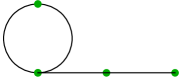
Figure 3. A multigraph given by the degree sequence $(3,2,1,1)$ in Example 3.8.

Let $\mathbf{d}=(3,2,2,1)$, and suppose that the initial multigraph $G^{*}(4,\mathbf{d})$ has edges 12, 12, 13, 34, see Figure 3. If we switch one of the parallel edges 12 with 34, then we may get a simple graph, but we may also create another edge 13 and get the edge set 12, 13, 13, 24. The latter multigraph is isomorphic to the original one, and we may continue and cycle between these two multigraphs for ever. Hence, there is no deterministic guarantee that the switching process always leads to a simple graph. Note also the modification in Remark 3.3 does not help; we still can make the same switchings.

However, note that in this example, switching the same edges but in different orientations yields a simple graph. Since we order the half-edges at random when switching, the infinite sequence of switchings above has probability 0; more generally, it is easily verified that for this example, a.s. the process terminates after a finite number of switchings.

4. The distribution of $\widehat{G}(n,\mathbf{d})$

4.1. More notation

Let $S$ be number of switchings used in the construction. Let $\Gamma_{k}$ ($0\leqslant k\leqslant S$) be the configuration after $k$ switchings, and let $G_{k}$ be the corresponding multigraph. Thus $G^{*}(n,\mathbf{d})=G_{0}$ and $\widehat{G}(n,\mathbf{d})=G_{S}$.

Let $\mathcal{B}_{k}$ be the set of endpoints of bad edges in $G_{k}$, and let $\mathcal{A}_{k}$ be the set of their neighbours in $G_{k}$.

Let $b_{k}$ be the bad edge in $\Gamma_{k-1}$ chosen for the $k$th switching, and let $e_{k}$ be the (random) other edge used in that switching.

An $m$-edge (in a graph or configuration) is a set of $m$ parallel edges that are not loops, and such that there are no further edges parallel to them. (I.e., the multiplicity of the edge equals $m$.) Let $L$ be the number of loops in $\Gamma_{0}$ (i.e., in $G_{0}=G^{*}(n,\mathbf{d})$), and let $M_{m}$ ($m\geqslant 2$) be the number of $m$-edges. Furthermore, let

$$M:=\sum_{m\geqslant 2}\binom{m}{2}M_{m},$$ (4.1)

the number of pairs of parallel edges in $\Gamma_{0}$.

Let ${\mathfrak{G}}_{n}$ be the set of all simple graphs on $[n]$ with degree sequence $\mathbf{d}$. Let $\lambda\in\mathcal{P}({\mathfrak{G}}_{n})$ be the distribution of $G(n,\mathbf{d})$, i.e., the uniform distribution on ${\mathfrak{G}}_{n}$, and let $\widehat{\lambda}\in\mathcal{P}({\mathfrak{G}}_{n})$ be the distribution of $\widehat{G}(n,\mathbf{d})$.

We sometimes tacitly assume that $n$ (and thus $N$) is large enough to avoid trivialities (such as division by 0).

4.2. Silver and golden

We say that the construction of $\widehat{G}(n,\mathbf{d})$ is silver if

1. No new bad edge is created during the construction.

2. No additional edge $e_{k}$ used for a switching has an endpoint in $\mathcal{B}_{0}$.

The construction is golden if it is silver and furthermore

1. $G^{*}(n,\mathbf{d})$ has no triple edges. I.e., $M_{m}=0$ for $m\geqslant 3$.

2. The loops and double edges in $G^{*}(n,\mathbf{d})$ are vertex-disjoint.

3. The additional edges $e_{k}$ used for the switchings are vertex-disjoint with each other.

Let ${\mathcal{S}}$ and $\mathcal{G}$ be the events that the construction is silver or golden, respectively, and let ${\mathcal{S}}^{\textsf{c}}$ and $\mathcal{G}^{\textsf{c}}$ be their complements. Furthermore, let ${\mathcal{S}}_{s}:={\mathcal{S}}\cap\{S=s\}$ and $\mathcal{G}_{s}:=\mathcal{G}\cap\{S=s\}$ ($s\geqslant 0$).

In a silver construction, each $m$-edge is reduced to a single (good) edge by $m-1$ switchings, and thus

$$S=L+\sum_{m\geqslant 2}(m-1)M_{m}.$$ (4.2)

In particular, in a golden construction, recalling (4.1),

$$S=L+M_{2}=L+M.$$ (4.3)

In a silver construction, (4.2) and (4.1) yield the inequality

$$S\leqslant L+M.$$ (4.4)

Lemma 4.1.

(i)  If (1.1) holds, then the construction of $\widehat{G}(n,\mathbf{d})$ is w.h.p. silver.

(ii)  If (1.1) and (2.7) hold, then the construction of $\widehat{G}(n,\mathbf{d})$ is w.h.p. golden.

Proof.

4.1: A well-known simple calculation shows that, assuming (1.1),

$$\operatorname{\mathbb{E}{}}L =\sum_{i}\frac{d_{i}(d_{i}-1)}{2(N-1)}\leqslant\frac{1}{N}\sum_{i=1}^{n}d_{i}(d_{i}-1)\leqslant\frac{1}{N}\sum_{i=1}^{n}d_{i}^{2}=O(1),$$ (4.5)

$$\operatorname{\mathbb{E}{}}M =\sum_{i<j}\frac{d_{i}(d_{i}-1)d_{j}(d_{j}-1)}{2(N-1)(N-3)}\leqslant C\biggl{(}\frac{1}{N}\sum_{i=1}^{n}d_{i}(d_{i}-1)\biggr{)}^{2}=O(1).$$ (4.6)

Hence, $\operatorname{\mathbb{E}{}}(L+M)=O(1)$, i.e., there is a constant $C$ such that

$$\operatorname{\mathbb{E}{}}(L+M)\leqslant C.$$ (4.7)

Fix a large integer $K$, and assume that $L+M\leqslant K$. Then $|\mathcal{B}_{0}|\leqslant L+2M\leqslant 2K$. Let $k\geqslant 0$, and suppose that the construction has been silver for the first $k$ switchings (in the obvious sense). Thus no new bad edges have been created and hence $\mathcal{B}_{k}\subseteq\mathcal{B}_{0}$. By the Cauchy–Schwarz inequality and (1.1), the number of half-edges belonging to vertices in $\mathcal{B}_{0}$ is

$$\sum_{i\in\mathcal{B}_{0}}d_{i}\leqslant\Bigl{(}|\mathcal{B}_{0}|\sum_{i\in\mathcal{B}_{0}}d_{i}^{2}\Bigr{)}^{1/2}\leqslant(2K)^{1/2}\Bigl{(}\sum_{i=1}^{n}d_{i}^{2}\Bigr{)}^{1/2}=O\bigl{(}n^{1/2}\bigr{)},$$ (4.8)

and thus

$$|\mathcal{A}_{k}|\leqslant\sum_{i\in\mathcal{B}_{k}}d_{i}\leqslant\sum_{i\in\mathcal{B}_{0}}d_{i}=O\bigl{(}n^{1/2}\bigr{)}.$$ (4.9)

Furthermore, the number of half-edges belonging to vertices in $\mathcal{A}_{k}$ is, by the argument in (4.8) together with (4.9),

$$\sum_{i\in\mathcal{A}_{k}}d_{i}\leqslant\Bigl{(}|\mathcal{A}_{k}|\sum_{i=1}^{n}d_{i}^{2}\Bigr{)}^{1/2}=O\bigl{(}|\mathcal{A}_{k}|^{1/2}n^{1/2}\bigr{)}=O\bigl{(}n^{3/4}\bigr{)}.$$ (4.10)

It follows from (4.8) and (4.10) that when we pick a random edge $e_{k+1}$ for the next switching, the probability that it has an endpoint in $\mathcal{B}_{0}$ or $\mathcal{A}_{k}$ is $O(n^{-1/4})=o(1)$. Hence, w.h.p. we switch with an edge $e_{k+1}$ not having any endpoint in $\mathcal{B}_{k}\cup\mathcal{A}_{k}$, and it is easy to see that then no new bad edge is created. Furthermore, w.h.p. $e_{k+1}$ has no endpoint in $\mathcal{B}_{0}$. Consequently, w.h.p. the construction remains silver for the $(k+1)$th swithching too. Since only $L+M\leqslant K$ switchings are needed, it follows by induction that w.h.p. the construction is silver until the end.

We have shown that for every fixed $K$, $\operatorname{\mathbb{P}{}}\bigl{(}{\mathcal{S}}^{\textsf{c}}\cap\{L+M\leqslant K\}\bigr{)}\to 0$. Hence, using also Markov’s inequality and (4.7),

$$\operatorname{\mathbb{P}{}}({\mathcal{S}}^{\textsf{c}}) \leqslant\operatorname{\mathbb{P}{}}\bigl{(}{\mathcal{S}}^{\textsf{c}}\cap\{L+M\leqslant K\}\bigr{)}+\operatorname{\mathbb{P}{}}\bigl{(}L+M>K\bigr{)}\leqslant o(1)+\frac{\operatorname{\mathbb{E}{}}(L+M)}{K}$$

$$\leqslant o(1)+\frac{C}{K}.$$ (4.11)

Thus $\limsup_{n\to\infty}\operatorname{\mathbb{P}{}}({\mathcal{S}}^{\textsf{c}})\leqslant C/K$. Since $K$ is arbitrary, $\operatorname{\mathbb{P}{}}({\mathcal{S}}^{\textsf{c}})\to 0$.

4.1: The expected number of triples of parallel edges in $G^{*}(n,\mathbf{d})$ is at most, using (1.1) and (2.7),

$$\sum_{i<j}d_{i}^{3}d_{j}^{3}\frac{C}{N^{3}}\leqslant C\frac{d_{\text{\rm max}}^{2}}{N^{3}}\Bigl{(}\sum_{i}d_{i}^{2}\Bigr{)}^{2}\leqslant C\frac{d_{\text{\rm max}}^{2}}{n}=o(1).$$ (4.12)

Hence, (G1) holds w.h.p.

Similar calculations show that the expected number of pairs of 2 loops, a loop and a double edge, or 2 double edges, are $o(1)$. Hence, (G2) holds w.h.p.

Finally, fix $k\geqslant 1$. Given $e_{1},\dots,e_{k-1}$, these have (at most) $2(k-1)$ endpoints. There are at most $2(k-1)d_{\text{\rm max}}$ edges with an endpoint in this set. Since $e_{k}$ is drawn at random among the $N/2-1$ edges distinct from $b_{k}$, the probability that $e_{k}$ is not vertex-disjoint from $e_{1},\dots,e_{k-1}$ is at most $2(k-1)d_{\text{\rm max}}/(N/2-1)=o(1)$. Note also that if the construction is silver and $L+M\leqslant K$, then at most $K$ switchings are done by (4.4). It follows that for any fixed $K$,

$$\operatorname{\mathbb{P}{}}\bigl{(}\mathcal{G}^{\textsf{c}}\cap{\mathcal{S}}\cap\{L+M\leqslant K\}\bigr{)}=o(1).$$ (4.13)

The argument in (and after) (4.2) shows that $\operatorname{\mathbb{P}{}}\bigl{(}\mathcal{G}^{\textsf{c}}\cap{\mathcal{S}}\bigr{)}\to 0$. Hence, using also part 4.1, $\operatorname{\mathbb{P}{}}\bigl{(}\mathcal{G}^{\textsf{c}}\bigr{)}\leqslant\operatorname{\mathbb{P}{}}\bigl{(}\mathcal{G}^{\textsf{c}}\cap{\mathcal{S}}\bigr{)}+\operatorname{\mathbb{P}{}}\bigl{(}{\mathcal{S}}^{\textsf{c}}\bigr{)}\to 0$. ∎

Proof of Theorem 3.2.

Immediate from Lemma 4.14.1, since a silver construction creates no new bad edges by (S1) and uses $S\leqslant L+M$ switchings by (4.4), so $\operatorname{\mathbb{E}{}}S\leqslant\operatorname{\mathbb{E}{}}(L+M)=O(1)$ by (4.7) and thus $S=O_{\mathrm{p}}(1)$. ∎

4.3. The choice of a bad edge

As said in Remark 3.1, the random graph $\widehat{G}(n,\mathbf{d})$ may depend on the (unspecified) rule for choosing the bad edge for each switching. However, all rules yield asymptotically the same result, at least provided (1.1) holds.

Lemma 4.2.

Assume (1.1). Let $\widehat{G}_{1}(n,\mathbf{d})$ and $\widehat{G}_{2}(n,\mathbf{d})$ be created by using two different rules for choosing the bad edge for each switching. Then $d_{\mathrm{TV}}(\widehat{G}_{1}(n,\mathbf{d}),\widehat{G}_{2}(n,\mathbf{d}))\to 0$.

Proof.

Suppose that we have a silver construction of $\widehat{G}_{1}(n,\mathbf{d})$; then only edges that are bad already in $\Gamma_{0}$ will be switched. It follows that we may couple the two constructions of $\widehat{G}(n,\mathbf{d})$, starting with the same $\Gamma_{0}$, such that if the construction of $\widehat{G}_{1}(n,\mathbf{d})$ is silver, then, in the sequence of graphs $G_{0},\dots,G_{S}=\widehat{G}(n,\mathbf{d})$, exactly the same switchings are made in both constructions, although perhaps in different order; consequently, the two constructions yield the same $\widehat{G}(n,\mathbf{d})$. (On the level of configurations, the switchings may differ, because of the choice of one parallel edge out of several.) Consequently, for this coupling, by Lemma 4.14.1,

$$\operatorname{\mathbb{P}{}}\bigl{(}\widehat{G}_{1}(n,\mathbf{d})\neq\widehat{G}_{2}(n,\mathbf{d})\bigr{)}=o(1).$$ (4.14)

This proves the lemma by (2.5). ∎

Lemma 4.2 implies that if Theorem 2.1 or Theorem 2.4 holds for some rule, then it holds for any rule. We may thus for the proofs below assume that we each time choose the bad edge in $\Gamma_{k}$ that is first according to the following order.

1. First the loops, in lexicographic order.

2. The $m$-edges in lexicographic order of their endpoints, and for each $m$-edge its $m$ edges in $\Gamma_{k}$ in lexicographic order.

The exact definition of the lexicographic order in these cases is left to the reader. In fact, any fixed order would do.

4.4. The subsubsequence principle

Next we note that it suffices to prove that Theorems 2.1 and 2.4 always hold for some subsequence. This is a general argument, which we repeat for convenience: Suppose that Theorem 2.1 fails; then there exists a sequence $\mathbf{d}_{n}$ satisfying the assumptions and such that (2.8) fails; thus there exists $\varepsilon>0$ and a subsequence such that $d_{\mathrm{TV}}\bigl{(}\widehat{G}(n,\mathbf{d}),G(n,\mathbf{d})\bigr{)}\geqslant\varepsilon$ for every $n$ in the subsequence. But by assumption we can find a subsubsequence such that Theorem 2.1 holds, a contradiction. The proof for Theorem 2.4 is essentially the same.

In particular, assuming (1.1), by selecting a suitable subsequence we may in the remainder of the proofs assume that (1.2) holds for some $\mu>0$ and $\mu_{2}<\infty$. Let $\nu:=\mu_{2}-\mu$; then (1.2) implies $N/n\to\mu$ and

$$\frac{1}{n}\sum_{i=1}^{n}d_{i}(d_{i}-1)\to\nu, \frac{1}{N}\sum_{i=1}^{n}d_{i}(d_{i}-1)\to\frac{\nu}{\mu}.$$ (4.15)

If $\nu=0$, then (4.15) and (4.5)–(4.6) show that $\operatorname{\mathbb{E}{}}L\to 0$ and $\operatorname{\mathbb{E}{}}M\to 0$. Consequently, w.h.p. $L=M=0$, so $G^{*}(n,\mathbf{d})$ is simple, in which case $\widehat{G}(n,\mathbf{d})=G^{*}(n,\mathbf{d})$; thus $d_{\mathrm{TV}}(\widehat{G}(n,\mathbf{d}),G^{*}(n,\mathbf{d}))\to 0$. Furthermore, by the fact that $G(n,\mathbf{d})$ has the same distribution as $G^{*}(n,\mathbf{d})$ conditioned on being simple, we can couple $G(n,\mathbf{d})$ and $G^{*}(n,\mathbf{d})$ such that they are equal when $G^{*}(n,\mathbf{d})$ is simple; thus by (2.5),

$$d_{\mathrm{TV}}(G(n,\mathbf{d}),G^{*}(n,\mathbf{d}))\leqslant\operatorname{\mathbb{P}{}}\bigl{(}G^{*}(n,\mathbf{d})\text{ is not simple}\bigr{)}\to 0.$$ (4.16)

Hence Theorems 2.1 and 2.4 follow trivially when $\nu=0$. Consequently, in the proofs we may assume $\nu>0$.

4.5. Silver constructions

Consider a silver construction. Each switching of a loop creates a copy of $\mathsf{P}_{2}$, and each set of $m-1$ switchings of an $m$-edge creates $m-1$ copies of $\mathsf{P}_{3}$ having a common middle edge, which is the one edge remaining of the original $m$ parallel ones. Colour the created copies of $\mathsf{P}_{2}$ and $\mathsf{P}_{3}$ red; these are regarded as (not necessarily disjoint) subgraphs of the configuration. Note that the non-leaves in the red paths belong to $\mathcal{B}_{0}$, while a leaf is an endpoint of some $e_{k}$ and thus, by (S2), lies outside $\mathcal{B}_{0}$. By (S2), the edges in the red paths will not be used by later switchings, and thus the red paths remain as subgraphs of $\Gamma_{S}$, and thus of $G_{S}=\widehat{G}(n,\mathbf{d})$.

The red paths do not have to be vertex-disjoint. However, by the remarks above and (S1)–(S2), the set ${\mathcal{R}}$ of red paths in $\Gamma_{S}$, or equivalently in $G_{S}=\widehat{G}(n,\mathbf{d})$, has the following properties.

1. Each red path has length 2 or 3, i.e., is a copy of $\mathsf{P}_{2}$ or $\mathsf{P}_{3}$.

2. The red paths are edge-disjoint, except that several red paths $\mathsf{P}_{3}$ may share the same middle edge.

3. An leaf of a red path is not a non-leaf of another red path.

Define the gap of a red path as its pair of endpoints. This is the pair of endpoints of the edge $e_{k}$ used to create this red path. By (S1) and (S2), $e_{k}$ was a good edge in $\Gamma_{0}$, i.e., there was no parallel edge in $\Gamma_{0}$. Thus the red paths have also the properties:

1. The gaps of the red paths are distinct pairs of vertices.

2. The gaps of the red paths are non-edges in $G_{S}$.

Furthermore, by (B2):

1. If a red $\mathsf{P}_{3}$ is given by the edges $i_{\alpha}j_{\beta}$, $j_{\gamma}k_{\delta}$, $k_{\varepsilon}\ell_{\zeta}$ in $\Gamma_{S}$, then necessarily the edge $j_{\gamma}k_{\delta}$ comes after $j_{\beta}k_{\varepsilon}$ in the lexicographic order.

Conversely, in a silver construction, the red paths in $\Gamma_{S}$ determine precisely the switchings that have been made; hence they together with $\Gamma_{S}$ determine the initial configuration $\Gamma_{0}$ and also, by (B1)–(B2), the order of the switchings. Moreover, given any simple configuration $\Gamma$ (on the given set of half-edges) with corresponding graph $G$ and a set of red paths in $\Gamma$ (or $G$) satisfying (P1)–(P6) (with obvious notational changes here and below: $\Gamma_{S}$ is replaced by $\Gamma$ and $G_{S}$ by $G$), there exists a unique initial configuration $\Gamma_{0}$ and a unique silver sequence of switchings, satisfying (B1)–(B2), that yields $\Gamma_{S}=\Gamma$ with the given red paths. Each such history with a given number $S$ of switchings has the same probability.

Consequently, dropping “red”:

Claim 1.

For a fixed $s\geqslant 0$, the conditional probability $\operatorname{\mathbb{P}{}}\bigl{(}\Gamma_{S}=\Gamma\mid{\mathcal{S}}_{s}\bigr{)}$ is proportional to the number of sets of $s$ paths in $\Gamma$ that satisfy (P1)–(P6).

We project to graphs. For a simple graph $G$ and a configuration $\Gamma$ projecting to $G$, there is an obvious bijection between sets of paths in $G$ and sets of paths in $\Gamma$. Note that the conditions (P1)–(P5) depend only on the paths in $G$, while (P6) depends also on the specific configuration $\Gamma$.

Given a simple graph $G\in{\mathfrak{G}}_{n}$, and a set ${\mathcal{R}}$ of $s$ paths in $G$ that satisfy (P1)–(P5), let the weight $w({\mathcal{R}};G)$ be the probability that the lifting of ${\mathcal{R}}$ to paths in a configuration $\Gamma$, chosen uniformly at random among all configuration $\Gamma$ that project to $G$, satisfies also (P6). Furthermore, for $G\in{\mathfrak{G}}_{n}$ and $s\geqslant 0$, let $\zeta_{{\mathcal{S}},s}(G)$ be the sum of the weights of all sets of $s$ paths in $G$ that satisfy (P1)–(P5).

Recall that each simple graph $G\in{\mathfrak{G}}_{n}$ is the projection of the same number $A:=\prod_{i}d_{i}!$ of configurations. It follows that the number of pairs $(\Gamma,{\mathcal{R}})$ where $\Gamma$ is a configuration projecting to $G$ and ${\mathcal{R}}$ is a set of $s$ paths in $\Gamma$ satisfying (P1)–(P6) equals $\sum_{{\mathcal{R}}}w({\mathcal{R}};G)A=A\zeta_{{\mathcal{S}},s}(G)$. Consequently, Claim 1 implies:

Claim 2.

For a fixed $s\geqslant 0$, and all $G\in{\mathfrak{G}}_{n}$, the conditional probability $\operatorname{\mathbb{P}{}}\bigl{(}\widehat{G}(n,\mathbf{d})=G\mid{\mathcal{S}}_{s}\bigr{)}$ is proportional to $\zeta_{{\mathcal{S}},s}(G)$.

Let $\widehat{\lambda}_{{\mathcal{S}},s}$ be the distribution of $\widehat{G}(n,\mathbf{d})$ conditioned on ${\mathcal{S}}_{s}$, i.e.,

$$\widehat{\lambda}_{{\mathcal{S}},s}\{G\}=\operatorname{\mathbb{P}{}}\bigl{(}\widehat{G}(n,\mathbf{d})=G\mid{\mathcal{S}}_{s}\bigr{)}.$$ (4.17)

Claim 2 says that the probability $\widehat{\lambda}_{{\mathcal{S}},s}(G)$ is proportional to $\zeta_{{\mathcal{S}},s}(G)$, and thus to $\zeta_{{\mathcal{S}},s}(G)\lambda\{G\}$, recalling that $\lambda$ is the uniform distribution. To find the normalizing constant, recall that $\lambda$ is the distribution of $G(n,\mathbf{d})$, which implies, using the notation $Z_{{\mathcal{S}},s}:=\zeta_{{\mathcal{S}},s}\bigl{(}G(n,\mathbf{d})\bigr{)}$,

$$\sum_{G\in{\mathfrak{G}}_{n}}\zeta_{{\mathcal{S}},s}(G)\lambda\{G\}=\operatorname{\mathbb{E}{}}\bigl{[}\zeta_{{\mathcal{S}},s}\bigl{(}G(n,\mathbf{d})\bigr{)}\bigr{]}=\operatorname{\mathbb{E}{}}Z_{{\mathcal{S}},s}.$$ (4.18)

Consequently, since $\widehat{\lambda}_{{\mathcal{S}},s}$ is a probability measure,

$$\widehat{\lambda}_{{\mathcal{S}},s}\{G\}=\frac{\zeta_{{\mathcal{S}},s}(G)}{\operatorname{\mathbb{E}{}}Z_{{\mathcal{S}},s}}\lambda\{G\}.$$ (4.19)

4.6. Golden constructions

For the proof of Theorem 2.1, we simplify and consider only golden constructions. In a golden construction, it follows from (G1)–(G3) that the red paths are vertex-disjoint. Conversely, a silver construction yielding vertex-disjoint red paths is golden.

It follows that Claims 1 and 2 above hold also if we replace ${\mathcal{S}}_{s}$ by $\mathcal{G}_{s}$ and consider only sets ${\mathcal{R}}$ of vertex-disjoint paths, so $\zeta_{{\mathcal{S}},s}(G)$ is replaced by $\zeta_{\mathcal{G},s}(G)$, defined as the total weight of all sets of $s$ vertex-disjoint paths in $G$ that satisfy (P1)–(P5). Thus, in analogy to (4.17)–(4.19), letting $\widehat{\lambda}_{\mathcal{G},s}$ be the distribution of $\widehat{G}(n,\mathbf{d})$ conditioned on $\mathcal{G}_{s}$, and $Z_{\mathcal{G},s}:=\zeta_{\mathcal{G},s}(G(n,\mathbf{d}))$,

$$\widehat{\lambda}_{\mathcal{G},s}\{G\}:=\operatorname{\mathbb{P}{}}\bigl{(}\widehat{G}(n,\mathbf{d})=G\mid\mathcal{G}_{s}\bigr{)}=\frac{\zeta_{\mathcal{G},s}(G)}{\operatorname{\mathbb{E}{}}Z_{\mathcal{G},s}}\lambda\{G\}.$$ (4.20)

Hence,

$$\lVert\widehat{\lambda}_{\mathcal{G},s}-\lambda\rVert_{\mathcal{M}({\mathfrak{G}}_{n})} =\sum_{G\in{\mathfrak{G}}_{n}}\bigl{\lvert}\widehat{\lambda}_{\mathcal{G},s}\{G\}-\lambda\{G\}\bigr{\rvert}=\sum_{G\in{\mathfrak{G}}_{n}}\Bigl{\lvert}\frac{{\zeta_{\mathcal{G},s}(G)-\operatorname{\mathbb{E}{}}Z_{\mathcal{G},s}}}{\operatorname{\mathbb{E}{}}Z_{\mathcal{G},s}}\Bigr{\rvert}\lambda\{G\}$$

$$=\frac{\operatorname{\mathbb{E}{}}\bigl{\lvert}Z_{\mathcal{G},s}-\operatorname{\mathbb{E}{}}Z_{\mathcal{G},s}\bigr{\rvert}}{\operatorname{\mathbb{E}{}}Z_{\mathcal{G},s}}.$$ (4.21)

This will be studied in the following sections. We first find the weights $w({\mathcal{R}};G)$.

Lemma 4.3.

Suppose that $G\in{\mathfrak{G}}_{n}$ and that ${\mathcal{R}}$ consists of $\ell\geqslant 0$ paths $\mathsf{P}_{2}$ and $m\geqslant 0$ paths $\mathsf{P}_{3}$ in $G$, all vertex-disjoint. Then the weight $w({\mathcal{R}};G)=2^{-m}$.

Proof.

Given any configuration projecting to $G$, we obtain all other such configurations by permuting the half-edges at each vertex. Hence, if $H\cong\mathsf{P}_{3}$ is a path in $G$, then it follows by symmetry, permuting only the half-edges at the two central vertices of $H$, that the probability is $\frac{1}{2}$ that (P6) holds for the lift of $H$ to a random configuration $\Gamma$ that projects to $G$. Furthermore, for disjoint $H_{1},\dots,H_{m}$, the corresponding events are independent. The result follows. ∎

For $\ell,m\geqslant 0$ and $G\in{\mathfrak{G}}_{n}$, let $\zeta_{\ell,m}(G)$ be the number of sets $\{F_{1},\dots,F_{\ell},\allowbreak H_{1},\dots,H_{m}\}$ of vertex-disjoint paths in $G$ such that each $F_{i}\cong\mathsf{P}_{2}$ and each $H_{j}\cong\mathsf{P}_{3}$, and (P5) holds. (We ignore the order of $F_{1},\dots,F_{\ell}$ and $H_{1},\dots,H_{m}$.) Note that (P2)–(P4) holds for any set of vertex-disjoint paths. Hence, Lemma 4.3 yields

$$\zeta_{\mathcal{G},s}(G)=\sum_{\ell+m=s}2^{-m}\zeta_{\ell,m}(G).$$ (4.22)

Remark 4.4.

The proof of Lemma 4.3 is easily extended to the more general sets of paths in Section 4.5. If the paths $\mathsf{P}_{3}$ in ${\mathcal{R}}$ are grouped according to their middle edges, with $m_{k}$ groups of $k-1$ paths having the same middle edge (and thus coming from switchings of an $k$-edge in $\Gamma_{0}$), $k\geqslant 2$, then $w({\mathcal{R}};G)=\prod_{k}k^{-m_{k}}$. We will not use this formula, and omit the details.

5. Some subgraph counts in $G^{*}(n,\mathbf{d})$

The equations (4.21) and (4.22) show that it suffices to show good estimates for the special subgraph counts $\zeta_{\ell,m}(G(n,\mathbf{d}))$. In order to do so, we use the standard method to study the random multigraph $G^{*}(n,\mathbf{d})$ instead (cf. Section 1). Let $Z^{*}_{\ell,m}:=\zeta_{\ell,m}\bigl{(}G^{*}(n,\mathbf{d})\bigr{)}$.

For two multigraphs $H$ and $G$, let $\psi_{H}(G)$ be the number of subgraphs of $G$ isomorphic to $H$. Define

$$X_{H}:=\psi_{H}\bigl{(}G^{*}(n,\mathbf{d})\bigr{)}.$$ (5.1)

Note that $L=X_{\mathsf{C}_{1}}$ and $M=X_{\mathsf{C}_{2}}$. We are mainly interested in the case when $H=\mathsf{P}_{2}$ or $\mathsf{P}_{3}$, and we write $X_{k}:=X_{\mathsf{P}_{k}}$.

We begin with an estimate that does not require (2.7).

Lemma 5.1.

Assume that $\mathbf{d}$ satisfies (1.1). Then, for every fixed $\ell,m\geqslant 0$,

$$\operatorname{\mathbb{E}{}}\bigl{(}X_{2}^{\ell}X_{3}^{m}\bigr{)}=O\bigl{(}n^{\ell+m}\bigr{)}.$$ (5.2)

Proof.

First, deterministically using (1.1), since there are at most $\binom{d_{i}}{2}$ copies of $\mathsf{P}_{2}$ with middle vertex $i$,

$$X_{2}\leqslant\sum_{i=1}^{n}\binom{d_{i}}{2}=O(n).$$ (5.3)

We estimate $X_{3}$ too from above by overcounting. For $i,j\in[n]$ and $\alpha\in[d_{i}]$, $\beta\in[d_{j}]$, let $I_{i,\alpha,j,\beta}$ be the indicator of the event that the half-edges $i_{\alpha}$ and $j_{\beta}$ form an edge. Then

$$X_{3}\leqslant\widehat{X}_{3}:=\sum_{i<j}\sum_{\alpha=1}^{d_{i}}\sum_{\beta=1}^{d_{j}}(d_{i}-1)(d_{j}-1)I_{i,\alpha,j,\beta}.$$ (5.4)

We show, by induction on $m$, that for every fixed $m\geqslant 0$,

$$\operatorname{\mathbb{E}{}}\widehat{X}_{3}^{m}=O\bigl{(}n^{m}\bigr{)}.$$ (5.5)

This is trivial for $m=0$, and for $m=1$ we have (cf. the similar (4.6))

$$\operatorname{\mathbb{E}{}}\widehat{X}_{3} =\sum_{i<j}\sum_{\alpha=1}^{d_{i}}\sum_{\beta=1}^{d_{j}}(d_{i}-1)(d_{j}-1)\operatorname{\mathbb{E}{}}I_{i,\alpha,j,\beta}=\sum_{i<j}\frac{d_{i}(d_{i}-1)d_{j}(d_{j}-1)}{N-1}$$

$$\leqslant\frac{C}{n}\left(\sum_{i=1}^{n}d_{i}(d_{i}-1)\right)^{2}=O(n).$$ (5.6)

For the induction step, note that (5.4) yields the expansion

$$\operatorname{\mathbb{E}{}}\widehat{X}_{3}^{m}=\sum_{i_{1}<j_{1},\dots,i_{m}<j_{m}}\sum_{\alpha_{1},\dots,\alpha_{m}}\sum_{\beta_{1},\dots,\beta_{m}}\operatorname{\mathbb{E}{}}\prod_{k=1}^{m}(d_{i_{k}}-1)(d_{j_{k}}-1)I_{i_{k},\alpha_{k},j_{k},\beta_{k}}.$$ (5.7)

First, let $1\leqslant k<\ell\leqslant m$, and consider all terms in (5.7) where $(i_{k},\alpha_{k},j_{k},\beta_{k})=(i_{\ell},\alpha_{\ell},j_{\ell},\beta_{\ell})$. In these terms, $I_{i_{\ell},\alpha_{\ell},j_{\ell},\beta_{\ell}}$ is redundant, and $(d_{i_{\ell}}-1)(d_{j_{\ell}}-1)<d_{\text{\rm max}}^{2}\leqslant Cn$, and eliminating these factors yields $\operatorname{\mathbb{E}{}}\widehat{X}_{3}^{m-1}$. Hence, the induction hypothesis shows that the contribution of these terms is at most $Cn\operatorname{\mathbb{E}{}}\widehat{X}_{3}^{m-1}=O(n^{m})$.

Summing over all pairs $(k,\ell)$ still yields $O(n^{m})$.

The remaining terms in (5.7) are those where the $m$ quadruples $(i_{k},\alpha_{k},j_{k},\beta_{k})$ are distinct. In this case, either

$$\operatorname{\mathbb{E}{}}\prod_{k=1}^{m}I_{i_{k},\alpha_{k},j_{k},\beta_{k}} =\frac{1}{(N-1)(N-3)\dotsm(N-2m+1)}$$ (5.8)

$$\leqslant\frac{C}{(N-1)^{m}}=C\prod_{k=1}^{m}\operatorname{\mathbb{E}{}}I_{i_{k},\alpha_{k},j_{k},\beta_{k}},$$ (5.9)

(where $C=C_{m}$ depends on $m$), or $\prod_{k=1}^{m}I_{i_{k},\alpha_{k},j_{k},\beta_{k}}=0$ identically because of conflicts. Consequently, the sum of these terms in (5.7) is at most

$$\sum_{i_{1}<j_{1},\dots,i_{m}<j_{m}}\sum_{\alpha_{1},\dots,\alpha_{m}}\sum_{\beta_{1},\dots,\beta_{m}}C\prod_{k=1}^{m}(d_{i_{k}}-1)(d_{j_{k}}-1)\operatorname{\mathbb{E}{}}I_{i_{k},\alpha_{k},j_{k},\beta_{k}}=C\bigl{(}\operatorname{\mathbb{E}{}}\widehat{X}_{3}\bigr{)}^{m}.$$ (5.10)

By (5), this too is $O(n^{m})$, which completes the induction step and proves (5.5). The result follows by (5.3) and (5.5). ∎

Lemma 5.2.

Assume that $\mathbf{d}$ satisfies (1.2) and (2.7). Then

$$\frac{X_{2}}{n} \overset{\mathrm{p}}{\longrightarrow}\frac{\nu}{2},$$ (5.11)

$$\frac{X_{3}}{n} \overset{\mathrm{p}}{\longrightarrow}\frac{\nu^{2}}{2\mu}.$$ (5.12)

Proof.

First, the overcount in (5.3) comes from the loops and multiple edges, and we have the estimate

$$0\leqslant\sum_{i=1}^{n}\binom{d_{i}}{2}-X_{2}\leqslant 2d_{\text{\rm max}}X_{\mathsf{C}_{1}}+2X_{\mathsf{C}_{2}}=2d_{\text{\rm max}}L+2M.$$ (5.13)

By (4.5)–(4.6), $L,M=O_{\mathrm{p}}(1)$, and thus (5.13) yields, using (2.7),

$$\frac{X_{2}}{n}=\frac{1}{n}\sum_{i=1}^{n}\binom{d_{i}}{2}+o_{\mathrm{p}}\bigl{(}n^{-1/2}\bigr{)}=\frac{1}{n}\sum_{i=1}^{n}\binom{d_{i}}{2}+o_{\mathrm{p}}(1).$$ (5.14)

Hence, (5.11) follows by (4.15).

For $X_{3}$, we consider again $\widehat{X}_{3}$ defined in (5.4). This too is defined by overcounting, and it is easily seen that

$$0\leqslant\widehat{X}_{3}-X_{3}\leqslant 2d_{\text{\rm max}}^{2}X_{\mathsf{C}_{1}}+4d_{\text{\rm max}}X_{\mathsf{C}_{2}}+3X_{\mathsf{C}_{3}}.$$ (5.15)

Again, $X_{\mathsf{C}_{1}}=L=O_{\mathrm{p}}(1)$ and $X_{\mathsf{C}_{2}}=M=O_{\mathrm{p}}(1)$ by (4.5)–(4.6), and a similar calculation shows $\operatorname{\mathbb{E}{}}X_{\mathsf{C}_{3}}=O(1)$ and thus $X_{\mathsf{C}_{3}}=O_{\mathrm{p}}(1)$. Furthermore, $d_{\text{\rm max}}=o(n^{1/2})$ by (2.7). Hence, (5.15) implies

$$\widehat{X}_{3}-X_{3}=o_{\mathrm{p}}(n).$$ (5.16)

Consequently, it suffices to consider $\widehat{X}_{3}$. We have, by (5),

$$\operatorname{\mathbb{E}{}}\widehat{X}_{3}=\frac{1}{2(N-1)}\left(\biggl{(}\sum_{i=1}^{n}d_{i}(d_{i}-1)\biggr{)}^{2}-\sum_{i=1}^{n}d_{i}^{2}(d_{i}-1)^{2}\right).$$ (5.17)

Furthermore, by (2.7) and (1.1),

$$\sum_{i=1}^{n}d_{i}^{2}(d_{i}-1)^{2}\leqslant d_{\text{\rm max}}^{2}\sum_{i=1}^{n}d_{i}^{2}=o(n^{2}).$$ (5.18)

Using (5.18) and (4.15) in (5.17) yields

$$\frac{\operatorname{\mathbb{E}{}}\widehat{X}_{3}}{n}\to\frac{\nu^{2}}{2\mu}.$$ (5.19)

Finally, we estimate the variance of $\widehat{X}_{3}$. We use again the representation (5.4). We have the covariances

$$\operatorname{Cov}\bigl{(}I_{i,\alpha,j,\beta},I_{k,\gamma,\ell,\delta}\bigr{)}=\begin{cases}\frac{1}{N-1}-\bigl{(}\frac{1}{N-1}\bigr{)}^{2},&\{i_{\alpha},j_{\beta}\}=\{k_{\gamma},\ell_{\delta}\},\\ -\bigl{(}\frac{1}{N-1}\bigr{)}^{2},&|\{i_{\alpha},j_{\beta}\}\cap\{k_{\gamma},\ell_{\delta}\}|=1,\\ \frac{1}{(N-1)(N-3)}-\bigl{(}\frac{1}{N-1}\bigr{)}^{2},&|\{i_{\alpha},j_{\beta}\}\cap\{k_{\gamma},\ell_{\delta}\}|=0.\end{cases}$$ (5.20)

Hence, whenever $\{i_{\alpha},j_{\beta}\}\neq\{k_{\gamma},\ell_{\delta}\}$,

$$\operatorname{Cov}\bigl{(}I_{i,\alpha,j,\beta},I_{k,\gamma,\ell,\delta}\bigr{)}\leqslant\frac{2}{(N-1)^{2}(N-3)}\leqslant\frac{C}{n}\operatorname{\mathbb{E}{}}I_{i,\alpha,j,\beta}\operatorname{\mathbb{E}{}}I_{k,\gamma,\ell,\delta},$$ (5.21)

and it follows from (5.4) that, using (5) and (2.7),

$$\operatorname{Var}\widehat{X}_{3} \leqslant\sum_{i<j}\sum_{\alpha=1}^{d_{i}}\sum_{\beta=1}^{d_{j}}(d_{i}-1)^{2}(d_{j}-1)^{2}\operatorname{\mathbb{E}{}}I_{i,\alpha,j,\beta}+\frac{C}{n}\bigl{(}\operatorname{\mathbb{E}{}}\widehat{X}_{3}\bigr{)}^{2}$$

$$\leqslant d_{\text{\rm max}}^{2}\operatorname{\mathbb{E}{}}\widehat{X}_{3}+\frac{C}{n}\bigl{(}\operatorname{\mathbb{E}{}}\widehat{X}_{3}\bigr{)}^{2}=O\bigl{(}nd_{\text{\rm max}}^{2}\bigr{)}+O\bigl{(}n\bigr{)}=o\bigl{(}n^{2}\bigr{)}.$$ (5.22)

Consequently, $(\widehat{X}_{3}-\operatorname{\mathbb{E}{}}\widehat{X}_{3})/n\overset{\mathrm{p}}{\longrightarrow}0$, which together with (5.19) implies

$$\frac{\widehat{X}_{3}}{n}\overset{\mathrm{p}}{\longrightarrow}\frac{\nu^{2}}{2\mu}.$$ (5.23)

Finally, this and (5.16) imply (5.12). ∎

Remark 5.3.

Lemma 5.2 may fail without the assumption (2.7). For an example, consider again Example 3.7. Then $\widehat{X}_{3}=(m-1)^{2}M_{12}$ and by an estimate similar to (5.15), $X_{3}=(m-1)^{2}M_{12}+o_{\mathrm{p}}(n)$; hence $X_{3}/n=aM_{12}+o_{\mathrm{p}}(1)\overset{\mathrm{d}}{\longrightarrow}a\operatorname{Po}(a)$. Thus $X_{3}/n$ does not converge in probability to a constant.

Remark 5.4.

Under the stronger assumption $\sum_{i}d_{i}^{m}=O(n)$ for every $m<\infty$, it is shown in [19, Theorem 3.10] that (for example) $X_{2}$ and $X_{3}$ are asymptotically normal, with variance of order $n$. We do not know whether that holds under the weaker assumptions in Lemma 5.2.

Lemma 5.5.

Assume that $\mathbf{d}$ satisfies (1.2) and (2.7). Then, for any $\ell,m\geqslant 0$,

$$n^{-\ell-m}Z^{*}_{\ell,m} \overset{\mathrm{p}}{\longrightarrow}\alpha_{\ell,m}:=\frac{1}{\ell!\,m!}\Bigl{(}\frac{\nu}{2}\Bigr{)}^{\ell}\Bigl{(}\frac{\nu^{2}}{2\mu}\Bigr{)}^{m}.$$ (5.24)

Proof.

$\ell!\,m!\,Z^{*}_{\ell,m}$ counts ordered sequences of subgraphs $F_{1},\dots,F_{\ell},\allowbreak H_{1},\dots,H_{m}$ of vertex-disjoint paths in $G^{*}(n,\mathbf{d})$ such that each $F_{i}\cong\mathsf{P}_{2}$ and each $H_{j}\cong\mathsf{P}_{3}$, and (P5) holds. We may overcount and estimate this by $X_{2}^{\ell}X_{3}^{m}$; we can also estimate the error by

$$0\leqslant X_{2}^{\ell}X_{3}^{m}-\ell!\,m!\,Z^{*}_{\ell,m}\\ \leqslant\binom{\ell}{2}A_{22}X_{2}^{\ell-2}X_{3}^{m}+\ell mA_{23}X_{2}^{\ell-1}X_{3}^{m-1}+\binom{m}{2}A_{33}X_{2}^{\ell}X_{3}^{m-2}\\ +\ell B_{2}X_{2}^{\ell-1}X_{3}^{m}+mB_{3}X_{2}^{\ell}X_{3}^{m-1},$$ (5.25)

where $A_{jk}$ is that number of pair of paths $F\cong\mathsf{P}_{j}$ and $F^{\prime}\cong\mathsf{P}_{k}$ in $G^{*}(n,\mathbf{d})$ such that $F\cap F^{\prime}\neq\emptyset$, and $B_{j}$ is the number of paths $\mathsf{P}_{j}$ such that (P5) does not hold, i.e. paths $\mathsf{P}_{j}$ that are part of a cycle $\mathsf{C}_{j+1}$.

We estimate $A_{jk}$ and $B_{j}$. First, we have $B_{2}\leqslant 3X_{\mathsf{C}_{3}}$ and $B_{3}\leqslant 4X_{\mathsf{C}_{4}}$. Calculations similar to (4.6) show $\operatorname{\mathbb{E}{}}X_{\mathsf{C}_{j}}=O(1)$ for any fixed $j$ (as said in the proof of Lemma 5.2 for $j=3$), and thus

$$B_{2} =O_{\mathrm{p}}(1), B_{3} =O_{\mathrm{p}}(1).$$ (5.26)

Fix $j,k\in\{2,3\}$. We make a decomposition

$$A_{jk}=\sum_{H\in\mathcal{H}}A_{jk}(H),$$ (5.27)

where $A_{jk}(H)$ is the number of pairs $(F,F^{\prime})$ of paths in $G^{*}(n,\mathbf{d})$ such that $F\cap F^{\prime}\neq\emptyset$, $F\cong\mathsf{P}_{j}$, $F^{\prime}\cong\mathsf{P}_{k}$ and $F\cup F^{\prime}\cong H$, and $\mathcal{H}$ is the (finite) set of unlabelled multigraphs that can be written as a union of two paths of lengths $j$ and $k$. Given $F\cup F^{\prime}$, there is $O(1)$ choices of $F$ and $F^{\prime}$, and thus

$$A_{ij}(H)\leqslant CX_{H}.$$ (5.28)

For $r\geqslant 0$, let

$$\Delta_{r}:=\sum_{i=1}^{n}d_{i}^{r}.$$ (5.29)

Let $H\in\mathcal{H}$ have $q$ vertices with degrees $\delta_{1},\dots,\delta_{q}$. Then the number of possible copies of $H$ in $G^{*}(n,\mathbf{d})$, counted in the corresponding configuration, is at most

$$\sum_{i_{1},\dots,i_{q}}\prod_{k=1}^{q}d_{i_{k}}^{\delta_{k}}=\prod_{k=1}^{q}\Delta_{\delta_{k}},$$ (5.30)

and each such copy occurs with probability $O(N^{-e(H)})=O(n^{-e(H)})$. Since $e(H)=\frac{1}{2}\sum_{k}\delta_{k}$,

$$\operatorname{\mathbb{E}{}}X_{H}\leqslant Cn^{-e(H)}\prod_{k=1}^{q}\Delta_{\delta_{k}}=C\prod_{k=1}^{q}n^{-\delta_{k}/2}\Delta_{\delta_{k}}.$$ (5.31)

By (1.1), $\Delta_{1}=O(n)$ and $\Delta_{2}=O(n)$. Furthermore, for $\delta>2$, $\Delta_{\delta}\leqslant d_{\text{\rm max}}^{\delta-2}\Delta_{2}\leqslant Cd_{\text{\rm max}}^{\delta-2}n$. Hence, using (2.7),

$$n^{-\delta/2}\Delta_{\delta}\leqslant\begin{cases}Cn^{1/2},&\delta=1,\\ C,&\delta=2,\\ Cd_{\text{\rm max}}^{\delta-2}n^{1-\delta/2}=o(1),&\delta>2.\end{cases}$$ (5.32)

Let $h_{1}$ be the number of vertices in $H$ with degree 1. Since $H$ is a connected union of two paths, $H$ has no isolated vertices, and it follows from (5.31) and (5.32) that $\operatorname{\mathbb{E}{}}X_{H}=O(n^{h_{1}/2})$. Furthermore, $h_{1}\leqslant 4$, and if $h_{1}=4$, then there is some vertex with degree $>2$. If $h_{1}\leqslant 3$, then $\operatorname{\mathbb{E}{}}X_{H}=O\bigl{(}n^{3/2}\bigr{)}$, and if $h_{1}=4$ and some vertex has degree $\delta>2$, then (5.31) and (5.32) imply $\operatorname{\mathbb{E}{}}X_{H}\leqslant Cn^{4/2}(d_{\text{\rm max}}/n^{1/2})^{\delta-2}=o\bigl{(}n^{2}\bigr{)}$.

Hence, $\operatorname{\mathbb{E}{}}X_{H}=o\bigl{(}n^{2}\bigr{)}$ for every $H\in\mathcal{H}$, and thus $\operatorname{\mathbb{E}{}}A_{jk}(H)=o\bigl{(}n^{2}\bigr{)}$ by (5.28), and finally $\operatorname{\mathbb{E}{}}A_{jk}=o\bigl{(}n^{2}\bigr{)}$ by (5.27), which implies

$$A_{jk}=o_{\mathrm{p}}\bigl{(}n^{2}\bigr{)}.$$ (5.33)

Since Lemma 5.2 implies $X_{2},X_{3}\leqslant Cn$ w.h.p., it follows from (5.26) that the last two terms in (5.25) are $O_{\mathrm{p}}\bigl{(}n^{\ell+m-1}\bigr{)}$, and from (5.33) that the remaining terms on the right-hand side are $o_{\mathrm{p}}\bigl{(}n^{\ell+m}\bigr{)}$. Consequently, (5.25) implies

$$X_{2}^{\ell}X_{3}^{m}-\ell!\,m!\,Z^{*}_{\ell,m}=o_{\mathrm{p}}\bigl{(}n^{\ell+m}\bigr{)}$$ (5.34)

and thus

$$n^{-\ell-m}Z^{*}_{\ell,m}=\frac{1}{\ell!\,m!}\left(\frac{X_{2}}{n}\right)^{\ell}\left(\frac{X_{3}}{n}\right)^{m}+o_{\mathrm{p}}(1)$$ (5.35)

and the result (5.24) follows from Lemma 5.2. ∎

Lemma 5.6.

Assume that $\mathbf{d}$ satisfies (1.2) and (2.7). Let $\ell,m\geqslant 0$. Then,

$$\operatorname{\mathbb{E}{}}|Z^{*}_{\ell,m}-\alpha_{\ell,m}n^{\ell+m}|=o\bigl{(}n^{\ell+m}\bigr{)}.$$ (5.36)

Proof.

Let $Y_{n}:=n^{-\ell-m}Z^{*}_{\ell,m}$. We have $Y_{n}\leqslant n^{-\ell-m}X_{2}^{\ell}X_{3}^{m}$ by (5.25), and thus by Lemma 5.1,

$$\operatorname{\mathbb{E}{}}[Y_{n}^{2}]\leqslant n^{-2\ell-2m}\operatorname{\mathbb{E}{}}\bigl{[}X_{2}^{2\ell}X_{3}^{2m}\bigr{]}=O(1).$$ (5.37)

Hence, the sequence $Y_{n}$ ($n\geqslant 1$) is uniformly integrable (see e.g. [13, Theorem 5.4.2]), and thus (5.24) implies $L^{1}$-convergence [13, Theorem 5.5.4], i.e.,

$$\operatorname{\mathbb{E}{}}\bigl{\lvert}Y_{n}-\alpha_{\ell,m}\bigr{\rvert}\to 0,$$ (5.38)

which is equivalent to (5.36). ∎

6. Proof of Theorem 2.1

We now transfer the results in Section 5 to the simple random graph $G(n,\mathbf{d})$.

Lemma 6.1.

The results in Lemmas 5.1, 5.2, 5.5, 5.6 hold also conditioned on the event that $G^{*}(n,\mathbf{d})$ is simple. In other words, the corresponding results for $G(n,\mathbf{d})$ hold as well.

Proof.

An immediate consequence of (1.3). ∎

Let $Z_{\ell,m}:=\zeta_{\ell,m}(G(n,\mathbf{d}))$.

Lemma 6.2.

Assume that $\mathbf{d}$ satisfies (1.2) and (2.7). Let $\ell,m\geqslant 0$. Then,

$$\operatorname{\mathbb{E}{}}Z_{\ell,m}=\bigl{(}\alpha_{\ell,m}+o(1)\bigr{)}n^{\ell+m},$$ (6.1)

$$\operatorname{\mathbb{E}{}}|Z_{\ell,m}-\operatorname{\mathbb{E}{}}Z_{\ell,m}|=o\bigl{(}n^{\ell+m}\bigr{)}.$$ (6.2)

Proof.

By Lemmas 5.6 and 6.1,

$$\operatorname{\mathbb{E}{}}\bigl{\lvert}Z_{\ell,m}-\alpha_{\ell,m}n^{\ell+m}\bigr{\rvert}=o\bigl{(}n^{\ell+m}\bigr{)}.$$ (6.3)

This implies (6.1), and then (6.1) and (6.3) yield (6.2). ∎

Proof of Theorem 2.1.

As said in Section 4.4, we may assume that (1.2) holds and $\nu>0$. Fix $s\geqslant 0$. Recalling the notations $Z_{\mathcal{G},s}:=\zeta_{\mathcal{G},s}\bigl{(}G(n,\mathbf{d})\bigr{)}$ and $Z_{\ell,m}:=\zeta_{\ell,m}\bigl{(}G(n,\mathbf{d})\bigr{)}$, we see that (4.22) and (6.2) imply that

$$\operatorname{\mathbb{E}{}}|Z_{\mathcal{G},s}-\operatorname{\mathbb{E}{}}Z_{\mathcal{G},s}|=o\bigl{(}n^{s}\bigr{)}.$$ (6.4)

Furthermore, (4.22) and (6.1) imply

$$\operatorname{\mathbb{E}{}}Z_{\mathcal{G},s}\geqslant\operatorname{\mathbb{E}{}}Z_{s,0}=\bigl{(}\alpha_{s,0}+o(1)\bigr{)}n^{s}.$$ (6.5)

Hence, using (4.21), noting that $\alpha_{s,0}>0$,

$$\lVert\widehat{\lambda}_{\mathcal{G},s}-\lambda\rVert_{\mathcal{M}({\mathfrak{G}}_{n})}=\frac{\operatorname{\mathbb{E}{}}|Z_{\mathcal{G},s}-\operatorname{\mathbb{E}{}}Z_{\mathcal{G},s}|}{\operatorname{\mathbb{E}{}}Z_{\mathcal{G},s}}\to 0.$$ (6.6)

Let $p_{s}:=\operatorname{\mathbb{P}{}}(\mathcal{G}_{s})$, and $p^{\textsf{c}}:=\operatorname{\mathbb{P}{}}(\mathcal{G}^{\textsf{c}})$. Then $p^{\textsf{c}}+\sum_{s}p_{s}=1$, and, recalling (4.20) and letting $\widehat{\lambda}_{\mathcal{G}}^{\textsf{c}}$ be the distribution of $\widehat{G}(n,\mathbf{d})$ conditioned on $\mathcal{G}^{\textsf{c}}$,

$$\widehat{\lambda}=p^{\textsf{c}}\widehat{\lambda}_{\mathcal{G}}^{\textsf{c}}+\sum_{s=0}^{\infty}p_{s}\widehat{\lambda}_{\mathcal{G},s}.$$ (6.7)

Consequently, for any $K\geqslant 1$, using (4.21),

$$\lVert\widehat{\lambda}-\lambda\rVert_{\mathcal{M}({\mathfrak{G}}_{n})} =\Bigl{\lVert}p^{\textsf{c}}(\widehat{\lambda}_{\mathcal{G}}^{\textsf{c}}-\lambda)+\sum_{s\geqslant 0}p_{s}(\widehat{\lambda}_{\mathcal{G},s}-\lambda)\Bigr{\rVert}_{\mathcal{M}({\mathfrak{G}}_{n})}$$

$$\leqslant p^{\textsf{c}}\lVert\widehat{\lambda}_{\mathcal{G}}^{\textsf{c}}-\lambda\rVert_{\mathcal{M}({\mathfrak{G}}_{n})}+\sum_{s\geqslant 0}p_{s}\lVert\widehat{\lambda}_{\mathcal{G},s}-\lambda\rVert_{\mathcal{M}({\mathfrak{G}}_{n})}$$

$$\leqslant 2p^{\textsf{c}}+\sum_{s=0}^{K}\lVert\widehat{\lambda}_{\mathcal{G},s}-\lambda\rVert_{\mathcal{M}({\mathfrak{G}}_{n})}+\sum_{s>K}2p_{s}.$$ (6.8)

By Lemma 4.14.1, $p^{\textsf{c}}=o(1)$, and by (6.6), $\lVert\widehat{\lambda}_{\mathcal{G},s}-\lambda\rVert_{\mathcal{M}({\mathfrak{G}}_{n})}=o(1)$ for every fixed $s$. Furthermore, recall that $\mathcal{G}_{s}$ implies $L+M=S=s$, see (4.3). Hence, for any fixed $K$, (6) implies, using (4.7),

$$\lVert\widehat{\lambda}-\lambda\rVert_{\mathcal{M}({\mathfrak{G}}_{n})} \leqslant o(1)+o(1)+\sum_{s>K}2\operatorname{\mathbb{P}{}}(L+M=s)=o(1)+2\operatorname{\mathbb{P}{}}(L+M>K)$$

$$\leqslant o(1)+\frac{2\operatorname{\mathbb{E}{}}(L+M)}{K}\leqslant o(1)+\frac{C}{K}.$$ (6.9)

Thus $\limsup_{n\to\infty}\lVert\widehat{\lambda}-\lambda\rVert_{\mathcal{M}({\mathfrak{G}}_{n})}\leqslant C/K$, and then letting $K\to\infty$ yields $\lVert\widehat{\lambda}-\lambda\rVert_{\mathcal{M}({\mathfrak{G}}_{n})}\to 0$. This completes the proof of (2.8) by (2.3). The final sentence follows by (2.5). ∎

Proof of Corollary 2.2.

Using a coupling such that (2.9) holds, we have $\operatorname{\mathbb{P}{}}(X_{n}\neq\widehat{X}_{n})\to 0$, and the conclusion follows. ∎

Proof of Corollary 2.3.

Let $\widehat{X}_{n}:=f_{n}\bigl{(}\widehat{G}(n,\mathbf{d})\bigr{)}$. Then the assumption (2.10) says $\widehat{X}_{n}-X^{*}_{n}\overset{\mathrm{p}}{\longrightarrow}0$. We have also assumed $X^{*}_{n}\overset{\mathrm{d}}{\longrightarrow}Y$, and it follows that $\widehat{X}\overset{\mathrm{d}}{\longrightarrow}Y$. Hence the result follows by Corollary 2.2. ∎

7. Proof of Theorem 2.4

Since we do not assume (2.7), the construction is not necessarily golden w.h.p. (There may be e.g. triple edges in $G^{*}(n,\mathbf{d})$.) Hence we use in this section silver constructions. Recall the notation $Z_{{\mathcal{S}},s}:=\zeta_{{\mathcal{S}},s}(G(n,\mathbf{d}))$.

We define, cf. (5.1), for a multigraph $H$,

$$Y_{H}:=\psi_{H}\bigl{(}G(n,\mathbf{d})\bigr{)}.$$ (7.1)

Lemma 7.1.

Assume that $\mathbf{d}$ satisfies (1.2) and $\nu>0$. Let $s\geqslant 0$. Then,

$$\operatorname{\mathbb{E}{}}Z_{{\mathcal{S}},s} \geqslant cn^{s},$$ (7.2)

$$\operatorname{\mathbb{E}{}}Z_{{\mathcal{S}},s}^{2} \leqslant Cn^{2s},$$ (7.3)

Proof.

(i): By selecting subsequences, see Section 4.4, we may assume that the limit $b:=\lim_{n\to\infty}d_{\text{\rm max}}/n^{1/2}$ exists. We consider two cases.

(ia): $b=0$. This means $d_{\text{\rm max}}=o(n^{1/2})$, i.e., (2.7) holds; thus Lemma 6.2 and its consequence (6.5) hold. By definition, $\zeta_{{\mathcal{S}},s}(G)\geqslant\zeta_{\mathcal{G},s}(G)$ for all $G\in{\mathfrak{G}}_{n}$. Hence, $Z_{{\mathcal{S}},s}\geqslant Z_{\mathcal{G},s}$, and (7.2) follows by (6.5).

(ib): $b>0$. We may assume that $d_{\text{\rm max}}=d_{1}$. Then, for large $n$, $d_{1}=d_{\text{\rm max}}\geqslant\frac{b}{2}n$. Say that a half-edge at vertex 1 is green if it is not part of a loop or multiple edge, and let $W$ be the number of green edges. Then $W\geqslant d_{1}-2L-2M\geqslant\frac{b}{2}n^{1/2}-O_{\mathrm{p}}(1)$, and thus w.h.p. $W\geqslant\frac{b}{3}n^{1/2}$. A pair of green half-edges defines a path of length 2 in $G(n,\mathbf{d})$, with 1 as midpoint. Hence, a sequence of $2s$ distinct green half-edges defines $s$ paths of length 2. This set of paths satisfies (P1)–(P4) and (trivially) (P6). It fails to satisfy (P5) only if one of the paths is part of a $\mathsf{C}_{3}$, and the number of such sequences is $O(Y_{\mathsf{C}_{3}}W^{2s-2})$. We have, by the usual conditioning argument with (1.3), and a simple calculation (used also in the proof of Lemma 5.2),

$$\operatorname{\mathbb{E}{}}Y_{\mathsf{C}_{3}}=\operatorname{\mathbb{E}{}}\bigl{(}X_{\mathsf{C}_{3}}\mid G^{*}(n,\mathbf{d})\text{ is simple}\bigr{)}\leqslant C\operatorname{\mathbb{E}{}}X_{\mathsf{C}_{3}}=O(1).$$ (7.4)

Hence, w.h.p. $Y_{\mathsf{C}_{3}}\leqslant n^{1/2}$. Consequently, w.h.p., crudely,

$$Z_{{\mathcal{S}},s}\geqslant\binom{W}{2s}-CW^{2s-2}Y_{\mathsf{C}_{3}}\geqslant cb^{2s}n^{s}-O\bigl{(}n^{s-1/2}\bigr{)}\geqslant cn^{s},$$ (7.5)

which implies (7.2).

(ii): The weights $w({\mathcal{R}};G)\in[0,1]$, and thus $\zeta_{{\mathcal{S}},s}(G)$ is at most the number of sets of $s$ paths of lengths 2 or 3 in $G$. Hence,

$$Z_{{\mathcal{S}},s}=\zeta_{{\mathcal{S}},s}(G(n,\mathbf{d}))\leqslant\sum_{\ell=0}^{s}Y_{\mathsf{P}_{2}}^{\ell}Y_{\mathsf{P}_{3}}^{s-\ell}.$$ (7.6)

Thus, for fixed $s\geqslant 0$, recalling $X_{k}=X_{\mathsf{P}_{k}}$ in Section 5 and Lemma 5.1, and (1.3),

$$\operatorname{\mathbb{E}{}}Z_{{\mathcal{S}},s}^{2} \leqslant C\sum_{\ell=0}^{2s}\operatorname{\mathbb{E}{}}[Y_{\mathsf{P}_{2}}^{\ell}Y_{\mathsf{P}_{3}}^{2s-\ell}]=C\sum_{\ell=0}^{2s}\operatorname{\mathbb{E}{}}\bigl{(}X_{2}^{\ell}X_{3}^{2s-\ell}\mid G^{*}(n,\mathbf{d})\text{ is simple}\bigr{)}$$

$$\leqslant\frac{C}{\operatorname{\mathbb{P}{}}\bigl{(}G^{*}(n,\mathbf{d})\text{ is simple}\bigr{)}}\sum_{\ell=0}^{2s}\operatorname{\mathbb{E}{}}\bigl{(}X_{2}^{\ell}X_{3}^{2s-\ell}\bigr{)}=O\bigl{(}n^{2s}\bigr{)}.$$ (7.7)

∎

Proof of Theorem 2.4.

Again, as said in Section 4.4, we may assume that (1.2) holds and $\nu>0$.

Recall the definition (2.6), and fix an arbitrary sequence of subsets $\mathcal{E}_{n}\subseteq{\mathfrak{G}}_{n}$. (An event for these random graphs may by identified with a subset of ${\mathfrak{G}}_{n}$.)

(i): Suppose that

$$\operatorname{\mathbb{P}{}}\bigl{(}\widehat{G}(n,\mathbf{d})\in\mathcal{E}_{n}\bigr{)}\to 0.$$ (7.8)

The event that $G^{*}(n,\mathbf{d})$ is simple is the same as $S=0$ (i.e., no switchings are made), and in this case $\widehat{G}(n,\mathbf{d})=G^{*}(n,\mathbf{d})$. Hence,

$$\operatorname{\mathbb{P}{}}\bigl{(}G(n,\mathbf{d})\in\mathcal{E}_{n}\bigr{)} =\operatorname{\mathbb{P}{}}\bigl{(}G^{*}(n,\mathbf{d})\in\mathcal{E}_{n}\mid S=0\bigr{)}=\frac{\operatorname{\mathbb{P}{}}\bigl{(}G^{*}(n,\mathbf{d})\in\mathcal{E}_{n}\text{ and }S=0\bigr{)}}{\operatorname{\mathbb{P}{}}(S=0)}$$

$$=\frac{\operatorname{\mathbb{P}{}}\bigl{(}\widehat{G}(n,\mathbf{d})\in\mathcal{E}_{n}\text{ and }S=0\bigr{)}}{\operatorname{\mathbb{P}{}}(S=0)}\leqslant\frac{\operatorname{\mathbb{P}{}}\bigl{(}\widehat{G}(n,\mathbf{d})\in\mathcal{E}_{n}\bigr{)}}{\operatorname{\mathbb{P}{}}(S=0)}\to 0,$$ (7.9)

by the assumption (7.8) and (1.3).

(ii): Suppose conversely that

$$\operatorname{\mathbb{P}{}}\bigl{(}G(n,\mathbf{d})\in\mathcal{E}_{n}\bigr{)}\to 0.$$ (7.10)

Fix $s\geqslant 0$ and let now $p_{s}:=\operatorname{\mathbb{P}{}}({\mathcal{S}}_{s})$. Then (4.17) yields

$$\operatorname{\mathbb{P}{}}\bigl{(}\widehat{G}(n,\mathbf{d})\in\mathcal{E}_{n}\text{ and }{\mathcal{S}}_{s}\bigr{)}=p_{s}\operatorname{\mathbb{P}{}}\bigl{(}\widehat{G}(n,\mathbf{d})\in\mathcal{E}_{n}\mid{\mathcal{S}}_{s}\bigr{)}=p_{s}\widehat{\lambda}_{{\mathcal{S}},s}(\mathcal{E}_{n}).$$ (7.11)

Furthermore, (4.19) implies

$$\widehat{\lambda}_{{\mathcal{S}},s}(\mathcal{E}_{n})=\sum_{G\in\mathcal{E}_{n}}\frac{\zeta_{{\mathcal{S}},s}(G)}{\operatorname{\mathbb{E}{}}Z_{{\mathcal{S}},s}}\lambda\{G\}=\frac{\operatorname{\mathbb{E}{}}[Z_{{\mathcal{S}},s}\boldsymbol{1}\{G(n,\mathbf{d})\in\mathcal{E}_{n}\}]}{\operatorname{\mathbb{E}{}}Z_{{\mathcal{S}},s}}.$$ (7.12)

The Cauchy–Schwarz inequality and (7.12) yield, using (7.2)–(7.3) and the assumption (7.10),

$$\widehat{\lambda}_{{\mathcal{S}},s}(\mathcal{E}_{n})\leqslant\frac{\bigl{(}\operatorname{\mathbb{E}{}}[Z_{{\mathcal{S}},s}^{2}]\operatorname{\mathbb{P}{}}(G(n,\mathbf{d})\in\mathcal{E}_{n})\bigr{)}^{1/2}}{\operatorname{\mathbb{E}{}}Z_{{\mathcal{S}},s}}\leqslant C\operatorname{\mathbb{P}{}}(G(n,\mathbf{d})\in\mathcal{E}_{n})^{1/2}\to 0.$$ (7.13)

Hence, for every fixed $s\geqslant 0$, (7.11) and (7.13) imply

$$\operatorname{\mathbb{P}{}}\bigl{(}\widehat{G}(n,\mathbf{d})\in\mathcal{E}_{n}\text{ and }{\mathcal{S}}_{s}\bigr{)}\to 0.$$ (7.14)

We now argue similarly to the final part of the proof of Theorem 2.1. For every fixed $K\geqslant 1$, using also Lemma 4.14.1, (4.4) and (4.7),

$$\operatorname{\mathbb{P}{}}\bigl{(}\widehat{G}(n,\mathbf{d})\in\mathcal{E}_{n}\bigr{)} \leqslant\operatorname{\mathbb{P}{}}({\mathcal{S}}^{\textsf{c}})+\sum_{s=0}^{\infty}\operatorname{\mathbb{P}{}}\bigl{(}\widehat{G}(n,\mathbf{d})\in\mathcal{E}_{n}\text{ and }{\mathcal{S}}_{s}\bigr{)}$$

$$\leqslant\operatorname{\mathbb{P}{}}({\mathcal{S}}^{\textsf{c}})+\sum_{s=0}^{K}\operatorname{\mathbb{P}{}}\bigl{(}\widehat{G}(n,\mathbf{d})\in\mathcal{E}_{n}\text{ and }{\mathcal{S}}_{s}\bigr{)}+\sum_{s>K}\operatorname{\mathbb{P}{}}\bigl{(}{\mathcal{S}}_{s}\bigr{)}$$

$$=o(1)+o(1)+\operatorname{\mathbb{P}{}}({\mathcal{S}}\text{ and }S>K).$$

$$\leqslant o(1)+\operatorname{\mathbb{P}{}}(L+M>K)\leqslant o(1)+\frac{\operatorname{\mathbb{E}{}}(L+M)}{K}$$

$$\leqslant o(1)+\frac{C}{K}.$$ (7.15)

Consequently, $\limsup_{n\to\infty}\operatorname{\mathbb{P}{}}\bigl{(}\widehat{G}(n,\mathbf{d})\in\mathcal{E}_{n}\bigr{)}\leqslant C/K$, and then letting $K\to\infty$ yields (7.8). ∎

8. Applications

Let the random variable $D_{n}$ be the degree of a uniformly random vertex, and note that (1.2) can be written $\operatorname{\mathbb{E}{}}D_{n}\to\mu$ and $\operatorname{\mathbb{E}{}}D_{n}^{2}\to\mu_{2}$. We will in the applications below use the standard assumption that there exists a random variable $D$ such that

$$D_{n}\overset{\mathrm{d}}{\longrightarrow}D.$$ (8.1)

We will also sometimes assume that (1.2) is strengthened to

$$\operatorname{\mathbb{E}{}}D_{n}^{2}\to\operatorname{\mathbb{E}{}}D^{2}<\infty.$$ (8.2)

Equivalently, assuming (8.1), the sequence $D_{n}^{2}$ is uniformly integrable, see [13, Theorem 5.5.9]. Note that this implies that (1.2) holds with $\mu=\operatorname{\mathbb{E}{}}D$. It is also easy to see that (8.1)–(8.2) imply (2.7).

Example 8.1.

Assume (8.1)–(8.2) and $\operatorname{\mathbb{P}{}}(D=1)>0$. Assume also that $\nu-\mu=\operatorname{\mathbb{E}{}}D(D-2)>0$; this is the supercritical case where there is w.h.p. a giant component of order $\Theta(n)$ in both $G^{*}(n,\mathbf{d})$ and $G(n,\mathbf{d})$, see Molloy and Reed [27, 28] with refinements in, e.g., [22], [8], [24].

Let $|\mathcal{C}_{k}|=|\mathcal{C}_{k}(G)|$ be the order of the $k$th largest component in a multigraph $G$. It was proved by Barbour and Röllin [5] (under somewhat stronger assumptions), with a different proof in [19] (under the conditions here), that the size $|\mathcal{C}_{1}|$ of the giant component is asymptotically normal for $G^{*}(n,\mathbf{d})$:

$$\frac{|\mathcal{C}_{1}(G^{*}(n,\mathbf{d}))|-\operatorname{\mathbb{E}{}}|\mathcal{C}_{1}(G^{*}(n,\mathbf{d}))|}{\sqrt{n}}\overset{\mathrm{d}}{\longrightarrow}N(0,\sigma^{2}),$$ (8.3)

where the asymptotic variance $\sigma^{2}$ was calculated explicitly by Ball and Neal [3].

It is shown in [19], by a non-trivial extra argument, that (8.3) holds also for $G(n,\mathbf{d})$. We can now replace that argument, and give a simpler proof of asymptotic normality for $G(n,\mathbf{d})$.

Consider the components of a multigraph as sets of vertices (ignoring the edges). A switching will either leave all components unchanged, or it will merge two components. Hence, a sequence of $S$ switchings will change the size $|\mathcal{C}_{1}|$ of the largest component by at most $S|\mathcal{C}_{2}|$; consequently,

$$\bigl{\lvert}|\mathcal{C}_{1}(\widehat{G}(n,\mathbf{d}))|-|\mathcal{C}_{1}(G^{*}(n,\mathbf{d}))|\bigr{\rvert}\leqslant S|\mathcal{C}_{2}(G^{*}(n,\mathbf{d}))|.$$ (8.4)

Furthermore, under our assumptions, [8, Theorem 2] and [19, Lemma 9.4] imply $|\mathcal{C}_{2}(G^{*}(n,\mathbf{d}))|\leqslant C\log n$ w.h.p., while Theorem 3.2 yields $S=O_{\mathrm{p}}(1)$. Hence, $S|\mathcal{C}_{2}(G^{*}(n,\mathbf{d}))|=o_{\mathrm{p}}(n^{1/2})$, and (8.4) shows that (2.10) holds for $f_{n}(G):=n^{-1/2}\bigl{(}|\mathcal{C}_{1}(G)|-\operatorname{\mathbb{E}{}}|\mathcal{C}_{1}(G^{*}(n,\mathbf{d}))|\bigr{)}$. Consequently, Corollary 2.3 applies and shows that (8.3) implies

$$\frac{|\mathcal{C}_{1}(G(n,\mathbf{d}))|-\operatorname{\mathbb{E}{}}|\mathcal{C}_{1}(G^{*}(n,\mathbf{d}))|}{\sqrt{n}}\overset{\mathrm{d}}{\longrightarrow}N(0,\sigma^{2}),$$ (8.5)

Furthermore, if $X_{n}$ denotes the left-hand side of (8.3), then also $\operatorname{\mathbb{E}{}}X_{n}^{2}\to\sigma^{2}$ [5; 19], and thus $X_{n}^{2}$ are uniformly integrable [13, Theorem 5.5.9]. Hence, using (1.3), $X_{n}^{2}$ are uniformly integrable also conditioned on $G^{*}(n,\mathbf{d})$ being simple, and thus the mean and variance converge in (8.5) too. In particular, $\operatorname{\mathbb{E}{}}|\mathcal{C}_{1}(G(n,\mathbf{d}))|-\operatorname{\mathbb{E}{}}|\mathcal{C}_{1}(G^{*}(n,\mathbf{d}))|=o(\sqrt{n})$, and thus $\operatorname{\mathbb{E}{}}|\mathcal{C}_{1}(G^{*}(n,\mathbf{d}))|$ can be replaced by $\operatorname{\mathbb{E}{}}|\mathcal{C}_{1}(G(n,\mathbf{d}))|$ in (8.5).

Remark 8.2.

Ball [2] has proved related results on asymptotic normality for the size of SIR epidemics on $G^{*}(n,\mathbf{d})$. As a special case, he obtains asymptotic normality of the size of the giant component for (bond or site) percolation in $G^{*}(n,\mathbf{d})$ (in the supercritical case).

It seems possible that at least some of these results too can be extended to $G(n,\mathbf{d})$ by our Corollary 2.3, but it remains to verify (2.10) for them.

Example 8.3.

Let $T$ be a fixed tree, and let $n_{T}(G)$ be the number of components isomorphic to $T$ in a (multi)graph $G$. Assume (8.1)–(8.2). Then, by Barbour and Röllin [5] (under somewhat stronger assumptions), and [19] (with a different proof)

$$\frac{n_{T}(G^{*}(n,\mathbf{d}))-\operatorname{\mathbb{E}{}}n_{T}(G^{*}(n,\mathbf{d}))}{\sqrt{n}}\overset{\mathrm{d}}{\longrightarrow}N(0,\sigma^{2}_{T}),$$ (8.6)

for some $\sigma^{2}_{T}\geqslant 0$ (with $\sigma^{2}_{T}>0$ except in some rather trivial cases). It was shown in [19] that (8.6) holds also for $G(n,\mathbf{d})$, again with an extra argument; we can now replace that by a simpler proof.

A switching can change at most two components, and thus $n_{T}$ is changed by at most 2; hence, using Theorem 3.2,

$$\bigl{\lvert}n_{T}(\widehat{G}(n,\mathbf{d}))-n_{T}(G^{*}(n,\mathbf{d}))\bigr{\rvert}\leqslant 2S=O_{\mathrm{p}}(1).$$ (8.7)

Consequently, Corollary 2.3 applies as in Example 8.1, and shows that (8.6) holds also for $G(n,\mathbf{d})$.

Example 8.4.

Assume (8.1), $\operatorname{\mathbb{P}{}}\bigl{(}D\notin\{0,2\}>0\bigr{)}$ and (1.1). Assume also

$$\varepsilon_{n}:=\frac{\operatorname{\mathbb{E}{}}D_{n}(D_{n}-2)}{\operatorname{\mathbb{E}{}}D_{n}}=O\bigl{(}n^{-1/3}(\operatorname{\mathbb{E}{}}D_{n}^{3})^{2/3}\bigr{)},$$ (8.8)

which means that we are in the critical window, and that

$$d_{\text{\rm max}}=o\bigl{(}n^{1/3}(\operatorname{\mathbb{E}{}}D_{n}^{3})^{1/3}\bigr{)},$$ (8.9)

which easily is seen to imply (2.7). Then, Hatami and Molloy [14, Theorem 1.1] (under somewhat stronger conditions) showed that $|\mathcal{C}_{1}|$ is of the order $\Upsilon_{n}:=n^{2/3}(\operatorname{\mathbb{E}{}}D_{n}^{3})^{-1/3}$. Moreover, see Janson, van der Hofstad and Luczak [20, Theorem 2.12], $|\mathcal{C}_{1}|/\Upsilon_{n}$ is bounded in probability, but not bounded by a constant w.h.p.; in other words:

1. For any $\delta>0$ there exists $K=K(\delta)$ such that

   $$\operatorname{\mathbb{P}{}}(|\mathcal{C}_{1}|>K\Upsilon_{n})\leqslant\delta.$$ (8.10)

2. For any $K<\infty$,

   $$\liminf_{n\to\infty}\operatorname{\mathbb{P}{}}(|\mathcal{C}_{1}|>K\Upsilon_{n})>0.$$ (8.11)

Both parts hold for both $G^{*}(n,\mathbf{d})$ and $G(n,\mathbf{d})$; however, there is a technical difference in the proofs. Part (i) is proved, by both [14] and [20] (with different methods) first for $G^{*}(n,\mathbf{d})$, and the result for $G(n,\mathbf{d})$ then follows immediately by the standard conditioning argument and (1.3).

Part (ii) is also proved (by [20]) first for $G^{*}(n,\mathbf{d})$, but here we cannot use conditioning directly, and a rather long extra argument is given in [20, Section 6.3]. We can now replace this extra argument by Theorem 2.4.

Note first that, as said in Example 8.1, switchings can only merge components, but never break them; hence, switchings can only increase $|\mathcal{C}_{1}|$, and thus if (8.11) holds for $G^{*}(n,\mathbf{d})$, then it holds for $\widehat{G}(n,\mathbf{d})$ too. Suppose that (8.11) fails for $G(n,\mathbf{d})$. Then there exists a subsequence where the probability tends to 0, and the contiguity in Theorem 2.4 shows that the same holds for $\widehat{G}(n,\mathbf{d})$; a contradiction.

References

- Athreya and Yogeshwaran [2018+] Siva Athreya & D. Yogeshwaran: Central limit theorem for statistics of subcritical configuration models. Preprint, 2018. arXiv:1808.06778
- Ball [2018+] Frank Ball: Central limit theorems for SIR epidemics and percolation on configuration model random graphs. Preprint, 2018. arXiv:1812.03105
- Ball and Neal [2017] Frank Ball & Peter Neal: The asymptotic variance of the giant component of configuration model random graphs. Ann. Appl. Probab. 27 (2017), no. 2, 1057–1092. MR 3655861
- Barbour, Holst and Janson [1992] A. D. Barbour, Lars Holst & Svante Janson: Poisson Approximation. Oxford University Press, Oxford, 1992. MR 1163825
- Barbour and Röllin [2017+] A. D. Barbour & Adrian Röllin: Central limit theorems in the configuration model. Preprint, 2017. arXiv:1710.02644
- [6] Edward A. Bender & E. Rodney Canfield: The asymptotic number of labeled graphs with given degree sequences. J. Combinatorial Theory Ser. A 24 (1978), no. 3, 296–307. MR 0505796
- Bollobás [1981] Béla Bollobás: A probabilistic proof of an asymptotic formula for the number of labelled regular graphs. European J. Combin. 1 (1980), no. 4, 311–316. MR 0595929
- Bollobás and Riordan [2015] Béla Bollobás & Oliver Riordan: An old approach to the giant component problem. J. Combin. Theory Ser. B 113 (2015), 236–260. MR 3343756
- Britton, Deijfen and Martin-Löf [2006] Tom Britton, Maria Deijfen & Anders Martin-Löf: Generating simple random graphs with prescribed degree distribution. J. Stat. Phys., 124 (2006), no. 6, 1377–1397. MR 2266448
- Gao and Wormald [2016] Pu Gao & Nicholas Wormald: Enumeration of graphs with a heavy-tailed degree sequence. Adv. Math. 287 (2016), 412–450. MR 3422681
- Gao and Wormald [2017] Pu Gao & Nicholas Wormald: Uniform generation of random regular graphs. SIAM J. Comput. 46 (2017), no. 4, 1395–1427. MR 3686817
- Gao and Wormald [2018] Pu Gao & Nicholas Wormald: Uniform generation of random graphs with power-law degree sequences. Proceedings of the Twenty-Ninth Annual ACM-SIAM Symposium on Discrete Algorithms, 1741–1758, SIAM, Philadelphia, PA, 2018. MR 3775902
- [13] Allan Gut: Probability: A Graduate Course, 2nd ed. Springer, New York, 2013. MR 2977961
- Hatami and Molloy [2012] Hamed Hatami & Michael Molloy: The scaling window for a random graph with a given degree sequence. Random Structures Algorithms 41 (2012), no. 1, 99–123. MR 2943428
- van der Hofstad [2017] Remco van der Hofstad: Random Graphs and Complex Networks. Vol. 1. Cambridge University Press, Cambridge, 2017. MR 3617364
- Janson [2009] Svante Janson: The probability that a random multigraph is simple. Combin. Probab. Comput. 18 (2009), no. 1-2, 205–225. MR 2497380
- [17] Svante Janson: Asymptotic equivalence and contiguity of some random graphs. Random Structures Algorithms 36 (2010), 26–45. MR 2591045
- Janson [2014] Svante Janson: The probability that a random multigraph is simple. II. J. Appl. Probab. 51A (2014), 123–137. MR 3317354
- Janson [2018+] Svante Janson: Asymptotic normality in random graphs with given vertex degrees. Preprint, 2018. arXiv:1812.08063
- Janson, van der Hofstad and Luczak [2019] Svante Janson, Remco van der Hofstad & Malwina Luczak: Component structure of the configuration model: barely supercritical case. Random Structures Algorithms, to appear.
- Janson and Luczak [2008] Svante Janson & Malwina Luczak: Asymptotic normality of the -core in random graphs. Ann. Appl. Probab. 18 (2008), no. 3, 1085–1137. MR 2418239
- Janson and Luczak [2009] Svante Janson & Malwina Luczak: A new approach to the giant component problem. Random Structures Algorithms 34 (2009), no. 2, 197–216. MR 2490288
- Janson, Łuczak and Ruciński [2000] Svante Janson, Tomasz Łuczak & Andrzej Ruciński: Random Graphs. Wiley, New York, 2000. MR 1782847
- [24] Felix Joos, Guillem Perarnau, Dieter Rautenbach & Bruce Reed: How to determine if a random graph with a fixed degree sequence has a giant component. Probab. Theory Related Fields 170 (2018), no. 1-2, 263–310. MR 3748325
- McKay [1985] Brendan D. McKay: Asymptotics for symmetric 0-1 matrices with prescribed row sums. Ars Combin. 19A (1985), 15–25. MR 0790916
- McKay and Wormald [1990] Brendan D. McKay & Nicholas C. Wormald: Uniform generation of random regular graphs of moderate degree. J. Algorithms 11 (1990), no. 1, 52–67. MR 1041166
- Molloy and Reed [1995] Michael Molloy & Bruce Reed: A critical point for random graphs with a given degree sequence. Random Structures Algorithms 6 (1995), no. 2-3, 161–179. MR 1370952
- Molloy and Reed [1998] Michael Molloy & Bruce Reed: The size of the giant component of a random graph with a given degree sequence. Combin. Probab. Comput. 7 (1998), no. 3, 295–305. MR 1664335
- Riordan [2012] Oliver Riordan: The phase transition in the configuration model. Combin. Probab. Comput. 21 (2012), no. 1-2, 265–299. MR 2900063
- Sjöstrand [2019] Jonas Sjöstrand: Making a multigraph simple by a sequence of double edge swaps. In preparation.
- [31] Nicholas C. Wormald: The asymptotic distribution of short cycles in random regular graphs. J. Combin. Theory Ser. B 31 (1981), no. 2, 168–182. MR 0630980
- Wormald [1984] Nicholas C. Wormald: Generating random regular graphs. J. Algorithms 5 (1984), no. 2, 247–280. MR 0744493
- Wormald [1999] Nicholas C. Wormald: Models of random regular graphs. Surveys in Combinatorics 1999 (Canterbury), 239–298, London Math. Soc. Lecture Note Ser., 267, Cambridge Univ. Press, Cambridge, 1999. MR 1725006