Estimation and simulation of the transaction arrival process in intraday electricity markets

Abstract

We examine the novel problem of the estimation of transaction arrival processes in the intraday electricity markets. We model the inter-arrivals using multiple time-varying parametric densities based on the generalized F distribution estimated by maximum likelihood. We analyse both the in-sample characteristics and the probabilistic forecasting performance. In a rolling window forecasting study, we simulate many trajectories to evaluate the forecasts and gain significant insights into the model fit. The prediction accuracy is evaluated by a functional version of the MAE (mean absolute error), RMSE (root mean squared error) and CRPS (continuous ranked probability score) for the simulated count processes. This paper fills the gap in the literature regarding the intensity estimation of transaction arrivals and is a major contribution to the topic, yet leaves much of the field for further development. The study presented in this paper is conducted based on the German Intraday Continuous electricity market data, but this method can be easily applied to any other continuous intraday electricity market. For the German market, a specific generalized gamma distribution setup explains the overall behaviour significantly best, especially as the tail behaviour of the process is well covered.

Keywords: intraday market, point process, inter-arrival time, trajectory simulation, transaction time, electricity market, probabilistic forecasting, density estimation

1 Introduction

Consecutive growth of number and volume of transactions in the intraday electricity markets is observed since the introduction of these markets. This results in a higher concern of the researchers regarding the intraday electricity markets. Uniejewski et al. (2019) and Narajewski and Ziel (2019) consider a very short-term point electricity price forecasting (EPF) of the $\text{ID}_{3}$-Price index in the German Intraday Continuous market. Andrade et al. (2017) and Monteiro et al. (2016) conducted research regarding the electricity price forecasting in the Iberian intraday electricity market. They performed a probabilistic electricity price forecasting and a point EPF using artificial neural networks, respectively. Ziel (2017) and Kulakov and Ziel (2019) examine the impact of renewable energy forecasts, i.e. wind and solar energy, on the intraday electricity prices. The relationship between the fundamental regressors and the price formation in the intraday markets is studied by many other scientists, e.g. Pape et al. (2016) or González-Aparicio and Zucker (2015).

Due to the continuity of the intraday markets, an important aspect is the bidding behaviour of the market participants. This problem has been already examined by, among others, Kiesel and Paraschiv (2017) and Aïd et al. (2016). In the following paper, we take a closer look at the transaction arrivals in the intraday electricity market. Figure 1 shows the trajectories of the counting processes that correspond to the transaction time arrivals. In the exercise, we assume that the transactions arrive in accordance with some time-dependent intensity function. Moreover, assuming the parametric probability distribution of the inter-arrival times, we can perform a maximum likelihood estimation of the parameters and then a meaningful forecasting study. In the exercise, we use a rolling window study, following the recommendations of Diebold (2015).

Our approach to the transactions in the intraday electricity markets is, to the best of our knowledge, an innovative one despite its simplicity. Graf von Luckner et al. (2017) modelled the intensities of the buy/sell orders in a more complex manner, but they do not perform any forecasting study.

The outcome of the study is very satisfying despite the simplicity of utilized methods. The paper contributes to the literature by i) filling the gap in the literature regarding the intensity estimation of transaction arrivals and is a major contribution to the topic,

ii) proposing a novel modelling approach for inter-arrival times using a time-varying generalized F-distribution to capture the underlying uncertainties

iii) presenting a procedure to simulate trajectories from the estimated processes,

iv) discussing functional evaluation criterion in forecasting studies for point processes,

v) presenting a forecasting study for the German Intraday Continuous electricity market data.

Note that the methodology can be easily applied to any other continuous intraday electricity market. For the German market, a specific generalized gamma distribution setup explains the overall behaviour significantly best, especially the tail behaviour of the process is well covered.

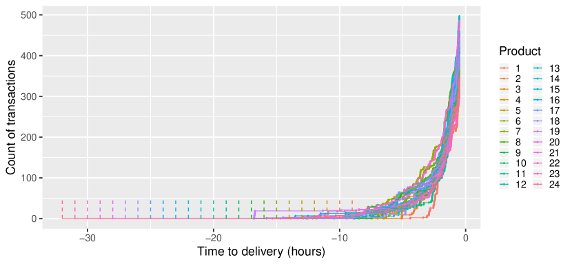
Figure 1: Trajectories of $S=24$ counting processes corresponding to transaction times for day $d=03.09.2017$ in the hourly German Intraday Continuous market. The dashed lines indicate the beginning of trading period $b(d,s)=-8-s$ of product $s\in\{1,\ldots,S\}$ with respect to the day of delivery $d$, the end of delivery $e(d,s)=0.5$.

The paper is structured as follows. In the next sections, we present the setting and the modelling details. Then, we explain the estimation and simulation methods. In the next section, we briefly describe the German Intraday Continuous market. In the sixth section, we introduce the forecasting study design, and we shortly present the exemplary dataset. Moreover, the evaluation measures are described. Next, the empirical forecasting results are presented. The paper is concluded with a discussion of the results and further development possibilities.

2 Setting

In the majority of all continuous intraday markets there are $S$ products traded each day, e.g. $S=24$ in a market with hourly products. For a certain day of delivery $d$ a product $s\in\{1,2,\dots,S\}$ is traded in the trading period $[b(d,s),e(d,s))$ prior to the beginning of the delivery. Here $b(d,s)$ denotes the beginning of the trading and $e(d,s)$ the end of the trading. Both $b(d,s)$ and $e(d,s)$ potentially depend on the day of trading $d$ and the considered product $s$. However, in the majority of European intraday markets the end of trading does not depend on the product $s$ but the beginning of trading does. Furthermore, if not mentioned otherwise all times are measured in hours.

During the trading period $[b(d,s),e(d,s))$ we observe a series of $n(d,s)$ intraday transaction times $\mathbb{T}^{d,s}=(T^{d,s}_{1},T^{d,s}_{2},\dots T^{d,s}_{n(d,s)})$ satisfying $b(d,s)<T^{d,s}_{1}$, $T^{d,s}_{i-1}<T^{d,s}_{i}$ for $i\in\{2,\ldots,n(d,s)\}$ and $T^{d,s}_{n(d,s)}<e(d,s)$. An example of trajectories of corresponding counting processes is presented in Figure 1 for $S=24$ products in the German Intraday Continuous market. As mentioned, the beginning of trading time differs for each product. For instance, the trading period in the German Intraday Continuous market for the hourly product $s=1$ with delivery starting at 00:00 is $[b(d,1),e(d,1))=[-9,-0.5)$ and for the hourly product $s=24$ with delivery starting at 23:00 is $[b(d,24),e(d,24))=[-32,-0.5)$.

Let us note that most of the transactions take place in the last hours of the trading period. The reason for this behaviour is the design of the intraday electricity market, i.e. its main purpose is to let the market participants react to the changes in production prediction. In the first hours of trading in the intraday market usually there is not much more information, when comparing to the day ahead market, but in the last hours before the delivery the difference is significant, and thus it is the most traded time period in this market. This pattern justifies the decision to parametrize the time in such a manner that the last hours of trading are indexed in the same way, disregarding the delivery time, as in Figure 1.

3 Modelling and estimation

In the purpose of estimating transaction arrivals, we consider the series of inter-arrival times $(X^{d,s}_{i})=(T^{d,s}_{i}-T^{d,s}_{i-1})$, where $i\in\{1,2,\dots,n(d,s)\}$, $n(d,s)$ is the number of transactions on day $d$ and product $s$ and $T_{0}^{d,s}=b(d,s)$ is the beginning of trading. As pointed out in Figure 1 only the latter hours of trading are of major interest for modelling. Hence, we focus on modelling only the part $[a(d,s),e(d,s))$ by choosing $a(d,s)$ such that $b(d,s)<a(d,s)<e(d,s)$. In the example Figure 1, a reasonable choice for $a(d,s)$ could be e.g. $-8$, $-5$ or $-3$. Denote $\mathbb{X}^{d,s}=(X^{d,s}_{i})$ all inter-arrival times after $a(d,s)$, so they satisfy $a(d,s)<T^{d,s}_{i}$. Further, let $l(d,s)$ be the smallest index such that $a(d,s)<T^{d,s}_{l(d,s)}$ holds.

Now, we assume that the series of inter-arrival times $\mathbb{X}^{d,s}$ is independent and follows a probability distribution with a parametric density function $f_{\mathbb{X}^{d,s}}(x;\theta)$. Therefore, knowing that the inter-arrival times are independent, we can perform the maximum likelihood estimation of the unknown vector of parameters $\theta$

$$\widehat{\theta}= \arg\max_{\theta}f_{\mathbb{X}^{d,s}}(x;\theta)=\arg\max_{\theta}\prod_{i=l(d,s)}^{n(d,s)}f_{\mathbb{X}^{d,s}}(x^{d,s}_{i};\theta).$$ (1)

Naturally, to make the estimation less biased, we can estimate the parameters using more than one day of history of the transaction arrival times. Assuming the independence between them and that we estimate based on $D$ days of history, we get the following maximum likelihood estimator

$$\widehat{\theta}= \arg\max_{\theta}f_{(\mathbb{X}^{1,s},\mathbb{X}^{2,s},\dots,\mathbb{X}^{D,s})}(x;\theta)$$ (2)

$$= \arg\max_{\theta}\prod_{d=1}^{D}f_{\mathbb{X}^{d,s}}(x;\theta)=\arg\max_{\theta}\prod_{d=1}^{D}\prod_{i=l(d,s)}^{n(d,s)}f_{\mathbb{X}^{d,s}}(x_{i}^{d,s};\theta).$$

The maximum likelihood problem stated in (2) is solved using Rsolnp package in R, which was implemented by Ghalanos and Theussl (2015), based on the algorithm of Ye (1987), which is the general non-linear augmented Lagrange multiplier method. Since the likelihood function may contain local maxima, it is very important to set correctly the lower and upper bounds and the starting parameters. The algorithm should handle with no big problem up to 10-parametric optimization, so in purpose of our study it is satisfactory. Nevertheless, the choice of the maximum likelihood optimization tool is not crucial as we have a low dimensional problem.

In the case of German Intraday Continuous market, we assume four distributions of the inter-arrival times: exponential, gamma, generalized gamma and generalized F. Each of the consecutive distributions is an extension of the previous one. The distributions are parametrized as follows:

• exponential distribution Exp($\lambda$) with rate parameter $\lambda>0$,

• gamma distribution Gamma($\alpha,\beta$) with shape and rate parameters $\alpha>0$ and $\beta>0$,

• generalized gamma distribution GenGam($\mu,\sigma,Q$) with location, scale and shape parameters $\mu\in\mathbb{R},\sigma>0$ and $Q\in\mathbb{R}$,

• generalized F distribution GenF($\mu,\sigma,Q,P$) with location and scale parameters $\mu\in\mathbb{R}$ and $\sigma>0$, and shape parameters $Q\in\mathbb{R}$ and $P\geq 0$.

The exponential and gamma distributions are well-know and thus do not need any special introduction. The exponential distribution has the following density function

$$f(x;\lambda)=\lambda\exp\{-\lambda x\}$$ (3)

and the gamma distribution has the density function defined by

$$f(x;\alpha,\beta)=\frac{\beta^{\alpha}}{\Gamma(\alpha)}x^{\alpha-1}\exp\{-\beta x\}.$$ (4)

Let us remind that the exponential distribution is a special case of the gamma distribution, i.e. if $X\sim\text{Exp}(\lambda)$, then $X\sim\text{Gamma}(\alpha=1,\beta=\lambda)$.

The generalized gamma distribution is an extension of the gamma distribution by Stacy et al. (1962), but in the study we use the parametrisation of Prentice (1974), which is stated above. If $\gamma\sim\text{Gamma}(Q^{-2},1)$ and $w=\log(Q^{2}\gamma)/Q$, then $x=\exp(\mu+\sigma w)$ follows the generalized gamma distribution with probability density function

$$f(x;\mu,\sigma,Q)=\frac{|Q|(Q^{-2})^{Q^{-2}}}{\sigma x\Gamma(Q^{-2})}\exp\{Q^{-2}(Qw-\exp\{Qw\})\}.$$ (5)

The relationship between the gamma and generalized gamma distributions parametrized in such a manner is as follows. If $X\sim\text{Gamma}(\alpha,\beta)$, then $X\sim\text{GenGam}(\mu=-\log(\beta/\alpha),\sigma=1/\sqrt{\alpha},Q=1/\sqrt{\alpha})$.

The last and the most general distribution that we assume is the generalized F distribution described by Prentice (1975). Define $s_{1}=2(Q^{2}+2P+Q\delta)^{-1}$ and $s_{2}=2(Q^{2}+2P-Q\delta)^{-1}$, where $\delta=(Q^{2}+2P)^{1/2}$. If $w=(\log(x)-\mu)\delta/\sigma$, then the probability density function of $x$ is given by

$$f(x;\mu,\sigma,Q,P)=\frac{\delta(s_{1}/s_{2})^{s_{1}}\exp\{s_{1}w\}}{\sigma x(1+s_{1}\exp(w)/s_{2})^{(s_{1}+s_{2})}B(s_{1},s_{2})},$$ (6)

where $B(s_{1},s_{2})$ is the beta function. Let us note that if we possess a random variable $X\sim\text{GenGam}(\mu,\sigma,Q)$, then $X\sim\text{GenF}(\mu,\sigma,Q,P=0)$. We see clearly that all the consecutive distributions are superior to the previous ones. Figure 2 presents densities of exemplary GenF distributions. In the exercise, we use the flexsurv package in R by Jackson (2016), which contains the implementation of the generalized gamma and F distributions.

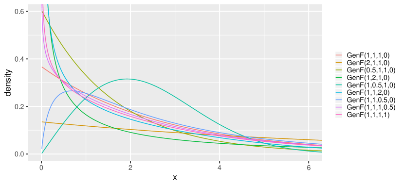
Figure 2: Illustration of the GenF distribution with different parameters

We assume that the rate parameter $\lambda$, the rate and shape parameters $\beta$ and $\alpha$, and the location and scale parameters $\mu$ and $\sigma$ are some deterministic functions dependent on time $t$ and unknown vector of parameters $\theta$. Thus, we model them using the following functions:

• constant — $f(t;\theta)=c$, where $\theta=c$,

• linear — $f(t;\theta)=c+\beta_{1}t$, where $\theta=(c,\beta_{1})$,

• quadratic — $f(t;\theta)=c+\beta_{1}t+\beta_{2}t^{2}$, where $\theta=(c,\beta_{1},\beta_{2})$,

• exponential — $f(t;\theta)=c+e^{\alpha_{1}+\alpha_{2}t}$, where $\theta=(c,\alpha_{1},\alpha_{2})$.

In the estimation of the parameters of generalized gamma and F distributions, we make use of the relationship between gamma and generalized gamma distributions, i.e. $\mu(\theta,t)=-\log(\beta(\theta_{2},t)/\alpha(\theta_{1},t))$ and $\sigma(\theta,t)=1/\sqrt{\alpha(\theta_{1},t)}$. Moreover, we assume that $\alpha(\theta_{1},t)$ cannot be more complex than $\beta(\theta_{2},t)$ and that the $Q$ and $P$ parameters are constant over time to delivery. By complexity of a function, we mean the number of parameters. Using this criteria, quadratic and exponential functions are equally complex.

The study consists in total of 37 models of the inter-arrival times process $\mathbb{X}^{d,s}$: 4 models with the assumption of the exponential distribution and 11 models per other considered distributions. We abbreviate them by X.Y.Z, where X stands for the distribution and Y and Z stand for the types of the $\beta(\theta_{2},t)$ and $\alpha(\theta_{1},t)$ functions, respectively. For instance, Gamma.Lin.Const stands for a model with assumed gamma distribution, linear $\beta(\theta_{2},t)$ and constant $\alpha(\theta_{1},t)$. Let us note that for the model with exponential distribution and $\lambda(\theta,t)=\theta$ the corresponding counting process is a homogeneous Poisson process and this model is our basic benchmark. Making the intensity function $\lambda(\theta,t)$ non-constant is the first extension of the benchmark and changing the distribution to the more general one is the further extension. Moreover, in this study for non-constant rate and shape functions we actually assume that the functions are constant in short intervals, e.g. for exponential distribution, $\lambda(\theta,T^{d,s}_{i})$ is assumed to be the intensity on the time interval $[T^{d,s}_{i},T^{d,s}_{i+1})$. This means that the corresponding counting process of a model with exponential distribution is a mixture of homogeneous Poisson processes.

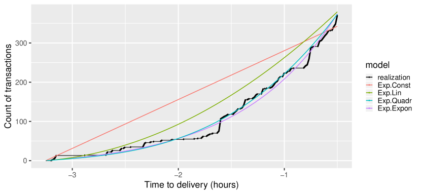
Figure 3: Observed trajectory of transaction counting process and fitted cumulative intensities of considered intensity functions of exponential distribution models for day $d=03.09.2017$ and product $s=12$ in the hourly German Intraday Continuous market

Let us note that the models contain not more than 8 parameters, so their estimation should not be a problem. Figure 3 shows an example of fitting the aforementioned models assuming the exponential distribution to one day of data for one product. The figure presents the observed trajectory and estimated cumulative intensity functions $\Lambda(B)=\int_{B}\lambda(t)dt$. The time to delivery range is $[a(d,s),e(d,s))=[-3.25,-0.5)$, because in this particular exercise we aim to forecast the transaction arrivals during the $\text{ID}_{3}$-Price period. This approach to the German Intraday Continuous was taken also by other researchers (Narajewski and Ziel, 2019; Uniejewski et al., 2019). Based on Figure 3, we may expect that considering the exponential distribution models, the models with quadratic and exponential intensity functions have similar performance in our problem.

4 Simulation

The trajectory simulation is relatively easy in our setting. Since we assume the distribution of the inter-arrival times $\mathbb{X}^{d,s}=(X^{d,s}_{i})$, we can simply generate the inter-arrival times from the estimated distribution and calculate the next arrival time by adding the simulated inter-arrival time to the time of forecasting. The only not that obvious part is the simulation of the first transaction arrival. That is to say, if we simulate at the time of the last observed transaction, there is no change, but if we fix the time of forecasting (e.g. like we do in the study), then we have to truncate the distribution for the first observation. This truncated distribution has the following density function

$$f_{\mathbb{X}^{d,s}}\left(\theta,x_{i}^{d,s}|X_{i}^{d,s}>y\right)=\frac{g(x_{i}^{d,s})}{1-F_{\mathbb{X}^{d,s}}(y)},$$ (7)

where $g(x)=f(x)$ for all $x>y$ and $g(x)=0$ otherwise, and $F_{\mathbb{X}^{d,s}}(y)$ is the cumulative distribution function of $\mathbb{X}^{d,s}$. All the next transaction arrivals are simulated using the standard distribution with the density function $f_{\mathbb{X}^{d,s}}$ at the simulated times $\widehat{T}_{j}$, where $j=i+1,i+2,\dots$ until the desired end of forecasting.

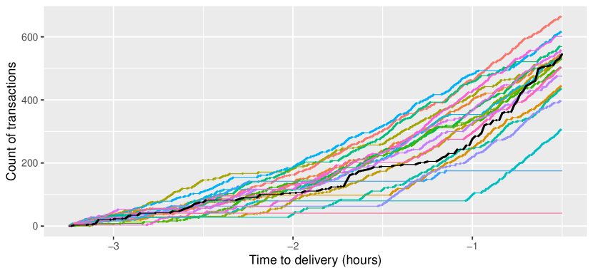
Figure 4: Observed (black) and simulated from the GenGam.Quadr.Expon (colourful) trajectories of transaction counting process for day $d=01.10.2017$ and product $s=18$ in the hourly German Intraday Continuous market

An example of simulation of 20 trajectories in the German Intraday Continuous market is shown in Figure 4. The trajectories are simulated as described above, based on the generalized gamma distribution with quadratic $\alpha(\theta_{1},t)$ and exponential $\beta(\theta_{2},t)$ functions, which was estimated using $D=28$ days of data.

5 German Intraday Continuous market

As mentioned, in the exemplary study we consider the German Intraday Continuous market. Trading in this market starts every day at 15:00 for hourly and at 16:00 for quarter-hourly products of the following day. Market participants can trade electricity until 30 minutes before the delivery in the whole market and until 5 minutes before the delivery in respective control zones. Figure 5 presents briefly the German electricity spot market, for more details see Viehmann (2017).

An important measure in the German Intraday Continuous market is the ID₃-Price index. The index is a volume-weighted price of all transactions taking place in the time interval between 3 hours and 30 minutes before the delivery and it is calculated separately for each intraday product. The importance of the ID₃-Price has been already noticed by the researchers and is a subject to modelling and forecasting by Uniejewski et al. (2019) and Narajewski and Ziel (2019). In the latter paper, one can find a broader description and analysis of the ID₃-Price and the German Intraday Continuous market. In both papers, the authors performed a very short-term point EPF of the ID₃-Price. The outcome of Narajewski and Ziel (2019) is the efficiency of the market, i.e. the volume-weighted price of the transactions in the last 15 minutes before forecasting appears to be the best model for the ID₃-Price. In our study, we aim to forecast the time arrivals during the ID₃-Price time interval. Naturally, we leave ourselves some time for calculation and decision-making and therefore the considered time frame is $[-3.25,-0.5)$ which is exactly the same as in Narajewski and Ziel (2019).

Figure 5: The daily routine of the German electricity market. $d$ corresponds to the day of the delivery and $s$ corresponds to the hour of the delivery.

In Europe the majority of intraday electricity markets features a similar structure to the German intraday market. This holds especially for all markets that participate in the Cross-Border Intraday Project (XBID), see e.g. Kath (2019). It allows various participating electricity markets (e.g. Germany, France, Spain) to bid across borders, if inter-connector capacity allows doing so. From the modelling perspective it might be relevant to note that all electricity markets which participate in XBID allow close their markets for each product the same amount of time before delivery, even though not always half an hour before delivery as in the German case. Thus, applying the modelling methodology to these markets should not be a problem.

6 Data, forecasting study and evaluation

In the following paper, as an example we perform a rolling window forecasting study based on the data from the German Intraday Continuous market. We consider a $D=28$-day window size with the initial in-sample data from 03.09.2017 to 30.09.2017 and forecast the next day arrivals, starting on 01.10.2017. We forecast the arrivals between 3 h 15 min and 30 min before the delivery. Our out-of-sample study is of size $N=365$, thus it spans the data range from 01.10.2017 to 30.09.2018. During each out-of-sample iteration $M=1000$ trajectories are simulated. In the study, a multivariate approach is taken, which means that we create 24 separate models, each for every hourly product.

The data that we utilize in the study was obtained from EEX Transparency, and it consists of information regarding: the date of the delivery, the product type, market area, volume of the traded energy, price in EUR/MWh, the transaction ID and the time of the transaction. In our case, the only relevant informations are the date of the delivery, the product type and of course the time of the transaction. A small inconvenience regarding the data is the fact that the transaction times have minute grid. This makes many transactions have identical time arrival even if they weren’t made at the same time, e.g. 4 transactions with timestamp of 30.09.2017 16:01:00. We deal with the problem by distributing the transactions with the same timestamp $T$ uniformly in the time range $[T,T+1\text{min})$. Using the aforementioned timestamp as an example, the new timestamps are: 30.09.2017 16:01:00, 16:01:15, 16:01:30, 16:01:45.

Due to the lack of literature regarding the intensity estimation in the intraday markets, we cannot use any literature benchmark models or literature evaluation measures. Thus, in the study we simply compare the results of simulation of all the considered models and as evaluation measures we use the functional: bias (Bias), mean absolute error (MAE), root mean squared error (RMSE) and continuous ranked probability score (CRPS). We abbreviate the functional measures in a standard way, but the calculation is a little different. That is to say, let us denote by $N^{d,s}(t)$ the counting process of the true transactions on day $d$ for product $s$ and by $N_{m}^{d,s}(t)$ the $m$-th simulation of the counting process $N^{d,s}(t)$.

Let

$$\rho_{\eta,\tau,p}(z)=(\eta z^{p}+(1-\eta)|z|^{p})|\tau-\mathds{1}(z<0)|$$

a loss function with $\eta\in\{0,1\}$, $\tau\in(0,1)$, $p\geq 1$ and $\mathds{1}$ as indicator function. Then we define

$$\widehat{N}^{d,s}_{\eta,\tau,p}(t)=\operatorname*{arg\,min}_{z}\sum_{m=1}^{M}\rho_{\eta,\tau,p}(N_{m}^{d,s}(t)-z)$$ (8)

the sample $\rho_{\eta,\tau,p}$-estimate of the corresponding simulation sample $N_{1}^{d,s},\ldots,N_{M}^{d,s}$. The special case $(\eta,\tau,p)=(0,0.5,2)$ in (8) corresponds to ordinary least squares (OLS) and $(\eta,\tau,p)=(0,0.5,1)$ to median regression. Thus, $\widehat{N}^{d,s}_{0,0.5,2}$ is the sample mean process, $\widehat{N}^{d,s}_{0,0.5,1}$ the sample median process and similarly $\widehat{N}^{d,s}_{0,\tau,1}$ the sample $\tau$-quantile process on which we focus especially. Now, we define the evaluation criteria

$$\text{EVAL}^{d,s}_{(\eta_{1},\tau_{1},p_{1}),(\eta_{2},\tau_{2},p_{2})}([T_{1},T_{2}))= \left(\int_{T_{1}}^{T_{2}}\rho_{\eta_{1},\tau_{1},p_{1}}(N^{d,s}(t)-\widehat{N}^{d,s}_{\eta_{2},\tau_{2},p_{2}}(t))dt\right)^{\frac{1}{p}}$$ (9)

$$= \left(\sum_{j=1}^{J}\rho_{\eta_{1},\tau_{1},p_{1}}(N^{d,s}(t_{j})-\widehat{N}^{d,s}_{\eta_{2},\tau_{2},p_{2}}(t_{j}))\Delta t_{j}\right)^{\frac{1}{p}}$$

on a time range $[T_{1},T_{2})$. $J$ is the length of a grid of the time range $[T_{1},T_{2})$ with $t_{0}=T_{1}$ and $t_{J}=T_{2}$. The grid is defined by the jumps of both of the counting processes. Let us note that the transition from the integral to the sum is possible, because the difference of counting processes is a simple function. Moreover, we approximate the values of the evaluation measures by using a minute grid instead of the one defined by the jumps to reduce computational costs.

Now, we define the special cases of the evaluation measures which lead to the functional bias (Bias), the functional MAE, functional RMSE and functional pinball (PB) loss (or quantile loss) with respect to a probability $\tau$:

$$\text{Bias}_{s} =\frac{1}{N}\sum_{d=1}^{N}2\text{EVAL}_{(1,0.5,1),(1,0.5,2)}^{d,s}$$ (10)

$$\text{MAE}_{s} =\frac{1}{N}\sum_{d=1}^{N}2\text{EVAL}_{(0,0.5,1),(0,0.5,1)}^{d,s}$$ (11)

$$\text{RMSE}_{s} =\frac{1}{N}\sum_{d=1}^{N}2\text{EVAL}_{(0,0.5,2),(0,.5,2)}^{d,s}$$ (12)

$$\text{PB}_{\tau,s} =\frac{1}{N}\sum_{d=1}^{N}\text{EVAL}_{(0,\tau,1),(0,\tau,1)}^{d,s}$$ (13)

We may observe that $2\text{PB}_{0.5,s}=\text{MAE}_{s}$. Additionally, we use the pinball loss to approximate the functional continuous ranked probability score (CRPS) by

$$\text{CRPS}_{s}=\frac{1}{R}\sum_{\tau\in r}\text{PB}_{\tau,s}$$ (14)

for an equidistant grid of probabilities $r$ between 0 and 1 of size $R$, see e.g. Nowotarski and Weron (2018). We consider the choice of $r=(0.01,0.02,\ldots,0.99)$ of size $R=99$. In the purpose of comparing the models’ forecasting performance, we calculate the functional Bias, MAE, RMSE and CRPS based on $M=1000$ trajectories in $N=365$ out-of-sample iterations and for all $s\in\{1,\ldots,S\}$ with $S=24$ products. For creating summaries, it may be useful to average across all products and define

$$\text{Crit}=\frac{1}{S}\sum_{s=1}^{S}\text{Crit}_{s}$$ (15)

for the considered criteria $\text{Crit}\in\{\text{Bias},\text{MAE},\text{RMSE},\text{PB}_{\tau},\text{CRPS}\}$.

To draw significant conclusions on the outperformance of the forecasts of the considered models, we also calculate the Diebold and Mariano (1995) test, which tests forecasts of model $A$ against forecasts of model $B$. In the following paper, we compute the multivariate version of the DM test as in Ziel and Weron (2018). The multivariate DM test results in only one statistic for each model that is computed based on the $S$-dimensional vector of losses for each day. Therefore, denote $L_{d}^{A}=(L^{A}_{d,1},L^{A}_{d,2},\dots,L^{A}_{d,S})^{\prime}$ and $L^{B}_{d}=(L^{B}_{d,1},L^{B}_{d,2},\dots,L^{B}_{d,S})^{\prime}$ the vectors of the out-of-sample losses for day $d$ of the models $A$ and $B$, respectively. By $L^{Z}_{d,s}$ we mean the CRPS_s loss for day $d$ of model $Z$, formally we choose

$$L^{Z}_{d,s}=\frac{1}{R}\sum_{\tau\in r}\text{EVAL}_{(0,\tau,1),(0,\tau,1)}^{Z,d,s}([T_{1},T_{2}))$$ (16)

with $[T_{1},T_{2})=[-3.25,-0.5)$. In the DM test we consider only the CRPS loss as it is the most important measure in our study. The multivariate loss differential series

$$\Delta^{A,B}_{d}=||L^{A}_{d}||_{q}-||L^{B}_{d}||_{q}$$ (17)

defines the difference of losses in $||\cdot||_{q}$ norm, i.e. $||L^{A}_{d}||_{q}=\left(\sum_{s=1}^{S}|L^{A}_{d,s}|^{q}\right)^{1/q}$, where $q\in\{1,2\}$ in our case. For each model pair, we compute the $p$-value of two one-sided DM tests. The first one is with the null hypothesis $\mathcal{H}_{0}:\mathbb{E}(\Delta_{d}^{A,B})\leq 0$, i.e. the outperformance of the forecasts of model B by the forecasts of model A. The second test is with the reverse null hypothesis $\mathcal{H}_{0}^{R}:\mathbb{E}(\Delta_{d}^{A,B})\geq 0$, i.e. the outperformance of the forecasts of model A by those of model B. Let us note that these tests are complementary, and we perform them using two norms – $||\cdot||_{1}$ and $||\cdot||_{2}$. Naturally, we assume that the loss differential series is covariance stationary.

7 Results

	Bias	MAE	RMSE	CRPS
Exp.Const	144.113	220.132	155.464	100.161
Exp.Lin	1.703	151.349	114.710	67.504
Exp.Quadr	-28.784	142.488	108.482	63.410
Exp.Expon	-40.138	138.866	105.592	61.761
Gamma.Const.Const	156.004	225.793	158.639	100.991
Gamma.Lin.Const	-0.785	150.973	114.573	66.631
Gamma.Lin.Lin	24.151	163.237	123.187	72.023
Gamma.Quadr.Const	-28.934	142.568	108.524	62.857
Gamma.Quadr.Lin	-26.498	143.301	108.908	62.413
Gamma.Quadr.Quadr	-29.339	146.516	111.385	64.006
Gamma.Quadr.Expon	-22.970	145.052	110.128	63.170
Gamma.Expon.Const	-40.136	138.952	105.607	61.218
Gamma.Expon.Lin	-36.848	138.829	105.448	60.427
Gamma.Expon.Quadr	-40.102	139.659	105.957	60.770
Gamma.Expon.Expon	-41.907	139.741	106.098	60.845
GenGam.Const.Const	152.901	252.987	164.072	90.424
GenGam.Lin.Const	72.961	189.489	129.545	68.444
GenGam.Lin.Lin	-17.116	160.708	118.308	60.203
GenGam.Quadr.Const	67.173	188.348	129.674	68.624
GenGam.Quadr.Lin	-52.039	161.245	123.312	62.396
GenGam.Quadr.Quadr	-62.730	165.170	126.515	64.582
GenGam.Quadr.Expon	-63.908	153.412	118.432	58.893
GenGam.Expon.Const	69.276	190.731	130.242	69.003
GenGam.Expon.Lin	16.182	174.413	124.556	64.196
GenGam.Expon.Quadr	-59.219	156.238	120.499	59.710
GenGam.Expon.Expon	-0.735	173.996	125.897	64.519
GenF.Const.Const	77.112	216.268	146.789	75.662
GenF.Lin.Const	8.387	170.659	124.043	61.562
GenF.Lin.Lin	-54.312	163.464	126.611	61.717
GenF.Quadr.Const	4.748	170.497	124.345	61.797
GenF.Quadr.Lin	-101.139	167.424	134.291	64.764
GenF.Quadr.Quadr	-102.141	172.586	137.630	68.198
GenF.Quadr.Expon	-109.600	164.070	132.864	63.636
GenF.Expon.Const	8.630	173.305	125.668	62.511
GenF.Expon.Lin	-39.876	168.606	128.455	62.641
GenF.Expon.Quadr	-106.988	164.796	133.924	63.842
GenF.Expon.Expon	-41.044	172.291	130.456	63.797

Table 1: Bias, MAE, RMSE and CRPS for the considered models on the interval $[T_{1},T_{2})=[-3.25,-0.5)$. Bolded values indicate the lowest value in each column, instead of bias, where it indicates the value closest to 0.

Table 1 presents the Bias, MAE, RMSE and CRPS measures (see equation(15) ) of the considered models on the interval $[T_{1},T_{2})=[-3.25,-0.5)$ which was used for estimation. In the table, we observe that the lowest MAE and RMSE are obtained for model Gamma.Expon.Lin. At the same time we see that the values for the other models with gamma distribution and exponential rate function have similar performance, as well as model Exp.Expon, which appears to be the second best in terms of MAE and RMSE. These values indicate that most likely the difference in the performance of modelling the median and mean of models Gamma.Expon.Lin and Exp.Expon is not statistically significant. The models with generalized gamma and generalized F distributions clearly have difficulties in modelling the central parts of the distribution, but they handle the probabilistic forecasting well. The best performing model in terms of CRPS is GenGam.Quadr.Expon. The CRPS values of other models are mostly satisfying despite the models with constant parameters. These give the worst forecasts in terms of all considered measures.

On the other hand, the values of bias are interesting. We see there that the best models underestimate the true counting process. The reason for such an underestimation may be the fact that the German Intraday Continuous is constantly developing and the number of trades is growing every day. This suggests that there is still some space for improvement of the errors. In the remaining part of this section, we consider only selected best performing models: 2 best models per distribution and from each of the distributions, we choose also the best model with exponential rate function.

(a)

(b)

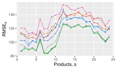
(c)

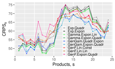
(d)

Figure 6: (a) Bias_s, (b) MAE_s, (c) RMSE_s and (d) CRPS_s of selected best performing models evaluated on $[T_{1},T_{2})=[-3.25,-0.5)$.

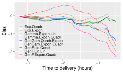
(a)

(b)

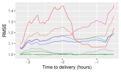
(c)

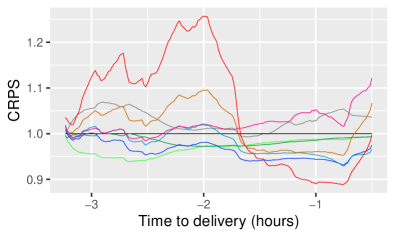
(d)

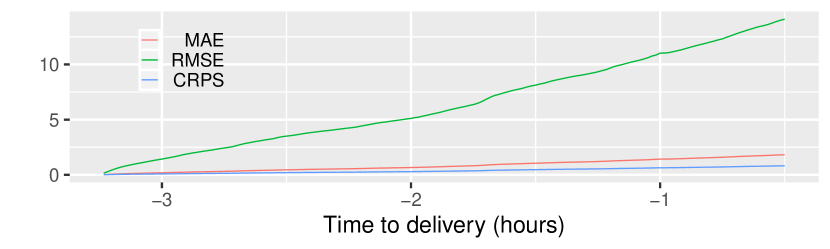
(e)

Figure 7: (a) Bias of the selected models, (b) MAE, (c) RMSE, (d) CRPS measures of selected best performing models in relation to the values of the model Exp.Expon and (e) errors of Exp.Expon over time to delivery.

Figure 6 contains four graphs that present the performance of the selected models’ forecasts over products $s\in\{1,\ldots,S\}$. In Figure 6a, we observe that all the models despite the GenF.Lin.Const underestimate the true trajectory for all products. There is no clear pattern of the underestimation, but we see that the bias of best models in terms of MAE and RMSE is almost constant over products, whereas the bias of the best model in terms of CRPS varies significantly. Figures 6b, 6c and 6d show that all models handle the simulation of night hours’ transactions better than the simulation of the day hours’. An interesting spike in both measures can be observed for $s=6$. The reason for that might be some outliers as the spike is higher in terms of RMSE than in terms of MAE or CRPS. Furthermore, we see that the models with exponential and gamma distribution are clearly better than the others across all products in terms of MAE and RMSE. It is different for CRPS, where for most hours the best models are the GenGam models, but between hours 6 and 10 the gamma distributed models appear to be better.

Figure 7 is analogous to Figure 6, but the measures are calculated over the time to delivery. This means that we calculate the values (see equation (15)) on many short time intervals, i.e. we apply a minute grid of the time-frame $[-3.25,-0.5)$. This way we can understand which part of the trajectory is forecasted the most and the least precisely. Figure 7a shows that the most underestimated is the last 1.5 hour of the counting process, but the models with gamma and exponential distribution handle this period better than the GenGam and GenF models. Figures 7b and 7c show again the Gamma and Exp models with exponential rate function give mostly the lowest MAE and RMSE. In Figure 7d, we see that Gamma.Expon.Lin model has lowest CRPS in the first half of the forecasting horizon and, surprisingly, in the second half the lowest CRPS value is obtained for model GenF.Lin.Const. The performance of GenGam.Quadr.Expon is mostly stable over the time to delivery. Figure 8 shows the pinball loss results of the models over probability values. Based on it, it is clear that the Gamma and Exp models forecast better the central quantiles, i.e. between 0.2 and 0.7, whereas the others are better forecasted by GenGam and GenF models. The figure indicates that the overall CRPS performance can be significantly improved.

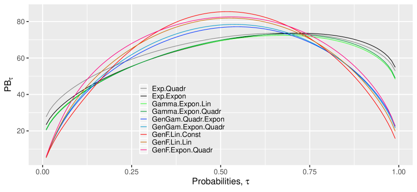
Figure 8: PB_τ of selected best performing models over probabilities $\tau\in\{0.01,0.02,\ldots,0.99\}$.

(a)

(b)

Figure 9: Results of the Diebold-Mariano test. (a) presents the $p$-values for the $||\cdot||_{1}$ norm with the CRPS loss, (b) the values for the $||\cdot||_{2}$ norm with the CRPS loss. The figures use a heat map to indicate the range of the $p$-values. The closer they are to zero ($\to$ dark green), the more significant the difference is between forecasts of X-axis model (better) and forecasts of the Y-axis model (worse).

To draw statistically significant conclusions, we perform a Diebold-Mariano test. The results are presented in Figure 9. Let us remind that we use the CRPS as the loss series as we believe that it is the most important measure in this study. Based on it, it is clear that the GenGam.Quadr.Expon model is significantly the best. Interestingly, the test in norm $||\cdot||_{2}$ indicates a very good performance of the GenF models. Although, in this norm none of the other models is significantly better than the GenGam.Quadr.Expon.

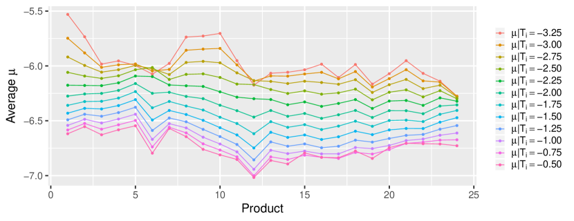
(a)

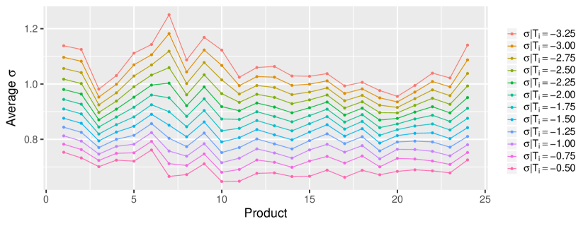
(b)

Figure 10: Average (a) location $\mu$ and (b) scale $\sigma$ parameters of model GenGam.Quadr.Expon over products at time $T_{i}\in\{-3.25,-3,\dots,-0.5\}$

Let us now take a look at the values of the time-varying coefficients of the model GenGam.Quadr.Expon. Let us recall that in this model we estimate the inter-arrival time $X_{i}^{d,s}$ assuming generalized gamma distribution with the time-varying coefficients $\mu(\theta,t)=-\log(\beta(\theta_{2},t)/\alpha(\theta_{1},t))$ and $\sigma(\theta,t)=1/\sqrt{\alpha(\theta_{1},t)}$ and constant $Q$, where $\beta(\theta_{2},t)$ and $\alpha(\theta_{1},t)$ are the rate and shape parameters of the standard gamma distribution. In this model $\beta(\theta_{2},t)$ is a quadratic function and $\alpha(\theta_{1},t)$ is an exponential function. In Figure 10, we analyse the behaviour of $\mu$ and $\sigma$ parameters over products at different time. Figure 10a shows that the values of $\mu$ are similar over products, but differ significantly over time. That is to say, the closer we are to the gate closure, the lower the location coefficient, which means that the transactions appear more often. Figure 10b shows a very similar behaviour for the scale parameter $\sigma$. In this case the closer we are to the gate closure, the less vary the inter-arrival times.

8 Conclusion

We described the novel problem of estimation and simulation of the transaction arrival process in intraday electricity markets. The approach is not complicated and the presented methods are easy to implement. The paper fills the gap in the literature regarding the estimation and simulation of the transaction arrival process in the intraday electricity markets and thus is a major contribution to this field of research. The outcome of the conducted study is very satisfying.

Using the aforementioned approach, we utilized an exemplary rolling window forecasting study based on the German Intraday Continuous market. We assumed four probability distributions of the inter-arrival times: exponential, gamma, generalized gamma and generalized F distributions. We performed the maximum likelihood estimation of the distributions, assuming time-dependence of some of their coefficients. Then, using the estimated distributions we simulated new trajectories which we evaluated using the functional bias, MAE, RMSE and CRPS.

The results showed that the forecasting error can be significantly reduced, comparing to the most standard benchmark, which was the homogeneous Poisson process. The best in terms of forecasting of the central part of the distribution of the transaction arrivals, i.e. the mean or median are the exponential and gamma distributions with exponential rate function. In terms of the more meaningful and thus more important CRPS significantly the best forecasts were obtained from the generalized gamma model with quadratic rate function and exponential shape function.

This field of research can be easily developed further. A possible direction is considering other probability distributions of the inter-arrival times. Another possibility would be using more complex distributions’ parameter functions, e.g. Hawkes process-like, which is widely applied to modelling the transaction time arrivals in the financial markets, see e.g. Hewlett (2006) or Bacry et al. (2015). The parameter functions could be also modelled using smoothing kernel or splines. To avoid overestimation, regularization methods should be considered.

References

- Aïd et al. (2016) Aïd, R., P. Gruet, and H. Pham (2016). An optimal trading problem in intraday electricity markets. Mathematics and Financial Economics 10(1), 49–85.
- Andrade et al. (2017) Andrade, J. R., J. Filipe, M. Reis, and R. J. Bessa (2017). Probabilistic Price Forecasting for Day-Ahead and Intraday Markets: Beyond the Statistical Model. Sustainability 9(11), 1990.
- Bacry et al. (2015) Bacry, E., I. Mastromatteo, and J.-F. Muzy (2015). Hawkes processes in finance. Market Microstructure and Liquidity 1(01), 1550005.
- Diebold and Mariano (1995) Diebold, F. and R. Mariano (1995). Comparing Predictive Accuracy. Journal of Business & Economic Statistics 13(3), 253–63.
- Diebold (2015) Diebold, F. X. (2015). Comparing predictive accuracy, twenty years later: A personal perspective on the use and abuse of diebold–mariano tests. Journal of Business & Economic Statistics 33(1), 1–1.
- Ghalanos and Theussl (2015) Ghalanos, A. and S. Theussl (2015). Rsolnp: General Non-linear Optimization Using Augmented Lagrange Multiplier Method. R package version 1.16.
- González-Aparicio and Zucker (2015) González-Aparicio, I. and A. Zucker (2015). Impact of wind power uncertainty forecasting on the market integration of wind energy in spain. Applied energy 159, 334–349.
- Graf von Luckner et al. (2017) Graf von Luckner, N., Á. Cartea, S. Jaimungal, and R. Kiesel (2017). Optimal market maker pricing in the german intraday power market.
- Hewlett (2006) Hewlett, P. (2006). Clustering of order arrivals, price impact and trade path optimisation. In Workshop on Financial Modeling with Jump processes, Ecole Polytechnique, pp. 6–8.
- Jackson (2016) Jackson, C. H. (2016). flexsurv: a platform for parametric survival modeling in r. Journal of Statistical Software 70.
- Kath (2019) Kath, C. (2019). Modeling intraday markets under the new advances of the cross-border intraday project (xbid): Evidence from the german intraday market. Energies 12(22), 4339.
- Kiesel and Paraschiv (2017) Kiesel, R. and F. Paraschiv (2017). Econometric analysis of 15-minute intraday electricity prices. Energy Economics 64, 77–90.
- Kulakov and Ziel (2019) Kulakov, S. and F. Ziel (2019). The impact of renewable energy forecasts on intraday electricity prices. arXiv preprint arXiv:1903.09641.
- Monteiro et al. (2016) Monteiro, C., I. J. Ramirez-Rosado, L. A. Fernandez-Jimenez, and P. Conde (2016). Short-Term Price Forecasting Models Based on Artificial Neural Networks for Intraday Sessions in the Iberian Electricity Market. Energies 9(9), 721.
- Narajewski and Ziel (2019) Narajewski, M. and F. Ziel (2019). Econometric modelling and forecasting of intraday electricity prices. Journal of Commodity Markets, 100107.
- Nowotarski and Weron (2018) Nowotarski, J. and R. Weron (2018). Recent advances in electricity price forecasting: A review of probabilistic forecasting. Renewable and Sustainable Energy Reviews 81, 1548–1568.
- Pape et al. (2016) Pape, C., S. Hagemann, and C. Weber (2016). Are fundamentals enough? explaining price variations in the german day-ahead and intraday power market. Energy Economics 54, 376–387.
- Prentice (1974) Prentice, R. L. (1974). A log gamma model and its maximum likelihood estimation. Biometrika 61(3), 539–544.
- Prentice (1975) Prentice, R. L. (1975). Discrimination among some parametric models. Biometrika 62(3), 607–614.
- Stacy et al. (1962) Stacy, E. W. et al. (1962). A generalization of the gamma distribution. The Annals of mathematical statistics 33(3), 1187–1192.
- Uniejewski et al. (2019) Uniejewski, B., G. Marcjasz, and R. Weron (2019). Understanding intraday electricity markets: Variable selection and very short-term price forecasting using lasso. International Journal of Forecasting.
- Viehmann (2017) Viehmann, J. (2017, Jun). State of the German Short-Term Power Market. Zeitschrift für Energiewirtschaft 41(2), 87–103.
- Ye (1987) Ye, Y. (1987). Interior Algorithms for Linear, Quadratic, and Linearly Constrained Non-Linear Programming. Ph. D. thesis, Department of ESS, Stanford University.
- Ziel (2017) Ziel, F. (2017). Modeling the impact of wind and solar power forecasting errors on intraday electricity prices. In 2017 14th International Conference on the European Energy Market (EEM), pp. 1–5. IEEE.
- Ziel and Weron (2018) Ziel, F. and R. Weron (2018). Day-ahead electricity price forecasting with high-dimensional structures: Univariate vs. multivariate modeling frameworks. Energy Economics 70, 396–420.