How ill-defined constituents produce well-defined nanoparticles: Effect of polymer dispersity on the uniformity of copolymeric micelles

Abstract

We investigate the effect of polymer length dispersity on the properties of self-assembled micelles in solution by self-consistent field calculations. Polydispersity stabilizes micelles by raising the free energy barriers of micelle formation and dissolution. Most importantly, it significantly reduces the size fluctuations of micelles: Block copolymers of moderate polydispersity form more uniform particles than their monodisperse counterparts. We attribute this to the fact that the packing of the solvophobic monomers in the core can be optimized if the constituent polymers have different length.

Polymeric nanoparticles are attracting considerable and growing interest because of their potential in materials science Bucaro et al. (2009); Ethirajan and Landfester (2010); Nasir et al. (2015) and in nanomedicine, e.g., in targeted therapeutic or diagnostic systems Ulbrich et al. (2016); Tibbitt et al. (2016). One attractive way to fabricate such nanoparticles is to exploit the self-assembly of amphiphilic block copolymers in solution. Depending on the lengths and solubilities of the copolymer blocks, they can form a variety of interesting morphologies, such as vesicles, rods, and spherical micelles Förster and Plantenberg (2002); Rodriguez-Hernandez et al. (2005).

In the present article, we consider the micelles, which have a core-shell structure with a solvophobic core and a solvophilic shell exposed to the solventLeermakers et al. (1995); Webber (1998); Riess (2003). In principle, the core can be exploited to load the drug molecules, and efficient mechanisms can be devised to enhance bioavailability Lebouille et al. (2013); Feng et al. (2014); Nakayama and Okano (2006). As long as the drug is stably encapsulated, it is believed that the distribution of drug-loaded polymeric micelles in the body is determined by the size and surface properties of polymeric micelles rather than the properties of the drug moleculesKataoka et al. (2001); Cabral et al. (2011); Chang et al. (2014). Hence developing strategies to control the size distribution of polymeric micelles is important to improve the efficacy of targeted drug delivery techniques.

However, all synthetic polymers, including block copolymers, possess some inherent dispersity in the polymer length due to the nature of polymerization reactionSeno et al. (2007); Lynd et al. (2008); Doncom et al. (2017). Currently, it is not understood to which extent the polydispersity of block copolymers affects the dispersity of the formed micelles – especially since even monodisperse amphiphiles do not form monodisperse micelles Nelson et al. (1997). Polydisperse polymer systems contain individual polymers with shorter or longer blocks. This provides an entropic advantage in the self-assembly process, since long chains can fill the center of domains without having to stretch, whereas short chains adopt conformations near the interfaceLynd et al. (2008); Doncom et al. (2017). Indeed, experiments on ABA triblock copolymer melts have indicated that polydispersity greatly enhances the stability of self-assembled lamellar structures Widin et al. (2012). Related observations have been made in theoretical studies of polymer brushes: They indicate that monodisperse brushes show multicritical behavior Qi et al. (2016); Romeis and Sommer (2015), which are associated with large anomalous chain fluctuations Skvortsov et al. (1997); Merlitz et al. (2008); Romeis and Sommer (2013) that disappear in polydisperse brushes Qi et al. (2016). Hence it is not a priori clear whether polydispersity will enhance or reduce the size fluctuations of self-assembled micelles.

This question is addressed in the present article. We use self-consistent field (SCF) theory to study the structures and free energy landscapes of micelles that assemble from polydisperse polymer solutions for varying polydispersity index (Đ) close to the critical micelle concentration (CMC), i.e., the point where micelles just begin to form.

Studies of polydispersity effects on self-assembled nanostructures are still comparatively scarce (for reviews see Lynd et al. (2008); Doncom et al. (2017)). Most studies have considered polydispersity effects on the self-organization in block copolymer melts Nguyen et al. (1994); Matsushita et al. (2003); Sides and Fredrickson (2004); Noro et al. (2005); Wang et al. (2005); Ruzette et al. (2006); Torikai et al. (2006); Lynd and Hillmyer (2005, 2007); Lynd et al. (2007, 2008); Park et al. (2008); Matsen (2006, 2007); Cooke and Shi (2006); Oschmann et al. (2017). Early theoretical studies Gao and Eisenberg (1993); Linse (1994) on micellar solutions have predicted that the CMC decreases with polydispersity Gao and Eisenberg (1993) and that the polymers in the micelles are on average longer than in the surrounding solution. This was later confirmed by experiments Khougaz et al. (1994); Hvidt et al. (2002). The size of vesicles formed by amphiphilic diblock copolymers in solution was reported to decrease with increasing dispersity of the hydrophilic blockTerreau et al. (2003); Jiang et al. (2005); Li et al. (2009). In contrast, experimental studies on micelles made of amphiphilic triblocks with polydisperse inner (hydrophobic) block have shown that the micelle sizes may increase significantly with Đ (at comparable average chain length) Schmitt et al. (2012), in agreement with theoretical predictions Linse (1994), and that micelles may even become slightly oblate for high polydispersities Schmitt et al. (2012). The latter effect is however small (the aspect ratio is 1:1.4), and since we focus on moderate polydispersities in the present work, we will assume that micelles are spherically symmetric.

Model and Method. We study systems of polydisperse amphiphilic diblock copolymers with solvophobic blocks A (chain fraction f) and solvophilic blocks B (chain fraction (1-f)) immersed in a solvent S, in the grand canonical ensemble. Since every copolymer length $N$ defines a separate species, we must introduce separate chemical potentials $\mu_{P}(N)$ for each. They are adjusted such that copolymers in solution are distributed according to a Schulz-Zimm distribution Fredrickson and Sides (2003) $P_{SZ}(N)$ with average chain length $N_{n}=\sum_{N}\>N\>P_{SZ}(N)$ and polydispersity index Đ$=\sum_{N}\>N^{2}P(N)/N_{n}^{2}$. Note that the chain length distribution in the micelles may differ from $P_{SZ}(N)$.

Polymers are modeled as flexible Gaussian chainsDoi and Edwards (1986); Fredrickson (2006). The segment interactions are characterized by Flory-Huggins parameters $\chi_{ij}N_{n}$ ($i,j=A,B,S$) and are chosen similar to previous workHe and Schmid (2006) as $\chi_{AB}N_{n}=10.0$, $\chi_{AS}N_{n}=17.4$ and $\chi_{BS}N_{n}=-0.5$. The system is compressible with compressibility (Helfand) parameter $\kappa_{H}N_{n}=100$. The structure and the free energy of spherically symmetric micelles are calculated within the SCF theory Helfand (1975); Schmid (1998); Fredrickson (2006). The model equations, model parameters, and further details are given in SI. The micelle free energy $F_{m}$ is obtained from the free energy difference of a system containing a micelle and the corresponding (”bulk”) homogeneous system. The micelle radius is defined as the radius where the solvophobic density assumes the value $\Phi_{A}=0.5$. In the following, spatial distances are reported in units of radius of gyration ($\bar{R}_{g}$) of ideal Gaussian chains with length $N_{n}$ ($\bar{R}^{2}_{g}=\frac{N_{n}b^{2}}{6}$), densities are made dimensionless by dividing them by the bulk segment density $\rho_{0}$, and energies are given in units of $\bar{C}k_{B}T$, where $\bar{C}=\bar{R}^{3}_{g}\rho_{o}/N_{n}$, is the Ginzburg parameter which characterizes the strength of fluctuations in the system Schmid (2011); Fredrickson (2006). In the present article, we consider block copolymers with A- and B-blocks of equal average molecular weight ($\langle f\rangle=0.5$), as in the experimental system of Ref. Schmitt et al. (2012).

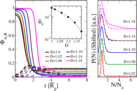
Figure 1: Left: Spatial density profiles of solvophobic A segments (full lines) and solvophilic B segments (dashed lines) in micelles made of A:B copolymers with f=0.5, ${\color[rgb]{0,0,0}F_{m}/k_{B}T\approx 0}$ for different bulk polydispersity indices Đ as indicated. Inset shows the corresponding shift of the polymer volume fraction $\bar{\Phi}_{p}$ in the bulk. Right: Chain length distribution of copolymers in the bulk (dashed) and in the micelle (solid) for different values of Đ. A constant offset has been added for better visibility.

Micelle structures and size distributions. We first consider copolymers with fixed block ratio $f=0.5$. We compare systems with same average chain length in the bulk and same micelle free energy $F_{m}/k_{B}T\approx 0$ (where micelles just begin to form), but varying polydispersity index Đ. To fix $F_{m}$, the bulk polymer volume fraction $\bar{\Phi}_{p}$ must be adjusted. We find that $\bar{\Phi}_{P}$ decreases significantly with Đ (Fig. 1, inset), indicating that micelle formation sets in for smaller copolymer concentrations in polydisperse solutions. Moreover, the micelle size increases with Đ (Fig. 1, left). The reason becomes clear when examining the chain length distribution in the micelles (Fig. 1, right). In polydisperse systems, it differs significantly from the chain length distribution in the bulk. The largest chains in solution aggregate first, presumably because they can form aggregates at lower cost of translational entropy, hence micelles become bigger. These effects are in agreement with earlier theoretical predictions Gao and Eisenberg (1993); Linse (1994) and experimental results Hvidt et al. (2002); Schmitt et al. (2012). Similar effects are observed for critical nuclei in polymer mixtures Qi and Yan (2008).

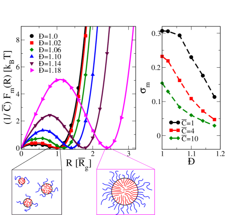
Figure 2: Left: Micelle free energy as a function of micelle radius for the same systems as in Fig. 1. Symbols show SCF results, solid lines a fit to the polynomial $\sum_{n=1}^{4}a_{n}x^{n}$. Right: Corresponding micelle size dispersity $\sigma_{m}$ as a function of copolymer polydispersity index Đ for different values of the scaling parameter $\bar{C}$. Cartoons illustrate the proposed stabilizing mechanism: Polydisperse solvophobic blocks can pack more efficiently in the core of the micelle.

Next we study the size distribution of micelles. To this end, we determine the constrained free energy $F_{m}(R)$ for micelles of fixed radius $R$ (see SI for technical details). The probability for finding a micelle with size $R$ is then proportional to $\exp(-F_{m}(R)/k_{B}T)$. The function $F_{m}(R)$ is shown in Fig. 2(left). It starts at $F_{m}(0)=0$, then exhibits a maximum followed by a minimum. The minimum corresponds to the most probable micelle size $R_{mp}$ and coincides with the solution of the unconstrained SCF equations discussed above (Fig. 1). Consistent with Fig. 1, it shifts to the right with increasing polymer polydispersity. The maximum correspond to an unstable micelle state: micelles of this size may dissolve again. We will refer to it as critical micelle size $R_{mc}$. The height of the maximum gives the free energy barrier for micelle formation, and the free energy difference $\Delta F_{m}=F_{m}(R_{mc})-F_{m}(R_{mp})$ gives the free energy barrier for micelle dissolution. According to Fig. 2, these barriers increase with increasing polydispersity. Hence polydispersity stabilizes micelles, suggesting that they might also have narrower size distributions.

The micelle size dispersity is characterized by the relative width of the size distribution, $\sigma_{m}=\sqrt{\langle R^{2}\rangle/\langle R\rangle^{2}-1}$. To calculate $\sigma_{m}$, we fit the SCF results for $F_{m}(R)$ to a fourth order polynomial (see Fig. 2, left) and use that to determine the averages $\langle R^{k}\rangle=I_{k}/I_{0}$ with $I_{k}=\int_{R_{mc}}^{\infty}{\rm d}R\>R^{k}\>{\rm e}^{-F_{m}(R)/k_{B}T}$. In doing so, we must specify a value for the global prefactor $\bar{C}$ in $F_{m}(R)$ (see Fig. 2, left). The Ginzburg $\bar{C}$ is related to a complementary parameter called the invariant polymerisation index ($\bar{N}$) as, $\bar{N}\propto\bar{C}^{2}$, where $\bar{N}=N_{n}\rho^{2}_{0}b^{6}$. Typical values for $\bar{N}$ in experimental systems areGlaser et al. (2014); Bates et al. (1994, 1990, 1988) $\bar{N}\simeq 200-20000$, which corresponds to $\bar{C}\simeq 1-10$. Fig. 2 (right) shows our results for $\sigma_{m}$ as a function of Đ for three different choices ${\color[rgb]{0,0,0}\bar{C}}=1,4$, and $10$. In all cases, the micelle size dispersity $\sigma_{m}$ decreases with increasing polymer dispersity Đ. Thus we find that polymer dispersity not only stabilizes micelles, but also reduces their size dispersity. This is the main result of the present article.

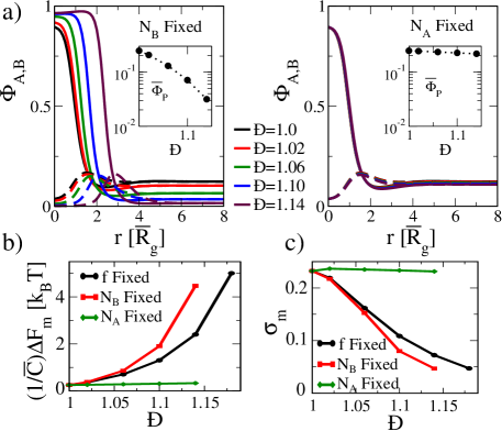
Figure 3: (a) Density profiles of A and B segments (full/dashed lines) for micelles with micelle free energy $\Delta F_{m}=0$ in systems where only the solvophobic (left) or solvophilic (right) chain block is polydisperse. The inset shows the corresponding bulk polymer volume fractions $\bar{\Phi}_{P}$. (b) Height $\Delta F_{m}$ of the free energy barrier for micelle dissolution. (c) Width $\sigma_{m}$ of micelle size distribution at $\bar{C}=4$ vs. Đ for all systems considered in the present work. Here  Đ refers to the dispersity in the corresponding polydisperse part of the chain (A or B or total).

Other copolymer architectures. To further investigate this phenomenon, we study two other classes of systems where the copolymer blocks still have equal length on average ($\langle f\rangle=0.5$), but are now varied independently: In the first system, ths solvophobic block is polydisperse with ${\left<N_{A}\right>}/{N_{n}}=0.5$ and the length of the solvophilic block is kept fixed at ${N_{B}}/{N_{n}}=0.5$. In the second system, the solvophobic block is fixed at ${N_{A}}/{N_{n}}=0.5$ and the length of the solvopholic block fluctuates with ${\left<N_{B}\right>}/{N_{n}}=0.5$.

The main results of the SCF calculations are compiled in Fig. 3. If only the solvophobic block is polydisperse and the solvophilic block is kept monodisperse, the effect of polydispersity on the micelle size (Fig. 3 a), left), the chain length distribution (Fig. S2 in SI), the height of the free energy barrier $\Delta F_{m}$ (Fig. 3 b) and the micelle dispersity (Fig. 3 c) is even stronger than before. In contrast, if the solvophobic block is monodisperse, polydispersity of the solvophilic block has almost no influence on the micelle size (Fig. 3(a), right) and the other micelle characteristics. Hence the micelle structure and size distribution in the solution is primarily determined by the dispersity of the solvophobic chain block. These results suggest that the main effect of polydispersity is to enhance the packing efficiency inside the hydrophobic core.

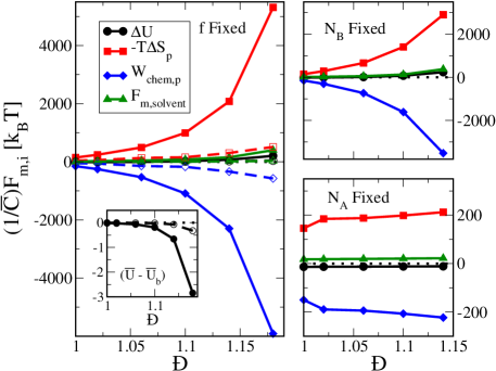
Figure 4: Contributions to the micelle free energies from the interaction energy (black circles), the polymer entropy (red squares), the chemical work associated with the polymers (blue diamonds) and the sum of solvent entropy and solvent chemical work (green triangles), for the systems considered in this work. Full lines/full symbols refer to most probable micelles, dashed lines/open symbols to critical micelles. Inset shows the difference between the internal energy per polymer segment in the micelle system and in the bulk (in arbitrary units).

Free energy analysis. To test this hypothesis, we separate the different contributions to the micelle free energy according to $F_{m}=\Delta U+W_{\mbox{\tiny chem}}-T\Delta S$, where $\Delta U$ and $\Delta S$ are the interaction energy and entropy in the micelle relative to the bulk, and $W_{\mbox{\tiny chem}}=-\mu_{s}\Delta n_{s}-\sum_{N}\mu_{p}(N)\Delta n_{P}(N)$ refers to the chemical work required for bringing polymer into the system and moving solvent out ($\Delta n_{x}$ is the excess number of molecules of type $X$ in the micelle). Within the SCF framework, the contributions of polymers and solvent to the entropy and the chemical work can be calculated separately (see SI for technical details). The results are shown in Fig. 4. The dominant terms are the polymer entropy and the chemical work associated with the polymers.

The polymer entropy decreases with increasing polydispersity Đ. This supports the packing hypothesis: Well-packed polymers fluctuate less and explore fewer conformations, which reduces their entropy. Interestingly, micelle formation in polydisperse systems does not lead to a reduction of interaction energy $U$: Except in systems with fixed solvophobic block length, $\Delta U$ is positive. The picture changes in the canonical ensemble, where the number of polymers is fixed and one must consider the internal energy per polymer segment. This quantity is smaller in micelles than in the bulk (see Fig. 4, inset). Hence micelle formation is driven by a gain in energy per monomer, but not necessarily by a gain in total energy in a grand canonical setup. The main negative contribution to $F_{m}$ favouring micelle formation is the chemical work associated with the polymers. It becomes stronger with increasing Đ. The chemical potential ”pushes” polymers into the solution, and the system gains free energy if it can accommodate more polymers in the micelles. This again supports the packing hypothesis.

The proposed stabilizing mechanism is illustrated in Fig. 2 (cartoons). When forming spherical micelle cores from monodisperse solvophobic blocks, one necessarily creates frustration: Some blocks must stretch and some must compress to fill the space in the core. Therefore, the micelles offer little resistance to size variations. In contrast, polydisperse solvophobic blocks can optimize the packing inside the micelle and minimize the frustration, which makes them more stable.

Discussion. In summary, we have investigated the effect of polymer length dispersity on self-assembled micelles in solutions of amphiphilic diblock copolymers. Our main results can be summarized as follows: (i) Consistent with previous studies Gao and Eisenberg (1993); Linse (1994); Khougaz et al. (1994); Hvidt et al. (2002), we find that the chain composition in micelles differs from that in solution – chains are longer on average. The reason is that in polydisperse systems, long polymers can segregate from solution and gain energy by forming micelles at lower cost of translational entropy. As a consequence, the size of the micelles increases compared to monodisperse systems, in agreement with experimental data Schmitt et al. (2012). (ii) With increasing polydispersity, the free energy barrier for micelle formation and dissolution increases, and (iii) the width of the size distribution of micelles decreases. Hence polymer polydispersity stabilizes micelles and reduces their size dispersity. A free energy analysis suggests that this phenomenon is driven by packing in the hydrophobic core, which is more efficient if the chains are polydisperse.

In the present work, we have considered a reference ”bulk solution” where polymer segments are homogeneously distributed in the solution. In reality, the solvophobic blocks of individual chains may be collapsed Wang et al. (2010); Wang and Wang (2012). This will affect the free energies of the reference state and the position of the CMC and also have an influence on the chain length distribution in the micelle. Unfortunately, studying these effects in a fully consistent manner is not possible in grand canonical SCF calculations, since the homogeneous bulk solution serves as outer boundary condition (see, e.g.,article Fig. 1). We plan to analyze this problem in more detail in the future.

We have considered moderate values of the polydispersity up to $\DJ\approx 1.2$. For larger values of the polydispersity, it was not possible to find a solution of the radial SCF equations, suggesting that spherical micelles may no longer be stable. Indeed, experiments suggest that large polydispersities may induce shape transitions and even morphological transitions Schmitt et al. (2012). This will be an interesting subject for future work.

We have considered systems close to the CMC, where micelles just begin to form, such that most copolymers are still in solution. Furthermore, we have assumed that micelles and micelle size distributions are fully equilibrated. This corresponds to an experimental situation where micelles are synthesized very slowly from a solution which does not change with time and provides an inexhaustible polymer reservoir. In reality, micelles consume polymers and the polymer composition changes during the process of micelle formation. Moreover, nanoparticles are not equilibrated. Their sizes, size distributions and even morphologies depend on the parameters of the synthesis process Bleul et al. (2015); Nikoubashman et al. (2016); Kessler et al. (2017). Nevertheless, we believe that the insights from the present equilibrium considerations should also be relevant for real nonequilibrium processes, and could provide useful guidance for experimental synthesis procedures. Roughly speaking, our study suggests that it may be easier to assemble well-defined polymeric nanoparticles with narrow size distribution from ”bad” batches of polydisperse building blocks than from ”good” batches of narrowly distributed building blocks, because the ”bad” batches provide a range of different molecules which can be combined to optimize packing. This might be a general principle in solution self-assembly for nanoparticle synthesis.

Supplementary Information on:
How ill-defined constituents produce well-defined nanoparticles: Effect of polymer dispersity on the uniformity of copolymeric micelles

.1 Self-consistent field equations for diblock copolymer systems with polydisperse polymer chains

To conduct self-consistent field calculations in this work, we represent the polymer chain length in the units of number average chain length, $N_{n}$, and spatial distances in the units of radius of gyration ($\bar{R_{g}}$) of an ideal Gaussian chain with length $N_{n}$ ($\bar{R}^{2}_{g}=N_{n}b^{2}/6$). Given these units scale, the grand-canonical free energy of a system containing amphiphilic diblock copolymers with number average chain length $N_{n}$ is written as follows schmid1998:

$$\frac{F}{\bar{C}k_{B}T} =\frac{1}{\bar{R}^{3}_{g}}\int{\rm d}^{3}r\left\{\tilde{\chi}_{AB}\phi_{A}\phi_{B}+\tilde{\chi}_{AS}\phi_{A}\phi_{S}+\tilde{\chi}_{BS}\phi_{B}\phi_{S}\right\}+\frac{\tilde{\kappa}_{H}}{2\bar{R}^{3}_{g}}\int{\rm d}^{3}r\left(\phi_{A}+\phi_{B}+\phi_{S}-1\right)^{2}$$

$$\qquad-\frac{1}{\bar{R}^{3}_{g}}\int{\rm d}^{3}r\left\{\phi_{A}\tilde{\omega}_{A}+\phi_{B}\tilde{\omega}_{B}+\phi_{S}\tilde{\omega}_{S}\right\}$$

$$\qquad-\int dX\exp\{\mu_{p}\left(X\right)/k_{B}T\}Q_{p}\left(X\right)-\exp\left\{\mu_{S}/k_{B}T\right\}Q_{S}$$ (S1)

In Equation (S1), $\bar{C}$ is the Ginzburg parameter, $\phi_{A},\phi_{B}$ and $\phi_{S}$ are rescaled dimensionless number densities of solvophobic, solvophilic and solvent groups in the system respectively ($\phi_{i}=\rho_{i}/\rho_{0}$, with $\rho_{0}$ being bulk segment density), $X$ is polymer segment length (in reduced units, i.e, $X=\frac{N}{N_{n}}$), and $\tilde{\omega}_{A},\tilde{\omega}_{B}$ and $\tilde{\omega}_{S}$ are corresponding auxiliary fields. The Helfand parameter $\tilde{\kappa}_{H}$ is an inverse compressibility which is used to keep the local density of the system almost at a constant value, and $\tilde{\chi}_{ij}=\chi_{ij}N_{n}$ are rescaled Flory-Huggins interaction parameters.

$\mu_{S}$ is the solvent chemical potential and $Q_{S}=\frac{1}{\alpha\bar{R}^{3}_{g}}\int{\rm d}^{3}r\exp(-\alpha\tilde{\omega}_{S}({\bf r}))$ is the solvent partition function, with $\alpha$ being volume occupied by a solvent molecule relative to that occupied by a polymer molecule with chain length $N_{n}$ in the solution. Similarly, $Q_{p}\left(X\right)$ is the single chain partition function and $\mu_{P}\left(X\right)$ is the chemical potential of a chain with $X$ segments. Polymers are modelled as Gaussian chains with statistical segment length $b$.

Chemical potentials in the above equation are computed as follows, using the method prescribed by Qi et al. Qi and Yan (2008),

$$\exp\{\mu_{P}\left(X\right)/k_{B}T\} = \bar{\phi}_{P}P_{SZ}\left(X\right)\exp\{\tilde{\omega}_{0P}X\}$$ (S2)

$$\exp\left\{\mu_{S}/k_{B}T\right\} = \bar{\phi}_{S}\exp\left\{\alpha\tilde{\omega}_{0S}\right\}$$ (S3)

In equations S2 and S3, $\bar{\phi}_{P}$ and $\bar{\phi}_{S}$ are rescaled polymer segment and solvent densities in the bulk solution that is in equilibrium with the micellar system, and $\tilde{\omega}_{0P}$ and $\tilde{\omega}_{0S}$ are corresponding auxiliary fields. $P_{SZ}(X)$ is the probability of finding a polymer chain with $X$ segments in the bulk solution, which is taken to be of Schulz-Zimm typeFredrickson and Sides (2003):

$$P_{SZ}(N)=\frac{k^{k}X^{k-1}}{\Gamma(k)}\exp\left[-kX\right]$$ (S4)

The polymer polydispersity in the distribution (S4) is determined by the parameter $k$ and given by Đ$=1+\frac{1}{k}$. The SCF equations are obtained by a variational extremization of the free energy with respect to $\phi_{A}$, $\phi_{B}$, $\phi_{S}$, $\tilde{\omega}_{A}$, $\tilde{\omega}_{B}$ and $\tilde{\omega}_{S}$:

$$\tilde{\omega}_{A}({\bf r}) =\tilde{\chi}_{AB}\phi_{B}+\tilde{\chi}_{AS}\phi_{S}+\tilde{\kappa}_{H}\left(\phi_{A}+\phi_{B}+\phi_{S}-1\right)$$

$$\tilde{\omega}_{B}({\bf r}) =\tilde{\chi}_{AB}\phi_{A}+\tilde{\chi}_{BS}\phi_{S}+\tilde{\kappa}_{H}\left(\phi_{A}+\phi_{B}+\phi_{S}-1\right)$$

$$\tilde{\omega}_{S}({\bf r}) =\tilde{\chi}_{AS}\phi_{A}+\tilde{\chi}_{BS}\phi_{B}+\tilde{\kappa}_{H}\left(\phi_{A}+\phi_{B}+\phi_{S}-1\right)$$

$$\phi_{A}({\bf r}) =\int dX\exp\{\mu_{p}\left(X\right)/k_{B}T\}\int_{0}^{X_{A}}dsq_{f}({\bf r},s)q_{b}({\bf r},X-s)$$

$$\phi_{B}({\bf r}) =\int dX\exp\{\mu_{p}\left(X\right)/k_{B}T\}\int_{0}^{X_{B}}dsq_{b}({\bf r},s)q_{f}({\bf r},X-s)$$

$$\phi_{S}({\bf r}) =\exp\left\{\mu_{S}/k_{B}T\right\}\exp\left\{-\alpha\tilde{\omega}_{S}\right\}$$ (S5)

In Equation (S5), $q_{f}(r,s)$ and $q_{b}(r,s)$ are end integrated forward and backward chain operators, which are obtained from solving the modified diffusion equation

$$\frac{\partial q({\bf r},s)}{\partial s}=\bar{R}^{2}_{g}\nabla^{2}q({\bf r},s)-\tilde{\omega}(r)q({\bf r},s),$$ (S6)

with $\tilde{\omega}({\bf r})=\tilde{\omega}_{A}({\bf r})$ for $s<X_{A}$ in $q_{f}$ and $s>X-X_{A}$ in $q_{b}$, and $\tilde{\omega}({\bf r})=\tilde{\omega}_{B}({\bf r})$ otherwise. The Equation S6 is solved with the initial condition condition $q_{f,b}({\bf r},0)=1$. The single chain partition function for polymers of length $X$ is given by

$$Q_{P}(N)=\frac{1}{\bar{R}^{3}_{g}}\int{\bf d}^{3}r\>q_{b}({\bf r},X)=\frac{1}{\bar{R}^{3}_{g}}\int{\bf d}^{3}r\>q_{f}({\bf r},X).$$ (S7)

The SCF equations are solved in spherical coordinates using finite differences and von Neumann boundary conditions.

To calculate the micelle free energy $F_{m}(R)$ as a function of micelle radius $R$, we must constrain the radius to a fixed value $R$. This is done by solving modified SCF equations, which are derived from a modified SCF free energy functional similar to Equation (S1) that however contains a virtual additional harmonic term $k_{m}(\Phi_{A}(R)-0.5)^{2}$ with $k_{m}=1.0\times 10^{-1}$ (This virtual term is of course omitted when calculating $F_{m}(R)$.)

.2 Model parameters used in this work

The interaction parameters of the model are mostly taken from recent work of He et al He and Schmid (2006); He2008, who investigated vesicle formation in diblock copolymer solutions using dynamic density functional theory. Starting from the parameters in their work, we varied $\tilde{\chi}_{AS}$ and $\tilde{\chi}_{BS}$ until stable spherical micelles were obtained for monodisperse systems. This procedure resulted in the set of parameters $\tilde{\chi}_{AB}=10.0$, $\tilde{\chi}_{AS}=17.4$, $\tilde{\chi}_{BS}=-0.5$ and we chose $\tilde{\kappa_{H}}=100.0$ to control the compressibility of the system These parameters were then used to investigate the effect of polydispersity on the micelles. For numerical reasons we conduct our SCF calculations with $\alpha$ set to 0.1.

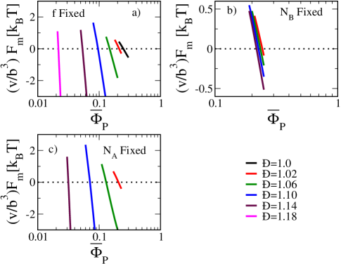
Figure S1: Micelle formation energies $F_{m}$ as a function of bulk polymer volume fraction $\bar{\phi}_{p}$ in polymer systems with (a) $fFixed$, (b) $N_{B}$ Fixed and (c) $N_{A}$ Fixed. $\DJ$ refers to dispersity in the corresponding polydisperse part of the chain (A or B or total).

For a copolymeric system with given $f$ and Đ, spherical micelles are formed in the system for a range of bulk polymer volume fractions $\left(\bar{\Phi}_{p}\right)$. In Figure S1, we report micelle free energies $F_{m}$ of different systems investigated in this work. As noted in the main manuscript, $F_{m}$ is computed as the free energy difference of a system containing a micelle and the corresponding homogeneous bulk system. Irrespective of the system investigated, $F_{m}$ is seen to be a decreasing function of ($\bar{\Phi}_{p}$). For given value of $f$, we fix a slightly positive value of $F_{m}$. Then, for each Đ, we choose that particular $\bar{\Phi}_{P}$ which results in the specified micelle free energy $F_{m}$. The model parameters used in this work are summarized in table S1.

Table S1: Parameters to simulate spherical micelles formed by diblock copolymer micelles. $\DJ$ refers to the dispersity in the corresponding polydisperse part of the chain (A or B or total).

Polymeric system	Micelle free energy	k $\left(\mbox{\DJ}\right)$	$\bar{\Phi}_{p}$
$fFixed$	$F_{m}\approx 3\times 10^{-3}\bar{C}k_{B}T$	5.5 (1.18)	2.16e-02
		7.14 (1.14)	5.35e-02
		10 (1.10)	9.58e-02
		16.6 (1.06)	1.48e-01
		50 (1.02)	2.12e-01
		MD (1.00)	2.47e-01
$N_{B}$ Fixed	$F_{m}\approx 3\times 10^{-3}\bar{C}k_{B}T$	7.14 (1.14)	3.15e-02
		10 (1.10)	7.10e-02
		16.6 (1.06)	1.30e-02
		50 (1.02)	2.06e-02
$N_{A}$ Fixed	$F_{m}\approx 3\times 10^{-3}\bar{C}k_{B}T$	7.14 (1.14)	2.18e-01
		10 (1.10)	2.26e-01
		16.6 (1.06)	2.34e-01
		50 (1.02)	2.43e-01

.3 Energy decomposition

In order to analyze the driving force for the effect of polymer dispersity on the size distribution of micelles, we decomposed micelle free energy $F_{m}$ into the interaction energy ($\Delta U$), the entropy ($T\Delta S$), and the chemical work ($W_{Chem}$). Within self consistent field theory, the entropy and the chemical work can be further decomposed into the corresponding contributions from polymer and solvent components:

$$F_{m} =\Delta U-T\Delta S+W_{Chem}$$

$$=\Delta U-\left(T\Delta S_{P}+T\Delta S_{S}\right)+\left(W_{P}+W_{S}\right)$$ (S8)

In this section, we describe how this decomposition is made. The thermodynamic equation governing grand canonical ensemble is given by

$$\Omega=U-TS-\sum_{Z}\mu_{Z}n_{Z}$$ (S9)

In the above equation, $\Omega$ is the grand potential, $U$ is the internal energy, $S$ is the entropy, $T$ is the temperature, $\mu_{Z}$ is the chemical potential of species $Z$ and $n_{Z}$ is the number of particles of type X in the given system. Note that every copolymer length $X=N/N_{n}$ defines a separate species, hence $Z$ runs over $S$ (solvent) and ($p,X$) (copolymers of length $X$). Comparing the Equation (S9) to the Equation (S1), the following relations can be deduced:

$$\frac{U}{\bar{C}k_{B}T} =\frac{1}{\bar{R}^{3}_{g}}\int{\rm d}^{3}r\left\{\tilde{\chi}_{AB}\phi_{A}\phi_{B}+\tilde{\chi}_{AS}\phi_{A}\phi_{S}+\tilde{\chi}_{BS}\phi_{B}\phi_{S}\right\}$$

$$\qquad+\frac{\tilde{\kappa}_{H}}{2\bar{R}^{3}_{g}}\int{\rm d}^{3}r\left(\phi_{A}+\phi_{B}+\phi_{S}-1\right)^{2}$$ (S10)

$$-\left(TS+\sum_{Z}\mu_{Z}n_{Z}\right)/\left(\bar{C}k_{B}T\right)=-\frac{1}{\bar{R}^{3}_{g}}\int{\rm d}^{3}r\left\{\phi_{A}\tilde{\omega}_{A}+\phi_{B}\tilde{\omega}_{B}+\phi_{S}\tilde{\omega}_{S}\right\}$$

$$-\int dZ\exp\{\mu_{p}\left(X\right)/k_{B}T\}Q_{p}\left(X\right)-\exp\left\{\mu_{S}/k_{B}T\right\}Q_{S}$$ (S11)

Equation (S11) can be readily decomposed into polymer (P) and solvent (S) contributions as follows,

$$-\left(TS+\sum_{Z}\mu_{Z}n_{Z}\right)_{P}/\left(\bar{C}k_{B}T\right) =-\frac{1}{\bar{R}^{3}_{g}}\int{\rm d}^{3}r\left\{\phi_{A}\tilde{\omega}_{A}+\phi_{B}\tilde{\omega}_{B}\right\}$$

$$\qquad-\int dX\exp\{\mu_{p}\left(X\right)/k_{B}T\}Q_{p}\left(X\right)$$ (S12)

$$-\left(TS+\sum_{Z}\mu_{Z}n_{Z}\right)_{S}/\left(\bar{C}k_{B}T\right) =-\frac{1}{\bar{R}^{3}_{g}}\int{\rm d}^{3}r\left\{\phi_{S}\tilde{\omega}_{S}\right\}-\exp\left\{\mu_{S}/k_{B}T\right\}Q_{S}$$ (S13)

Using Equation (S2), the specific contribution of polymer molecules to the chemical work can be computed as

$$W_{P} =-\sum_{X}\mu_{P}\left(X\right)n_{X}$$

$$n_{N} =\frac{1}{X\bar{R}^{3}_{g}}\int{\rm d}^{3}r\left(\phi_{A,X}+\phi_{B,X}\right)$$ (S14)

where $\phi_{A,X}$ and $\phi_{B,X}$ correspond to the rescaled segment densities of type A and B of polymer molecules with $X=N/N_{n}$ segments per chain. Similarly, using Equation (S3), the contribution of solvent particles to the chemical work can be computed as

$$W_{S} =-\mu_{S}n_{S}$$

$$n_{S} =\frac{1}{\bar{R}^{3}_{g}}\int{\rm d}^{3}r\phi_{S}$$ (S15)

Based on this decomposition of chemical work into polymer and solvent contributions, we can write the corresponding entropic contributions as

$$-\left(TS\right)_{P}=-\left(TS+\sum_{Z}\mu_{Z}n_{Z}\right)_{P}-W_{P}$$ (S16)

$$-\left(TS\right)_{S}=-\left(TS+\sum_{Z}\mu_{Z}n_{Z}\right)_{S}-W_{S}$$ (S17)

.4 Additional data

In the following, we first show the data for the chain length distribution in the micelles compared to the bulk ( for the systems with $N_{B}$ Fixed and $N_{A}$ Fixed Fig. S2) then the average length of the solvophobic part of the chain in the micelle for all the three systems investigated in this work (Fig. S3) and then data for the micelle free energies as a function of micelle radius for the systems with $N_{B}$ Fixed and $N_{A}$ Fixed (Fig. S4).

When length of the solvophobic part of the chain is fixed, it is seen that the chain length distribution in the micelle overlaps with that in the bulk ((Fig. S2(right)). In contrast, at higher dispersities, chain length distribution in the micelle deviates from that in the bulk when solvophilic part of the chain is fixed ((Fig. S2(left)). Interestingly, at a given Đ, there are more solvophobic segments in the micelle formed by the system with $N_{B}$ Fixed when compared to that of $f=0.5$ (Fig. S3). Consistent with the above results, we note from Fig. S4, that the effect of polymer chain dispersity on micelle free energy $F_{m}$ is only prominent when the solvophobic part of the chain is polydisperse in nature.

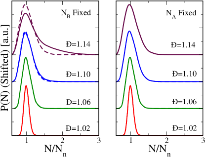
Figure S2: Chain length distribution of copolymers in the bulk (dashed) and in the most probable micelle (solid) for (left) systems with $"N_{B}fixed"$ and (right) for systems with $"N_{A}fixed"$. Here, $\DJ$ refers to dispersity in the corresponding polydisperse part of the chain (A or B)

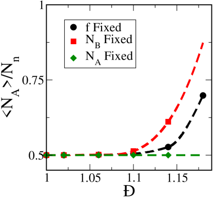
Figure S3: Average length of the solvophobic part of the polymer chain in the micelle for systems with different chain architectures at different values of $\DJ$. Here, $\DJ$ refers to dispersity in the corresponding polydisperse part of the chain (A or B or total)

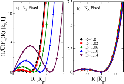
Figure S4: Micelle free energy vs. micelle radius for solvophobic fraction (a) $N_{B}$ Fixed and (b) $N_{A}$ Fixed. Symbols show SCF results, lines a fit to the fourth order polynomial $\sum_{n=1}^{4}a_{n}x^{n}$. $\DJ$ refers to dispersity in the corresponding polydisperse part of the chain (A or B)

References

- Bucaro et al. (2009) M. A. Bucaro, P. Kolodner, J. A. Taylor, A. Sidorenko, J. Aizenberg, and T. N. Krupenkin, Langmuir 25, 3876 (2009).
- Ethirajan and Landfester (2010) A. Ethirajan and K. Landfester, Chemistry 16, 9398 (2010).
- Nasir et al. (2015) A. Nasir, A. Kausar, and A. Younus, Polymer-plastics technology and engineering 54, 325 (2015).
- Ulbrich et al. (2016) K. Ulbrich, K. Holá, V. Šubr, A. Bakandritsos, J. Tuček, and R. Zbořil, Chem. Rev. 116, 5338 (2016).
- Tibbitt et al. (2016) M. W. Tibbitt, J. E. Dahlman, and R. Langer, J. Am. Chem. Soc. 138, 704 (2016).
- Förster and Plantenberg (2002) S. Förster and T. Plantenberg, Angew. Chemie Intnl. Ed. 41, 688 (2002).
- Rodriguez-Hernandez et al. (2005) J. Rodriguez-Hernandez, F. Checot, Y. Gnanou, and S. Lecommandoux, Prog. Polym. Sci. 30, 691 (2005).
- Leermakers et al. (1995) F. A. M. Leermakers, C. M. Wijmans, and G. J. Fleer, Macromolecules 28, 3434 (1995).
- Webber (1998) S. E. Webber, J. Phys. Chem. B 102, 2618 (1998).
- Riess (2003) G. Riess, Prog. Polym. Sci. 28, 1107 (2003).
- Lebouille et al. (2013) J. G. J. L. Lebouille, L. F. W. Vleugels, A. A. Dias, F. A. M. Leermakers, M. A. Cohen Stuart, and R. Tuinier, Eur. Phys. J. E 36, 107 (2013).
- Feng et al. (2014) S.-T. Feng, J. Li, Y. Luo, T. Yin, H. Cai, Y. Wang, Z. Dong, X. Shuai, and Z.-P. Li, PLOS ONE 9, 1 (2014).
- Nakayama and Okano (2006) M. Nakayama and T. Okano, J. Drug Delivery Sci. Technol. 16, 35 (2006).
- Kataoka et al. (2001) K. Kataoka, A. Harada, and Y. Nagasaki, Adv. Drug Delivery Rev. 47, 113 (2001).
- Cabral et al. (2011) H. Cabral, Y. Matsumoto, K. Mizuno, Q. Chen, M. Murakami, M. Kimura, Y. Terada, M. R. Kano, K. Miyazono, M. Uesaka, N. Nishiyama, and K. Kataoka, Nature Nanotechnology 6, 815 (2011).
- Chang et al. (2014) T. Chang, M. S. Lord, B. Bergmann, A. Macmillan, and M. H. Stenzel, J. Mater. Chem. B 2, 2883 (2014).
- Seno et al. (2007) K.-I. Seno, S. Kanaoka, and S. Aoshima, J. Polymer Sci. A 46, 2212 (2007).
- Lynd et al. (2008) N. A. Lynd, A. J. Meuler, and M. A. Hillmyer, Prog. Polym. Sci. 33, 875 (2008).
- Doncom et al. (2017) K. E. B. Doncom, L. D. Blackman, D. B. Wright, M. I. Gibson, and R. K. O’Reilly, Chem. Soc. Rev. 46, 4119 (2017).
- Nelson et al. (1997) P. H. Nelson, G. C. Rutledge, and T. A. Hatton, J. Chem. Phys. 107, 10777 (1997).
- Widin et al. (2012) J. M. Widin, A. K. Schmitt, A. L. Schmitt, K. Im, and M. K. Mahanthappa, J. Am. Chem. Soc. 134, 3834 (2012).
- Qi et al. (2016) S. Qi, L. I. Klushin, A. M. Skvortsov, and F. Schmid, Macromolecules 49, 9655 (2016).
- Romeis and Sommer (2015) D. Romeis and J.-U. Sommer, ACS Appl. Mater. Interfaces 7, 12496 (2015).
- Skvortsov et al. (1997) A. M. Skvortsov, L. I. Klushin, and A. A. Gorbunov, Macromolecules 30, 1818 (1997).
- Merlitz et al. (2008) H. Merlitz, G.-L. He, C.-V. Wu, and J.-U. Sommer, Macromolecules 41, 5070 (2008).
- Romeis and Sommer (2013) D. Romeis and J.-U. Sommer, J. Chem. Phys. 139, 044910 (2013).
- Nguyen et al. (1994) D. Nguyen, X.-F. Zhong, C. E. Williams, and A. Eisenberg, Macromolecules 27, 5173 (1994).
- Matsushita et al. (2003) Y. Matsushita, A. Noro, M. Iinuma, J. Suzuki, H. Ohtani, and A. Takano, Macromolecules 36, 8074 (2003).
- Sides and Fredrickson (2004) S. W. Sides and G. H. Fredrickson, J.Chem.Phys. 121, 4974 (2004).
- Noro et al. (2005) A. Noro, D. Cho, A. Takano, and Y. Matsushita, Macromolecules 38, 4371 (2005).
- Wang et al. (2005) J. Wang, Z.-G. Wang, and Y. Yang, Macromolecules 38, 1979 (2005).
- Ruzette et al. (2006) A.-V. Ruzette, S. Tencé-Girault, L. Leibler, F. Chauvin, D. Bertin, O. Guerret, and P. Gérard, Macromolecules 39, 5804 (2006).
- Torikai et al. (2006) N. Torikai, A. Noro, M. Okuda, F. Odamaki, D. Kawaguchi, A. Takano, and Y. Matsushita, Physica B 385-386, 709 (2006).
- Lynd and Hillmyer (2005) N. A. Lynd and M. A. Hillmyer, Macromolecules 38, 8803 (2005).
- Lynd and Hillmyer (2007) N. A. Lynd and M. A. Hillmyer, Macromolecules 40, 8050 (2007).
- Lynd et al. (2007) N. A. Lynd, B. D. Hamilton, and M. A. Hillmyer, J. Polym. Sci., Part B: Polym. Phys. 45, 3386 (2007).
- Park et al. (2008) S. Park, D. Y. Ryu, J. K. Kim, M. Ree, and T. Chang, Polymer 49, 2170 (2008).
- Matsen (2006) M. W. Matsen, Eur. Phys. J. E 21, 199 (2006).
- Matsen (2007) M. W. Matsen, Phys. Rev. Lett. 99, 148304 (2007).
- Cooke and Shi (2006) D. M. Cooke and A.-C. Shi, Macromolecules 39, 6661 (2006).
- Oschmann et al. (2017) B. Oschmann, J. Lawrence, M. Schulze, J. Ren, A. Anastasak, Y. Luo, M. Nothling, C. Pester, K. Delaney, L. A. Connal, A. J. Mcgrath, P. G. Clark, C. M. Bates, and C. J. Hawker, ACS Macro Lett 6, 668 (2017).
- Gao and Eisenberg (1993) Z. Gao and A. Eisenberg, Macromolecules 26, 7353 (1993).
- Linse (1994) P. Linse, Macromolecules 27, 6404 (1994).
- Khougaz et al. (1994) K. Khougaz, Z. Gao, and A. Eisenberg, Macromolecules 27, 6341 (1994).
- Hvidt et al. (2002) S. Hvidt, C. Trandum, and W. Batsberg, J. Coll. Interf. Sci. 250, 243 (2002).
- Terreau et al. (2003) O. Terreau, L. Luo, and A. Eisenberg, Langmuir 19, 5601 (2003).
- Jiang et al. (2005) Y. Jiang, T. Chen, F. Ye, H. Liang, and A.-C. Shi, Macromolecules 38, 6710 (2005).
- Li et al. (2009) F. Li, S. Prevost, R. Schweins, A. T. M. Marcelis, F. A. M. Leermakers, M. A. Cohen Stuart, and E. J. R. Sudhölter, Soft Matter 5, 4169 (2009).
- Schmitt et al. (2012) A. L. Schmitt, M. H. Repollet-Pedrosa, and M. K. Mahanthappa, ACS Macro Lett. 1, 300 (2012).
- Fredrickson and Sides (2003) G. H. Fredrickson and S. W. Sides, Macromolecules 36, 5415 (2003).
- Doi and Edwards (1986) M. Doi and S. F. Edwards, The Theory of Polymer Dynamics (Oxford University Press, 1986).
- Fredrickson (2006) G. H. Fredrickson, The Equilibrium Theory of Inhomogeneous Polymers (Oxford University Press, 2006).
- He and Schmid (2006) X. He and F. Schmid, Macromolecules 39, 2654 (2006).
- Helfand (1975) E. Helfand, J. Chem. Phys. 62, 999 (1975).
- Schmid (1998) F. Schmid, J. Phys.: Cond. Matter 10, 8105 (1998).
- Schmid (2011) F. Schmid, “Theory and simulation of multiphase polymer systems,” in Handbook of Multiphase Polymer Systems (Wiley-Blackwell, 2011) Chap. 3, pp. 31–80.
- Qi and Yan (2008) S. Qi and D. Yan, J. Chem. Phys. 129, 204902 (2008).
- Glaser et al. (2014) J. Glaser, P. Medapuram, T. M. Beardsley, M. W. Matsen, and D. C. Morse, Phys. Rev. Lett. 113, 068302 (2014).
- Bates et al. (1994) F. S. Bates, M. F. Schulz, A. K. Khandpur, S. Förster, J. H. Rosedale, K. Almdal, and K. Mortensen, Faraday Discuss. 98, 7 (1994).
- Bates et al. (1990) F. S. Bates, J. H. Rosedale, and G. H. Fredrickson, J.Chem.Phys. 92, 6255 (1990).
- Bates et al. (1988) F. S. Bates, J. H. Rosedale, G. H. Fredrickson, and C. J. Glinka, Phys. Rev. Lett. 61, 2229 (1988).
- Wang et al. (2010) J. Wang, K. Guo, L. An, M. Müller, and Z.-G. Wang, Macromolecules 43, 2037 (2010).
- Wang and Wang (2012) R. Wang and Z.-G. Wang, Macromolecules 45, 6266 (2012).
- Bleul et al. (2015) R. Bleul, R. Thiermann, and M. Maskos, Macromolecules 48, 7396 (2015).
- Nikoubashman et al. (2016) A. Nikoubashman, V. E. Lee, C. Sosa, R. K. Prud’homme, R. D. Priestley, and A. Z. Panagiotopoulos, ACS Nano 10, 1425 (2016).
- Kessler et al. (2017) S. Kessler, K. Drese, and F. Schmid, Polymer 126C, 9 (2017).