Interpolating the Schwarzschild and de-Sitter metrics

Abstract

The binary potential technique of interpolation (by M. Riesz, Acta Math. 81, 1 (1949)) is applied to some well-known metrics of general relativity. These include Schwarzschild, de Sitter and 2+1-dimensional BTZ spacetimes. In particular, the Schwarzschild-de Sitter solution is analyzed in some detail with a finite range parameter. Reasoning by the high level of non-linearity and absence of a superposition law necessitates search for alternative approaches. We propose the method of interpolation between different spacetimes as one such possibility paving the way toward controlling the two-metric system by a common parameter.

I Introduction

The renowned Majumdar-Papapetrou solution 1 ; 2 ; 3 ; 4 ; 5 ; 6 describes a multi-black hole solution in which the electromagnetic and gravitational forces balance each other. The black holes are not located arbitrarily but rather they lie on an axis along which the attractive / repulsive force act. Many-body problems, even the two-body, have always been tough in physics and general relativity doesn’t provide an exception in this regard. An important lesson we learned from quantum theory is; particles that were connected / interacted in the past by some mechanism remain ever connected in the future albeit through a spooky action at a distance. This is known as the Einstein-Podolsky-Rosen (EPR) paradox 7 , keeping things entangled through spacetime. Is there an analogue picture in classical relativity where particles are to be replaced by spacetimes? In other words, can we connect / couple two different spacetimes by a continuous parameter such that at one end it yields the first while at the other end the second spacetime? Although mathematically this is the process of interpolating two different solutions it may be considered as a classical analogue of entanglement for the two spacetimes. It was argued R1 (and references cited therein) that the two distant particles may be connected through a spacetime wormhole. A wormhole is a solution to the equations of classical general relativity obeying the chronology protection whereas a spooky connection violates causality. How to reconcile a classical wormhole with a spooky quantum action? Further, unless one resorts to the quantum fluctuations at the Planck scale the wormholes constructed  from Schwarzschild-related black holes are not traversable. Our motivation originated from the fact that within classical theory we must find a way to imitate the non-local effects. We aim to do this by introducing a family of metrics governed by one (or more) control / interpolation parameter. The method may be considered as an alternative to the one of wormhole connection. The examples that we discuss here are the Schwarzschild (S) 8 , Bañados-Teitelboim-Zanelli (BTZ) 9 , and de Sitter 10 ; 11 spacetimes. We note that there have been previous examples that used to interpolate different spacetimes 12 . Let us draw a rough analogy. In a classical two-bit system (say A and B) we are confronted with the simple rule: either A or B with no gray zone. In a quantum system of qubits on the other hand we have infinite possibilities as representation of the gray zone between A and B. The same is expected to hold in a quantum gravity that acts as the covering space to all possible spacetimes. In certain sense this is similar to Feynman’s path integral picture where each path has certain probability. Why is interpolation / entanglement of A and B so important? We recall that wave-particle duality of quantum theory allows states such as 30% particle 70% wave and so on. Through inherent non-linearity general relativity provides an arena in which all sources contribute to the resulting spacetime. The mathematical procedure developed by Riesz 13 covers the simplest two-level systems which have two fixed end states interpolated by a single parameter. Clearly our spacetimes at hand are not at the level of bits or qubits, but the method of classical interpolation bears traces of reminiscences to particle state superposition. It is not difficult to anticipate that as superposition law lies at the heart of quantum theory interpolation of spacetimes may play a similar role in a futuristic quantum gravity. Mathematically we admit that interpolation is not a unique process; different parametrization leads to different gray zone spacetimes.

In this study by resorting to the Riesz potential / interaction approach 13 for two bodies we wish to reinterpret the analogous problems in general relativity. Our aim can be summarized with the following examples.

A) The Coulomb potential is given by $V\left(r\right)=\frac{Q}{r},$ for charge $Q.$ Following Riesz 13 we redefine this potential by

$$V\left(r,s\right)=\frac{1}{s}\left(1-e^{-\frac{Qs}{r}}\right)$$ (1)

for the parameter $0\leq s<\infty.$ Obviously this potential interpolate the Coulomb field ($s\rightarrow 0$) with the vacuum ($s\rightarrow\infty$). Thus (1) acts as a screening potential with the screening parameters for the Coulomb field. (Note that for $Q<0$ we choose $-\infty<s\leq 0.$)

B) The static Schwarzschild (S) metric is given by

$$ds^{2}=-f\left(r\right)dt^{2}+\frac{dr^{2}}{f\left(r\right)}+r^{2}\left(d\theta^{2}+\sin^{2}\theta d\varphi^{2}\right)$$ (2)

with $f\left(r\right)=1-\frac{2m}{r}.$ We modify this line element now by

$$f\left(r,s\right)=1+\frac{1}{s}\left(e^{-\frac{2m}{r}s}-1\right)$$ (3)

where $0\leq s<\infty$ is a constant parameter that interpolates between a S black hole and flat spacetime. Indeed, we have

$$\lim_{s\rightarrow 0}f\left(r,s\right)=1-\frac{2m}{r}$$ (4)

and

$$\lim_{s\rightarrow\infty}f\left(r,s\right)=1.$$ (5)

To have a black hole solution we must choose $0\leq s<1,$ whereas the particular case $s=1$ matches with the S solution in the first order of expansion.

The source created by the parameter $0<s<\infty$ deserves a separate study which is out of our scope in this paper. The parameter $s$ may be interpreted as a screening parameter for the S black hole. For $s>1,$ the solution loses its black hole property, and for $s\gg 1$ we approach to the flat (or vacuum) spacetime.

C) In a similar manner we consider the charged BTZ spacetime with zero angular momentum in $2+1-$dimensions

$$ds^{2}=-g\left(r\right)dt^{2}+\frac{dr^{2}}{g\left(r\right)}+r^{2}d\varphi^{2}$$ (6)

where

$$g\left(r\right)=-M+\left(\frac{r}{\ell}\right)^{2}-\frac{Q^{2}}{2}\ln\left(\frac{r}{r_{0}}\right).$$ (7)

The parameters $M,\ell$ and $Q$ are related to mass, cosmological constant and electric charge, respectively, while $r_{0}$ is a scaling constant (with $r>r_{0}$).

As in the S case (B) above, and following the Riesz potential approach we revise the BTZ spacetime metric function accordingly as

$$g\left(r,s,p\right)=-M+\frac{1}{s}\left(1-e^{-s\left(\frac{r}{\ell}\right)^{2}}\right)+\frac{Q^{2}}{2p}\left(\left(\frac{r_{0}}{r}\right)^{p}-1\right).$$ (8)

Here $0\leq s,p<\infty$ are parameters that interpolate between the vacuum ($s,p\rightarrow\infty$)  by fixing the constant $M,$ and charged BTZ ($s,p\rightarrow 0$) spacetime. Obviously for $Q=0,$ $s$ interpolates the vacuum with the cosmological constant spacetime. It is seen that charged BTZ metric provides an example of two parametric interpolation in accordance with the Riesz’s prescription.

Along similar line of thought, but excluding the flat space as a limit we consider two basic spacetimes such as S and dS and interpolate them by a parameter as described in the next section.

II Schwarzschild-de Sitter spacetime

For many reasons the Schwarzschild (S) and de-Sitter (dS) spacetimes are two best known / cited exact solutions in general relativity. The first (S) is a black hole solution while the second (dS) is a cosmological solution. The intersection / coexistence of the two is known as the Schwarzschild- de Sitter (SdS) solution. To understand non-rotating black holes in cosmology, their thermodynamics, particle creation etc. this solution provides a basic reference (see for instance 14 ). Being so important it deserves to revisit such a spacetime from a different perspective.

Our line element is chosen now to be

$$ds^{2}=-f\left(r\right)dt^{2}+\frac{dr^{2}}{f\left(r\right)}+r^{2}\left(d\theta^{2}+\sin^{2}\theta d\varphi^{2}\right)$$ (9)

where

$$f\left(r\right)=1-2\frac{M_{0}}{r}\sin\lambda-\left(\frac{r}{\ell_{0}}\right)^{2}\cos\lambda$$ (10)

in which $0\leq\lambda\leq\frac{\pi}{2}$ is the interpolation parameter. Obviously by a redefinition

$$M=M_{0}\sin\lambda$$ (11)

and

$$\frac{1}{\ell^{2}}=\frac{1}{\ell_{0}^{2}}\cos\lambda$$ (12)

we have the standard SdS metric satisfying the constraint condition

$$\left(\frac{M}{M_{0}}\right)^{2}+\left(\frac{\ell_{0}}{\ell}\right)^{4}=1.$$ (13)

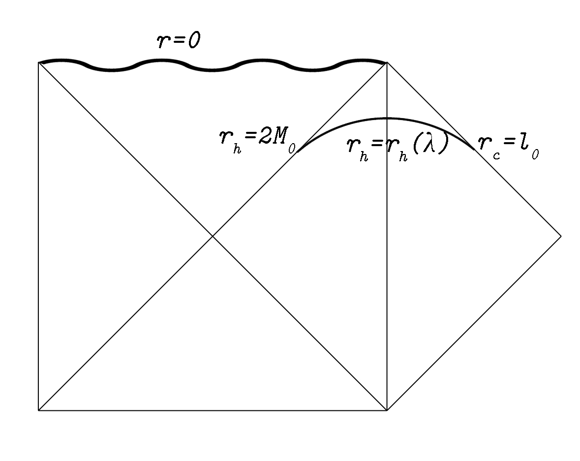
Figure 1: Penrose diagram for the SdS spacetime. The black hole horizon $r_{h}=2M_{0}$ and the cosmological horizon $r_{c}=\ell_{0}$ are interpolated by the curve $r_{h}\left(\lambda\right).$ The particular case $r_{h}=r_{c},$ which amounts to $\frac{M_{0}}{\ell_{0}}\sin\lambda\sqrt{\cos\lambda}=\frac{1}{3\sqrt{3}},$ corresponds to the Nariai limit. Detailed plots are given in the following figures.

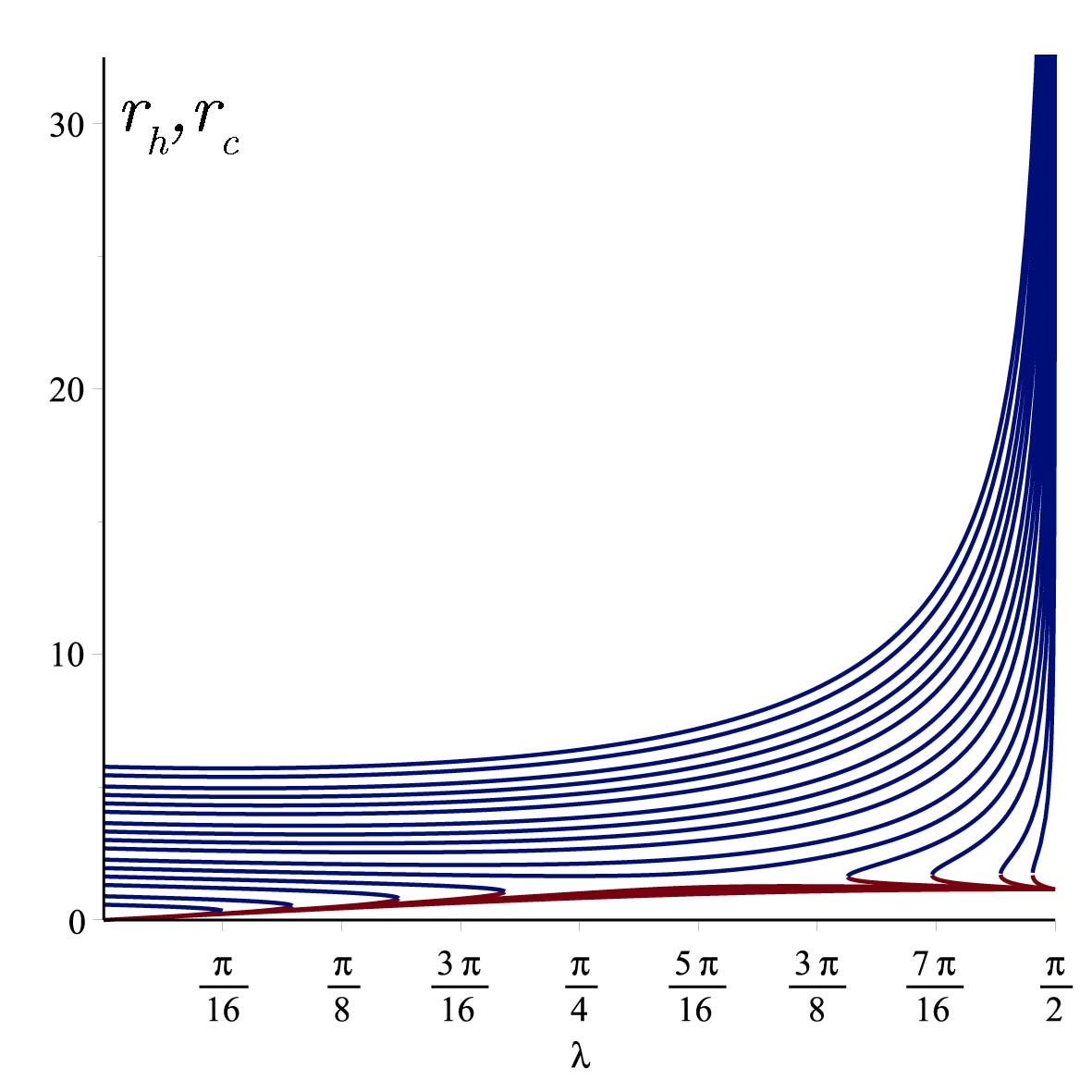
Figure 2: $r_{h}$ (red) and $r_{c}$ (blue) versus $\lambda$ for various $1\leq\ell_{0}\leq 10$ with $\Delta\ell_{0}=0.2.$ At $\ell_{0}=3.224$ the horizons coincide.

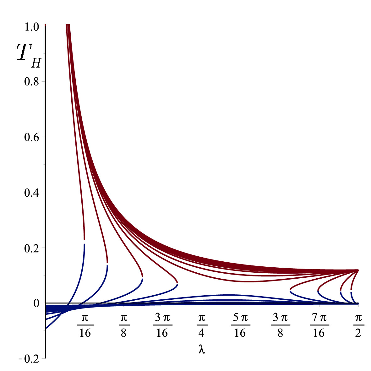
Figure 3: $T_{H}$ at $r_{h}$ (red) and $r_{c}$ (blue) versus $\lambda$ for various $1\leq\ell_{0}\leq 10$ with $\Delta\ell_{0}=0.2.$ At $\ell_{0}=3.224$ the two temperatures coincide.

In the original SdS metric the parameters $M_{0}$ and $\ell_{0}$ are independent parameters coupled through the non-linear dynamics of general relativity. We go one more step forward to entangle / couple them through the parameter $\lambda.$ The interpolation parameter $\lambda$ can appropriately be dubbed also as a mixing angle between $M_{0}$ and $\ell_{0}.$ It can be interpreted through (11) that $\ell_{0}$ makes / dresses the mass: the local mass $M_{0}$ is coupled with the cosmological $\ell_{0},$ as implied by the Mach Principle. Stated otherwise, at each point of spacetime we have a cosmologically induced mass. Upon this arrangement the entire dynamics of the SdS spacetime becomes dependent on the parameter $\lambda.$ For each choice of $0<\lambda<\frac{\pi}{2}$ we have a spacetime with entangled $M$ and $\ell$ through (11) and (12). The Penrose diagram for the SdS spacetime is shown in Fig. 1. Einstein’s equations are summarized as

$$G_{\mu}^{\nu}=R_{\mu}^{\nu}-\frac{1}{2}R\delta_{\mu}^{\nu}=T_{\mu}^{\nu}$$ (14)

where

$$T_{\mu}^{\nu}=\left(\rho+p\right)u_{\mu}u^{\nu}+p\delta_{\mu}^{\nu}$$ (15)

so that with the choice $u^{\mu}=\delta_{0}^{\mu},$

$$\rho=\frac{3\cos\lambda}{\ell_{0}^{2}}>0$$ (16)

and

$$p=-\frac{3\cos\lambda}{\ell_{0}^{2}}<0$$ (17)

and the energy condition

$$\rho+p=0$$ (18)

holds. The fact that $\rho>0$ justifies our choice of the interpolation parameter in the interval $0<\lambda<\frac{\pi}{2}.$ Accordingly the scalar curvature is

$$R=\frac{12\cos\lambda}{\ell_{0}^{2}}$$ (19)

and the Kretschmann scalar becomes

$$K=24\left(\frac{\cos^{2}\lambda}{\ell_{0}^{2}}+\frac{2M_{0}^{2}\sin^{2}\lambda}{r^{6}}\right).$$ (20)

All the physical properties of SdS spacetime are also interpolated. The double horizons i.e., event and cosmological for instance, from $f\left(r\right)=0,$ yields

$$r_{h}=\frac{2\ell_{0}}{\sqrt{3}\cos\lambda}\cos\left(\frac{\psi+\pi}{3}\right)$$ (21)

and

$$r_{c}=\frac{2\ell_{0}}{\sqrt{3}\cos\lambda}\cos\left(\frac{\psi-\pi}{3}\right)$$ (22)

in which

$$\cos\psi=3\sqrt{3}\left(\frac{M_{0}}{\ell_{0}}\right)\sin\lambda\sqrt{\cos\lambda}.$$ (23)

Fig. 2 plots the graphs of $r_{h}$ and $r_{c}$ in terms of $\lambda$ and various values of $\ell_{0}.$We recall that $r_{h}$ and $r_{c}$ are the black hole and cosmological horizons, respectively. In other words, it can be checked that for $\lambda\rightarrow 0$ we get $r_{c}=\ell_{0},$ and for $\lambda\rightarrow\frac{\pi}{2}$ it yields $r_{h}=2M_{0}$, as it should. Let us note that for real roots we impose the condition

$$\left(\frac{M_{0}}{\ell_{0}}\right)^{2}\cos\lambda\sin^{2}\lambda\leq\frac{1}{27}.$$ (24)

For the case $\psi=0,$ the two horizons coincide (i.e., $r_{h}=r_{c}=\frac{\ell_{0}}{\sqrt{3}\cos\lambda}$) at the Nariai horizon 15 ; 16 . Naturally it has to be imposed also that $\ell_{0}>2M_{0}$. The Hawking temperatures at $r_{h}$ and $r_{c}$ are given respectively by

$$T_{H}=\frac{1}{2\pi}\left|\frac{M_{0}\sin\lambda}{r_{h}^{2}}-\frac{r_{h}\cos\lambda}{\ell_{0}^{2}}\right|$$ (25)

and

$$T_{H}=\frac{1}{2\pi}\left|\frac{M_{0}\sin\lambda}{r_{c}^{2}}-\frac{r_{c}\cos\lambda}{\ell_{0}^{2}}\right|$$ (26)

which are depicted in Fig. 3.

III Conclusion

Schwarzschild (S) and de Sitter (dS) spacetimes are interpolated / connected by the finite parameter $0<\lambda<\frac{\pi}{2}$, which constrains the sources of both spacetimes. The coupling automatically rules the two spacetimes by the common parameter $\lambda.$ Accordingly the horizons, Hawking temperatures and other physical properties are not independent any more, but interpolated as well. Through interpolation the effect of cosmological constant at large is coupled and felt at small with mass and vice versa. In certain sense the two spacetimes become ever coupled in reminiscence with the particle entanglement encountered in quantum theory. With the example of SdS the infinite ($0\leq s<\infty$) range interpolation of Riesz is extended to a finite range. The example of BTZ suggests that each physical parameter is interpolated independently, i.e., with two parameters $s$ and $p.$ The same rule applies also to Reissner-Nordström space and vacuum. As stated above the infinite range parameter of Riesz has been extended to a finite range, and also to the case of more than one parameter. In brief, we propose the interpolation method of two spacetimes, (or in case of two particles) as an alternative to the connection through a wormhole. We add finally that the scope of the technique is not limited by these examples. Given that the process of interpolation is non-unique it can be enriched easily with further applications.

References

- (1) S. D. Majumdar, Phys. Rev. 72, 390 (1947).
- (2) A. Papapetrou, Proc. R. Ir. Acad., A Math. Phys. Sci. A51, 191 (1947).
- (3) J. B. Hartle and S. W. Hawking, Commun. Math. Phys. 26, 87 (1972).
- (4) M. Halilsoy, J. Math. Phys. 34, 3553 (1993).
- (5) M. Halilsoy, Gen. Rel. Grav. 25, 275 (1992).
- (6) S. H. Mazharimousavi and M. Halilsoy, Turkish J. Phys. 40, 163 (2016).
- (7) A. Einstein, B. Podolsky, and N. Rosen, Phys. Rev. 47, 777 (1935).
- (8) N. Bao, J. Pollack and G. N. Remmen, JHEP 1511, 126 (2015).
- (9) K. Schwarzschild, Sitzungsberichte der Königlich Preussischen Akademie der Wissenschaften. 7, 189 (1916).
- (10) M. Bañados, C. Teitelboim and J. Zanelli, Phys. Rev. Lett. 69, 1849 (1992).
- (11) W. de Sitter, Proc. Kon. Ned. Acad. Wet., 19, 1217 (1917).
- (12) W. de Sitter, Proc. Kon. Ned. Acad. Wet., 20, 229 (1917).
- (13) M. Halilsoy and S. H. Mazharimousavi, Phys. Rev. D 88, 064021 (2013).
- (14) M. Riesz, Acta Mathematica, 81, 1 (1949).
- (15) S. Shankaranarayanan, Phys. Rev. D 67, 084026 (2003).
- (16) V. Cardoso, Ó. J. C. Dias and J. P. S. Lemos, Phys. Rev. D 70, 024002 (2004).
- (17) H. Nariai, Sci. Rep. Tohoku Univ., Ser. 1 34, 160 (1950); 35, 62 (1951).