Fukaya’s conjecture on $S^{1}$-equivariant de Rham complex

Abstract.

Getzler-Jones-Petrack [7] introduced $A_{\infty}$ structures on the equivariant complex for manifold $M$ with smooth $\mathbb{S}^{1}$ action, motivated by geometry of loop spaces. Applying Witten’s deformation by Morse functions followed by homological perturbation we obtained a new set of $A_{\infty}$ structures. We extend and prove Fukaya’s conjecture [6] relating this Witten’s deformed equivariant de Rham complexes, to a new Morse theoretical $A_{\infty}$ complexes defined by counting gradient trees with jumping which are closely related to the $\mathbb{S}^{1}$ equivariant symplectic cohomology proposed by Siedel [15].

1. Introduction

In the influential paper [17] by Witten, harmonic forms on a compact oriented Riemannian manifold $(M,g)$ are related to the Morse complex $CM^{*}_{f}:=\bigoplus_{p\in\text{Crit}(f)}\mathbb{C}\cdot p$ on $M$ with a Morse function $f$ . More precisely, Witten introduced the twisted Laplacian $\Delta_{f,\lambda}:=d^{*}_{f,\lambda}\circ d+d\circ d^{*}_{f,\lambda}$ with a large real parameter $\lambda$, and an isomorphism

(1.1) $$\phi:(CM^{*}_{f},\delta)\rightarrow(\Omega^{*}_{f,<1}(M),d)$$

where $\Omega^{*}_{f,<1}(M)$ refers to the small eigensubspace of $\Delta_{f,\lambda}$ (see Section 2.2). The detailed analysis of $\phi$ is later carried out in [9, 11, 10, 12] and readers may also see [18] for this correspondence.

In [6], Fukaya conjectured that Witten’s isomorphism (1.1) can be enhanced to an isomorphism of $A_{\infty}$ algebras (or categories), a generalization of differential graded algebras (abbrev. dga), encoding rational homotopy type by work of Quillen [14] and Sullivan [16]. The $A_{\infty}$ structures $m_{k}(\lambda)$’s on $\Omega^{*}_{f,<1}(M)$ are obtained by pulling back the structures of the de Rham dga $(\Omega^{*}(M),d,\wedge)$ using the homological perturbation lemma (see e.g. [13]) with homotopy operator $H_{f,\lambda}=d^{*}_{f,\lambda}G_{f,\lambda}$. The Morse $A_{\infty}$ structures $m_{k}^{Morse}$’s are defined via counting gradient flow trees of Morse functions as in [5]. Fukaya conjectured that they are related by

(1.2) $$\lim_{\lambda\rightarrow\infty}m_{k}(\lambda)=m_{k}^{Morse}$$

via the Witten’s isomorphism (1.1). This conjectured is proven in [3] by extending the analytic technique in [12] to incorporate the homotopy operator $H_{f,\lambda}$.

When $M$ is equipped with a smooth $\mathbb{S}^{1}$ action, motivated by the geometry of loop space $\mathbb{S}^{1}\curvearrowright\mathscr{L}X$ for some $X$, Getzler-Jones-Petrack [7] introduced an enhancement of the equivariant de Rham complex on $M$. They defined new $A_{\infty}$ algebra structures consisting of

(1.3) $$\tilde{m}_{k}:\big{(}\Omega^{*}(M)[[u]]\big{)}^{\otimes k}\rightarrow\Omega^{*}(M)[[u]]$$

by adding higher order (in $u$) operations $u\mathcal{P}_{k}$’s (see Section 2.1) to ordinary de Rham dga structures. Witten’s deformed $A_{\infty}$ structures $m_{k}(\lambda)$’s are constructed from $\tilde{m}_{k}$’s in (1.3) using the technique of homological perturbation as in original Fukaya’s conjecture.

Inspired by Fukaya’s correspondence, we define new Morse theoretic type counting structures $m_{k}^{\text{eMorse}}$’s (where $m_{1}^{\text{eMorse}}$ is known before in [2]) associated to $\mathbb{S}^{1}\curvearrowright M$, counting of Morse flow trees with jumpings coming from the $\mathbb{S}^{1}$ action (see the following Section 1.1). We prove the generalization of (1.2) for $\mathbb{S}^{1}\curvearrowright M$ relating these two structures.

Theorem 1.1 (=Theorem 2.11).

We have

$$\lim_{\lambda\rightarrow\infty}m_{k}(\lambda)=m_{k}^{\text{eMorse}}.$$

1.1. The operation $m_{k}^{\text{eMorse}}$’s

To describe $m_{k}^{\text{eMorse}}$’s, we fix a generic sequence (see Definition 2.8) of functions $(f_{0},\dots,f_{k})$ such that their differences $f_{ij}:=f_{j}-f_{i}$ are assumed to be Morse-Smale as in Definition 2.5. The Morse theoretical $A_{\infty}$ product $m_{k}^{\text{eMorse}}$’s take the form

$$m_{k}^{\text{eMorse}}:=\sum_{T}m_{k,T}^{\text{eMorse}}:CM^{*}_{f_{(k-1)k}}[[u]]\otimes\cdots\otimes CM^{*}_{f_{01}}[[u]]\rightarrow CM^{*}_{f_{0k}}[[u]]$$

which is a summation over directed labeled ribbon $k$-tree $T$ with $k$-incoming edges and $1$ outgoing edge, where internal vertices are either labeled by $1$ or by $u$. For example (see Section 2.3 for details), if we take the tree $T$ to be the one with two incoming edges $e_{12}$ and $e_{01}$ joining the vertex $v_{r}$ connected to the outgoing edge $e_{02}$, with $v_{r}$ being labeled by $u$. The gradient flow trees with type $T$ will be consisting of gradient flow lines of $f_{12}$, $f_{01}$ and $f_{02}$ which ending at critical points $q_{12}$, $q_{01}$ and $q_{02}$ respectively, that can be joined together at a point $x_{v_{r}}\in M$ with further help of the $\mathbb{S}^{1}$ action $\sigma_{t}:M\rightarrow M$ (for some $t$) as shown in the Figure 1. As a consequence of the above Theorem 1.1, the Morse (pre)-category (here pre-category means this operation only defined for generic sequence $(f_{0},\dots,f_{k})$) on $\mathbb{S}^{1}\curvearrowright M$ is an $A_{\infty}$ (pre)-category.

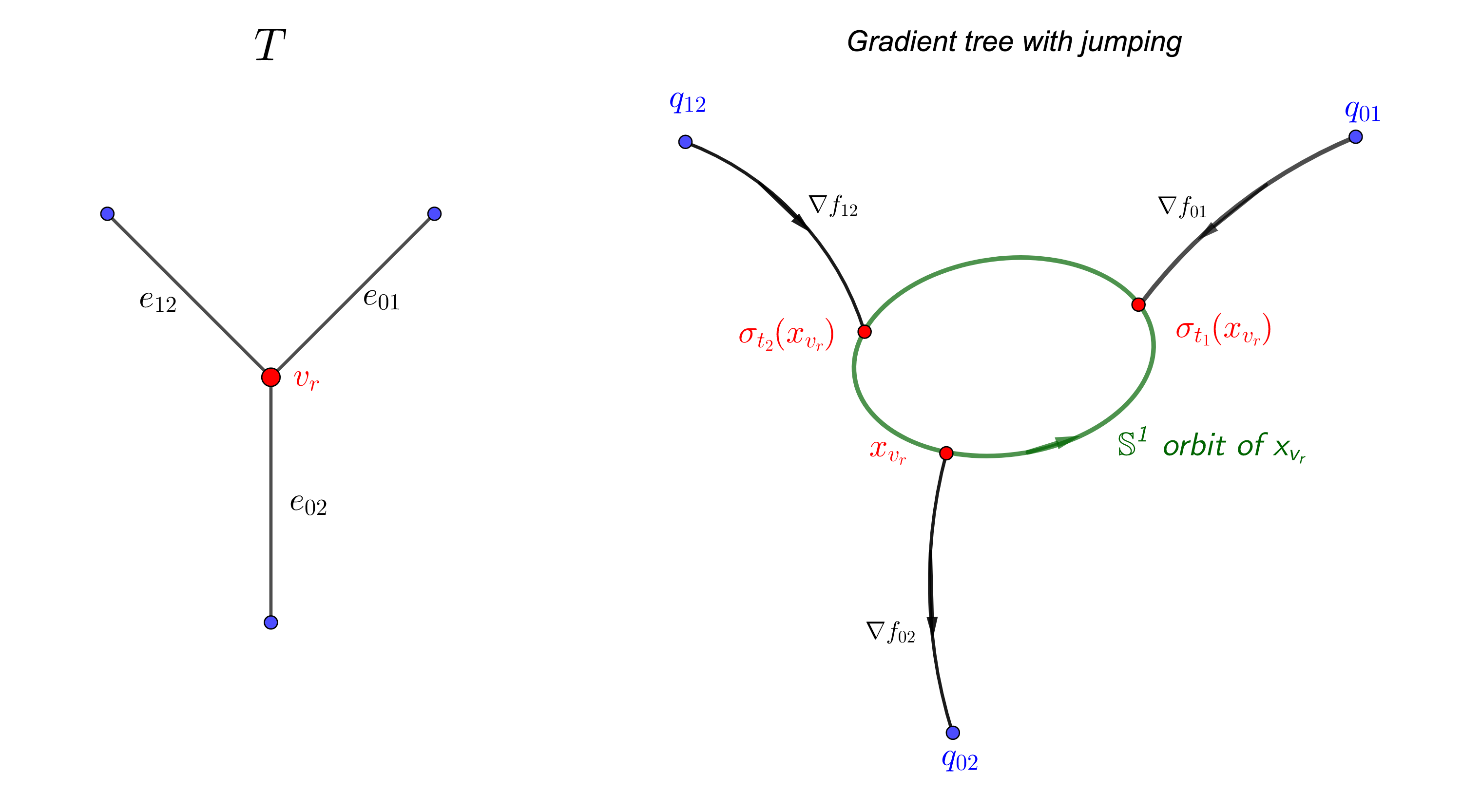
Figure 1. Gradient tree with jumping of type $T$

Corollary 1.2.

The operations $m_{k}^{\text{eMorse}}$’s satisfy the $A_{\infty}$ relation for generic sequences of functions.

Remark 1.3.

In [15, Section 8b], Seidel proposed the $A_{\infty}$ operators $m_{k}^{\text{Floer}}$ on the symplectic cochain complex for a Liouville domain $X$, which corresponds to $m_{k}^{\text{eMorse}}$’s if we think of $M$ as a finite dimensional analogue of $\mathcal{L}X$. The corresponding $m_{1}^{\text{Floer}}$ operation is studied in details in [19]. The above Theorem 1.1 suggest how Witten deformation can provide a linkage between the Getzler-Jones-Petrack’s operation $\tilde{m}_{k}$ on $\mathcal{L}X$ and the Floer theoretical operations introduced by Seidel through the investigation of the corresponding finite dimensional situation.

This paper consists of three parts. In Section 2 we set up the Witten deformation of Getzler-Jones-Petrack’s $A_{\infty}$ operations $\tilde{m}_{k}$’s, the definition of counting gradient flow trees with jumping, and state our Main Theorem 2.11. In Section 3.1, we recall the necessary analytic result by following [3]. The rest of Section 3 will be a proof of Theorem 2.11 by figuring out the exact relations between the operations $m_{k,T}(\lambda)$ and counting of gradient trees.

2. Witten’s deformation of $S^{1}$-equivariant de Rham complex

We always let $(M,g)$ to be an $n$-dimensional compact oriented Riemannian manifold, and denote it volume form by $\operatorname{vol}_{M}$ (or simply $\operatorname{vol}$). We assume there is an smooth $\mathbb{S}^{1}$ action $\sigma:\mathbb{S}^{1}\times M\rightarrow M$ on $M$ preserving $(g,\operatorname{vol})$. We should write $\sigma_{t}:M\rightarrow M$ to be the action for a fixed $t\in\mathbb{S}^{1}$.

2.1. $S^{1}$-equivariant de Rham complex and category

We begin with recalling the Definition of $S^{1}$-equivariant de Rham $A_{\infty}$ algebra introduced in [7], which is reformulated to be $A_{\infty}$ category as follows for the convenient of presentation of this paper.

Definition 2.1.

The $S^{1}$-equivariant de Rham $A_{\infty}$ category $\text{dR}(M)$ consisting of object being smooth functions $f:M\rightarrow\real$, with morphism $\operatorname{Hom}(f,g):=\Omega^{*}(M)[[u]]$ where $u$ is a formal variable. The $A_{\infty}$ operations $\tilde{m}_{k}:\operatorname{Hom}(f_{k-1},f_{k})\otimes\cdots\otimes\operatorname{Hom}(f_{0},f_{1})\cong(\Omega^{*}(M)[[u]])^{\otimes k}\rightarrow\operatorname{Hom}(f_{0},f_{k})\cong\Omega^{*}(M)[[u]]$ is defined by $\tilde{m}_{1}(\alpha_{01})=d(\alpha_{01})+u\mathcal{P}_{1}(\alpha_{01})$, $\tilde{m}_{2}(\alpha_{12},\alpha_{01})=(-1)^{|\alpha_{12}|+1}\alpha_{12}\wedge\alpha_{01}+u\mathcal{P}_{2}(\alpha_{12},\alpha_{01})$ and $\tilde{m}_{k}(\alpha_{(k-1)k},\dots,\alpha_{01})=u\mathcal{P}_{k}(\alpha_{(k-1)k},\dots,\alpha_{01})$ for $\alpha_{ij}\in\operatorname{Hom}(f_{i},f_{j})$.

Here the operator $\mathcal{P}_{k}$ is defined by the action $\mathcal{P}_{1}(\alpha_{ij})=\int_{\mathbb{S}^{1}}(\iota_{\frac{\partial}{\partial t}}\sigma^{*}(\alpha_{ij}))dt$, and for $k\geq 2$ we use

$$\mathcal{P}_{k}(\alpha_{(k-1)k},\dots,\alpha_{01}):=\int_{0\leq t_{k}\leq\cdots\leq t_{1}\leq 1}\left(\iota_{\frac{\partial}{\partial t_{k}}}(\sigma^{*}(\alpha_{(k-1)k}))\wedge\cdots\wedge\iota_{\frac{\partial}{\partial t_{1}}}(\sigma^{*}(\alpha_{01}))\right)dt_{k}\cdots dt_{1}.$$

The fact that the about operations $\tilde{m}_{k}$’s form an $A_{\infty}$ category is proven in [7, Theorem 1.7].

2.2. Homological perturbation via Witten’s deformation

We follow [3, Section 2.2.] to introduced the Witten deformation with a real parameter $\lambda>0$, which is orignated from [17]. For each $f_{i}$ and $f_{j}$, we twist the volume form $\operatorname{vol}$ by $f_{ij}:=f_{j}-f_{i}$ as $\operatorname{vol}_{ij}=e^{-2\lambda f_{ij}}\operatorname{vol}$, and let $d_{ij}^{*}:=e^{2\lambda f_{ij}}d^{*}e^{-2\lambda f_{ij}}=d^{*}+2\lambda\iota_{\nabla f_{ij}}$ to be the adjoint of $d$ with respect to the volume form $\operatorname{vol}_{ij}$. The Witten Laplacian is defined by $\Delta_{ij}:=dd^{*}_{ij}+d^{*}_{ij}d,$ acting on the complex $\Omega^{*}(M)[[u]]$ . We denote the span of eigenspaces with eigenvalues contained in $[0,1)$ by $\Omega^{*}_{ij,<1}(M)[[u]]$, or simply $\Omega^{*}_{ij,<1}[[u]]$. We use construction in [3] originated from [6] using homological perturbation lemma [13], which obtain a new $A_{\infty}$ structure from $m_{k}$’s as follows.

Definition 2.2.

A (directed) $k$-tree labeled $T$ consists of a finite set of vertices $\bar{T}^{[0]}$ together with a decomposition $\bar{T}^{[0]}=T^{[0]}_{in}\sqcup T^{[0]}\sqcup\{v_{o}\},$ where $T^{[0]}_{in}$, called the set of incoming vertices, is a set of size $k$ and $v_{o}$ is called the outgoing vertex (we also write $T^{[0]}_{\infty}:=T^{[0]}_{in}\sqcup\{v_{o}\}$ and $T^{[0]}_{ni}:=T^{[0]}\cup\{v_{o}\}$), a finite set of edges $\bar{T}^{[1]}$, two boundary maps $\partial_{in},\partial_{o}:\bar{T}^{[1]}\rightarrow\bar{T}^{[0]}$ (here $\partial_{in}$ stands for incoming and $\partial_{o}$ stands for outgoing), and a labeling of every internal vertices $T^{[0]}$ by either $1$ or $u$, satisfying the following conditions:

1. Every vertex $v\in T^{[0]}_{in}$ has valency one, and satisfies $\#\partial_{o}^{-1}(v)=0$ and $\#\partial_{in}^{-1}(v)=1$; we let $T^{[1]}:=\bar{T}^{[1]}\setminus\partial_{in}^{-1}(T^{[0]}_{in})$.

2. Every vertex $v\in T^{[0]}$ has an unique edge $e_{v,o}\in\bar{T}^{[1]}$ such that $\partial_{in}(e_{v,o})=v$, and only trivalent vertices in $T^{[0]}$ can be labeled with $1$.

3. For the outgoing vertex $v_{o}$, we have $\#\partial_{o}^{-1}(v_{o})=1$ and $\#\partial_{in}^{-1}(v_{o})=0$; we let $e_{o}:=\partial_{o}^{-1}(v_{o})$ be the outgoing edge and denote by $v_{r}\in T^{[0]}_{in}\sqcup T^{[0]}$ the unique vertex (which we call the root vertex) with $e_{o}=\partial^{-1}_{in}(v_{r})$.

4. The topological realization $|\bar{T}|:=\left(\coprod_{e\in\bar{T}^{[1]}}[0,1]\right)/\sim$ of the tree $T$ is connected and simply connected; here $\sim$ is the equivalence relation defined by identifying boundary points of edges if their images in $T^{[0]}$ are the same.

By convention we also allow the unique labeled $1$-tree with $T^{[0]}=\emptyset$. Two labeled $k$-trees $T_{1}$ and $T_{2}$ are isomorphic if there are bijections $\bar{T}^{[0]}_{1}\cong\bar{T}^{[0]}_{2}$ and $\bar{T}^{[1]}_{1}\cong\bar{T}^{[1]}_{2}$ preserving the decomposition $\bar{T}^{[0]}_{i}=T^{[0]}_{i,in}\sqcup T^{[0]}_{i}\sqcup\{v_{i,o}\}$ and boundary maps $\partial_{i,in}$ and $\partial_{i,o}$ and the labelling of $T^{[0]}$. The set of isomorphism classes of labeled $k$-trees will be denoted by $\mathbb{T}_{k}$. For a labeled $k$-tree $T$, we will abuse notations and use $T$ (instead of $[T]$) to denote its isomorphism class.

A labeled ribbon $k$-tree is a $k$-tree $T$ with a cyclic ordering of $\partial_{in}^{-1}(v)\sqcup\partial_{o}^{-1}(v)$ for each trivalent vertex $v\in T^{[0]}$, and isomorphism of labeled ribbon $k$-trees are further required to preserve this ordering. A labeled ribbon $k$-tree can have its topological realization $|\bar{T}|$ being embedded into the unit disc $D$, with $T^{[0]}_{\infty}$ lying on the boundary $\partial D$ such that the cyclic ordering of $\partial_{in}^{-1}(v)\sqcup\partial_{o}^{-1}(v)$ agree with the anti-clockwise orientation of $D$. The set of isomorphism classes of labeled ribbon $k$-trees will be denoted by $\mathbb{L}\mathbb{T}_{k}$.

Notations 2.3.

For each $T\in\mathbb{L}\mathbb{T}_{k}$, we can associated to each edge $e\in\bar{T}^{[1]}$ a numbering by pair of integer $ij$ using the embedding $|\bar{T}|\rightarrow D$ by the rules: there are $k+1$ connected components of $D\setminus|\bar{T}|$, and we assign each component by integers $0,\dots,k$; each (directed) edge $e\in\bar{T}^{[1]}$ with region numbered by $i$ on its left and region numbered by $j$ on its right is numbered by $ij$; the incoming edges numbered by $e_{(k-1)k},\dots,e_{01}$ and the outgoing edge $e_{0k}$ are in clockwise ordering of $\partial D$.

A pair of $v\in T^{[0]}\cup\{v_{o}\}$ attached to an edge $e\in\bar{T}^{[1]}$ is called a flag, and we will let $\digamma(T)$ to be the set of all flags. For every flag $(e,v)$, we let $T_{e,v}$ to be the unique subtree with outgoing vertex being $v$ if $\partial_{o}(e)=v$, and we let $T_{e,v}$ to be the unique subtree with outgoing edge being $e$ if $\partial_{in}(e)=v$.

Definition 2.4.

Given a labeled ribbon $k$-tree $T\in\mathbb{L}\mathbb{T}_{k}$ with an embedding $|\bar{T}|\rightarrow D$, we assoicate to it an operation $m_{k,T}(\lambda):\Omega^{*}_{(k-1)k,<1}[[u]]\otimes\cdots\otimes\Omega^{*}_{01,<1}[[u]]\rightarrow\Omega^{*}_{0k,<1}[[u]]$ by the following rules :

1. aligning the inputs $\varphi_{(k-1)k},\cdots,\varphi_{01}$ at the incoming vertices $T^{[0]}_{in}$ according to the clockwise ordering induced from $D$;

2. if a vertex $v\in T^{[0]}$ has incoming edges $e_{v,1},\dots,e_{v,l}$ and outgoing edge $e_{v,o}$ attached to it such that $e_{v,l},\dots,e_{v,1},e_{v,o}$ is in clockwise orientation, we apply the operation $\wedge$ if $v$ is labeled with $1$ (and hence trivalent) and the operation $\mathcal{P}_{l}$ if $v$ is labeled with $u$;

3. for an edge $e\in T^{[0]}$ which is numbered by $ij$, we apply the homotopy operator $H_{ij}:=d^{*}_{ij}G_{ij}$ where $G_{ij}$ is the Witten’s twisted Green operator associated to the Witten Laplacian $\Delta_{ij}$;

4. for the unique outgoing edge $e_{o}$, we apply the operator $P_{0k}$ which is the orthogonal projection $P_{0k}:\Omega^{*}[[u]]\rightarrow\Omega^{*}_{0k,<1}[[u]]$ with respect to the twisted $L_{2}$-norm obtained from the volume form $\operatorname{vol}_{0k}$.

By convention, we define $m_{1,T}(\lambda)$ for the unique tree with $T^{[0]}=\emptyset$ to be the restriction of $d$ on $\Omega^{*}_{ij,<1}[[u]]$. For each labeled ribbon $k$-tree $T$, we assign $n_{T}$ to be the number of vertices in $T^{[0]}$ labeled with $u$, and we let $m_{k}(\lambda):=\sum_{T\in\mathbb{L}\mathbb{T}_{k}}u^{n_{T}}m_{k,T}(\lambda)$ to be the homological perturbed $A_{\infty}$ strucutre.

It is well-known that (see e.g. [1, Chapter 8]) the perturbed $A_{\infty}$ structure $m_{k}(\lambda)$’s satisfy the $A_{\infty}$ relation. And we obtain a new category $\text{dR}_{<1}(M)$ via Witten deformation.

2.3. Relation with $S^{1}$-equivariant Morse flow trees

In [12, 17, 18], a relation between the Morse complex $\text{CM}_{f_{ij}}$ and $\Omega^{*}_{ij,<1}$ is established when $f_{ij}$ is a Morse-Smale function in following Definition 2.5. Following [18], it is an isomorphism

(2.1) $$\Phi_{ij}:\Omega^{*}_{ij,<1}\rightarrow\text{CM}_{f_{ij}};\quad\Phi_{ij}(\alpha):=\sum_{p\in\text{Crit}(f_{ij})}\int_{V_{p}^{-}}\alpha,$$

where $\text{Crit}(f_{ij})$ is the finite set of critical points of $f_{ij}$ (with Morse index of $p$ given by number of negative eigenvalues of $\nabla^{2}f_{ij}(p)$), and $V_{p}^{-}$ (Notice that we further choose an orientation of $V_{p}^{-}$ by choosing a volume element of the normal bundle $NV_{p}^{+}$) is the unstable submanifold associated to $p$ which is the union of all gradient flow lines $\gamma(s)$ of $\nabla f_{ij}$ which limit toward $p$ as $s\rightarrow\infty$. Furthermore, the de Rham differential is identified with the Morse differential $\delta_{1}$ defined via counting Morse flow lines.

Definition 2.5.

A Morse function $f_{ij}$ is said to satisfy the Morse-Smale condition if $V^{+}_{p}$ and $V^{-}_{q}$ intersecting transversally for any two critical points $p\neq q$ of $f_{ij}$.

We illustrate how the technique in [3] can be used to establish a relation between $\lambda\rightarrow\infty$ limit of the operation $m_{k}^{T}(\lambda)$ with a new Morse-theoretical counting for $\mathbb{S}^{1}\rightarrow M$ defined as follows.

Notations 2.6.

A metric labeled $k$-tree (ribbon) $\mathcal{T}$ is a labeled (ribbon) $k$-tree together with a length function $l:T^{[1]}\setminus\{e_{o}\}\rightarrow(0,+\infty)$. For each $e\in\bar{T}^{[1]}$, we let $\mathcal{I}_{e}=(-\infty,0]$ if $e\in T^{[1]}_{in}$, $\mathcal{I}_{e}=[0,l(e)]$ for $e\in T^{[1]}\setminus\{e_{o}\}$ and $\mathcal{I}_{e_{o}}=[0,\infty)$. The space of metric structure on $T$, denoted by $\mathcal{S}(T)$, is a copy of $(0,+\infty)^{|T^{[1]}|-1}$. The space $\mathcal{S}(T)$ can be partially compactified to a manifold with corners $(0,+\infty]^{|T^{[1]}|-1}$, by allowing the length of internal edges going to be infinity. In particular, it has codimension-$1$ boundary $\partial\overline{\mathcal{S}(T)}=\coprod_{T=T{{}^{\prime}}\sqcup T{{}^{\prime\prime}}}\mathcal{S}(T{{}^{\prime}})\times\mathcal{S}(T{{}^{\prime\prime}})$.

For every vertex $v\in\bar{T}$, we use $\nu(v)+1$ to denote the valency of $v$. We write $\blacktriangle_{l}:=\{(t_{l},\dots,t_{1})\in[0,1]^{l}\ |\ 0\leq t_{l}\leq\cdots\leq t_{1}\leq 1\}$ for $l>1$, and $\blacktriangle_{1}=\mathbb{S}^{1}$ , and attach to each vertex $v$ labeled with $u$ a simplex $\blacktriangle_{\nu(v)}$. Writing $LT^{[0]}$ to be the collection of all vertices with label $u$, we let $\mathbf{S}(T):=\prod_{v\in LT^{[0]}}\blacktriangle_{\nu(v)}\times\mathcal{S}(T)$.

Definition 2.7.

Given a sequence $\vec{f}=(f_{0},\dots,f_{k})$ such that all the difference $f_{ij}$’s are Morse, with a sequence of points $\vec{q}=(q_{(k-1)k},\dots,q_{01},q_{0k})$ such that $q_{ij}$ is a critical point of $f_{ij}$, and a metric labeled ribbon $k$-tree $\mathcal{T}$, a gradient flow tree (with jumping) $\Gamma$ (readers may see Figure 1 for an example) of type $(T,\vec{f},\vec{q})$ consisting of a gradient flow line $\gamma_{ij}:\mathcal{I}_{e_{ij}}\rightarrow M$ of the Morse function $f_{ij}$ for each edge $e_{ij}\in\bar{T}^{[1]}$ numbered by $ij$, and a point $\mathbf{t}_{v}=(t_{v,\nu(v)},\dots,t_{v,1})\in\blacktriangle_{\nu(v)}$ for every $v\in LT^{[0]}$ satisfying:

1. $\lim_{s\rightarrow-\infty}\gamma_{e_{i(i+1)}}(s)=q_{i(i+1)}$ for the incoming edges $e_{i(i+1)}\in T^{[1]}_{in}$, and $\lim_{s\rightarrow\infty}\gamma_{e_{0k}}(s)=q_{0k}$ for the unique outgoing edge $e_{o}$;

2. for a trivalent vertex $v\in T^{[0]}$ labeled by $1$ with two incoming edges $e_{jl}$, $e_{ij}$ and outgoing edge $e_{il}$, we require that $\gamma_{ij}(l(e_{ij}))=\gamma_{jl}(l(e_{jl}))=\gamma_{il}(0)$;

3. for a vertex $v\in LT^{[0]}$ with incoming edges $e_{i_{l-1}i_{l}},\dots,e_{i_{0}i_{1}}$ and outgoing edge $e_{i_{0}i_{l}}$, we require that $\sigma(-t_{v,l},\gamma_{i_{l-1}i_{l}}(l(e_{i_{l-1}i_{l}})))=\cdots=\sigma(-t_{v,1},\gamma_{i_{0}i_{1}}(l(e_{i_{0}i_{1}})))=\gamma_{i_{0}i_{l}}(0)$, where $l=\nu(v)$ and $\sigma$ is the $\mathbb{S}^{1}$ action map in the beginning of Section 2.

We will let $\mathcal{M}_{T}(\vec{f},\vec{q})$ to denote the moduli space (as a set) of gradient flow lines of type $T$. For the unique tree with $T^{[0]}=\emptyset$, we let $\mathcal{M}_{T}(\vec{f},\vec{q})$ to be the moduli space of gradient flow lines quotient by the extra symmetry by convention.

Similar to the moduli space of gradient flow trees without $\mathbb{S}^{1}$ action (see e.g. [3, Section 2.1.]), we can describe $\mathcal{M}_{T}(\vec{f},\vec{q})$ as intersection of stable and unstable submanifolds.

Definition 2.8.

Given the sequence $\vec{f}$ and $\vec{q}$ as in the above Definition 2.7, we define a smooth map $\mathbf{f}_{T,i(i+1)}:V_{q_{i(i+1)}}^{+}\times\mathbf{S}(T)\rightarrow M$ for each $i=0,\dots,k-1$ as follows. Given a incoming edge $e_{i(i+1)}$, there is a unique sequence of edges $e_{i_{0}j_{0}}=e_{i(i+1)},e_{i_{1}j_{1}},\dots,e_{i_{m}j_{m}},e_{i_{m+1}j_{m+1}}=e_{o}$ with $v_{d}:=\partial_{o}(e_{i_{d}j_{d}})$ forming a path from the incoming vertex $v_{i(i+1)}$ to the outgoing vertex $v_{o}$. Fixing a point $x_{0}\in V_{q_{i(i+1)}}^{+}$ and a point $((\mathbf{t}_{v})_{v\in LT^{[0]}},(l(e))_{e\in T^{[1]}\setminus\{e_{o}\}})\in\mathbf{S}(T)$, we determind a point $x_{d}\in M$ inductively for $0\leq d\leq m+1$ by the rules:

1. if $v_{d}$ is labeled with $1$, we simply take $x_{d+1}$ to be the image of $x_{d}$ under $l(e_{i_{d+1}j_{d+1}})$ time flow of $\nabla f_{i_{d+1}j_{d+1}}$ for $d<m$, and $x_{d+1}=x_{d}$ for $d=m$;

2. and if $v_{d}$ is labeled with $u$, we take $x_{d+1}$ to be the image of $\sigma(-t_{v_{d},l},x_{d})$ under the $l(e_{i_{d+1}j_{d+1}})$ time flow of $\nabla f_{i_{d+1}j_{d+1}}$ if $d<m$, and $x_{d+1}=\sigma(-t_{v_{d},l},x_{d})$ for $d=m$, where $e_{i_{d}j_{d}}$ is the $l$-th incoming edge attached to $v_{d}$ in the anti-clockwise orientation.

These map can be put together as $\mathbf{f}_{T}:V_{q_{0k}}^{-}\times V_{q_{(k-1)k}}^{+}\times\cdots\times V_{q_{01}}^{+}\times\mathbf{S}(T)\rightarrow M^{k}$ using the natural embedding $V_{q_{0k}}^{-}\hookrightarrow M$ for the first component. Therefore we see that $\mathcal{M}_{T}(\vec{f},\vec{q})=\mathbf{f}_{T}^{-1}(\mathbf{D})$ where $\mathbf{D}=M\hookrightarrow M^{k+1}$ is the diagonal.

We say a sequence of function $\vec{f}$ generic if for any sequence of critical points $\vec{q}$, any labeled tree $T$ the associated intersection $\mathbf{f}_{T}$ with $\mathbf{D}$ is transversal with expected dimension (meaning that it is empty when expected negative dimensional intersection), and the same hold when restricting $\mathbf{f}_{T}$ on any boundary strata of $V_{q_{0k}}^{-}\times V_{q_{(k-1)k}}^{+}\times\cdots\times V_{q_{01}}^{+}\times\mathbf{S}(T)$ (the stratification coming from that of $\blacktriangle_{\nu(v)}$) and for any subsequence of $\vec{f}$.

Suppose we are given a generic sequence $\vec{f}$ with $\vec{q}$ and $T$ as in the above Definition 2.8, then we can compute the dimension of the moduli space as

(2.2) $$\dim(\mathcal{M}_{T}(\vec{f},\vec{q}))=\deg(q_{0k})-\sum_{i=0}^{k-1}\deg(q_{i(i+1)})+\sum_{v\in LT^{[0]}}\nu(v)+|T^{[1]}|-1.$$

Definition 2.9.

Given generic $\vec{f}$, $\vec{q}$ and $T$ as in the above Definition 2.8 such that $\dim(\mathcal{M}_{T}(\vec{f},\vec{q}))=0$, with a flow tree $\Gamma\in\mathcal{M}_{T}(\vec{f},\vec{q})$, we assign a sign $(-1)^{\chi(\Gamma)}$ by assigning a differential form $\operatorname{vol}_{e,v}\in\bigwedge^{n}T^{*}M_{\gamma_{e}(v)}$ (Here we abuse the notation to use $v$ to stand for the corresponding point in $\mathcal{I}_{e}$) for each flag $(e,v)\in\digamma(T)$, inductively along the tree $T$ as follows:

1. for an incoming edge $e_{i(i+1)}$ with $v=\partial_{o}(e_{i(i+1)})$, we let $\operatorname{vol}_{e_{i(i+1)},v}$ to be the restriction of the volume form of the normal bundle $NV_{q_{i(i+1)}}^{+}$ onto $\gamma_{e_{i(i+1)}}(v)$;

2. for a vertex $v\in T^{[0]}$ with incoming edges $e_{i_{l-1}i_{l}},\dots,e_{i_{0}i_{1}}$ and outgoing edge $e_{i_{0}i_{l}}$ arranged in clockwise orientation with $\operatorname{vol}_{e_{i_{d-1}i_{d}},v}$ defined, we let $\operatorname{vol}_{e_{i_{0}i_{2}},v}:=(-1)^{|\operatorname{vol}_{e_{i_{2}i_{1}},v}|+1}\operatorname{vol}_{e_{i_{2}i_{1}},v}\wedge\operatorname{vol}_{e_{i_{0}i_{1}},v}$ when $v$ is labeled with $1$ , and we let $\operatorname{vol}_{e_{i_{0}i_{l}},v}:=\sigma_{t_{v,l}}^{*}(\iota_{\sigma_{*}(\frac{\partial}{\partial t_{l}})}\operatorname{vol}_{e_{i_{l-1}i_{l}},v})\wedge\cdots\wedge\sigma_{t_{v,1}}^{*}(\iota_{\sigma_{*}(\frac{\partial}{\partial t_{1}})}\operatorname{vol}_{e_{i_{0}i_{1}},v})$ when $v$ is labeled with $u$;

3. for an edge $e_{ij}$ with incoming vertex $v_{0}=\partial_{in}(e_{ij})$ and outgoing vertex $v_{1}=\partial_{o}(e_{ij})$, we let $\operatorname{vol}_{e_{ij},v_{1}}=(\tau_{l(e_{ij})})_{*}(\operatorname{vol}_{e_{ij},v_{0}})$ where $\tau_{l(e_{ij})}$ is the gradient flow of $\nabla f_{ij}$ for time $l(e_{ij})$.

Therefore, for the outgoing edge $e_{0k}$ starting at the root vertex $v_{r}$ and ending at the outgoing vertex $v_{o}$, we obtain a differential form $\operatorname{vol}_{e_{0k},v_{r}}$ from the above construction, and we determine the sign $(-1)^{\chi(\Gamma)}$ by $(-1)^{\chi(\Gamma)}\operatorname{vol}_{e_{0k},v_{r}}\wedge\ast\operatorname{vol}_{q_{0k}}=\operatorname{vol}_{M}$ where $\operatorname{vol}_{q_{0k}}$ is the chosen volume element in $NV_{q_{0k}}^{+}$ for the critical point $q_{0k}$. (For the case $T^{[0]}=\emptyset$, we define by convention that $(-1)^{\chi(\Gamma)}\Gamma^{\prime}\wedge\operatorname{vol}_{p}\wedge\ast\operatorname{vol}_{q}=\operatorname{vol}_{M}$ for a gradient flow line $\Gamma$ from $p$ to $q$.)

Definition 2.10.

Given a generic sequence of functions $\vec{f}=(f_{0},\dots,f_{k})$, with a sequence of critical points $(q_{(k-1)k},\dots,q_{01})$ we define the operation $m_{k}^{\text{eMorse}}(q_{(k-1)k},\dots,q_{01})\in\text{CM}_{f_{0k}}^{*}[[u]]$ by extending linearly the formula

$$m_{k,T}^{\text{eMorse}}(q_{(k-1)k},\dots,q_{01}):=\begin{dcases}\sum_{q_{0k}\in\text{Crit}(f_{0k})}\big{(}\sum_{\Gamma\in\mathcal{M}_{T}(\vec{f},\vec{q})}(-1)^{\chi(\Gamma)}\big{)}q_{0k}&\text{if $\dim(\mathcal{M}_{T}(\vec{f},\vec{q}))=0$,}\\ 0&\text{otherwise,}\end{dcases}$$

where $\vec{q}=((q_{(k-1)k},\dots,q_{01},q_{0k})$. We further let $m_{k}^{\text{eMorse}}=\sum_{T\in\mathbb{L}\mathbb{T}_{k}}u^{n_{T}}m_{k,T}^{\text{eMorse}}$ where $n_{T}=|LT^{[0]}|$.

We have the following Theorem 2.11 which is the main result for this paper.

Theorem 2.11.

Given a generic sequence of functions $\vec{f}=(f_{0},\dots,f_{k})$, with a sequence of critical points $\vec{q}=(q_{(k-1)k},\dots,q_{01},q_{0k})$, then we have

$$\lim_{\lambda\rightarrow\infty}\Phi\big{(}m_{k,T}(\lambda)(\phi(q_{(k-1)k}),\dots,\phi(q_{01}))\big{)}=m_{k,T}^{\text{eMorse}}(q_{(k-1)k},\dots,q_{01}),$$

where $\phi:=\Phi^{-1}$ is the inverse of the isomorphism in equation (2.1).

As a consequence, the Morse product $m_{k}^{\text{eMorse}}$’s satisfy the $A_{\infty}$-relation whenever we consider a generic sequence of functions such that every operation appearing in the formula is well-defined.

3. Proof of Theorem 2.11

3.1. Analytic results

For the proof of Theorem 2.11, we assume $T^{[0]}\neq\emptyset$ since this is exactly the case carried out by [12]. We begin with recalling the necessary analytic results from [12, 18, 3].

3.1.1. Results for a single Morse function

We will assume that the function $f_{ij}$ we are dealing with satisfy the Morse-Smale assumption 2.5. Due to difference in convention, $e^{-\lambda f_{ij}}\Delta_{ij}e^{\lambda f_{ij}}$ is called the Witten’s Laplacian in [3], and result stated in this Section is obtain by the corresponding statements in [3] by conjugating $e^{\lambda f_{ij}}$.

Theorem 3.1 ([12, 18]).

For each $f_{ij}$, there is $\lambda_{0}>0$ and constants $c,C>0$ such that we have $\operatorname{Spec}(\Delta_{ij})\cap[ce^{-c\lambda},C\lambda^{1/2})=\emptyset,$ for $\lambda>\lambda_{0}$. The map $\Phi=\Phi_{ij}:\Omega^{*}_{ij,<1}\rightarrow\text{CM}_{f_{ij}}^{*}$ in equation (2.1) is a chain isomorphism for $\lambda$ large enough. We will denote the inverse by $\phi=\phi_{ij}$.

We will the asymptotic behaviour of $\phi(q)$ for a critical point $q$ of $f_{ij}$, and we will need the following Agmon distance $d_{ij}$ for this purpose.

Definition 3.2.

For a Morse function $f_{ij}$, the Agmon distance $d_{ij}$ , or simply denoted by $d$, is the distance function with respect to the degenerated Riemannian metric $\langle\cdot,\cdot\rangle_{f_{ij}}=|df_{ij}|^{2}\langle\cdot,\cdot\rangle$, where $\langle\cdot,\cdot\rangle$ is the background metric. We will also write $\rho_{ij}(x,y):=d_{ij}(x,y)-f_{ij}(y)+f_{ij}(x)$.

Lemma 3.3.

We have $\rho_{ij}(x,y)\geq 0$ with equality holds if and only if $x$ is connected to $y$ via a generalized flow line $\gamma:[0,1]\rightarrow M$ with $\gamma(0)=x$ and $\gamma(1)=y$. Here a generalized flow line means that $\gamma$ is continuous, and there is a partition $0=t_{0}<t_{1}<\cdots<t_{l}=1$ such that $\gamma|_{(t_{r},t_{r+1})}$ is a reparameterization of a gradient flow line of $f_{ij}$ and $\gamma(t_{r})\in Crit(f_{ij})$ for $0<r<l$.

Lemma 3.4.

Let $\gamma\subset\mathbb{C}$ to be a subset whose distance from $Spec(\Delta_{ij})$ is bounded below by a constant. For any $j\in\mathbb{Z}_{+}$ and $\epsilon>0$, there is $k_{j}\in\mathbb{Z}_{+}$ and $\lambda_{0}=\lambda_{0}(\epsilon)>0$ such that for any two points $x_{0},y_{0}\in M$, there exist neighborhoods $V$ and $U$ (depending on $\epsilon$) of $x_{0}$ and $y_{0}$ respectively, and $C_{j,\epsilon}>0$ such that $\|\nabla^{j}((z-\Delta_{ij})^{-1}u)\|_{C^{0}(V)}\leq C_{j,\epsilon}e^{-\lambda(\rho_{ij}(x_{0},y_{0})-\epsilon)}\|u\|_{W^{k_{j},2}(U)},$ for all $\lambda>\lambda_{0}$ and $u\in C^{0}_{c}(U)$, where $W^{k,p}$ refers to the Sobolev norm.

We will also need modified version of the resolvent estimate for $G_{ij}$, which can be obtained by applying the original resolvent estimate to the the formula

(3.1) $$G_{ij}(u)=\oint_{\gamma}z^{-1}(z-\Delta_{ij})^{-1}u.$$

Lemma 3.5.

For any $j\in\mathbb{Z}_{+}$ and $\epsilon>0$, there is $k_{j}\in\mathbb{Z}_{+}$ and $\lambda_{0}=\lambda_{0}(\epsilon)>0$ such that for any two points $x_{0},y_{0}\in M$, there exist neighborhoods $V$ and $U$ (depending on $\epsilon$) of $x_{0}$ and $y_{0}$ respectively, and $C_{j,\epsilon}>0$ such that $\|\nabla^{j}(G_{ij}u)\|_{C^{0}(V)}\leq C_{j,\epsilon}e^{-\lambda(\rho_{ij}(x_{0},y_{0})-\epsilon)}\|u\|_{W^{k_{j},2}(U)}$, for all $\lambda<\lambda_{0}$ and $u\in C^{0}_{c}(U)$, where $W^{k,p}$ refers to the Sobolev norm.

For a critical point $q$ of $f_{ij}$, $\phi(q)$, has certain exponential decay measured by the Agmon distance from the critical point $q$.

Lemma 3.6.

For any $\epsilon$, there exists $\lambda_{0}=\lambda_{0}(\epsilon)>0$ such that for $\lambda>\lambda_{0}$, we have $\phi(q)=\mathcal{O}_{\epsilon}(e^{-\lambda(g^{+}_{q}(x)-\epsilon)}),$ and same estimate holds for the derivatives of $\phi_{ij}(q)$ as well. Here $\mathcal{O}_{\epsilon}$ refers to the dependence of the constant on $\epsilon$ and $g^{+}_{q}(x)=\rho_{ij}(q,x)=d_{ij}(q,x)+f_{ij}(q)-f_{ij}(x)$.

Remark 3.7.

We notice that $g^{+}_{q}$ is a nonnegative function with zero set $V_{q}^{+}$ that is smooth and Bott-Morse in a neighborhood $W$ of $V_{q}^{+}\cup V_{q}^{-}$. Similarly, if we write $g^{-}_{q}=d_{ij}(q,x)+f_{ij}(x)-f_{ij}(q)$ which is a nonnegative function with zero set $V_{q}^{-}$ and is smooth and Bott-Morse in $W$, and we have $\ast_{ij}\phi(q)/\|\phi(q)e^{-\lambda f_{ij}}\|^{2}=\mathcal{O}_{\epsilon}(e^{-\lambda(g^{-}_{q}-\epsilon)})$ where $\ast_{ij}=\ast e^{-2\lambda f_{ij}}$ comparing to the usual star operator $\ast$.

Lemma 3.8.

The normalized basis $\phi(q)/\|\phi(q)\|$’s are almost orthonormal basis with respect to the twisted inner product $\langle\cdot,\cdot\rangle e^{-2\lambda f_{ij}}$. More precisely, there is a $C,c>0$ and $\lambda_{0}$ such that when $\lambda>\lambda_{0}$, we will have $\int_{M}\langle\frac{\phi(p)}{\|\phi(p)\|},\frac{\phi(q)}{\|\phi(q)\|}\rangle\operatorname{vol}_{ij}=\delta_{pq}+Ce^{-c\lambda}.$

Restricting our attention to a small enough neighborhood $W$ containing $V^{+}_{q}\cup V^{-}_{q}$, the above decay estimate of $\phi(q)$ from [12] can be improved from an error of order $\mathcal{O}_{\epsilon}(e^{\epsilon\lambda})$ to $\mathcal{O}(\lambda^{-\infty})$.

Lemma 3.9.

There is a WKB approximation of the $\phi(q)$ as $\phi(q)\sim\lambda^{\frac{\deg(q)}{2}}e^{-\lambda g^{+}_{q}}(\omega_{q,0}+\omega_{q,1}\lambda^{-1/2}+\dots),$ which is an approximation in any precompact open subset $K\subset W_{q}$ of the form

$$\|e^{\lambda g^{+}_{q}}\nabla^{j}\big{(}\lambda^{-\deg(q)/2}\phi(q)-e^{-\lambda g^{+}_{q}}\sum_{l=0}^{N}\omega_{q,j}\lambda^{-l/2}\big{)}\|^{2}_{L^{\infty}(K)}\leq C_{j,K,N}\lambda^{-N-1+2j}$$

for any $j,N\in\mathbb{Z}_{+}$, where $W_{q}\supset V_{q}^{+}\cup V_{q}^{-}$ is an open neighborhood of $V_{q}^{+}\cup V_{q}^{-}$.

Furthermore, the integral of the leading order term $\omega_{q,0}$ in the normal direction to the stable submanifold $V_{q}^{+}$ is computed in [12].

Lemma 3.10.

Fixing any point $x\in V_{q}^{+}$ and $\chi\equiv 1$ around $x$ compactly supported in $W$, we take any closed submanifold (possibly with boundary) $NV_{q,x}^{+}$ of $W$ intersecting transversally with $V_{q}^{+}$ at $x$. We have

$$\lambda^{\frac{\deg(q)}{2}}\int_{NV_{q,x}^{+}}e^{-\lambda g^{+}_{q}}\chi\omega_{q,0}=1+\mathcal{O}(\lambda^{-1});\quad\frac{\lambda^{\frac{\deg(q)}{2}}}{\|e^{-\lambda f_{ij}}\phi_{ij}(q)\|^{2}}\int_{NV_{q,x}^{-}}e^{-\lambda g^{-}_{q}}\chi\ast\omega_{q,0}=1+\mathcal{O}(\lambda^{-1}),$$

for any point $x\in V_{q}^{-}$, with $NV_{q,x}^{-}$ intersecting transversally with $V_{q}^{-}$.

3.1.2. WKB for homotopy operator

We recall the key estimate for the homotopy operator $H_{ij}$ proven in [3, Section 4]. Let $\gamma(t)$ be a flow line of $\nabla f_{ij}/|\nabla f_{ij}|_{d_{ij}}$ starts at $\gamma(0)=x_{S}$ and $\gamma(T)=x_{E}$ for a fixed $T>0$ as shown in the following figure 2.

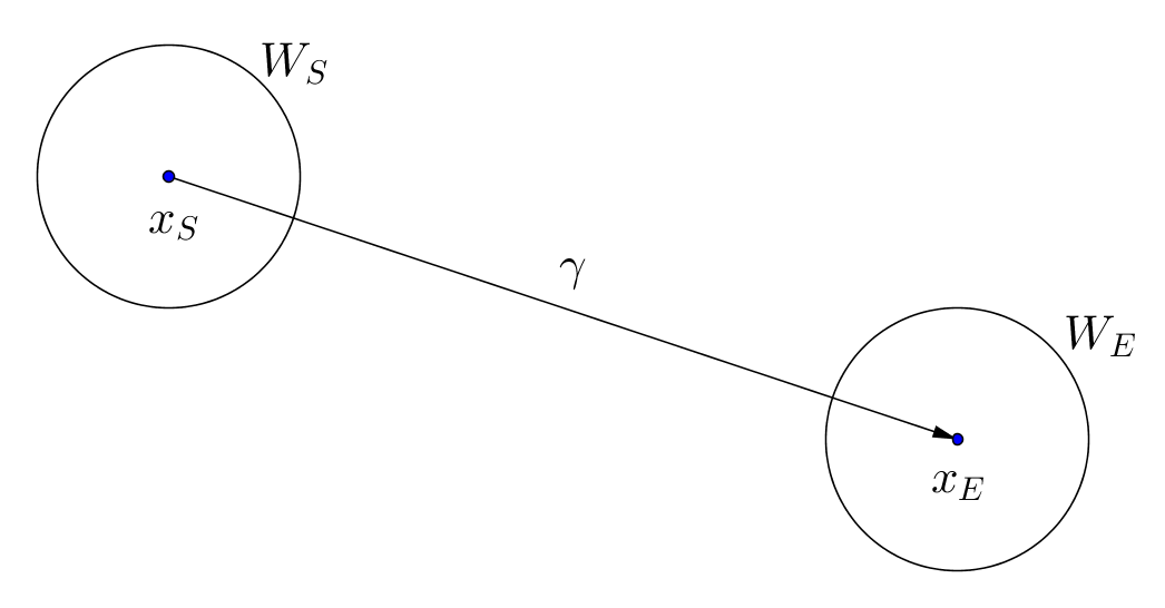
Figure 2. gradient flow line $\gamma$

We consider an input form $\zeta_{S}$ defined in a neighborhood $W_{S}$ of $x_{S}$. Suppose we are given a WKB approximation of $\zeta_{S}$ in $W_{S}$, which is an approximation of $\zeta_{S}$ according to order of $\lambda$ of the form

(3.2) $$\zeta_{S}\sim e^{-\lambda g_{\scalebox{0.7}{$\scriptscriptstyle S$}}}(\omega_{S,0}+\omega_{S,1}\lambda^{-1/2}+\omega_{S,2}\lambda^{-1}+\dots)$$

which means we have $\lambda_{j,0}>0$ such that when $\lambda>\lambda_{j,N,0}$ we have

$$\|e^{\lambda g_{\scalebox{0.7}{$\scriptscriptstyle S$}}}\nabla^{j}(\zeta_{S}-e^{-\lambda g_{\scalebox{0.7}{$\scriptscriptstyle S$}}}(\sum_{i=0}^{N}\omega_{S,i}\lambda^{-i/2}))\|^{2}_{L^{\infty}(W_{S})}\leq C_{j,N}\lambda^{-N-1+2j},$$

for any $j,N\in\mathbb{Z}_{+}$. We further assume that $g_{S}$ is a nonnegative Bott-Morse function in $W_{S}$ with zero set $V_{S}$ such that $\gamma$ is not tangent to $V_{S}$ at $x_{S}$. We consider the equation

(3.3) $$\Delta_{ij}\zeta_{E}=(I-P_{ij})d_{ij}^{*}(\chi_{S}\zeta_{S}),$$

where $\chi_{S}$ is a cutoff function compactly supported in $W_{S}$, $P_{ij}:\Omega^{*}(M)\rightarrow\Omega_{ij,<1}^{*}$ is the projection. We want to have a WKB approximation of $\zeta_{E}=H_{ij}(\chi_{S}\zeta_{S})$

Lemma 3.11.

For $\operatorname{supp}(\chi_{S})$ small enough (the size only depends on $g_{S}$ and $f_{ij}$), there is a WKB approximation of $\zeta_{E}$ in a small enough neighborhood $W_{E}$ of $x_{E}$, of the form $\zeta_{E}\sim e^{-\lambda g_{\scalebox{0.7}{$\scriptscriptstyle E$}}}\lambda^{-1/2}(\omega_{E,0}+\omega_{E,1}\lambda^{-1/2}+\dots)$ in the sense that we have $\lambda_{j,0}>0$ such that when $\lambda>\lambda_{j,N,0}$ we have

$$\|e^{\lambda g_{\scalebox{0.7}{$\scriptscriptstyle E$}}}\nabla^{j}\{\zeta_{E}-e^{-\lambda g_{\scalebox{0.7}{$\scriptscriptstyle E$}}}(\sum_{i=0}^{N}\omega_{E,i}\lambda^{-(i+1)/2})\}\|^{2}_{L^{\infty}(W_{E})}\leq C_{j,N}\lambda^{-N+2j}.$$

Furthermore, the function $g_{E}$ (only depending on $g_{S}$ and $f_{ij}$) is a nonnegative function which is Bott-Morse in $W_{E}$ with zero set $V_{E}=(\bigcup_{-\infty<t<+\infty}\varsigma_{t}(V_{S}))\cap W_{E}$ which is a closed submanifold in $W_{E}$, where $\varsigma_{t}$ is the $t$-time $\nabla f_{ij}/|\nabla f_{ij}|^{2}$.

Finally, we have the following Lemma 3.12 from [3] relating the integrals of $\omega_{S,0}$ and $\omega_{E,0}$.

Lemma 3.12.

Using same notations in lemma 3.11 and suppose $\chi_{S}$ and $\chi_{E}$ are cutoff functions supported in $W_{S}$ and $W_{E}$ respectively, then we have

(3.4) $$\lambda^{-\frac{1}{2}}\int_{N_{x_{E}}}e^{-\lambda g_{\scalebox{0.7}{$\scriptscriptstyle E$}}}\chi_{E}\omega_{E,0}=(\int_{N_{x_{S}}}e^{-\lambda g_{\scalebox{0.7}{$\scriptscriptstyle S$}}}\chi_{S}\omega_{S,0})(1+\mathcal{O}(\lambda^{-1})).$$

Furthermore, suppose $\omega_{S,0}(x_{S})\in\bigwedge^{top}N(V_{S})^{*}_{x_{S}}$, we have $\omega_{E,0}(x_{E})\in\bigwedge^{top}N(V_{E})^{*}_{x_{E}}$. Here $\bigwedge^{top}E$ refers to $\bigwedge^{r}E$ for a rank $r$ vector bundle $E$. Here $N_{v_{S}}$ and $N_{v_{E}}$ are any closed submanifold of $W_{S}$ and $W_{E}$ intersecting $V_{S}$ and $V_{E}$ transversally at $x_{S}$ and $x_{E}$ respectively.

3.2. Apriori Estimate

Notations 3.13.

From now on, we will consider a fixed generic sequence $\vec{f}=(f_{0},\dots,f_{k})$ with corresponding sequence of critical points $\vec{q}=(q_{(k-1)k},\dots,q_{01},q_{0k})$ and a fixed labeled ribbon $k$-tree $T$ such that $\dim(\mathcal{M}_{T}(\vec{f},\vec{q}))=0$ (the dimension is given by formula (2.2)). We use $q_{ij}$ to denote a fixed critical point of $f_{ij}$. $\phi(q_{ij})$ associated to $q_{ij}$ is abbreviated by $\phi_{ij}$.

Notations 3.14.

For $T\in\mathbb{T}_{k}$ or $\mathbb{L}\mathbb{T}_{k}$ with $\vec{q}$, we let $\blacktriangle_{T}:=\prod_{v\in LT^{[0]}}\blacktriangle_{\nu(v)}$ of dimension $\nu(T):=\sum_{v\in LT^{[0]}}\nu(v)$, and we also let $\deg(T):=\sum_{i=0}^{k-1}\deg(q_{i(i+1)})-|T^{[1]}|-\nu(T)$. We inductively define a volume form $\nu_{T}$ on $\blacktriangle_{T}$ for labeled ribbon tree $T\in\mathbb{L}\mathbb{T}_{k}$ by: letting $\nu_{l}=dt_{l}\wedge\cdots\wedge dt_{1}$ on the $\blacktriangle_{l}$; and for $v_{r}$ labeled with $1$ we split $T$ at $v_{r}$ into $T_{2}$ and $T_{1}$ such that $T_{2},T_{1},e_{o}$ is clockwisely oriented, then we take $\nu_{T}=\nu_{T_{2}}\wedge\nu_{T_{1}}$; and for $v_{r}$ labeled with $u$ we split $T$ at $v_{r}$ into $T_{l},\dots,T_{1}$ clockwisely, and we take $\nu_{T}=\nu_{T_{l}}\wedge\cdots\wedge\nu_{T_{1}}\wedge\nu_{l}$. We should also write $\nu_{T}^{\vee}$ to be the polyvector field dual to $\nu_{T}$.

Definition 3.15.

Given a labeled ribbon $k$-tree $T$ with $\vec{f}$ and $\vec{q}$ as above, we associate to it a length function $\hat{\rho}_{T}$ on $\mathfrak{M}(T):=\blacktriangle_{T}\times M^{|T^{[0]}_{ni}|}\rightarrow{}_{+}$ with coordinates $(\vec{\mathbf{t}}_{T},\hat{x}_{T})$ (where $\vec{\mathbf{t}}_{T}=(\mathbf{t}_{v})_{v\in LT^{[0]}}$ and $\hat{x}_{T}=(x_{v})_{v\in T^{[0]}_{ni}}$) inductively along the tree by the rules:

1. for the unique tree with one edge $e$ numbered by $ij$, we take $\hat{\rho}_{T}(x_{v_{o}}):=\rho_{ij}(q_{ij},x_{v_{o}})$;

2. when $v_{r}$ is labeled with $1$, we split $T$ at the root vertex $v_{r}$ into $T_{2},T_{1}$. We notice that $\mathfrak{M}(T)=\mathfrak{M}(T_{2})\times_{M}\mathfrak{M}(T_{1})\times M_{v_{o}}$ (with coordinates $\vec{\mathbf{t}}_{T}=(\vec{\mathbf{t}}_{T_{2}},\vec{\mathbf{t}}_{T_{1}})$, and $\hat{x}_{T}=(\hat{x}_{T_{2}},\hat{x}_{T_{1}},x_{v_{o}})$ such that $x_{T_{2},v_{r}}=x_{T_{1},v_{r}}=x_{v_{r}}$ in $M$) and we let

   $$\hat{\rho}_{T}(\vec{\mathbf{t}}_{T},\hat{x}_{\digamma(T)})=\hat{\rho}_{ij}(x_{v_{r}},x_{v_{o}})+\sum_{j=1}^{2}\hat{\rho}_{T_{j}}(\vec{\mathbf{t}}_{T_{j}},\hat{x}_{T_{j}})$$

   if the numbering on $e_{o}$ is $ij$;

3. when $v_{r}$ is labeled with $u$, we split $T$ at $v_{r}$ into $T_{l},\dots,T_{1}$ and we can write $\mathfrak{M}(T)=\mathfrak{M}_{T_{l}}\times_{M}\cdots\times_{M}\mathfrak{M}(T_{1})\times_{M}(\blacktriangle_{l}\times M_{v_{r}})\times M_{v_{o}}$ where $l=\nu(v_{r})$. By writing coordinates $(\vec{\mathbf{t}}_{T_{j}},\hat{x}_{T_{j}})$ for $\mathfrak{M}(T_{j})$, $\mathbf{t}_{v_{r}}=(t_{v_{r},l},\dots,t_{v_{r},1})$ for $\blacktriangle_{l}$, $x_{v_{r}}$ for $M_{v_{r}}$ and $x_{v_{o}}$ for $M_{v_{o}}$ satisfying $x_{T_{l},v_{r}}=\sigma_{t_{v_{r},l}}(x_{v_{r}}),\cdots,x_{T_{1},v_{r}}=\sigma_{t_{v_{r},1}}(x_{v_{r}})$, we let

   $$\hat{\rho}_{T}(\vec{\mathbf{t}}_{T},\hat{x}_{T}):=\hat{\rho}_{ij}(x_{v_{r}},x_{v_{o}})+\sum_{j=1}^{l}\hat{\rho}_{T_{j}}\big{(}\vec{\mathbf{t}}_{T_{j}},\hat{x}_{T_{j}}\big{)}$$

   if the numbering on $e_{o}$ is $ij$.

Fixing the outgoing point $x_{v_{o}}=q_{0k}$ giving coordinates $\vec{x}_{T}=(x_{v})_{v\in T^{[0]}}$ for $M^{|T^{[0]}|}$, we let $\rho_{T}(\vec{\mathbf{t}}_{T},\vec{x}_{T}):=\hat{\rho}_{T}(\vec{\mathbf{t}}_{T},\vec{x}_{T},q_{0k})$.

Example 3.16.

Suppose that $T$ is the labeled ribbon $2$-tree with two incoming vertices $v_{2}$ and $v_{1}$ joining to $v$ labeled with $u$ by $e_{12}$ and $e_{01}$, and $v$ is joining to the root vertex $v_{r}$ labeled with $u$ via $e$. Then we have $\blacktriangle_{T}\times M^{|T^{[0]}_{ni}|}=\blacktriangle_{2}\times\mathbb{S}^{1}\times M^{3}$ and $\hat{\rho}_{T}(t_{v,2},t_{v,1},t_{v_{r}},x_{v},x_{v_{r}},x_{v_{o}})=\rho_{02}(x_{v_{r}},x_{v_{o}})+\rho_{02}(x_{v},\sigma_{t_{v_{r}}}(x_{v_{r}}))+\rho_{12}(q_{12},\sigma_{t_{v,2}}(x_{v}))+\rho_{01}(q_{01},\sigma_{t_{v,1}}(x_{v}))$. The following Figure 3 shows the tree $T$ and its associated $\hat{\rho}_{T}$.

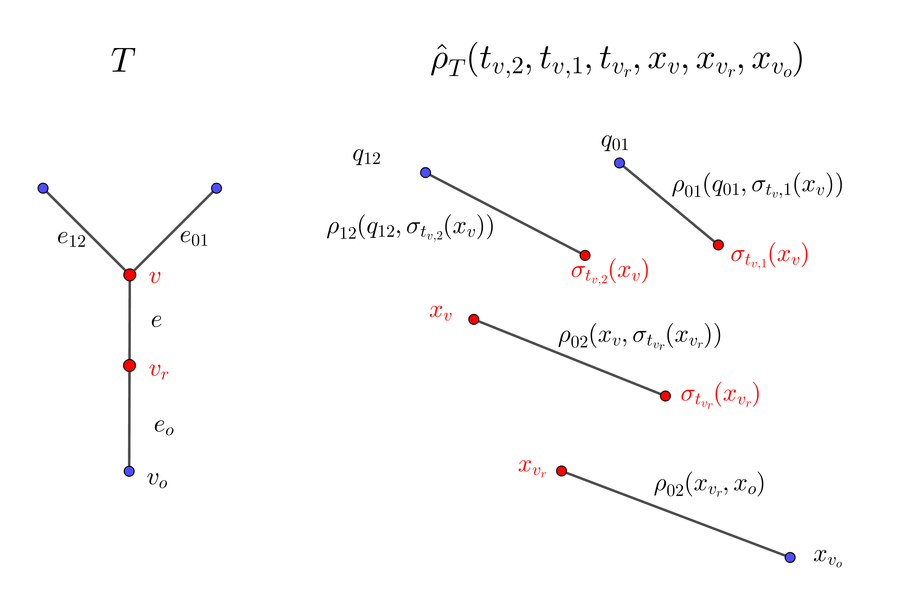
Figure 3. Distance function associated to $T$

From its construction and Lemma 3.3, we notice that $\rho_{T}(\vec{\mathbf{t}}_{T},\vec{x}_{T})\geq 0$ and equality holds if and only if for each edge $e$ numbered by $ij$ with $\partial_{in}(e)=v_{1}$ and $\partial_{o}(e)=v_{2}$, there is a generalized flow line of $\nabla f_{ij}$ joining $x_{v_{1}}$ to $\tilde{x}_{v_{2}}$, where $\tilde{x}_{v_{2}}=x_{v_{2}}$ when $v_{2}$ is labeled by $1$; and $\tilde{x}_{v_{2}}=\sigma_{t_{v_{2},j}}(x_{v_{2}})$ if $v_{2}$ is labeled by $u$ with and $e$ is the $j^{\text{th}}$ incoming edges of $v_{2}$ in the anti-clockwise orientation. Therefore, we have a generalized flow tree (with jumping) of type $(T,\vec{f},\vec{q})$ (which is a generalization of flow tree in Definition 2.7 by allow broken flow lines as in Definition 3.3). With the condition that $\dim(\mathcal{M}(\vec{f},\vec{q}))=0$ as mentioned in Notation 3.13, we notice that every such generalized flow line is an actual flow line from the generic assumption 2.8 for $\vec{f}$, because the expected dimension for flow tree with broken flow line is negative.

Notations 3.17.

We let $\Gamma_{1},\dots,\Gamma_{d}$ be the gradient flow tree of type $(T,\vec{f},\vec{q})$, such that each $\Gamma_{i}$ is associated with a point $\mathbf{t}_{\Gamma_{i},v}\in\blacktriangle_{\nu(v)}$ (for $v\in LT^{[0]}$) and $x_{\Gamma_{i},v}\in M$ (for $v\in T^{[0]}$) such that

1. $x_{\Gamma_{i},v}$ is the starting point of a gradient flow line $\gamma_{e}$ associated to edge $e$ if $\partial_{in}(e)=v$, and we write $x_{\Gamma_{i},e,v}=x_{\Gamma_{i},v}$ in this case;

2. $x_{\Gamma_{i},v}$ is the end point of the gradient flow line $\gamma_{e}$ if $v$ is labeled by $1$ if $\partial_{o}(e)=v$, and we write $x_{\Gamma_{i},e,v}=x_{\Gamma_{i},v}$ in this case;

3. and $\sigma_{t_{\Gamma_{i},v,j}}(x_{\Gamma_{i},v})$ is the end point of a gradient flow line $\gamma_{e}$ associated to $j^{th}$-edge $e$ clockwisely if $v$ is labeled by $u$ and $\partial_{o}(e)=v$, and we write $x_{\Gamma_{i},e,v}=\sigma_{t_{\Gamma_{i},v,j}}(x_{\Gamma_{i},v})$ in this case.

We consider a sequence of cut off functions $\vec{\chi}:=(\chi_{v})_{v\in T^{[0]}}$ such that $\chi_{v}$ compactly supported in a ball $U_{v}:=B(x_{v},r/2)$ of radius $r$ centered at a fixed point $x_{v}\in M$, and $(\vec{\varkappa}_{v})_{v\in LT^{[0]}}$ with $\varkappa_{v}$ compactly support in a small neighborhood $\mathbf{C}_{v}$ containing a fixed $\mathbf{t}_{v}=(t_{v,\nu(v)},\dots,t_{v,1})\in\blacktriangle_{\nu(v)}$ such that the Riemannian distance between $\sigma_{t_{j}}(x)$ and $\sigma_{t^{\prime}_{j}}(x)$ is strictly less than $r/2$ for any $j$ and any $x\in M$ and any $\mathbf{t}$ and $\mathbf{t}^{\prime}$ in $\mathbf{C}_{v}$.

Definition 3.18.

With $\vec{\chi}$ and $\vec{\varkappa}$ as above, we define $\mathfrak{m}^{(e,v)}_{\vec{\chi},\vec{\varkappa}}\in\Omega^{*}(\blacktriangle_{T_{e,v}}\times M)$ for each flag $(e,v)\in\digamma(T)$ inductively along $T$ by letting:

1. for the incoming edge $e_{ij}$ with $\partial_{o}(e_{ij})=v$, we take $\mathfrak{m}^{(e_{ij},v)}_{\vec{\chi},\vec{\varkappa}}=\phi_{ij}$;

2. when we have $(e,v)$ with $\partial_{in}(e)=v$ with $v$ is labeled with $1$ with, we let $T_{2},T_{1}$ to be subtrees with outgoing edges $e_{2},e_{1}$ ending at $v$ such that $e_{2},e_{1},e$ clockwisely oriented. With coordinates $\vec{\mathbf{t}}_{T_{e,v}}=(\vec{\mathbf{t}}_{T_{2}},\vec{\mathbf{t}}_{T_{1}})$ for $\blacktriangle_{T}=\blacktriangle_{T_{2}}\times\blacktriangle_{T_{1}}$, we let

   $$\mathfrak{m}^{(e,v)}_{\vec{\chi},\vec{\varkappa}}(\vec{\mathbf{t}}_{T_{e,v}},x)=(-1)^{\varepsilon}\nu_{T_{e,v}}\chi_{v_{r}}(x)\big{(}\iota_{\nu_{T_{2}}^{\vee}}\mathfrak{m}^{(e_{2},v)}_{\vec{\chi},\vec{\varkappa}}(\vec{\mathbf{t}}_{T_{2}},x)\big{)}\wedge\big{(}\iota_{\nu_{T_{1}}^{\vee}}\mathfrak{m}^{(e_{1},v)}_{\vec{\chi},\vec{\varkappa}}(\vec{\mathbf{t}}_{T_{1}},x)\big{)},$$

   where $\varepsilon=\deg\big{(}\iota_{\nu_{T_{2}}^{\vee}}\mathfrak{m}^{(e_{2},v)}_{\vec{\chi},\vec{\varkappa}}(\vec{\mathbf{t}}_{T_{2}},x)\big{)}+1$;

3. when we have $v$ labeled with $u$, we let $T_{l},\dots,T_{1}$ be subtrees with outgoing edges $e_{l},\dots,e_{1}$ ending at $v$ with $e_{l},\dots,e_{1},e$ clockwisely oriented. We let

   $$\mathfrak{m}^{(e,v)}_{\vec{\chi},\vec{\varkappa}}(\vec{\mathbf{t}}_{T_{e,v}},x)=\nu_{T_{e,v}}\chi_{v}(x)\varkappa_{v}(\mathbf{t}_{v})\sigma_{t_{v,l}}^{*}\big{(}\iota_{w_{v,l}\wedge\nu_{T_{l}}^{\vee}}\mathfrak{m}^{(e_{l},v)}_{\vec{\chi},\vec{\varkappa}}(\vec{\mathbf{t}}_{T_{l}},x)\big{)}\wedge\cdots\wedge\sigma_{t_{v,1}}^{*}\big{(}\iota_{w_{v,1}\wedge\nu_{T_{1}}^{\vee}}\mathfrak{m}^{(e_{1},v)}_{\vec{\chi},\vec{\varkappa}}(\vec{\mathbf{t}}_{T_{1}},x)\big{)},$$

   where $t_{v,l},\dots,t_{v,1}$ is the coordinates for $\blacktriangle_{\nu(v)}$ and $\vec{\mathbf{t}}_{T_{e,v}}=(\vec{\mathbf{t}}_{T_{l}},\dots,\vec{\mathbf{t}}_{T_{1}},t_{v,l},\dots,t_{v,1})$, and $w_{v,j}=\sigma_{*}(\frac{\partial}{\partial t_{v,j}})$;

4. for an edge $e$ numbered by $ij$ with $\partial_{in}(e)=v_{0}$ and $\partial_{o}(e)=v_{1}$ with $v_{1}$ not being the outgoing vertex $v_{o}$, we let $\mathfrak{m}^{(e,v_{1})}_{\vec{\chi},\vec{\varkappa}}=d^{*}_{ij}G_{ij}(\mathfrak{m}^{(e,v_{0})}_{\vec{\chi},\vec{\varkappa}})$ where $G_{ij}$ is introduced in Definition 2.4;

5. for the outgoing edge $e_{o}$ with $\partial_{in}(e_{o})=v_{r}$ and $\partial_{o}(e_{o})=v_{o}$, we take $\mathfrak{m}^{T}_{\vec{\chi},\vec{\varkappa}}=\mathfrak{m}^{(e_{o},v_{o})}_{\vec{\chi},\vec{\varkappa}}=\mathfrak{m}^{(e_{o},v_{r})}_{\vec{\chi},\vec{\varkappa}}$.

Example 3.19.

We the tree $T$ described in the previous Example 3.16, we have $\mathfrak{m}^{(e,v)}_{\vec{\chi},\vec{\varkappa}}(t_{v,2},t_{v,1},x_{v})=\chi_{v}(x_{v})\varkappa_{v}(t_{v,2},t_{v,1})dt_{v,2}dt_{v,1}\sigma_{t_{v_{2}}}^{*}(\iota_{w_{v,2}}\phi_{02})(x_{v})\wedge\sigma_{t_{v_{1}}}^{*}(\iota_{w_{v,1}}\phi_{01})(x_{v})$, $\mathfrak{m}^{(e,v_{r})}_{\vec{\chi},\vec{\varkappa}}=d^{*}_{02}G_{02}(\mathfrak{m}^{(e,v)}_{\vec{\chi},\vec{\varkappa}})$ ($d^{*}_{02}G_{02}$ only acting on the component $M$) and

$$\mathfrak{m}^{(e_{o},v_{r})}_{\vec{\chi},\vec{\varkappa}}(t_{v,2},t_{v,1},t_{v_{r}},x_{v_{r}})=\chi_{v_{r}}(x_{v_{r}})\varkappa(t_{v_{r}})dt_{v,2}dt_{v,1}dt_{v_{r}}\sigma_{t_{v_{r}}}^{*}(\iota_{w_{v_{r}}\wedge\frac{\partial}{\partial t_{v,1}}\wedge\frac{\partial}{\partial t_{v,2}}}\mathfrak{m}^{(e,v_{r})}_{\vec{\chi},\vec{\varkappa}})(x_{v_{r}}),$$

and finally we have $\mathfrak{m}^{T}_{\vec{\chi},\vec{\varkappa}}=\mathfrak{m}^{(e_{o},v_{r})}_{\vec{\chi},\vec{\varkappa}}$.

We take a collection $\{\vec{\chi}_{\mathbf{i}}\}_{\mathbf{i}\in\mathscr{I}}$ and $\{\vec{\varkappa}_{\mathbf{j}}\}_{\mathbf{j}\in\mathscr{J}}$ such that $\vec{\chi}_{\mathbf{i}}=(\chi_{i,v})_{\begin{subarray}{c}i\in\mathscr{I}_{v}\\ v\in T^{[0]}\end{subarray}}$ and $\vec{\varkappa}_{\mathbf{j}}=(\varkappa_{j,v})_{\begin{subarray}{c}j\in\mathscr{J}_{v}\\ v\in LT^{[0]}\end{subarray}}$ and such that every collection $\{\chi_{i,v}\}_{i\in\mathscr{I}_{v}}$ and $\{\varkappa_{j,v}\}_{j\in\mathscr{J}_{v}}$ is a partition of unity for $M_{v}$ and $\blacktriangle_{\nu(v)}$ respectively (Here we use the notation $\mathscr{I}=\prod_{v\in T^{[0]}}\mathscr{I}_{v}$ and $\mathscr{J}=\prod_{v\in T^{[0]}}\mathscr{J}_{v}$). With the cut off construction in Definition 3.18 and the Definition 2.4, we have

(3.5) $$\int_{M}m_{k,T}(\lambda)(\phi_{(k-1)k},\dots,\phi_{01})\wedge\frac{\ast e^{-2\lambda f_{0k}}\phi_{0k}}{\|e^{-\lambda f_{0k}}\phi_{0k}\|^{2}}=\sum_{\mathbf{i}\in\mathscr{I}}\sum_{\mathbf{j}\in\mathscr{J}}\int_{\blacktriangle_{T}\times M}\mathfrak{m}^{T}_{\vec{\chi}_{\mathbf{i}},\vec{\varkappa}_{\mathbf{j}}}\wedge\frac{\ast e^{-2\lambda f_{0k}}\phi_{0k}}{\|e^{-\lambda f_{0k}}\phi_{0k}\|^{2}}.$$

Lemma 3.20.

We fix a point $(\vec{\mathbf{t}}_{T},\vec{x}_{T})$ in $\mathfrak{M}(T)$ with the cut off functions $\vec{\chi}$ and $\vec{\varkappa}$ and $\mathfrak{m}^{T}_{\vec{\chi},\vec{\varkappa}}$ as before Definition 3.18, for any $\epsilon>0$ we have $\lambda_{0}(\epsilon)$ and small enough radius $r=r(\epsilon)$ of cut off functions (which is described before Definition 3.18) such that when $\lambda>\lambda_{0}$ we have the norm estimate

$$\|\mathfrak{m}^{T}_{\vec{\chi},\vec{\varkappa}}\wedge\frac{\ast e^{-2\lambda f_{0k}}\phi_{0k}}{\|e^{-\lambda f_{0k}}\phi_{0k}\|^{2}}\|_{C^{j}(\blacktriangle_{T}\times M)}\leq C_{j,\epsilon}e^{-\lambda(\rho_{T}(\vec{\mathbf{t}}_{T},\vec{x}_{T})-b_{T}\epsilon)},$$

for any $j\in\mathbb{Z}_{+}$ (Here we fix an arbitrary metric on the simplices $\blacktriangle_{l}$’s), where $b_{T}$ is a constant depending the combinatorics of $T$.

Proof.

We prove by induction along the tree $T$ that for each flag $(e,v)$ with $\partial_{o}(e)=v\neq v_{o}$ we have

$$\|\mathfrak{m}^{(e,v)}_{\vec{\chi},\vec{\varkappa}}\|_{C^{j}(\blacktriangle_{T_{e,v}}\times U_{v})}\leq C_{j,\epsilon,\vec{\chi},\vec{\varkappa}}\exp\left(-\lambda(\hat{\rho}_{T_{e,v}}(\vec{\mathbf{t}}_{T_{e,v}},\hat{x}_{T_{e,v}})-b_{T_{e,v}}\epsilon)\right),$$

where $U_{v}=B(x_{v},r/2)$, for any points $\vec{\mathbf{t}}_{T}\in\blacktriangle_{T}$, $\hat{x}_{T}\in M^{|T^{[0]}_{ni}|}$ with the assoicated cut off functions $\vec{\varkappa}$ and $\vec{\chi}$ with small enough $r$. The initial case follows from the estimate in Lemma 3.6. For induction we consider an edge $e$ with $\partial_{in}(e)=v$ and $\partial_{o}(e)=\tilde{v}$. We take subtrees (of $T$) $T_{l},\dots,T_{1}$ with edges $e_{l},\dots,e_{1}$ attached to $v$ such that $e_{l},\dots,e_{1},e$ is clockwisely oriented. There are two cases.

The first case is when $v$ is labeled with $1$ and we have $l=2$. In this case we have the estimate

$$\|\mathfrak{m}^{(e_{2},v)}_{\vec{\chi},\vec{\varkappa}}\wedge\mathfrak{m}^{(e_{1},v)}_{\vec{\chi},\vec{\varkappa}}\|_{C^{j}(\blacktriangle_{T_{e_{2},v}}\times\blacktriangle_{T_{e_{1},v}}\times U_{v})}\leq C_{j,\epsilon,\vec{\chi},\vec{\varkappa}}\exp\left(-\lambda\big{(}\hat{\rho}_{T_{2}}(\vec{\mathbf{t}}_{T_{2}},\hat{x}_{T_{2}})+\hat{\rho}_{T_{1}}(\vec{\mathbf{t}}_{T_{1}},\hat{x}_{T_{1}})-b_{T_{e,v}}\epsilon\big{)}\right)$$

by choosing $b_{T_{e,v}}\geq b_{T_{1}}+b_{T_{2}}$, where we require $x_{T_{1},v}=x_{T_{2},v}=x_{v}$ in the R.H.S. of the above equation. Assuming that $e$ is numbered by $ij$, and we apply the Lemma 3.5 to the term $\mathfrak{m}^{(e,\tilde{v})}_{\vec{\chi},\vec{\varkappa}}=d^{*}_{ij}G_{ij}\big{(}\chi_{v}\mathfrak{m}^{(e_{2},v)}_{\vec{\chi},\vec{\varkappa}}\wedge\mathfrak{m}^{(e_{1},v)}_{\vec{\chi},\vec{\varkappa}}\big{)}$ (we choose smaller $r$ if necessary) we obtain the estimate

$$\|d^{*}_{ij}G_{ij}\big{(}\chi_{v}\mathfrak{m}^{(e_{2},v)}_{\vec{\chi},\vec{\varkappa}}\wedge\mathfrak{m}^{(e_{1},v)}_{\vec{\chi},\vec{\varkappa}}\big{)}\|_{C^{j}(\blacktriangle_{T_{e,\tilde{v}}}\times U_{\tilde{v}})}\leq C_{j,\epsilon,\vec{\chi},\vec{\varkappa}}\exp\left(-\lambda\big{(}\hat{\rho}_{T_{e,\tilde{v}}}(\vec{\mathbf{t}}_{T_{e,\tilde{v}}},\hat{x}_{T_{e,\tilde{v}}})-b_{T_{e,\tilde{v}}}\epsilon\big{)}\right),$$

by taking $b_{T_{e,\tilde{v}}}\geq b_{T_{e,v}}+1$ which is the desired estimate.

The second case is when $v$ is labeled with $u$, and we have the estimate

$$\|\sigma^{*}_{t_{l}}\big{(}\iota_{w_{v,l}\wedge\nu_{T_{l}}^{\vee}}\mathfrak{m}^{(e_{l},v)}_{\vec{\chi},\vec{\varkappa}}\big{)}\wedge\cdots\wedge\sigma^{*}_{t_{1}}\big{(}\iota_{w_{v,1}\wedge\nu_{T_{1}}^{\vee}}\mathfrak{m}^{(e_{1},v)}_{\vec{\chi},\vec{\varkappa}}\big{)}\|_{C^{j}(\prod_{j=1}^{l}\blacktriangle_{T_{j}}\times\mathbf{C}_{v}\times U_{v})}\\ \leq C_{j,\epsilon,\vec{\chi},\vec{\varkappa}}\exp\left(-\lambda\big{(}\sum_{j=1}^{l}\hat{\rho}_{T_{j}}(\vec{\mathbf{t}}_{T_{j}},\hat{x}_{T_{j}})-b_{T_{e,v}}\epsilon\big{)}\right),$$

using the induction hypothesis and by taking $b_{T_{e,v}}\geq l+\sum_{j=1}^{l}b_{T_{j}}$, for $(t_{l},\dots,t_{1})$ varying in small enough neighborhood $\mathbf{C}_{v}$ of $(t_{v,l},\dots,t_{v,1})$ ($\mathbf{C}_{v}$ introduced in the paragraph before Definition 3.18), where we require that the identity $x_{T_{j},v}=\sigma_{t_{v,j}}(x_{v})$ on the R.H.S. as in the Definition 3.15. By applying $d^{*}_{ij}G_{ij}$ (if $e$ is numbered by $ij$) to the term $\mathfrak{m}^{(e,v)}_{\vec{\chi},\vec{\varkappa}}=\nu_{T_{e,v}}\chi_{v}\varkappa_{v}\sigma^{*}_{t_{l}}\big{(}\iota_{w_{v,l}\wedge\nu_{T_{l}}^{\vee}}\mathfrak{m}^{(e_{l},v)}_{\vec{\chi},\vec{\varkappa}}\big{)}\wedge\cdots\wedge\sigma^{*}_{t_{1}}\big{(}\iota_{w_{v,1}\wedge\nu_{T_{1}}^{\vee}}\mathfrak{m}^{(e_{1},v)}_{\vec{\chi},\vec{\varkappa}}\big{)}$ as in Definition 3.18, and using Lemma 3.5 again we have the desired estimate

$$\|\mathfrak{m}^{(e,\tilde{v})}_{\vec{\chi},\vec{\varkappa}}\|_{C^{j}(\blacktriangle_{T_{e,\tilde{v}}}\times U_{\tilde{v}})}\leq C_{j,\epsilon,\vec{\chi},\vec{\varkappa}}\exp\left(-\lambda\big{(}\hat{\rho}_{T_{e,\tilde{v}}}(\vec{\mathbf{t}}_{T_{e,\tilde{v}}},\hat{x}_{T_{e,\tilde{v}}})-b_{T_{e,\tilde{v}}}\epsilon\big{)}\right),$$

where we take $b_{T_{e,\tilde{v}}}\geq b_{T_{e,v}}+1$.

To obtain the statement of the Lemma, we observe that if $T_{l},\cdots,T_{1}$ are the incoming trees joining to the root vertex we have

$$\|\mathfrak{m}^{(e_{o},v_{o})}_{\vec{\chi},\vec{\varkappa}}\|_{C^{j}(\blacktriangle_{T}\times U_{v_{r}})}\leq C_{j,\epsilon,\vec{\chi},\vec{\varkappa}}\exp\left(-\lambda\big{(}\sum_{j=1}^{l}\hat{\rho}_{T_{j}}(\vec{\mathbf{t}}_{T_{j}},\hat{x}_{T_{j}})-b_{T_{e_{o},v_{o}}}\epsilon\big{)}\right)$$

in a small enough neighborhood $U_{v_{r}}$ of $x_{v_{r}}$, where we have $l=2$ and $x_{T_{2},v_{r}}=x_{T_{1},v_{r}}=x_{v_{r}}$ in R.H.S. as in the first case with $v_{r}$ labeled with $1$, and $x_{T_{j},v_{r}}=\sigma_{t_{v_{r},j}}(x_{v_{r}})$ in R.H.S. as in the second case that $v_{r}$ is labeled with $u$. The Lemma follows from the estimate for $\mathfrak{m}^{(e_{o},v_{o})}_{\vec{\chi},\vec{\varkappa}}$ and that for $\frac{\ast e^{-2\lambda f_{0k}}\phi_{0k}}{\|e^{-\lambda f_{0k}}\phi_{0k}\|^{2}}$ in Remark 3.7. ∎

The above Lemma allows us to estimate the terms $\mathfrak{m}^{T}_{\vec{\chi},\vec{\varkappa}}$ appearing in the R.H.S., and from the discussion after Example 3.16 we notice that it is closely related to gradient flow tree of type $T$. With the gradient flow trees $\Gamma_{i}$’s as in Notation 3.17, we assume there are open neighborhoods $D_{\Gamma_{i},v}$ and $W_{\Gamma_{i},v}$ of $x_{\Gamma_{i},v}$ for $v\in T^{[0]}$ such that $\overline{D_{\Gamma_{i},v}}\subset W_{\Gamma_{i},v}$ together with $\chi_{\Gamma_{i},v}\equiv 1$ on $\overline{D_{\Gamma_{i},v}}$ which is compactly supported in $W_{\Gamma_{i},v}$ giving $\vec{\chi}_{\Gamma_{i}}=(\chi_{\Gamma_{i},v})_{v\in T^{[0]}}$. Similarly, we also assume there are open neighborhoods $\mathbf{C}_{\Gamma_{i},v}$ and $\mathbf{E}_{\Gamma_{i},v}$ of $\mathbf{t}_{\Gamma_{i},v}$ in $\blacktriangle_{\nu(v)}$ satisfying $\overline{\mathbf{C}_{\Gamma_{i},v}}\subset\mathbf{E}_{\Gamma_{i},v}$ together with $\varkappa_{\Gamma_{i},v}\equiv 1$ on $\overline{\mathbf{C}_{\Gamma_{i},v}}$ which is compactly supported in $\mathbf{E}_{\Gamma_{i},v}$ giving $\vec{\varkappa}_{\Gamma_{i}}=(\varkappa_{\Gamma_{i},v})_{v\in LT^{[0]}}$. We should further prescribe the size of these neighborhood $W_{\Gamma_{i},v}$’s and $\mathbf{E}_{\Gamma_{i},v}$ in the upcoming Section 3.3 which is defined along the gradient tree $\Gamma_{i}$’s together with the WKB approximation . By writing $\overline{\vec{D}_{\Gamma_{i}}}=\prod_{v\in T^{[0]}}\overline{D_{\Gamma_{i},v}}$ and $\overline{\vec{\mathbf{C}}_{\Gamma_{i}}}=\prod_{v\in LT^{[0]}}\overline{\mathbf{C}_{\Gamma_{i},v}}$, we have $\rho_{T}\geq c>0$ for some constant $c$ outside $\bigcup_{i=1}^{d}\overline{\vec{\mathbf{C}}_{\Gamma_{i}}}\times\overline{\vec{D}_{\Gamma_{i}}}$ by continuity of $\rho_{T}$ and the discussion after Example 3.16. As a result, we can fix a small enough $\epsilon$ (and the associated $r(\epsilon)$) such that $b_{T}\epsilon<c/2$. The following Figure 4 show the situation for these open subsets $W_{\Gamma_{i},v}$’s and $\mathbf{E}_{\Gamma_{i},v}$’s for the tree in Example 3.16.

Figure 4. Open subsets near gradient tree $\Gamma_{i}$

We can take a finite collection $\{\vec{\chi}_{\mathbf{i}}\}_{\mathbf{i}\in\mathscr{I}}$ and $\{\vec{\varkappa}_{\mathbf{j}}\}_{\mathbf{j}\in\mathscr{J}}$ in the paragraph before Lemma 3.20 such that $\{\vec{\chi}_{\mathbf{i}}\}_{\mathbf{i}\in\mathscr{I}}\cup\{\vec{\chi}_{\Gamma_{1}},\dots,\vec{\chi}_{\Gamma_{d}}\}$ forms a partition of unity of $M^{|T^{[0]}|}$ and finite collection $\{\vec{\varkappa}_{\mathbf{j}}\}_{\mathbf{j}\in\mathscr{J}}\cup\{\vec{\varkappa}_{\Gamma_{1}},\dots,\vec{\varkappa}_{\Gamma_{d}}\}$ forms a partition of unity of $\blacktriangle_{T}$ respectively, further satisfying $\big{(}\text{Supp}(\vec{\chi}_{\mathbf{i}})\times\text{Supp}(\vec{\varkappa}_{\mathbf{j}})\big{)}\cap\overline{\vec{\mathbf{C}}_{\Gamma_{i}}}\times\overline{\vec{D}_{\Gamma_{i}}}=\emptyset$ for each flow tree $\Gamma_{i}$ and any $\mathbf{i},\mathbf{j}$. Therefore we have the estimate $\|\mathfrak{m}^{T}_{\vec{\chi}_{\mathbf{i}},\vec{\varkappa}_{\mathbf{j}}}\wedge\frac{\ast e^{-2\lambda f_{0k}}\phi_{0k}}{\|e^{-\lambda f_{0k}}\phi_{0k}\|^{2}}\|_{C^{0}(\blacktriangle_{T}\times M)}\leq C_{\epsilon,\vec{\chi}_{\mathbf{i}},\vec{\varkappa}_{\mathbf{j}}}e^{-\lambda c/2}$. As a conclusion of this Section 3.2, we have

(3.6) $$\int_{M}m_{k,T}(\lambda)(\phi_{(k-1)k},\dots,\phi_{01})\wedge\frac{\ast e^{-2\lambda f_{0k}}\phi_{0k}}{\|e^{-\lambda f_{0k}}\phi_{0k}\|^{2}}=\sum_{i=1}^{d}\int_{\blacktriangle_{T}\times M}\mathfrak{m}^{T}_{\vec{\chi}_{\Gamma_{i}},\vec{\varkappa}_{\Gamma_{i}}}\wedge\frac{\ast e^{-2\lambda f_{0k}}\phi_{0k}}{\|e^{-\lambda f_{0k}}\phi_{0k}\|^{2}}+\mathcal{O}(e^{-\lambda c/2}),$$

where $\mathcal{O}(e^{-\lambda c/2})$ refers to function in $\lambda$ bounded by $Ce^{-\lambda c/2}$ for some $C$. This cut off the contribution to integral near the gradient flow trees $\Gamma_{i}$’s.

3.3. WKB approximation method

3.3.1. WKB expansion for $\mathfrak{m}^{(e,v)}_{\vec{\chi},\vec{\varkappa}}$

We fix a particular gradient flow tree $\Gamma=\Gamma_{i}$ (we omit $i$ in our notations for the rest of this paper) and compute the contribution from the integral $\int_{\blacktriangle_{T}\times M}\mathfrak{m}^{T}_{\vec{\chi}_{\Gamma},\vec{\varkappa}_{\Gamma}}\wedge\frac{e^{-2\lambda f_{ij}}\ast\phi_{0k}}{\|e^{-\lambda f_{0k}}\phi_{0k}\|^{2}}$ in the above equation 3.6 using techniques from [3, Section 3].

We inductively define the open subset $W_{e,v}\subset M$ and $\mathbf{E}_{v}$ of $\mathbf{t}_{v}$ along the tree $\Gamma$, together with a WKB expansion of $\mathfrak{m}^{(e,v)}_{\vec{\chi},\vec{\varkappa}}$ in $\vec{\mathbf{E}}_{T_{e,v}}\times W_{e,v}=\prod_{v\in LT^{[0]}_{e,v}}\mathbf{E}_{v}\times W_{e,v}$ for each flag $(e,v)$ of $T$

(3.7) $$\mathfrak{m}^{(e,v)}_{\vec{\chi},\vec{\varkappa}}\sim\lambda^{r_{e,v}}e^{-\lambda g_{e,v}}\big{(}\omega_{(e,v),0}+\omega_{(e,v),1}\lambda^{-\frac{1}{2}}+\cdots\big{)},$$

which is a norm estimate (here we fix arbitrary metric on $\blacktriangle_{l}$ as before) in the sense of Lemma 3.11, where $g_{e,v}\in\mathcal{C}^{\infty}(\vec{\mathbf{E}}_{T_{e,v}}\times W_{e,v})$ is non-negative Bott-Morse function with zero set $V_{e,v}\subset\vec{\mathbf{E}}_{T_{e,v}}\times W_{e,v}$ and $\omega_{(e,v),i}\in\Omega^{*}(\vec{\mathbf{E}}_{T_{e,v}}\times W_{e,v})$ as follows:

1. for the incoming edges $e_{ij}$ with $\partial_{o}(e_{ij})=v$, we define $W_{e_{ij},v}$ to be a open subset of $x_{\Gamma,e_{ij},v}$ (We use the notation as in Notation 3.17) together with the WKB expansion for $\phi_{ij}$ in $W_{e_{ij},v}$ from Lemma 3.9, with $r_{e_{ij},v}=\frac{\deg(q_{ij})}{2}$ and $g_{e_{ij},v}=g^{+}_{q_{ij}}$. In this case we have $V_{e_{ij},v}=V_{q_{ij}}^{+}\cap W_{e_{ij},v}$ being the stable submanifold;

2. for $(e,v)$ with $\partial_{in}(e)=v$ with $v$ is labeled with $1$, we let $T_{2},T_{1}$ to be subtrees with outgoing edges $e_{2},e_{1}$ ending at $v$ such that $e_{2},e_{1},e$ clockwisely oriented, we let $\vec{\mathbf{E}}_{T_{e,v}}=\vec{\mathbf{E}}_{T_{2}}\times\vec{\mathbf{E}}_{T_{1}}$ and $W_{e,v}=W_{e_{2},v}\cap W_{e_{1},v}$, with the product WKB expansion as

   $$(-1)^{\varepsilon}\chi_{v}\mathfrak{m}^{(e_{2},v)}_{\vec{\chi},\vec{\varkappa}}\wedge\mathfrak{m}^{(e_{1},v)}_{\vec{\chi},\vec{\varkappa}}\sim\lambda^{r_{e,v}}e^{-\lambda g_{e,v}}\big{(}\omega_{(e,v),0}+\omega_{(e,v),1}\lambda^{-\frac{1}{2}}+\cdots\big{)}$$

   by taking $\lambda^{r_{e,v}}=\lambda^{r_{e_{2},v}+r_{e_{1},v}}$, $g_{e,v}=g_{e_{2},v}+g_{e_{1},v}$ and $\omega_{(e,v),l}=\sum_{i+j=l}\chi_{v}\omega_{(e_{2},v),i}\wedge\omega_{(e_{1},v),j}$ (Here $\varepsilon$ is given (2) in Definition 3.18). In this case we have $g_{e,v}$ being a non-negative Bott-Morse function in $\vec{\mathbf{E}}_{T_{e,v}}\times W_{e,v}$ with zero set $V_{e,v}=(V_{e_{2},v}\times\vec{\mathbf{E}}_{T_{1}})\cap(V_{e_{1},v}\times\vec{\mathbf{E}}_{T_{1}})$;

3. when we have $v$ labeled with $u$, we let $T_{l},\dots,T_{1}$ be subtrees with outgoing edges $e_{l},\dots,e_{1}$ ending at $v$ with $e_{l},\dots,e_{1},e$ clockwisely oriented, we let $\vec{\mathbf{E}}_{T_{e,v}}=\prod_{j=1}^{l}\vec{\mathbf{E}}_{T_{j}}\times\mathbf{C}_{v}$ and take $W_{e,v}$ (Here $\mathbf{C}_{v}$ is neighborhood of $\mathbf{t}_{\Gamma,v}$, and $W_{e,v}$ is a neighborhood of $x_{\Gamma,v}=x_{\Gamma,e,v}$) such that $\sigma_{t_{j}}(W_{e,v})\subset W_{e_{j},v}$ for each $j=1,\dots,l$ for $(t_{l},\dots,t_{1})\in\mathbf{C}_{v}$. Therefore we have the WKB expansion $\mathfrak{m}^{(e,v)}_{\vec{\chi},\vec{\varkappa}}\sim\lambda^{r_{e,v}}e^{-\lambda g_{e,v}}\big{(}\omega_{(e,v),0}+\omega_{(e,v),1}\lambda^{-\frac{1}{2}}+\cdots\big{)}$ by taking $r_{e,v}=\sum_{j=1}^{l}r_{e_{j},v}$, $g_{e,v}=\sum_{j=1}^{l}\tau_{j}^{*}(g_{e_{j},v})$ and

   $$\omega_{(e,v),m}=\sum_{i_{l}+\cdots+i_{1}=m}\nu_{T_{e,v}}\chi_{v}\varkappa_{v}\big{(}\iota_{\frac{\partial}{\partial t_{v,l}}\wedge\nu_{T_{l}}^{\vee}}\tau_{l}^{*}(\omega_{(e_{l},v),i_{l}})\big{)}\wedge\cdots\wedge\big{(}\iota_{\frac{\partial}{\partial t_{v,1}}\wedge\nu_{T_{1}}^{\vee}}\tau_{1}^{*}(\omega_{(e_{1},v),i_{1}})\big{)},$$

   where $\tau_{j}:\prod_{j=1}^{l}\vec{\mathbf{E}}_{T_{j}}\times\blacktriangle_{\nu(v)}\times W_{e,v}\rightarrow\vec{\mathbf{E}}_{T_{j}}\times W_{e_{j},v}$ is induced by taking product of the projection $\prod_{j=1}^{l}\vec{\mathbf{E}}_{T_{j}}\rightarrow\vec{\mathbf{E}}_{T_{j}}$ with $\tau_{j}:\blacktriangle_{\nu(v)}\times W_{e,v}\rightarrow W_{e_{j},v}$ (here we abuse the notation) given by $\tau_{j}(t_{v,l},\cdots,t_{v,1},x)=\sigma_{t_{v,j}}(x)$. In this case we have $V_{e,v}=\bigcap_{j=1}^{l}\tau_{j}^{-1}(V_{e_{j},v})$;

4. for an edge $e$ numbered by $ij$ with $\partial_{in}(e)=v_{0}$ and $\partial_{o}(e)=v_{1}$ with $v_{1}$ not being the outgoing vertex $v_{o}$, we apply the Lemma 3.11 by taking $\zeta_{S}=\mathfrak{m}^{(e,v_{0})}_{\vec{\chi},\vec{\varkappa}}$ (and shrinking $W_{e,v_{0}}$ if necessary) together with its WKB approximation, therefore we obtain the WKB approximation for $\zeta_{E}=\mathfrak{m}^{(e,v_{1})}_{\vec{\chi},\vec{\varkappa}}$ in a neighborhood $\vec{\mathbf{E}}_{T_{e,v_{1}}}\times W_{e,v_{1}}$ for some small neighborhood $W_{e,v_{1}}$ of $x_{\Gamma,e,v_{1}}$. In this case we have $V_{e,v_{1}}=\bigcup_{t\in\real}\varsigma_{t}(V_{e,v_{0}})\cap\big{(}\vec{\mathbf{E}}_{T_{e,v_{1}}}\times W_{e,v_{1}}\big{)}$ where $\varsigma_{t}$ here is $t$-time flow of $\nabla f_{ij}/|\nabla f_{ij}|^{2}$ extended to $\vec{\mathbf{E}}_{T_{e,v_{1}}}\times(M\setminus\text{Crit}(f_{ij}))$ by taking product with $\vec{\mathbf{E}}_{T_{e,v_{1}}}$;

5. for the outgoing edge $e_{o}$ with outgoing vertex $v_{o}$, we simply take the WKB expansion of $\mathfrak{m}^{(e_{o},v_{o})}_{\vec{\chi},\vec{\varkappa}}$ to be that of $\mathfrak{m}^{(e_{o},v_{r})}_{\vec{\chi},\vec{\varkappa}}$. In this case we have $V_{e_{o},v_{o}}=V_{e_{o},v_{r}}$.

Having the WKB approximation of $\mathfrak{m}^{(e_{o},v_{o})}_{\vec{\chi},\vec{\varkappa}}$, together with that for

$$\frac{\ast e^{-2\lambda f_{0k}}\phi_{0k}}{\|e^{-\lambda f_{0k}}\phi_{0k}\|^{2}}\sim\frac{\lambda^{\deg(q_{0k})/2}}{\|e^{-\lambda f_{0k}}\phi_{0k}\|^{2}}e^{-\lambda g^{-}_{0k}}\big{(}\ast\omega_{0k,0}+\ast\omega_{0k,1}\lambda^{-\frac{1}{2}}+\cdots\big{)}$$

from Lemma 3.9 (here we abbreviated $g_{q_{0k}}^{-}$ and $\omega_{q_{0k},i}$’s by $g_{0k}^{-}$ and $\omega_{0k,i}$’s respectively), we obtain

(3.8) $$\int_{\blacktriangle_{T}\times M}\mathfrak{m}^{T}_{\vec{\chi}_{\Gamma},\vec{\varkappa}_{\Gamma}}\wedge\frac{\ast e^{-2\lambda f_{0k}}\phi_{0k}}{\|e^{-\lambda f_{0k}}\phi_{0k}\|^{2}}=\frac{\lambda^{r_{e_{o},v_{o}}+\deg(q_{0k})/2}}{\|e^{-\lambda f_{0k}}\phi_{0k}\|^{2}}\int_{\blacktriangle_{T}\times M}e^{-\lambda(g_{e_{o},v_{o}}+g_{0k}^{-})}\omega_{(e_{o},v_{o}),0}\wedge\ast\omega_{0k,0}+\mathcal{O}(\lambda^{-\frac{1}{2}}).$$

3.3.2. Explicit computation of the integral

From the generic assumption of $\vec{f}$ in Definition 2.8, we notice that all the points $\mathbf{t}_{\Gamma,v}\in\text{int}(\blacktriangle_{\nu(v)})$. In the above WKB construction, by shrinking $\mathbf{E}_{v}$’s and $W_{e,v}$’s if necessary, we may always assume that $\pi_{e,v}:\vec{\mathbf{E}}_{T_{e,v}}\times W_{e,v}\rightarrow V_{e,v}$ being identified with a neighborhood of zero section in the normal bundle $NV_{e,v}$ in $\vec{\mathbf{E}}_{T_{e,v}}\times W_{e,v}$. We notice that the element $\nu_{T_{e,v}}\wedge\operatorname{vol}_{e,v}$ (Here $\operatorname{vol}_{e,v}$ is introduced in Definition 2.9 as element in $\bigwedge^{*}T^{*}M_{x_{\Gamma,e,v}}$) is a top degree element in $\bigwedge^{*}NV_{e,v}^{*}$, serves as an orientation in the normal direction (by extending to whole $V_{e,v}$).

We show inductively along gradient tree $\Gamma$ that the integration along fiber

$$(\pi_{e,v})_{*}\big{(}\lambda^{r_{e,v}}e^{-\lambda g_{e,v}}\omega_{(e,v),0}\big{)}=1+\mathcal{O}(\lambda^{-\frac{1}{2}})$$

at the point $(\vec{\mathbf{t}}_{\Gamma_{e,v}},x_{\Gamma,e,v})$ (here $x_{\Gamma,e,v}$ is introduced in Notation 3.17) in $V_{e,v}$ (Here $(\pi_{e,v})_{*}$ refers integration along fibers of $\pi_{e,v}$ with respect to orientation $\nu_{T_{e,v}}\wedge\operatorname{vol}_{e,v}$) using techniques from [3, Section 3]. Since $g_{e,v}$ is non-negative Bott-Morse function with zero set $V_{e,v}$, using the well known stationary phase expansion (see e.g. [4] or [3, Lemma 58]) we notice the leading order in $\lambda^{-\frac{1}{2}}$ in above integral only depend on the values of $\omega_{(e,v),0}$ at $(\vec{\mathbf{t}}_{\Gamma_{e,v}},x_{\Gamma,e,v})$, and can be computed inductively as follows (we use the same notations as in the inductive WKB construction in earlier Section 3.3):

1. for the incoming edges $e_{ij}$ with $\partial_{o}(e_{ij})=v$, this is exactly Lemma 3.10;

2. for $(e,v)$ with $\partial_{in}(e)=v$ with $v$ is labeled with $1$, with subtree $T_{2},T_{1}$ and outgoing edges $e_{2},e_{1}$ ending at $v$, we have $V_{e,v}=(V_{e_{2},v}\times\vec{\mathbf{E}}_{T_{1}})\cap(V_{e_{1},v}\times\vec{\mathbf{E}}_{T_{1}})$ and we can compute

   $$(\pi_{e,v})_{*}(\lambda^{r_{e,v}}e^{-\lambda g_{e,v}}\omega_{(e,v),0})=(-1)^{\varepsilon}(\pi_{e_{2},v})_{*}(\lambda^{r_{e_{2},v}}e^{-\lambda g_{e_{2},v}}\omega_{(e_{2},v),0})(\pi_{e_{1},v})_{*}(\lambda^{r_{e_{1},v}}e^{-\lambda g_{e_{1},v}}\omega_{(e_{1},v),0})=1$$

   at the point $(\vec{\mathbf{t}}_{\Gamma_{e,v}},x_{\Gamma,e,v})$ in $V_{e,v}$ modulo error $\mathcal{O}(\lambda^{-\frac{1}{2}})$ ($\varepsilon$ as in (2) Definition 3.18);

3. when we have $v$ labeled with $u$, we let $T_{l},\dots,T_{1}$ be subtrees with outgoing edges $e_{l},\dots,e_{1}$ ending at $v$ with $e_{l},\dots,e_{1},e$ clockwisely oriented, we notice that $V_{e,v}=\bigcap_{j=1}^{l}\tau_{j}^{-1}(V_{e_{j},v})$ from WKB construction in previous Section 3.3. From the induction, we can compute the integral $(\pi_{e_{j},v})_{*}\big{(}\lambda^{r_{e_{j},v}}e^{-\lambda\tau_{j}^{*}(g_{e_{j},v})}\tau_{j}^{*}(\omega_{(e_{j},v),0})\big{)}=1+\mathcal{O}(\lambda^{-1})$ as function on $\tau_{j}^{-1}((\vec{\mathbf{t}}_{\Gamma_{e_{j},v}},x_{\Gamma,e_{j},v}))$ if we identify a neighborhood $\tau_{j}^{-1}(\vec{\mathbf{E}}_{T_{j}}\times W_{e_{j},v})$ of $\tau_{j}^{-1}(V_{e_{j},v})$ with a neighborhood of zero section in the pull back normal bundle $\tau^{-1}_{j}(NV_{e_{j},v})$ as treat $\pi_{e_{j},v}:\tau^{-1}_{j}(NV_{e_{j},v})\rightarrow\tau_{j}^{-1}(V_{e_{j},v})$ as integration along fibers. We obtain the identity

   $$(\pi_{e,v})_{*}(\lambda^{r_{e,v}}e^{-\lambda g_{e,v}}\omega_{(e,v),0})=\prod_{j=1}^{l}(\pi_{e_{j},v})_{*}\big{(}\lambda^{r_{e_{j},v}}e^{-\lambda\tau_{j}^{*}(g_{e_{j},v})}\tau_{j}^{*}(\omega_{(e_{j},v),0})\big{)}=1,$$

   at $(\vec{\mathbf{t}}_{\Gamma_{e,v}},x_{\Gamma,e,v})$ modulo error $\mathcal{O}(\lambda^{-\frac{1}{2}})$;

4. for an edge $e$ numbered by $ij$ with $\partial_{in}(e)=v_{0}$ and $\partial_{o}(e)=v_{1}$ with $v_{1}$ not being the outgoing vertex $v_{o}$, we can compute $(\pi_{e,v_{1}})_{*}(\lambda^{r_{e,v_{1}}}e^{-\lambda g_{e,v_{1}}}\omega_{(e,v_{1}),0})=1+\mathcal{O}(\lambda^{-\frac{1}{2}})$ at the point $(\vec{\mathbf{t}}_{\Gamma_{e,v_{1}}},x_{\Gamma,e,v_{1}})$ using the fact that $(\pi_{e,v_{0}})_{*}(\lambda^{r_{e,v_{0}}}e^{-\lambda g_{e,v_{0}}}\omega_{(e,v_{0}),0})=1+\mathcal{O}(\lambda^{-\frac{1}{2}})$ at the point $(\vec{\mathbf{t}}_{\Gamma_{e,v_{0}}},x_{\Gamma,e,v_{0}})$ by applying Lemma 3.12 with $x_{S}=x_{\Gamma,e,v_{0}}$ an $x_{E}=x_{\Gamma,e,v_{1}}$ (notice that $\vec{\mathbf{t}}_{\Gamma_{e,v_{0}}}=\vec{\mathbf{t}}_{\Gamma_{e,v_{1}}}$);

5. for the outgoing edge $e_{o}$ with outgoing vertex $v_{o}$, since we have $V_{e_{o},v_{o}}$ and $\vec{\mathbf{E}}_{T}\times V_{0k}^{-}$ intersecting transversally at $(\vec{\mathbf{t}}_{\Gamma},x_{\Gamma,e_{o},x_{r}})$, we can compute

   $$\frac{\lambda^{r_{e_{o},v_{o}}+\deg(q_{0k})/2}}{\|e^{-\lambda f_{0k}}\phi_{0k}\|^{2}}\int_{\blacktriangle_{T}\times M}e^{-\lambda(g_{e_{o},v_{o}}+g_{0k}^{-})}\omega_{(e_{o},v_{o}),0}\wedge\ast\omega_{0k,0}$$

   $$= \pm(\pi_{e_{o},v_{o}})_{*}(\lambda^{r_{e_{o},v_{o}}}e^{-\lambda g_{e_{o},v_{o}}}\omega_{(e_{o},v_{o}),0})\big{(}\frac{\lambda^{\frac{\deg(q_{0k})}{2}}}{\|e^{-\lambda f_{0k}}\phi_{0k}\|^{2}}\int_{NV^{-}_{x_{\Gamma,e_{o},x_{r}}}}e^{-\lambda g_{0k}^{-}}\ast\omega_{0k,0}\big{)}+\mathcal{O}(\lambda^{-\frac{1}{2}})$$

   $$= \pm 1+\mathcal{O}(\lambda^{-\frac{1}{2}})$$

   where the $\pm$ sign depending on whether the sign of gradient flow tree $\Gamma$ obtained by comparing $\operatorname{vol}_{e_{o},v_{r}}\wedge\ast\operatorname{vol}_{q_{0k}}$ with $\operatorname{vol}_{M}$ as described in Definition 2.9.

As a conclusion, we have proven that

$$\int_{M}m_{k,T}(\lambda)(\phi_{(k-1)k},\dots,\phi_{01})\wedge\frac{\ast e^{-2\lambda f_{0k}}\phi_{0k}}{\|e^{-\lambda f_{0k}}\phi_{0k}\|^{2}}=\sum_{i=1}^{d}(-1)^{\chi(\Gamma_{i})}+\mathcal{O}(\lambda^{-\frac{1}{2}})$$

and hence Theorem 2.11.

References

- [1] P. Aspinwall, T. Bridgeland, A. Craw, M. R. Douglas, M. Gross, A. Kapustin, G. W. Moore, G. Segal, B. Szendrői, and P. M. H. Wilson, Dirichlet branes and mirror symmetry, Clay Mathematics Monographs, vol. 4, American Mathematical Society, Providence, RI; Clay Mathematics Institute, Cambridge, MA, 2009. MR 2567952 (2011e:53148)
- [2] M. Berghoff, -equivariant Morse cohomology, arXiv preprint arXiv:1204.2802 (2012).
- [3] K.-L. Chan, N. C. Leung, and Z. N. Ma, Witten deformation of product structures on deRham complex, preprint, arXiv:1401.5867.
- [4] Mouez Dimassi and Johannes Sjostrand, Spectral asymptotics in the semi-classical limit, no. 268, Cambridge university press, 1999.
- [5] K. Fukaya, Morse homotopy, -category, and Floer homologies, Proceedings of GARC Workshop on Geometry and Topology ’93 (Seoul, 1993), Lecture Notes Ser., vol. 18, Seoul Nat. Univ., Seoul, 1993, pp. 1–102. MR 1270931 (95e:57053)
- [6] by same author, Multivalued Morse theory, asymptotic analysis and mirror symmetry, Graphs and patterns in mathematics and theoretical physics, Proc. Sympos. Pure Math., vol. 73, Amer. Math. Soc., Providence, RI, 2005, pp. 205–278. MR 2131017 (2006a:53100)
- [7] E. Getzler, J. D. S. Jones, and S. Petrack, Differential forms on loop spaces and the cyclic bar complex, Topology 30, no. 3, 339–371.
- [8] B. Helffer and F. Nier, Hypoelliptic estimates and spectral theory for Fokker-Planck operators and Witten Laplacians, Lecture Notes in Mathematics, vol. 1862, Springer-Verlag, Berlin, 2005. MR 2130405 (2006a:58039)
- [9] B. Helffer and J. Sjöstrand, Multiple wells in the semi-classical limit I, Comm. in PDE 9 (1984), no. 4, 337–408.
- [10] by same author, Multiple wells in the semi-classical limit III - Interaction through non-resonant wells, Math. Nachrichten 124 124 (1985), 263–313.
- [11] by same author, Puits multiples en limite semi-classique II - Interaction moléculaire-Symétries-Perturbations, Annales de l’IHP(section Physique théorique) 42 (1985), no. 2, 127–212.
- [12] by same author, Puits multiples en limite semi-classique IV - Etdue du complexe de Witten, Comm. in PDE 10 (1985), no. 3, 245–340.
- [13] M. Kontsevich and Y. Soibelman, Homological mirror symmetry and torus fibrations, Symplectic geometry and mirror symmetry (Seoul, 2000), World Sci. Publ., River Edge, NJ, 2001, pp. 203–263. MR 1882331 (2003c:32025)
- [14] D. Quillen, Rational homotopy theory, Ann. of Math. 90 (1969), 205–295.
- [15] P. Seidel, A biased view of symplectic cohomology, arXiv preprint arXiv:0704.2055 (2007).
- [16] D. Sullivan, Infinitesimal computations in topology, Publications Mathématiques de l’IHÉS 47 (1977), no. 1, 269–331.
- [17] E. Witten, Supersymmetry and Morse theory, J. Differential Geom. 17 (1982), no. 4, 661–692 (1983). MR 683171 (84b:58111)
- [18] W. Zhang, Lectures on Chern-Weil theory and Witten deformations, Nankai Tracts in Mathematics, vol. 4, World Scientific Publishing Co., Inc., River Edge, NJ, 2001. MR 1864735 (2002m:58032)
- [19] J. Y. Zhao, Periodic symplectic cohomologies, arXiv preprint arXiv:1405.2084 (2014).