The Intrinsic Scale Of Networks Is Small

Abstract

We define the intrinsic scale at which a network begins to reveal its identity as the scale at which subgraphs in the network (created by a random walk) are distinguishable from similar sized subgraphs in a perturbed copy of the network. We conduct an extensive study of intrinsic scale for several networks, ranging from structured (e.g. road networks) to ad-hoc and unstructured (e.g. crowd sourced information networks), to biological. We find: (a) The intrinsic scale is surprisingly small (7-20 vertices), even though the networks are many orders of magnitude larger. (b) The intrinsic scale quantifies “structure” in a network – networks which are explicitly constructed for specific tasks have smaller intrinsic scale. (c) The structure at different scales can be fragile (easy to disrupt) or robust.

Large networks are ubiquitous, either explicitly (e.g. the Facebook social network) or implicitly (e.g. the DBLP citation data induces a network of researchers; the Amazon purchase data induces a product network). Significant effort has been spent quantifying a network’s topological structure. Seidman (Seidman, 1983) computes network cohesion using minimum vertex cuts. Reagans et al (Reagans & McEvily, 2003) view network structure as facilitating knowledge transfer and argue that social ties, cohesion and network range play important roles. Olbrich et al (Olbrich et al., 2010) use exponential families to estimate degree distribution, clustering and assortativity coefficients, and subgraph densities. Clustering the vertices based on the topology is a powerful tool for uncovering structure. Newman in (Newman & Girvan, 2004; Newman, 2006) developed a popular approach to non-overlapping clustering, which optimizes a modularity objective that (globally) quantifies the quality of the entire collection of clusters. Some of the earliest work which allows overlapping clusters is based on defining a cluster as a locally optimal set (different locally optimal sets may overlap), (Baumes et al., 2005b, a). We refer to (Fortunato, 2010) for a survey on clustering.

The trend is to classify structure using global aggregate parameters (e.g. power laws) which emerge in the large scale limit. We tackle the opposite end of the spectrum, and ask:

At what (small) scale does a network identify itself?

We propose a methodology which, given a network $N$ with $n$ vertices and $m$ edges, extracts the intrinsic scale. Results from several networks reveal a surprising conclusion:

The intrinsic scale of real networks is 7-20 vertices.

Networks have non-trivial structure at small-scales, where aggregate parameters such as power-law exponents aren’t stable.

Intrinsic Scale Via Distinguishability of Subgraphs Induced by Random Walks.

We argue that a network $N$ has structure at scale $\kappa$ if typical size-$\kappa$ subgraphs from $N$ are distinguishable from size-$\kappa$ subgraphs in a randomized copy of $N$. This distinguishability implies “something” in $N$ at scale $\kappa$ must have been disturbed. Let $N_{\delta}$ be a perturbed copy of $N$ with the same degree distribution, where $\delta$ quantifies the extent of the perturbation. In particular, $N_{0}=N$ and $N_{\infty}$ is a random graph with the same degrees as $N$. To construct perturbed graphs $N_{\delta}$ for $\delta=1,2,\ldots$, we use $\delta$ random edge-swaps to rewire the network. In an edge swap, edges $(u,v)$ and $(x,y)$ with distinct vertices $u,v,x,y$ are rewired as follows:

$$\begin{array}[t]{ccc}(u,v)\quad(x,y)&\quad\rightarrow&(u,x)\quad(v,y)\\ \begin{picture}(22.0,18.0)\put(0.0,0.0){\circle{5.0}} \put(0.0,12.0){\circle{5.0}} \put(0.0,2.5){\line(0,1){7.0}} \put(22.0,0.0){\circle*{5.0}} \put(22.0,12.0){\circle*{5.0}} \put(22.0,2.5){\line(0,1){7.0}} \put(-2.5,0.0){\line(-3,-1){8.0}} \put(-2.5,0.0){\line(-3,0){8.0}} \put(-2.5,0.0){\line(-3,1){8.0}} \put(-2.5,12.0){\line(-3,-1){8.0}} \put(-2.5,12.0){\line(-3,1){8.0}} \put(24.5,12.0){\line(3,-2){8.0}} \put(24.5,12.0){\line(3,-1){8.0}} \put(24.5,12.0){\line(3,0){8.0}} \put(24.5,12.0){\line(3,1){8.0}} \put(24.5,0.0){\line(3,-1){8.0}} \put(24.5,0.0){\line(3,1){8.0}} \end{picture}&&\begin{picture}(22.0,18.0)\put(0.0,0.0){\circle{5.0}} \put(0.0,12.0){\circle{5.0}} \put(2.5,0.0){\line(1,0){17.0}} \put(22.0,0.0){\circle*{5.0}} \put(22.0,12.0){\circle*{5.0}} \put(2.5,12.0){\line(1,0){17.0}} \put(-2.5,0.0){\line(-3,-1){8.0}} \put(-2.5,0.0){\line(-3,0){8.0}} \put(-2.5,0.0){\line(-3,1){8.0}} \put(-2.5,12.0){\line(-3,-1){8.0}} \put(-2.5,12.0){\line(-3,1){8.0}} \put(24.5,12.0){\line(3,-2){8.0}} \put(24.5,12.0){\line(3,-1){8.0}} \put(24.5,12.0){\line(3,0){8.0}} \put(24.5,12.0){\line(3,1){8.0}} \put(24.5,0.0){\line(3,-1){8.0}} \put(24.5,0.0){\line(3,1){8.0}} \end{picture}\end{array},$$

Observe that an edge swap preserves every vertex-degree. We illustrate a sequence of edge swaps on a toy graph below.

$\rightarrow$ $\rightarrow$ $\rightarrow$ $\rightarrow$ $N_{0}$ $N_{1}$ $N_{2}$ $N_{3}$ $N_{4}$

Random edge swaps slowly dismantle the “structure”, yielding, in the limit, a random graph with the same degrees as $N_{0}$.

Let $W$ be a random process that visits vertices. For concreteness, from now on $W$ is a random walk which traverses a random incident edge at each step. After $W$ visits $\kappa$ different vertices, construct the subgraph induced by those $\kappa$ vertices:

$$W:(N_{\delta},\kappa)\mapsto G(\kappa,\delta),$$ (1)

where $G(\kappa,\delta)$ is a random graph that depends on the network $N_{\delta}$, the start vertex and edges traversed. The process $W$ induces a distribution $p_{\kappa,\delta}$ over graphs with $\kappa$ vertices. If the distributions $p_{\kappa,0}$ and $p_{\kappa,\delta}$ are distinguishable, existing structure in $N=N_{0}$ at scale $\kappa$ was lost during the $\delta$ steps of randomization that produced $N_{\delta}$. The Bayes optimal classifier for the distributions $p_{\kappa,0}$ and $p_{\kappa,\delta}$ has classification accuracy

$$\Delta(\kappa,\delta)={\textstyle{1\over 2}\sum\limits_{G}}\max\{p_{\kappa,0}(G),p_{\kappa,\delta}(G)\}.$$ (2)

We focus on $\delta\rightarrow\infty$, in which case, $N_{\delta}$ is a random graph with the same vertex-degrees as $N$. If $\Delta(\kappa,\infty)\gg{1\over 2}$, one can distinguish $\kappa$-sized subgraphs of $N$ form those in $N_{\infty}$ with high accuracy, which means there is significant structure at the scale $\kappa$ in $N$. Hence, we define the intrinsic scale $\kappa^{*}(\tau)$:

Definition 0.1 (Intrinsic Scale)

For $\tau>{1\over 2}$, let $\kappa^{*}(\tau,\delta)$ be the minimum scale $\kappa$ at which one can distinguish $\kappa$-sized subgraphs of $N$ from those in $N_{\delta}$ with accuracy at least $\tau$,

$$\kappa^{*}(\tau,\delta)=\min\{\kappa\mid\Delta(\kappa,\delta)\geq\tau\}.$$ (3)

The intrinsic scale is $\kappa^{*}(\tau)=\lim_{\delta\rightarrow\infty}\kappa^{*}(\tau,\delta)$.

Implicit in the definition of intrinsic scale is the process $W$ which produces $\kappa$-sized subgraphs. The details of $W$ can affect specific values of $\kappa^{*}$, and it is natural to focus on subgraphs which are “locally” constructed as with a random walk.

Example (Intrinsic scale of trees): We show a 5-node labeled tree $N_{0}$ in the figure below (leftmost). Edge swapping will randomly produce one of the 8 graphs shown (note, we allow parallel edges).

Connectivity alone distinguishes between the original tree and the perturbed graph with 50% accuracy. When the tree size increases, the accuracy improves.

With 95% accuracy, a random tree of size 18 can be distinguished from a random graph with the same degrees. The intrinsic scale at 95% accuracy is $\kappa^{*}\leq 18$ (upper bound because we are not using the Bayes optimal classifier, just one based on connectivity).

The example hits an important point. As the subgraph-size $\kappa$ increases, computing the accuracy in (2) is exponential. To make the computation feasible, we summarized a subgraph using a statistic, connectivity, and obtained the classification accuracy using just that feature. This only gives a lower bound on the optimal accuracy. The same statistic may not work for every type of network. For example, with a large clique, random edge swaps would still maintain connectivity, and some other discriminative statistic would be needed to avoid the exponential complexity in (2).

Our notion of structure at scale $\kappa$ corresponds to a game where I show you a random $\kappa$-sized subgraph and ask if you are surprised. You will be surprised if you see some “unexpected” structure. A 20-node clique might surprise you because you have an internal null distribution for random graphs, from which a 20-node clique is unlikely – has “unexpected” structure. We define this null distribution concretely as $p_{\kappa,\infty}$, which is natural as it is non informative over graphs with the same degrees. Our methodology, however, works with any other way to construct the null distribution while preserving desired properties of the graph (see for example (Mukherjee & Speed, 2008)).

We summarize our main findings in Table 1 (the $\delta=\infty$ column), which gives upper bounds on the intrinsic scale of some real networks. Even at $95\%$ accuracy, the intrinsic scale of real networks is no more than 20, for small and large networks alike. Traditionally structured networks, like roads, have smaller intrinsic scale (no surprise), while loosely structured networks like Wikipedia have larger intrinsic scale. Interestingly, the biological protein networks have comparatively large intrinsic scale, which indicates they have less structure than one might expect, perhaps due to the need for degeneracy, redundancy and robustness, (Tononi et al., 1999). At 70% accuracy, almost all networks have structure at very small scales that is fragile and easily disrupted with just 30% of edge-swaps.

$\kappa^{*}(\tau)$	$\tau=0.7$			$\tau=0.9$			$\tau=0.95$
	30	50	$\infty$	30	50	$\infty$	30	50	$\infty$
Road	8	7	4	24	16	4	34	22	7
Facebook	4	4	4	13	10	8	18	15	10
Human	28	21	4	$*$	$*$	6	$*$	$*$	10
Amazon	5	4	4	24	14	9	50	24	12
Al-Qaeda	4	4	4	14	10	9	21	15	12
Cite	8	6	4	32	20	10	64	33	12
DBLP	4	4	4	27	15	9	52	26	13
Web	7	5	4	36	21	7	64	37	14
Gowalla	16	11	7	$*$	$*$	14	$*$	$*$	17
Mouse	28	22	4	$*$	62	15	$*$	$*$	20
Yeast	28	18	5	$*$	$*$	15	$*$	$*$	20
Wiki	48	32	9	$*$	$*$	16	$*$	$*$	20

Table 1: Intrinsic scale of networks for $\delta\in\{30\%,50\%,\infty\}$. We use $*$ to mean $\kappa^{*}(\tau,\delta)>64$ (the maximum size in our experiments), which means that while there might be structure, it was robust to the perturbation (couldn’t be systematically discriminated).

1 Data and Methods

We tested a variety of networks (see Table 2), and all graph algorithms were implemented in Python using NetworkX (Hagberg et al., 2008).

Network	Type	# Nodes, $n$	# Edges, $m$
Road (Leskovec et al., 2009)	Infrastructure	1,088,092	1,541,898
Web (Leskovec et al., 2009)	Information	875,713	5,105,039
Amazon (Leskovec et al., 2007)	e-Commerce	334,863	925,872
DBLP (Yang & Leskovec, 2012)	Citation	317,080	1,049,866
Gowalla (Cho et al., 2011)	Social	196,591	950,327
Citation (Leskovec et al., 2005; Gehrke et al., 2003)	Citation	34,546	421,578
Human (Reimand et al., 2008)	PPI	8,077	26,085
Yeast (Reimand et al., 2008)	PPI	5,718	48,253
Wiki (West & Leskovec, 2012; West et al., 2009)	Information	4,604	119,882
Facebook (Leskovec & Mcauley, 2012)	Social	4,039	88,234
Mouse (Reimand et al., 2008)	PPI	2,929	4,188
Al-Qaeda (JJATT, 2009)	Social	271	756

Table 2: Datasets used in this study

The main challenge is to efficiently estimate the Bayes optimal accuracy $\Delta(\kappa,\delta)$ in [2], without computing the full distributions $p_{\kappa,0}$ and $p_{\kappa,\delta}$. Given $\Delta(\kappa,\delta)$, we compute the intrinsic scale using [3]. Our approach to computing $\Delta(\kappa,\delta)$ is to sample subgraphs and formulate the task as a standard machine learning problem. The workflow is as follows.

Algorithm 1 Estimate $\Delta(\kappa,\delta)$

  1. Given $N_{0}$, construct $N_{\delta}$ using $\delta$ edge-swaps.

  2. Sample $\kappa$-sized subgraphs from $N_{0}$ and $N_{\delta}$ to get a training set$\{G_{\kappa,0}\}^{\text{train}}$ and $\{G_{\kappa,\delta}\}^{\text{train}}$.

  3. Use the training set to learn a classifier

$$g_{\kappa,\delta}:G_{\kappa}\mapsto\pm 1.$$ (4)

($+1$ for $N_{0}$, $-1$ for $N_{\delta}$).

  4. Test the learned classifier $g_{\kappa,\delta}$ on independent test subgraphs $\{G_{\kappa,0}\}^{\text{test}}$ and $\{G_{\kappa,\delta}\}^{\text{test}}$.

  5. Return $\hat{\Delta}(\kappa,\delta)$, the test accuracy of $g_{\kappa,\delta}$.

In step 1, edge-swaps preserve vertex degrees. For $\delta=\infty$, $N_{\delta}$ is a random graph with the same degrees as $N_{0}$. In steps 2 and 4, the training and test graphs are sampled using the random walker $W$. A larger training set gives a better learned classifier $g_{\kappa,\delta}$; a larger test set gives a better accuracy-estimate for $g_{\kappa,\delta}$. We used 10,000 samples from each graph, half for training and the rest for test. The Bayes optimal accuracy for the classification problem is $\Delta(\kappa,\delta)\geq\hat{\Delta}(\kappa,\delta)$. The best estimate of $\Delta(\kappa,\delta)$ comes from best learned classifier $g_{\kappa,\delta}$, hence the learning algorithm is important.

The hard task is in Step 3, which poses a graph classification problem. Any classifier trained in Step 3 gives an estimate $\hat{\Delta}(\kappa,\delta)\leq\Delta(\kappa,\delta)$. In (Wu et al., 2016; Hegde et al., 2018), a variety of approaches to graph classification are tested ranging from logistic regression and random forests using classical graph features (average degree, clustering coefficient, assortativity, etc.), to graph kernels, to deep convolutional networks (CNN) using lossless image representations of graphs proposed in (Wu et al., 2016; Hegde et al., 2018). The best performing method is the CNN using the graph-image feature from (Wu et al., 2016; Hegde et al., 2018), and a close second is logistic regression on classical features. Choosing features is not easy, and can depend on the graph domain, hence we use the image representation in (Wu et al., 2016; Hegde et al., 2018) which is general and lossless. The CNN extracts appropriate features from this powerful graph image and learns a classifier. Using these graph images, Figure 1 illustrates how structure is perturbed with increasing edge-swaps for subgraphs from Facebook (a tightly structured network) and Wikipedia (a loosely structured network).

	$N_{0}$	$N_{10\%}$	$N_{30\%}$	$N_{50\%}$	$N_{\infty}$
Facebook, $64$
Wikipedia, $64$
Facebook, $16$
Wikipedia, $16$

Figure 1: Network Signatures. Leftmost are the “network signatures” (as pictures) of Facebook and Wikipedia at the 64-node and 16-node scales. Moving from left to right we show how that signature evolves as the network is perturbed with increasing number of edge-swaps $\delta$, from 10% to $\infty$. For details on how these signatures (network pictures) are created we refer to (Wu et al., 2016; Hegde et al., 2018). Rightmost are the network signatures of random graphs with the same vertex-degrees. At the 64-node scale, there is a clear change in signature from $N_{0}$ to $N_{\infty}$, indicating that the “coordinated” structure has been disrupted. For Facebook, more so than Wikipedia, there is a significant change to the signature even for just 10% edge-swaps, which suggests Facebook is more “fragile” at this scale. At the 16-node scale, the signatures don’t significantly change with increasing edge-swaps, suggesting that the structure at this scale is not coordinated enough to be disrupted by random edge-swaps.

We make some qualitative observations from the pictures in Figure 1. Networks have signatures at different scales. As one perturbs a network, signature changes are visually discernible. Thus, a powerful CNN classifier using these graph image-signatures should come close to optimal classification accuracy. Further, different networks have different levels of structure at different scales. For example the Facebook signature at the 64-node scale is significantly disrupted by 10% edge-swaps, while the Wikipedia signature is not as disrupted. The level to which the signature at scale $\kappa$ gets disrupted by $\delta$ edge-swaps is captured by $\Delta(\kappa,\delta)$, so we expect

$$\Delta_{\text{Facebook}}(64,10\%)\gg\Delta_{\text{Wikipedia}}(64,10\%).$$

At a small enough scale, the signature does not significantly change (e.g. the 16-node signatures in Figure 1). This suggests there is a critical scale $\kappa^{*}$ at which the signature change becomes discernible with high accuracy.

Our experimental design is quite simple. For each network and for each pair of values $(\kappa,\delta)$, where

$$\begin{array}[]{rcl}\kappa&\in&\{4,5,6,\ldots,64\}\\ \delta&\in&\{10\%,20\%,30\%,40\%,50\%,\infty\},\end{array}$$

we estimate $\Delta(\kappa,\delta)$ using $\hat{\Delta}(\kappa,\delta)$ from Algorithm 1. Note that $\delta$ is a percentage of the number of edges in the network, allowing us to compare networks of different sizes. We repeat each experiment for each network 10 times to reduce the variance due randomness in the construction of $N_{\delta}$ and the sampling of subgraphs to create training and test sets. In all cases, the learning algorithm is the CNN using the graph-image features, as already described earlier. For comparison, we also show some results for classifying based on topological graph features such as clustering coefficient and assortativity.

Results and Discussion

Robustness.

We first show results for small perturbations. Figure 2 shows the accuracy for just 10% edge-swaps.

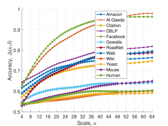
Figure 2: The accuracy $\Delta(\kappa,10\%)$ for all networks with $\delta=10\%$ edge-swaps. We cluster the networks by the accuracy of distinguishing $N_{0}$ from $N_{\delta}$ at scale $\kappa=24$:

fragile ($\Delta(24)>0.8$) Al-Qaeda; Facebook. semi-robust ($\Delta(24)\sim 0.7$) DBLP; Web; Road; Amazon; Citation. robust ($\Delta(24)<0.6$) Human; Yeast; Wiki; Mouse; Gowalla.

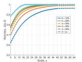
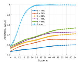
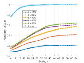
Facebook	Wiki	Human

Figure 3: Evolution of a network’s structure as it is perturbed from $\delta=10\%$ to $\infty$. A fragile network (Facebook) with intricate structure quickly becomes distinguishable with perturbation, even at small scale. A robust network (Wiki) resists the perturbations and remains somewhat indistinguishable from the original network until $\delta$ gets very large.

Recall that a high accuracy, $\Delta(\kappa)\gg{1\over 2}$, means the perturbed network at scale $\kappa$ is highly distinguishable from the original network. This means structure in the network has been disrupted. Focusing on scale $\kappa=24$ in Figure 2, we see that already at such a small scale, for some networks, there is significant distinguishability between the original network $N$ and a 10%-perturbed copy of $N$. Indeed, the networks appear to cluster into three groups which we categorize loosely as fragile ($\Delta>0.8$), semi-robust ($\Delta\sim 0.7$) and robust ($\Delta<0.6$). In the fragile networks, which are the social networks, a small perturbation destroys the local structure leading to high distinguishability. This may not be a surprise as people usually choose their friends carefully and even small perturbations will disrupt those finely tuned social circles – this is especially so in the Al-Qaeda network which achieves more than 90% distinguishability with just 10% edge-swaps. In robust networks, the distinguishability with just a 10% perturbation is only marginally above random. This does not mean there is no structure at the 24-node scale. It just means the structure has not yet been significantly disrupted by so small a perturbation. The biological networks fall into our classification of robust, which may indicate a level of redundancy/degeneracy that has been accumulated over the evolutionary process. The semi-robust networks are also interesting (DBLP, Web, Road, Amazon, Citation). These networks do have structure, but that structure is not so fragile as the social networks, indicating that the structure is not as fine tuned. Indeed, these networks have grown in an ad-hoc manner to represent the activity patterns of their actors, rather than being explicitly created by their actors (cf. social networks).

Figure 3 shows how structure gets dismantled as the perturbation increases from $\delta=10\%$ to $\delta=\infty$ for three networks: Facebook (fragile social network); Wiki (robust information network); and, a biological network. Facebook quickly yields and after 50% edge-swaps the network has more-or-less reached a random graph with the same degrees. The Wiki network, on the other hand, resists, and even after 50% edge-swaps, the network is still not significantly discernible from the original unperturbed network. The mixing time for the edge-swapping random process is much slower on the robust Wiki network. The biological network resits small perturbations but slowly yields its structure with larger perturbations.

Intrinsic Scale.

The view presented in Figure 3 highlights the evolution of a network as it is perturbed. Some networks vigorously resist even at large scales (hard to distinguish from the original network) and some fall apart even at smaller scales (easy to distinguish from the original network). We now go back to Figure 2 and focus on intrinsic scale. Figure 4 shows results analogous to Figure 2, but for increasing values of the perturbation $\delta$. The typical behavior is a rapid rise in accuracy as scale increases, which corresponds to a rapid dismantling of the networks structure. This is followed by an elbow-turning point after which diminishing returns results in a flattening. The turning point (elbow) roughly corresponds to intrinsic scale, the scale at which all the observable structure has been dismantled by the perturbation – going to larger scale does not improve accuracy significantly.

We now focus on $\delta=\infty$ to define the intrinsic scale. This choice of $\delta$ is to capture all the structure, whether fragile or robust – we must perturb hard enough to overcome the “robustness” of the network. For small perturbations, inability to distinguish the perturbed from the non-perturbed subgraphs may not indicate a lack of structure, but just that whatever structure exists may not yet have been dismantled. At $\delta=\infty$, all existing structure beyond the vertex degrees is gone. Indistinguishability now means there was no structure to start with. Distinguishability with high accuracy says that there was enough structure at the beginning. This structure may have been fragile or robust, but at $\delta=\infty$ we can’t tell.

Visually looking at the elbows in Figure 4 for $\delta=\infty$ suggests that the networks roughly cluster into three categories.

Highly Structured Road. (no surprise)

Semi-structured Al-Qaeda, DBLP; Web; Road; Amazon; Citation; Gowalla.

Loosely structured Wiki; Yeast; Mouse; Human.

Computing the elbow in the curves is not well defined and hard to generalize, so we opt for a simpler definition of intrinsic scale: the accuracy at $\delta=\infty$ must be above 95%. This accuracy threshold is quite strict and an intrinsic scale defined by the elbow will usually be smaller. Nevertheless, we opt for this simpler and more conservative definition. The intrinsic scales presented in Table 1 for different accuracy thresholds can all be obtained from Figure 4. The surprising conclusion is that for all these networks, spanning a variety of domains, the intrinsic scale is no more than 20 and as low as 7.

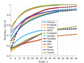
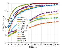
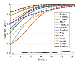
(a) $\delta=30\%$	(b) $\delta=50\%$	(c) $\delta=\infty$

Figure 4: Intrinsic scale at different levels of perturbation $\delta$. All networks display a “rapid” rise in accuracy (structure is rapidly lost) followed by an elbow followed by a flattening. As a sanity check, we also show the accuracy for an Erdős-Renyi random graph at different scales for $\delta=\infty$. Such a graph has no “structure” at any scale, and it is no surprise that the accuracy hovers around ${1\over 2}$ for all scales.

It is also interesting to note from Figure 4(c) that the accuracy approaches but doesn’t quite reach 1. This asymptotic gap away from $1$ indicates an amount of randomness in the original graph that cannot be distinguished from the random graph. This gap has about a 0.7 correlation with the intrinsic scale, and ranges from $0.17\%$ for the Road network to about $0.58\%$ for the Wiki network.

Feature-Based Classification.

Our algorithm to estimate $\Delta(\kappa,\delta)$ uses a learned classifier, and we have focused on the CNN with graph-images from (Wu et al., 2016; Hegde et al., 2018). We briefly compare with more traditional feature-based methods. As a point of comparison, we take the Facebook network with $\delta=\infty$, and consider two classical features:

Clustering coefficient, $$C r$$: Average fraction of closed triangles per vertex. Measure of Assortativity, : Average neighbor degree.

We show histograms of these features for 8-node subgraphs of the Facebook network and its perturbation in Figure 5.

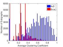
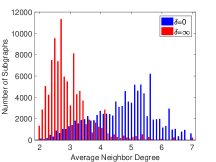
Figure 5: Classical features: histograms of clustering coefficient (fraction of closed triangles) and assortativity (average neighbor degree) for 8-node subgraphs of the Facebook network with $\delta=0$ and $\delta=\infty$. The perturbed and non-perturbed subgraphs induce distinguishable distributions over these features.

The distributions $p_{8,0}$ and $p_{8,\infty}$ are clearly distinguishable. We can compute the Bayes optimal accuracy for each feature using [2] where the sum over graphs $G$ is replaced by a sum of the feature’s values. The results are in the table below.

Classifier $$\hat{\Delta}(8,\infty) C r C r +$$ Bayes optimal using 0.905 Bayes optimal using 0.820 Bayes optimal using and 0.932 CNN graph-image 0.934

The CNN with the graph-image gives the best (highest) estimate $\hat{\Delta}$. Naturally, we can try other features and combinations of them, but one cannot exhaust all the possibilities for any given network, and further, a feature that works well for one type of network may not work well for another. And even still, there is no guarantee that the optimal estimate from using the features is better than the CNN plus graph-image. The graph-image feature is general, lossless and agnostic to the size and type of the network and when combined with the CNN gives top performance. Therefore CNN $+$ graph-image was an easy choice for our classification problem.

Other Measures of Scale.

Our intrinsic scale is not correlated with network-size (the correlations are negative: $-0.6$ with —V—, and $-0.3$ with —E—). We compare our measure of intrinsic scale with other reasonable measures of scale:

Cluster size: Average of the cluster-sizes from the Speakeasy algorithm in (Gaiteri et al., 2015). 1-neighborhood size: Also the average degree, $$2|E|/|V|$$. Shortest path-length: Average over a large number of randomly sampled pairs of nodes. Network diameter: A measure of global scale.

We compare our intrinsic scale with these measures below.

Network Intrinsic scale Cluster Size Neigh. Size Av. path length Diameter Road 7 5.95 2.83 308.91 753 Facebook 10 82.42 43.7 3.83 7 Human 10 12.26 6.46 4.25 7 Amazon 12 10.88 5.53 11.97 31 Al-Qaeda 12 8.47 5.58 3.5 4 Cite 12 48.45 24.4 4.36 10 DBLP 13 9.77 6.62 6.79 15 Web 14 19.08 11.7 6.34 16 Gowalla 17 17.65 9.67 4.62 11 Mouse 20 7.68 2.86 4.86 10 Yeast 20 18.56 16.9 3.28 6 Wiki 20 199.65 52.1 2.55 4 corr. coef. 1.000 0.3266 0.2257 -0.5047 -0.5043

We also show the correlation coefficient of the other measures with intrinsic scale. None of the other measures are highly correlated with intrinsic scale. The closest is cluster size which can be much larger and dependent on the clustering algorithm. Intrinsic scale captures something non-trivial.

Conclusion

Our methodology for extracting the intrinsic scale of a network poses the task as a classification problem. This classification problem is to distinguish subgraphs on the network from subgraphs on a perturbed copy of the network. The accuracy $\Delta(\kappa,\delta)$ quantifies how much structure in the network at scale $\kappa$ gets dismantled by a $\delta$-perturbation. The learning curves for a fixed scale $\kappa$ in Figure 6 show how the accuracy at that scale increases as one dismantles the structure in the network (by increasing $\delta$). The rate at which structure gets dismantled for small perturbations is related to the robustness of the network, which we denote $\gamma$:

$$\text{robustness, $\gamma(\kappa)$}=-\ln(\Delta(\kappa,10\%)-{\textstyle 0.5}).$$

(logarithm(inverse of uplift in accuracy over random) for 10% perturbation). Robust networks hold on to their structure for small perturbations.

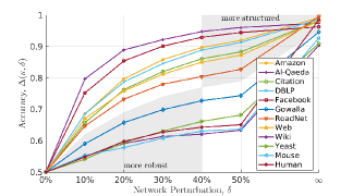
Figure 6: Learning curves for $\kappa=16$. Small perturbations reveal a network’s robustness. Large perturbations, in particular $\delta=\infty$, reveal structure.

For large perturbations, all the structure gets dismantled and the Bayes optimal accuracy quantifies the amount of structure there was in the network to start with, irrespective of robustness. We defined the intrinsic scale $\kappa^{*}$ as the scale at which there is enough structure to achieve a classification accuracy exceeding 95%. A small intrinsic scale means the network is very structured.

We summarize our findings in the following graphic which represents the networks in our study on a two-dimensional landscape of robustness and intrinsic scale.

The social networks are especially fragile, and the biological networks are especially robust. One can approximately quantify the resilience of a network’s functioning to vertex and edge removals using the degree-based parameter (see (Gao et al., 2016)):

$$\beta={\text{average squared degree}\over\text{average degree}}.$$

There is a moderate correlation of 37% between this measure of resilience $\beta$ and our measure of robustness $\gamma$. A correlation of 37% indicates some relationship between a network’s ability to maintain its function under perturbation and the statistical recognizability of a networks topology against a null distribution obtained from a small (10%) perturbation. The relationship between statistical distinguishibility and resilience may warrant further study (akin to the relationship between statistical information and algorithmic compressability of sequences).

For the networks we examined, there is about a 61% correlation between structure and robustness. More structured networks with smaller intrinsic scale tend to be less robust. Our study provides a methodology for further investigation of this structure-robustness trade-off in networks. The trade-off is by no means universal: a notable exception is the Human PPI network which is very robust and yet very structured.

Interesting future directions are: (i) Using statistical distinguishability, one can construct a taxonomy of real networks and random models with respect to the structure-robustness trade-off. One might then identify which models are appropriate for different real networks. (ii) How do we construct networks which break the structure-robustness trade-off, especially having very small intrinsic scale but very high robustness (e.g. Human PPI network). Such networks could have important applications. (iii) One can use knowledge about the intrinsic scale of a network to inform other network analysis algorithms such as clustering. For example, clusters should be defined with respect to information available within the intrinsic scale of the nodes participating in the cluster. The intrinsic scale can also guide the choice of hyperparameters in clustering algorithms which set bounds for cluster sizes, etc. Since the intrinsic scales of real networks are small, algorithmic analysis of such networks, when confined to scales on the order of the intrinsic scale, should be more efficient.

References

- Baumes et al. (2005a) Baumes, J., Goldberg, M., Krishnamoorthy, M., Magdon-Ismail, M., and Preston, N. Finding communities by clustering a graph into overlapping subgraphs. In Proc. Int. Conf. on Appl. Comp. (IADIS), pp. 97–104, Portugal, February 2005a.
- Baumes et al. (2005b) Baumes, J., Goldberg, M., and Magdon-Ismail, M. Efficient identification of overlapping communities. In IEEE International Conference on Intelligence and Security Informatics (ISI), pp. 27–36, Atlanta, Georgia, May, 19-20 2005b.
- Cho et al. (2011) Cho, E., Myers, S. A., and Leskovec, J. Friendship and mobility: user movement in location-based social networks. KDD, 2011.
- Fortunato (2010) Fortunato, S. Community detection in graphs. Physics Reports, 486(3):75 – 174, 2010.
- Gaiteri et al. (2015) Gaiteri, C., Chen, M., Szymanski, B., Kuzmin, K., Xie, J., Lee, C., Blanche, T., Neto, E. C., Huang, S.-C., Grabowski, T., et al. Identifying robust communities and multi-community nodes by combining top-down and bottom-up approaches to clustering. Scientific Reports, 5:16361, 2015.
- Gao et al. (2016) Gao, J., Barzel, B., and Barabasi, A.-L. Universal resilience patterns in complex networks. Nature, 530(7590):307–312, 2016.
- Gehrke et al. (2003) Gehrke, J., Ginsparg, P., and Kleinberg, J. Overview of the 2003 KDD cup. SIGKDD Newsl., 2003.
- Hagberg et al. (2008) Hagberg, A. A., Schult, D. A., and Swart, P. J. Exploring network structure, dynamics, and function using NetworkX. Proceedings of the 7th Python in Science Conference (SciPy2008), 2008.
- Hegde et al. (2018) Hegde, K., Magdon-Ismail, M., Ramanathan, R., and Thapa, B. Network signatures from image representation of adjacency matrices: Deep/transfer learning for subgraph classification. arXiv:1804.06275, 2018.
- JJATT (2009) JJATT. John jay & artis transnational terrorism database, 2009. URL http://doitapps.jjay.cuny.edu/jjatt/data.php.
- Leskovec & Mcauley (2012) Leskovec, J. and Mcauley, J. J. Learning to discover social circles in ego networks. NIPS, 2012.
- Leskovec et al. (2005) Leskovec, J., Kleinberg, J., and Faloutsos, C. Graphs over time: Densification laws, shrinking diameters and possible explanations. KDD, 2005.
- Leskovec et al. (2007) Leskovec, J., Adamic, L. A., and Huberman, B. A. The dynamics of viral marketing. TWEB, 2007.
- Leskovec et al. (2009) Leskovec, J., Lang, K. J., Dasgupta, A., and Mahoney, M. W. Community structure in large networks: Natural cluster sizes and the absence of large well-defined clusters. Internet Math., 2009.
- Mukherjee & Speed (2008) Mukherjee, S. and Speed, T. P. Network inference using informative priors. Proceedings of the National Academy of Sciences, 105(38):14313–14318, 2008.
- Newman (2006) Newman, M. E. J. Modularity and community structure in networks. Proceedings of the National Academy of Sciences, 103(23):8577–8582, 2006. ISSN 0027-8424. doi: 10.1073/pnas.0601602103. URL http://www.pnas.org/content/103/23/8577.
- Newman & Girvan (2004) Newman, M. E. J. and Girvan, M. Finding and evaluating community structure in networks. Phys. Rev. E, 69:026113, 2004. doi: 10.1103/PhysRevE.69.026113. URL https://link.aps.org/doi/10.1103/PhysRevE.69.026113.
- Olbrich et al. (2010) Olbrich, E., Kahle, T., Bertschinger, N., Ay, N., and Jost, J. Quantifying structure in networks. The European Physical Journal B, 2010.
- Reagans & McEvily (2003) Reagans, R. and McEvily, B. Network structure and knowledge transfer: The effects of cohesion and range. Administrative Science Quarterly, 48(2):240–267, 2003. doi: 10.2307/3556658. URL https://doi.org/10.2307/3556658.
- Reimand et al. (2008) Reimand, J., Tooming, L., Peterson, H., Adler, P., and Vilo, J. Graphweb: mining heterogeneous biological networks for gene modules with functional significance. Nucleic acids research, 36(suppl_2):W452–W459, 2008.
- Seidman (1983) Seidman, S. B. Network structure and minimum degree. Social Networks, 1983.
- Tononi et al. (1999) Tononi, G., Sporns, O., and Edelman, G. M. Measures of degeneracy and redundancy in biological networks. Proceedings of the National Academy of Sciences, 96(6):3257–3262, 1999.
- West & Leskovec (2012) West, R. and Leskovec, J. Human wayfinding in information networks. WWW, 2012.
- West et al. (2009) West, R., Pineau, J., and Precup, D. Wikispeedia: An online game for inferring semantic distances between concepts. IJCAI, 2009.
- Wu et al. (2016) Wu, K., Watters, P., and Magdon-Ismail, M. Network classification using adjacency matrix embeddings and deep learning. ASONAM, 2016.
- Yang & Leskovec (2012) Yang, J. and Leskovec, J. Defining and evaluating network communities based on ground-truth. ICDM, 2012.