Sundial: Using Sunlight to Reconstruct Global Timestamps

Abstract

This paper investigates postmortem timestamp reconstruction in environmental monitoring networks. In the absence of a time-synchronization protocol, these networks use multiple pairs of (local, global) timestamps to retroactively estimate the motes’ clock drift and offset and thus reconstruct the measurement time series. We present Sundial, a novel offline algorithm for reconstructing global timestamps that is robust to unreliable global clock sources. Sundial reconstructs timestamps by correlating annual solar patterns with measurements provided by the motes’ inexpensive light sensors. The surprising ability to accurately estimate the length of day using light intensity measurements enables Sundial to be robust to arbitrary mote clock restarts. Experimental results, based on multiple environmental network deployments spanning a period of over 2.5 years, show that Sundial achieves accuracy as high as 10 parts per million (ppm), using solar radiation readings recorded at 20 minute intervals.

1 Introduction

A number of environmental monitoring applications have demonstrated the ability to capture environmental data at scientifically-relevant spatial and temporal scales [11, 12]. These applications do not need online clock synchronization and in the interest of simplicity and efficiency often do not employ one. Indeed, motes do not keep any global time information, but instead, use their local clocks to generate local timestamps for their measurements. Then, a postmortem timestamp reconstruction algorithm retroactively uses (local, global) timestamp pairs, recorded for each mote throughout the deployment, to reconstruct global timestamps for all the recorded local timestamps. This scheme relies on the assumptions that a mote’s local clock increases monotonically and the global clock source (e.g., the base-station’s clock) is completely reliable. However, we have encountered multiple cases in which these assumptions are violated. Motes often reboot due to electrical shorts caused by harsh environments and their clocks restart. Furthermore, basestations’ clocks can be desynchronized due to human and other errors. Finally the basestation might fail while the network continues to collect data.

We present Sundial, a robust offline time reconstruction mechanism that operates in the absence of any global clock source and tolerates random mote clock restarts. Sundial’s main contribution is a novel approach to reconstruct the global timestamps using only the repeated occurrences of day, night and noon. We expect Sundial to work alongside existing postmortem timestamp reconstruction algorithms, in situations where the basestations’ clock becomes inaccurate, motes disconnect from the network, or the basestation fails entirely. While these situations are infrequent, we have observed them in practice and therefore warrant a solution. We evaluate Sundial using data from two long-term environmental monitoring deployments. Our results show that Sundial reconstructs timestamps with an accuracy of one minute for deployments that are well over a year.

2 Problem Description

Figure 1: An illustration of mote reboots, indicated by clock resets. Arrows indicate the segments for which anchor points are collected.

The problem of reconstructing global timestamps from local timestamps applies to a wide range of sensor network applications that correlate data from different motes and external data sources. This problem is related to mote clock synchronization, in which motes’ clocks are persistently synchronized to a global clock source. However, In this work, we focus on environmental monitoring applications that do not use online time synchronization, but rather employ postmortem timestamp reconstruction to recover global timestamps.

2.1 Recovering Global Timestamps

As mentioned before, each mote records measurements using its local clock which is not synchronized to a global time source. During the lifetime of a mote, a basestation equipped with a global clock collects multiple pairs of (local, global) timestamps. We refer to these pairs as anchor points. Furthermore, we refer to the series of local timestamps as $LTS$ and the series of global timestamps as $GTS$. The basestation maintains a list of anchor points for each mote and is responsible for reconstructing the global timestamps using the anchor points and the local timestamps.

The mapping between local clock and global clock can be described by the linear relation $GTS=\alpha\cdot LTS+\beta$, where $\alpha$ represents the slope and $\beta$ represents the intercept (start time). The basestation computes the correct $\alpha$ and $\beta$ for each mote using the anchor points. Note that these $\alpha$ and $\beta$ values hold, if and only if the mote does not reboot. In the subsections that follow, we describe the challenges encountered in real deployments where the estimation of $\alpha$ and $\beta$ becomes non-trivial.

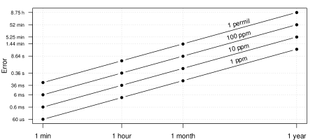
Figure 2: Time reconstruction error due to $\alpha$ estimation errors as a function of the deployment lifetime.

2.2 Problems in Timestamp Reconstruction

The methodology sketched in Section 2.1 reconstructs the timestamps for blocks of measurements where the local clock increase monotonically. We refer to such blocks as segments. Under ideal conditions, a single segment includes all the mote’s measurements. However, software faults and electrical shorts (caused by moisture in the mote enclosures) are two common causes for unattended mote reboots. The mote’s local clock resets after a reboot and when this happens we say that the mote has started a new segment.

When a new segment starts, $\alpha$ and $\beta$ must be recomputed. This implies that the reconstruction mechanism described above must obtain at least two anchor points for each segment. However, as node reboots can happen at arbitrary times, collecting two anchor points per segment is not always possible. Figure 1 shows an example where no anchor points are taken for the biggest segment, making the reconstruction of timestamps for that segment problematic. In some cases we found that nodes rebooted repeatedly and did not come back up immediately. Having a reboot counter helps recover the segment chronology but does not provide the precise start time of the new segment.

Furthermore, the basestation is responsible for providing the global timestamps used in the anchor points. Our experience shows that assuming the veracity of the basestation clock can be precarious. Inaccurate basestation clocks can corrupt anchor points and lead to bad estimates of $\alpha$ and $\beta$ introducing errors in timestamp reconstruction. Long deployment exacerbate these problems, as Figure 2 illustrates: an $\alpha$ error of 100 parts per million (ppm) can lead to a reconstruction error of 52 minutes over the course of a year.

2.3 A Test Case

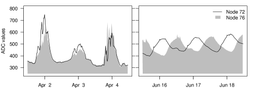
Figure 3: Ambient temperature data from two motes from the L deployment. The correlation of temperature readings in the left panel indicates consistent timestamps at the segment’s start. After two months, the mote’s reading become inconsistent due to inaccurate $\alpha$ estimates.

Our Leakin Park deployment (referred to as “L”) provides an interesting case study of the problems described above. The L deployment comprised six motes deployed in an urban forest to study the spatial and temporal heterogeneity in a typical urban soil ecosystem. The deployment spanned over a year and a half, providing us with half a million measurements from five sensing modalities. We downloaded data from the sensor nodes very infrequently using a laptop PC and collected anchor points only during these downloads. One of the soil scientists in our group discovered that the ambient temperature values did not correlate among the different motes. Furthermore, correlating the ambient temperature with an independent weather station, we found that the reconstruction of timestamps had a major error in it.

Figure 3 shows data from two ambient temperature sensors that were part of the L deployment. Node 72 and 76 show coherence for the period in April, but data from June are completely out-of-sync. We traced the problem back to the laptop acting as the global clock source. We made the mistake of not synchronizing its clock using NTP before going to the field to download the data. As a result the laptop’s clock was off by 10 hours, giving rise to large errors in our $\alpha$ and $\beta$ estimates and thereby introducing large errors in the reconstructed timestamps. To complicate matters further, we discovered that some of the motes had rebooted a few times between two consecutive downloads and we did not have any anchor points for those segments of data.

Algorithm 1 Robust Global Timestamp Reconstruction (RGTR)

constants

$Q$ $\triangleright$ Constant used to identify anchor points for the segment

$\delta_{HIGH},\ \delta_{LOW},\ \delta_{DEC}$ $\triangleright$ Constants used in iterative fit

procedure ClockFit($ap$)

    $(r,i)\leftarrow(0,0)$

    $q\leftarrow$ HoughQuantize($ap$)

    for each $\gamma$ in Keys($q$) do

       $s\leftarrow$ Size($q\{\gamma\}$)

       if $s>r$ then

          $(r,i)\leftarrow(s,\gamma)$            

    return ComputeAlphaBeta($q\{i\}$)

procedure HoughQuantize($ap$)

    $q\leftarrow\{\}$ $\triangleright$ Map of empty sets

    for each $(lts_{i},gts_{i})$ in $ap$ do

       for each $(lts_{j},gts_{j})$ in $ap$ and $(lts_{j},gts_{j})\neq(lts_{i},gts_{i})$ do

          $\alpha\leftarrow(gts_{j}-gts_{i})/(lts_{j}-lts_{i})$

          if $0.9\leq\alpha\leq 1.1$ then $\triangleright$ Check if part of the same segment

             $\beta\leftarrow gts_{j}-\alpha\cdot lts_{j}$

             $\gamma\leftarrow ROUND(\beta/Q)$

             Insert($q\{\gamma\},(lts_{i},gts_{i})$)

             Insert($q\{\gamma\},(lts_{j},gts_{j})$)                      

    return $q$

procedure ComputeAlphaBeta($ap$)

    $\delta\leftarrow\delta_{HIGH}$

    $bad\leftarrow\{\}$

    while $\delta>\delta_{LOW}$ do

       $(\alpha,\beta)\leftarrow$ LLSE($ap$)

       for each $(lts,gts)\in ap$ and $(lts,gts)\notin bad$ do

          $residual\leftarrow(\alpha\cdot lts+\beta)-gts$

          if $residual\geq|\delta|$ then

             Insert($bad,(lts,gts)$)                  

       $\delta\leftarrow\delta-\delta_{DEC}$     

    return $(\alpha,\beta$)

3 Solution

The test case above served as the motivation for a novel methodology that robustly reconstructs global timestamps. The Robust Global Timestamp Reconstruction (RGTR) algorithm, presented in Section 3.1, outlines a procedure to obtain robust estimates of $\alpha$ and $\beta$ using anchor points that are potentially unreliable. We address situations in which the basestation fails to collect any anchor points for a segment through a novel method that uses solar information alone to generate anchor points. We refer to this mechanism as Sundial.

3.1 Robust Global Timestamp Reconstruction (RGTR)

Having a large number of anchor points ensures immunity from inaccurate ones, provided they are detected. Algorithm 1 describes the Robust Global Timestamp Reconstruction (RGTR) algorithm that achieves this goal. RGTR takes as input a set of anchor points ($ap$) for a given segment and identifies the anchor points that belong to that segment, while censoring the bad ones. Finally, the algorithm returns the $(\alpha,\beta)$ values for the segment. RGTR assumes the availability of two procedures: Insert and Llse. The Insert$(x,y)$ procedure adds a new element, $y$, to the set $x$. The Linear Least Square Estimation [4], Llse procedure takes as input a set of anchor points belonging to the same segment and outputs the parameters $(\alpha,\beta)$ that minimize the sum of square errors.

RGTR begins by identifying the anchor points for the segment. The procedure HoughQuantize implements a well known feature extraction method, known as the Hough Transform [5]. The central idea of this method is that anchor points that belong to the same segment should fall on a straight line having a slope of $\sim 1.0$. Also, if we consider pairs of anchors (two at a time) and quantize the intercepts, anchors belonging to the same segment should all collapse to the same quantized value (bin). HoughQuantize returns a map, $q$, which stores the anchor points that collapse to the same quantized value. The key (stored in $i$) that contains the maximum number of elements contains the anchor points for the segment.

Figure 4: The solar (model) length of day (LOD) and noon pattern for a period of two years for the latitude of our deployments.

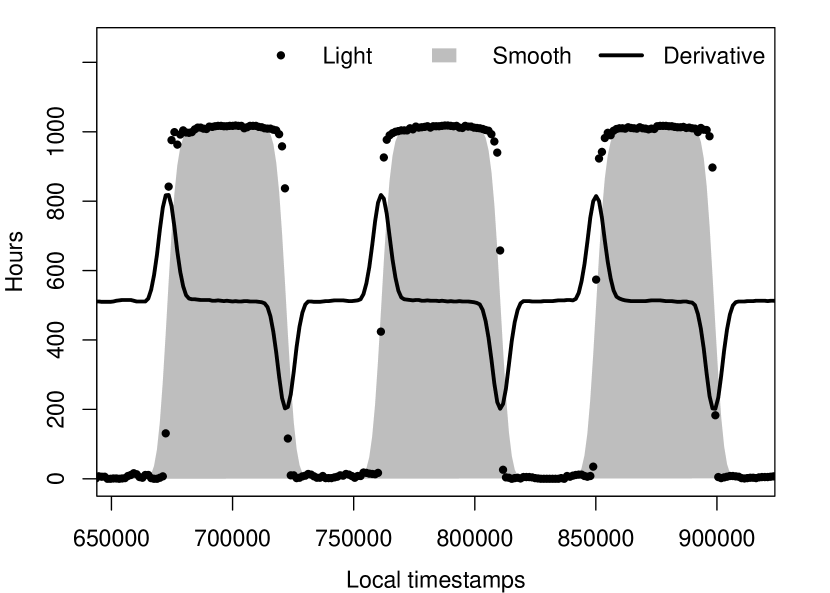
Figure 5: The light time series (raw and smoothed) and its first derivative. The inflection points represent sunrise and sunset.

Next, we invoke the procedure ComputeAlphaBeta to compute robust estimates of $\alpha$ and $\beta$ for a given segment. We begin by creating an empty set, $bad$. The set $bad$ maintains a list of all anchor points that are detected as being outliers and do not participate in the parameter estimation. This procedure is iterative and begins by estimating the fit ($\alpha,\beta$) using all the anchor points. Next, we look at the residual of all anchor points with the fit. Anchor points whose residuals exceed the current threshold, $\delta$, are added to the $bad$ set and are excluded in the next iteration fit. Initially, $\delta$ is set conservatively to $\delta_{HIGH}$. At the end of every iteration, the $\delta$ threshold is lowered and the process repeats until no new entries are added to the $bad$ set, or $\delta$ reaches $\delta_{LOW}$.

3.2 Sundial

The parameters of the solar cycle (sunrise, sunset, noon) follow a well defined pattern for locations on Earth with a given latitude. This pattern is evident in Figure 5 that presents the length of day (LOD) and solar noon for the period between January 2006 and June 2008 for the latitude of the L deployment. Note that the LOD signal is periodic and sinusoidal. Furthermore, the frequency of the solar noon signal is twice the frequency of the LOD signal. We refer the reader to [6] for more details on how the length of day can be computed for a given location and day of the year.

The paragraphs that follow explain how information extracted from our light sensors can be correlated with known solar information to reconstruct the measurement timestamps.

Figure 6: The length of day pattern for two long segments belonging to different nodes. Day 0 represents the start-time for each of the segments.

3.2.1 Extracting light patterns:

We begin by looking at the time series $L_{i}$ of light sensor readings for node $i$. $L_{i}$ is defined for a single segment in terms of the local clock. First, we create a smooth version of this series, to remove noise and sharp transients. Then, we compute the first derivative for the smoothed $L_{i}$ series, generating the $D_{i}$ time-series. Figure 5 provides an illustration of a typical $D_{i}$ series overlaid on the light sensor series ($L_{i}$). One can notice the pattern of inflection points representing sunrise and sunset. The regions where the derivative is high represent mornings, while the regions where the derivative is low represent evenings. For this method, we select sunrise to be the point at which the derivative is maximum and sunset the point at which the derivative is minimum. Then, LOD is given as the difference between sunrise and sunset, while noon is set to the midpoint between sunrise and sunset.

The method described above accurately detects noon time. However, the method introduces a constant offset in LOD detection and it underestimates LOD due to a late sunrise detection and an early sunset detection. The noon time is unaffected due to these equal but opposite biases. In practice, we found that a simple thresholding scheme works best for finding the sunrise and sunset times. The light sensors’ sensitivity to changes simplifies the process of selecting the appropriate threshold. In the end, we used a hybrid approach whereby we obtain noon times from the method that uses derivatives and LOD times from the thresholding method. The net result of this procedure is a set of noon times and LOD for each day from the segment’s start in terms of the local clock. Figure 6 shows the LOD values obtained for two different node segments after extracting the light patterns.

Figure 7: An illustration of the computed LOD and noon values for the lag with maximum correlation with the solar model.

3.2.2 Solar reconstruction of clocks:

The solar model provides the LOD and noon values in terms of the global clock ($LOD_{GT}$), while the procedure described in the previous paragraph extracts the LOD and noon values from light sensor measurements in terms of the motes’ local clocks ($LOD_{LT}$). In order to find the best possible day alignment, we look at the correlation between the two LOD signals ($LOD_{GT},LOD_{LT}$) as a function of the lag (shift in days). The lag that gives us the maximum correlation ($\rho_{max}$) is an estimate of the day alignment. Mathematically, the day alignment estimate (lag) is obtained as

$$\arg\max_{lag}\text{Cor}(LOD_{GT},LOD_{LT},lag)$$

where $\text{Cor}(X,Y,s)$ is the correlation between time series $X$ and $Y$ shifted by $s$ time units. Figure 7 presents an example of the match between model and computed LOD and noon times achieved by the lag with the highest correlation. The computed LOD time series tracks the one given by the solar model. One also observes a constant shift between the two LOD patterns, which can be attributed to the horizon effect. For some days, canopy cover and weather patterns cause the extracted LOD to be underestimated. However, as the day alignment is obtained by performing a cross-correlation with the model LOD pattern, the result is robust to constant shifts. Furthermore, Figure 7 shows that the equal and opposite effect of sunrise and sunset detection ensures that the noon estimation in unaffected in the average case.

After obtaining the day alignment, we use the noon information to generate anchor points. Specifically, for each day of the segment we have available to us the noon time in local clock (from the light sensors) and noon time in global clock (using the model). RGTR can then be used to obtain robust values of $\alpha$ and $\beta$. This fit is used to reconstruct the global timestamps. As Figure 5 suggests, the noon times change slowly over consecutive days as they oscillate around 12:00. Thus, even if the day estimate is inaccurate, due to the small difference in noon times, the $\alpha$ estimate remains largely unaffected. This implies that even if the day alignment is not optimal, the time reconstruction within the day will be accurate, provided that the noon times are accurately aligned. The result of an inaccurate lag estimate is that $\beta$ is off by a value equal to the difference between the actual day and our estimate. In other words, $\beta$ is off by an integral and constant number of days (without any skew) over the course of the whole deployment period.

Figure 8: The steps involved in reconstructing global timestamps using Sundial.

We find that this methodology is well suited in finding the correct $\alpha$. To improve the $\beta$ estimate, we perform an iterative procedure which works as follows. For each iteration, we obtain the best estimate fit ($\alpha,\beta$). We convert the motes’ local timestamps into global timestamps using this fit. We then look at the difference between the actual LOD (given by the model) and the current estimate for that day. If the difference between the expected LOD and the estimate LOD exceeds a threshold, we label that day as an outlier. We remove these outliers and perform the LOD cross-correlation to obtain the day shift (lag) again. If the new lag differs from the lag in the previous iteration, a new fit is obtained by shifting the noon times by an amount proportional to the new lag. We iterate until the lag does not change from the previous iteration. Figure 8 shows a schematic of the steps involved in reconstructing global timestamps for a segment.

Figure 9: Node identifiers, segments and length of each segment (in days) for the two deployments used in the evaluation.

4 Evaluation

We evaluate the proposed methodology using data from two deployments. Deployment J was done at the Jug Bay wetlands sanctuary along the Patuxent river in Anne Arundel County, Maryland. The data it collected is used to study the nesting conditions of the Eastern Box turtle (Terrapene carolina) [10]. Each of the motes was deployed next to a turtle nest, whereas some of them have a clear view of the sky while others are under multiple layers of tree canopy. Deployment L, from Leakin Park, is described in Section 2.3.

Figure 9 summarizes the node identifiers, segments, and segment lengths in days for each of the two deployments. Recall that a segment is defined as a block of data for which the mote’s clock increases monotonically. Data obtained from the L dataset contained some segments lasting well over 500 days. The L deployment uses MicaZ motes [3], while the J deployment uses TelosB motes [8]. Motes 2, 5, and 6 from Deployment J collected samples every 10 minutes. All other motes for both deployments had a sampling interval of 20 minutes. In addition to its on-board light, temperature, and humidity sensors, each mote was connected to two soil moisture and two soil temperature sensors.

In order to evaluate Sundial’s accuracy, we must compare the reconstructed global timestamps it produces, with timestamps that are known to be accurate and precise. Thus we begin our evaluation by establishing the ground truth.

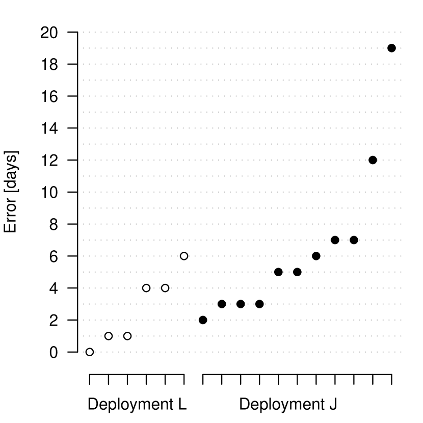
Figure 10: Error in days for different motes from the L and J deployments.

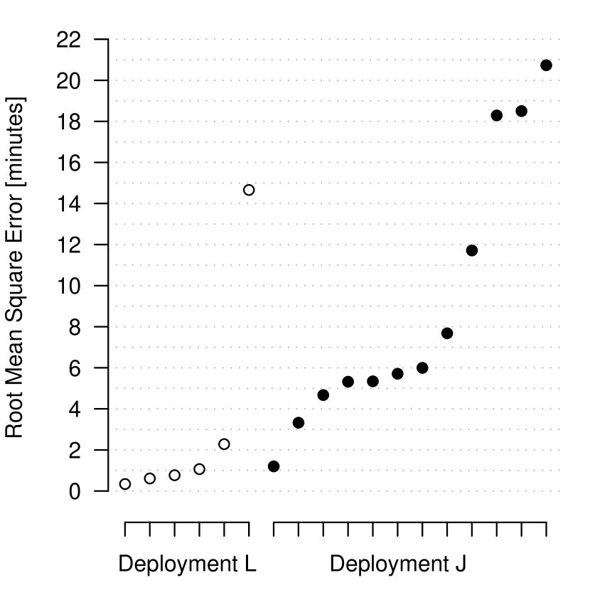
Figure 11: Root mean square error in minutes $(RMSE_{min})$.

4.1 Ground Truth

For each of the segments shown in Figure 9, a set of good anchor points (sampled using the basestation) were used to obtain a fit that maps the local timestamps to the global timestamps. We refer to this fit as the Ground truth fit. This fit was validated in two ways. First, we correlated the ambient temperature readings among different sensors. We also correlated the motes’ measurements with the air temperature measurements recorded by nearby weather stations. The weather station for the L deployment was located approximately 17 km away from the deployment site [1], while the one for the J deployment was located less than one km away [7]. Considering the proximity of the two weather stations we expect that their readings are strongly correlated to the motes’ measurements.

Note that even if the absolute temperature measurements differ, the diurnal temperature patterns should exhibit the same behavior thus leading to high correlation values. Visual inspection of the temperature data confirmed this intuition. Finally, we note that due to the large length of the segments we consider, any inconsistencies in the ground truth fit would become apparent for reasons similar to the ones provided in Section 2.2.

Figure 12: Relation between $\rho_{max}$ and error in days.

Figure 13: $\alpha$ estimates from Sundial and estimation errors in ppm.

4.2 Reconstructing Global Timestamps using Sundial

We evaluate Sundial using data from the segments shown in Figure 9. Specifically, we evaluate the accuracy of the timestamps reconstructed by Sundial as though the start time of these segment is unknown (similar to the case of a mote reboot) and no anchor points are available. Since we make no assumptions of the segment start-time, a very large model (solar) signal needs to be considered to find the correct shift (lag) for the day alignment.

4.2.1 Evaluation Metrics:

We divide the timestamp reconstruction error to: (a) error in days; and (b) error in minutes within the day. The error in minutes is computed as the root mean square error ($RMSE_{min}$) over all the measurements. We divide the reconstruction error into these two components, because this decoupling naturally reflects the accuracy of estimating the $\alpha$ and $\beta$ parameters. Specifically, if the $\alpha$ estimate were inaccurate, then, as Figure 2 suggests, the reconstruction error would grow as a function of time. In turn, this would result in a large root mean squared error in minutes within the day over all the measurements. On the other hand, a low $RMSE_{min}$ corresponds to an accurate estimate for $\alpha$. Likewise, inaccuracies in the estimation of $\beta$ would result in large error in days.

4.2.2 Results:

Figures 11 and 11 summarize Sundial’s accuracy results. Overall, we find that longer segments show a lower day error. Segments belonging to the L deployment span well over a year and the minimum day error is 0 while the maximum day error is 6. In contrast, most of the segments for deployment J are less than 6 months long and the error in days for all but two of those segments is less than one week. Figure 13 presents the relationship between the maximum correlation ($\rho_{max}$) and the day error. As $\rho_{max}$ measures how well we are able to match the LOD pattern for a node with the solar LOD pattern, it is not surprising that high correlation is generally associated with low reconstruction error. The $RMSE_{min}$ obtained for each of the segments in deployment L is very low (see Figure 11) . Remarkably, we are able to achieve an accuracy ($RMSE_{min}$) of under a minute for the majority of the nodes of the L deployment even though we are limited by our sampling frequency of 20 minutes. Moreover, $RMSE_{min}$ error is always within one sample period for all but one segment.

Interestingly, we found that the $\alpha$ values for the two deployments were significantly different. This disparity can be attributed to differences in node types and thus clock logic. Nonetheless, Sundial accurately determined $\alpha$ in both cases. Figure 13 presents the $\alpha$ values for the two deployments. We also show the error between the $\alpha$ obtained using Sundial and the $\alpha$ value obtained by fitting the good anchor points sampled by the gateway (i.e., ground truth fit). The ppm error for both the deployments is remarkably low and close to the operating error of the quartz crystal.

4.3 Impact of Segment Length

Sundial relies on matching solar patterns to the ones observed by the light sensors. The natural question to ask is: what effect does the length of segment have on the reconstruction error. We address this question by experimenting with the length of segments and observing the reconstruction error in days and $RMSE_{min}$. We selected data from three long segments from deployment L. To eliminate bias, the start of each shortened segment was chosen from a uniform random distribution. Figure 15 shows that the $RMSE_{min}$ tends to be remarkably stable even for short segments. One concludes that even for short segment lengths, Sundial estimates the clock drift ($\alpha$) accurately. Figure 15 shows the effect of segment size on day error. In general, the day error decreases as the segment size increases. Moreover, for segments less than 150 days long, the error tends to vary considerably.

Figure 14: Error in days as a function of segment size.

Figure 15: Error in minutes ($RMSE_{min}$) as a function of segment size.

4.4 Day Correction

The results so far show that 88% (15 out of 17) of the motes have a day offset of less than a week. Next, we demonstrate how global events can be used to correct for the day offset. We looked at soil moisture data from eight motes of the J deployment after obtaining the best possible timestamp reconstruction. Specifically, we correlated the motes’ soil moisture data with rainfall data to correct for the day offset. We used rainfall data from a period of 133 days, starting from December 4, 2007, during which 21 major rain events occurred. To calculate the correlation, we created weighted daily vectors for soil moisture measurements ($SM$) whose value was greater than a certain threshold and similarly rainfall vectors having a daily precipitation ($PPT$) value of greater than 4.0 cm. Next, we extracted the lag at which the cosine angle between the two vectors (cosine similarity, $\theta_{SM-PPT}$) is maximum. This method is inspired by the well-known document clustering model used in the information retrieval community [9]. Note that we computed $\theta_{SM-PPT}$ for a two-week window ($\pm$ seven days) of lags and found that seven out of the eight motes could be aligned perfectly. Figure 16 illustrates the soil moisture vectors, rainfall vectors and the associated $\theta_{SM-PPT}$ for seven lags for one of the segments. Note that $\theta_{SM-PPT}$ peaks at the correct lag of five, leading to the precise day correction. While we use soil moisture to illustrate how global events can be used to achieve macro-level clock adjustments, other modalities can also be used based on the application’s parameters.

Figure 16: An illustration of the cosine similarity ($\theta_{SM-PPT}$) values for seven different day lags between moisture and rainfall vectors. $\theta_{SM-PPT}$ peaks at the correct lag of five days, providing the correct day adjustment.

5 Related Work

This study proposes a solution to the problem of postmortem timestamp reconstruction for sensor measurements. To our knowledge, there is little previous work that addresses this problem for deployments that span a year or longer. Deployment length can be an issue because the reconstruction error monotonically increases as a function of time (cf. Sec.2.2). The timestamp reconstruction problem was first introduced by Werner-Allen et al. who provided a detailed account of the challenges they faced in synchronizing mote clocks during a 19-day deployment at an active volcano [13]. Specifically, while the system employed the FTSP protocol to synchronize the network’s motes, unexpected faults forced the authors to rely on an offline time rectification algorithm to reconstruct global timestamps.

While experiences such as the one reported in [13] provide motivation for an independent time reconstruction mechanism such as the one proposed in this paper, the problem addressed by Werner-Allen et al. is different from the one we aim to solve. Specifically, the volcano deployment had access to precise global timestamps (through a GPS receiver deployed at the site) and used linear regression to translate local timestamps to global time, once timestamp outliers were removed. While RGTR can also be used for outlier detection and timestamp reconstruction, Sundial aims to recover timestamps in situations where a reliable global clock source is not available.

Finally, Chang et. al. [2] describe their experiences with motes rebooting and resetting of logical clocks, but do not furnish any details of how they reconstructed the global timestamps when this happens.

6 Conclusion

In this paper we present Sundial, a method that uses light sensors to reconstruct global timestamps. Specifically, Sundial uses light intensity measurements, collected by the motes’ on-board sensors, to reconstruct the length of day (LOD) and noon time throughout the deployment period. It then calculates the slope and the offset by maximizing the correlation between the measurement-derived LOD series and the one provided by astronomy. Sundial operates in the absence of global clocks and allows for random node reboots. These features make Sundial very attractive for environmental monitoring networks deployed in harsh environments, where they operate disconnected over long periods of time. Furthermore, Sundial can be used as an independent verification technique along with any other time reconstruction algorithm.

Using data collected by two network deployments spanning a total of 2.5 years we show that Sundial can achieve accuracy in the order of a few minutes. Furthermore, we show that one can use other global events such as rain events to correct any day offsets that might exist. As expected, Sundial’s accuracy is closely related to the segment size. In this study, we perform only a preliminary investigation on how the length of the segment affects accuracy. An interesting research direction we would like to pursue is to study the applicability of Sundial to different deployments. Specifically, we are interested in understanding how sampling frequency, segment length, latitude and season (time of year) collectively affect reconstruction accuracy.

Sundial exploits the correlation between the well-understood solar model and the measurements obtained from inexpensive light sensors. In principle, any modality having a well-understood model can be used as a replacement for Sundial. In the absence of a model, one can exploit correlation from a trusted data source to achieve reconstruction, e.g., correlating the ambient temperature measurement between the motes with data obtained from a nearby weather station. However, we note that many modalities (such as ambient temperature) can be highly susceptible to micro-climate effects and exhibit a high degree a spatial and temporal variation. Thus, the micro-climate invariant solar model makes light a robust modality to reconstruct timestamps in the absence of any sampled anchor points.

Finally, we would like to emphasize the observation that most environmental modalities are affected by the diurnal and annual solar cycles and not by the human-created universal time. In this regard, the time base that Sundial establishes offers a more natural reference basis for environmental measurements.

References

- [1] Baltimore-Washington International airport, weather station. Available at: http://weather.marylandweather.com/cgi-bin/findweather/getForecast?query=BWI.
- [2] M. Chang, C. Cornou, K. Madsen, and P. Bonett. Lessons from the Hogthrob Deployments. In Proceedings of the Second International Workshop on Wireless Sensor Network Deployments (WiDeploy08), June 2008.
- [3] Crossbow Corporation. MICAz Specifications. Available at http://www.xbow.com/Support/Support_pdf_files/MPR-MIB_Series_Users_Manual.pdf.
- [4] R. Duda, P. Hart, and D. Stork. Pattern Classification. Wiley, 2001.
- [5] R. O. Duda and P. E. Hart. Use of the Hough transformation to detect lines and curves in pictures. Commun. ACM, 15(1):11–15, 1972.
- [6] W. C. Forsythea, E. J. Rykiel Jr., R. S. Stahla, H. Wua, and R. M. Schoolfield. A model comparison for daylength as a function of latitude and day of year. ScienceDirect, 80(1), Jan. 1994.
- [7] National Estuarine Research Reserve. Jug Bay weather station (cbmjbwq). Available at http://cdmo.baruch.sc.edu/QueryPages/anychart.cfm.
- [8] J. Polastre, R. Szewczyk, and D. Culler. Telos: Enabling Ultra-Low Power Wireless Research. In Proceedings of the Fourth International Conference on Information Processing in Sensor Networks: Special track on Platform Tools and Design Methods for Network Embedded Sensors (IPSN/SPOTS), Apr. 2005.
- [9] G. Salton, A. Wong, and C. S. Yang. A vector space model for automatic indexing. Commun. ACM, 18(11):613–620, 1975.
- [10] K. Szlavecz, A. Terzis, R. Musaloiu-E., C.-J. Liang, J. Cogan, A. Szalay, J. Gupchup, J. Klofas, L. Xia, C. Swarth, and S. Matthews. Turtle Nest Monitoring with Wireless Sensor Networks. In Proceedings of the American Geophysical Union, Fall Meeting, 2007.
- [11] A. Terzis, R. Musaloiu-E., J. Cogan, K. Szlavecz, A. Szalay, J. Gray, S. Ozer, M. Liang, J. Gupchup, and R. Burns. Wireless Sensor Networks for Soil Science. International Journal on Sensor Networks.
- [12] G. Tolle, J. Polastre, R. Szewczyk, N. Turner, K. Tu, P. Buonadonna, S. Burgess, D. Gay, W. Hong, T. Dawson, and D. Culler. A Macroscope in the Redwoods. In Proceedings of the 3rd ACM SenSys Conference, Nov. 2005.
- [13] G. Werner-Allen, K. Lorincz, J. Johnson, J. Lees, and M. Welsh. Fidelity and Yield in a Volcano Monitoring Sensor Network. In Proceedings of the 7th USENIX Symposium on Operating Systems Design and Implementation (OSDI), Nov. 2006.