Halo mass estimates from the Globular Cluster populations of 175 Low Surface Brightness Galaxies in the Fornax Cluster

Abstract

The halo masses $M_{halo}$ of low surface brightness (LSB) galaxies are critical measurements for understanding their formation processes. One promising method to estimate a galaxy’s $M_{halo}$ is to exploit the empirical scaling relation between $M_{halo}$ and the number of associated globular clusters ($N_{\mathrm{GC}}$). We use a Bayesian mixture model approach to measure $N_{\mathrm{GC}}$ for 175 LSB ($23\leq\left\langle\mu_{e,r}\right\rangle[\mathrm{mag\ arcsec}^{-2}]\leq 28$) galaxies in the Fornax cluster using the Fornax Deep Survey (FDS) data; this is the largest sample of low mass galaxies so-far analysed for this kind of study. The proximity of the Fornax cluster means that we can measure galaxies with much smaller physical sizes ($0.3\leq r_{e,r}\ [\mathrm{kpc}]\leq 9.5$) compared to previous studies of the GC systems of LSB galaxies, probing stellar masses down to $M_{*}\sim 10^{5}\mathrm{M_{\odot}}$. The sample also includes 12 ultra-diffuse galaxies (UDGs), with projected $r$-band half-light radii greater than 1.5 kpc. Our results are consistent with an extrapolation of the $M_{*}-M_{halo}$ relation predicted from abundance matching. In particular, our UDG measurements are consistent with dwarf sized halos, having typical masses between $10^{10}$ and $10^{11}\mathrm{M_{\odot}}$. Overall, our UDG sample is statistically indistinguishable from smaller LSB galaxies in the same magnitude range. We do not find any candidates likely to be as rich as some of those found in the Coma cluster. We suggest that environment might play a role in producing GC-rich LSB galaxies.

1 Introduction

Low surface brightness (LSB) galaxies are among the most common in the Universe, yet observational challenges (Disney, 1976) mean that they are also among the most mysterious. The existence of large LSB galaxies is a well known phenomenon. They were first detected several decades ago (e.g. Sandage & Binggeli, 1984; Bothun et al., 1987; Impey et al., 1988) but have received renewed interest in more recent years. However, their intrinsic properties and formation histories are still not fully understood and it is not clear whether they represent a distinct population from smaller LSB dwarf galaxies, which can form naturally in high spin halos expected from hierarchical galaxy formation models (e.g. Dalcanton et al., 1995; Jimenez et al., 1998) and from harassment of normal dwarf galaxies (Moore et al., 1998; Mastropietro et al., 2005).

An outstanding question is whether there is truly anything unique about the way in which large LSB galaxies form in comparison to their smaller counter-parts, given that they seem to share a continuous distribution of observable properties (Conselice et al., 2003; Wittmann et al., 2017; Conselice, 2018). Since van Dokkum et al. (2015) detected a surprisingly high abundance of large LSB galaxies (that they termed ultra-diffuse galaxies or UDGs) in the Coma Cluster, numerous theories have been proposed to explain their origins. Initially, van Dokkum et al. (2015) suggested they could reside in massive halos, similar in total mass to the Milky Way with a truncated star formation history. This is referred to as the “failed L$\star$” scenario, and is supported observationally by their unusually large sizes (optical effective radii $\geq 1.5$ kpc) together with their LSB ($\mu_{0}^{g}\geq\sim 23$), red colours and abundance in dense environments.

There are several possible mechanisms to explain the existence of UDGs other than the failed L$\star$ scenario. Yozin & Bekki (2015) have shown that ram-pressure stripping resulting from an early in-fall to cluster environments is sufficient to reproduce several properties of the Coma UDGs. Other authors have shown that different environmental effects like tidal heating may be enough to explain their formation (Collins et al., 2013; Carleton et al., 2018). While these models may seem to indicate that UDGs are phenomena associated preferentially with dense environments (supported observationally by van der Burg et al., 2017), it is also thought that a field population should exist (McGaugh, 1996; Di Cintio et al., 2017), plausibly arising from the high angular momentum tail of the dwarf galaxy population (Amorisco & Loeb, 2016) or from secular evolution processes such as supernovae feedback. Of course, there could be multiple formation scenarios for UDGs that combine both secular and environmentally-driven processes (Jiang et al., 2018).

The halo mass is a key parameter in distinguishing between formation models of UDGs. Typically, current models favour dwarf-sized halos with truncated star formation histories (e.g. Rong et al., 2017; Amorisco & Loeb, 2016), making them similar to normal LSB galaxies but larger. UDGs are abundant in high density environments such as in the centres of clusters (e.g. Mihos et al., 2015; Koda et al., 2015; Venhola et al., 2017) where they require a relatively high dark matter fraction in order to survive. However, it is not clear whether UDGs can form with lower mass-to-light ratios (M/L) in less dense environments such as the field (van Dokkum et al., 2018; Trujillo et al., 2018).

There have been several attempts to constrain the halo masses of UDGs with a variety of measurement techniques used, mainly focussing on UDGs in groups and clusters. Metrics include weak lensing (Sifón et al., 2018), prevalence of tidal features as a function of cluster radius (Mowla et al., 2017), comparisons of their spatial distribution with that of dwarf and massive galaxies (van der Burg et al., 2016; Román & Trujillo, 2017), richness of their globular cluster systems (Beasley & Trujillo, 2016; Amorisco et al., 2018; van Dokkum et al., 2017; Lim et al., 2018) as well as direct measurements of the velocity dispersions of stellar populations (van Dokkum et al., 2016) and globular cluster systems (Beasley et al., 2016; Toloba et al., 2018).

Globular clusters offer an interesting insight into the formation mechanisms of LSB galaxies. They are thought to form mainly in the early epochs of star formation within massive, dense giant molecular clouds that are able to survive feedback processes that might otherwise shut off star formation in their host galaxy (Hudson et al., 2014; Harris et al., 2017). The halo mass of galaxies has been shown to correlate well with both the number of associated GCs ($N_{\mathrm{GC}}$) and the total mass of their GC systems ($M_{\mathrm{GC}}$; e.g. Spitler & Forbes, 2009; Harris et al., 2013, 2017), which means measurements of either $N_{\mathrm{GC}}$ or $M_{\mathrm{GC}}$ can be used to constrain $M_{halo}$. However, Forbes et al. (2018) show that the traditional relation between $N_{\mathrm{GC}}$ and $M_{halo}$ may lose accuracy in the low $M_{halo}$ regime, perhaps because lower mass galaxies tend to have lower mass GCs without a common mean GC mass. Additionally, it has been shown that there is a correlation between the GC half-count radius and $M_{halo}$ (Forbes, 2017; Hudson & Robison, 2018).

The majority of studies of the GC populations of UDGs have up until now focussed on the Coma galaxy cluster, the most massive ($M_{\mathrm{tot}}\sim 6\times 10^{14}\mathrm{M_{\odot}}$, Hughes, 1998) galaxy cluster within 100 Mpc. In this paper we analyse exclusively galaxies in the core of the Fornax cluster. In comparison to Coma, it is around five times closer ($d\sim$20 Mpc, Blakeslee et al., 2009) but less massive ($M_{\mathrm{tot}}\sim 7\times 10^{13}M_{\odot}$, Drinkwater et al., 2001). Using the empirical relation of van der Burg et al. (2017), there are approximately 10 times less UDGs expected in Fornax than in Coma, many of which have been catalogued already (Muñoz et al., 2015; Venhola et al., 2017).

While overall we have a relatively small sample of UDGs, an advantage of working with the Fornax cluster is that cluster members have much larger projected sizes compared to the background galaxy population, so we can analyse the population of smaller LSB galaxies at the same time as the UDG population without contamination from interlopers. Indeed, much of the new literature surrounding LSB galaxies focusses on UDGs and this may be in-part due to the relative ease of distinguishing larger galaxies from background objects in group or cluster environments. A second advantage of Fornax over Coma is that GCs are brighter in apparent magnitude by $\sim$3.5 mag due to their relative proximity, meaning that we can probe further into the GC luminosity function.

We note that the relatively large number of galaxies we analyse in this study is important for at least partially overcoming systematic uncertainties involved in measuring halo masses with low numbers of tracers as made clear by Laporte et al. (2018) and the possible stochastic nature of the $M_{*}-M_{halo}$ relation at low mass (Brook et al., 2014; Errani et al., 2018).

In this work we provide constraints on the halo masses for a selection of LSB galaxies first identified by Venhola et al. (2017) using the optical Fornax Deep Survey (FDS, Iodice et al., 2016). The structure of the paper is as follows: We describe the data in $\S$2. In $\S$3 we describe the method to detect globular cluster candidates (GCCs) and infer the total number of GCs associated with our target galaxies. We provide our results in $\S$4, where we estimate the halo masses from the inferences on $N_{\mathrm{GC}}$ and $M_{\mathrm{GC}}$ using the empirical scaling relations of Harris et al. (2017). We discuss our results and provide conclusive remarks in $\S$5. We use the AB magnitude system throughout the paper, and adopt a distance of 20Mpc to the Fornax cluster.

2 Data

We use the four central 1$\times$1 degree² frames of the FDS (FDS IDs 10, 11, 12 & 16), i.e. the same region used by Venhola et al. (2017) in their by-eye classification of low surface brightness sources in the Fornax galaxy cluster. These data were obtained using the OmegaCAM (Kuijken, 2011) instrument on the 2.6m ESO VLT Survey Telescope (VST, Capaccioli et al., 2012) in the $u^{\prime}$, $g^{\prime}$, $r^{\prime}$ & $i^{\prime}$ bands. We note that Fornax GCs are unresolved in our data such that we consider them as point sources throughout the paper.

We specifically used the VSTtube-reduced FDS data (Grado et al., 2012; Capaccioli et al., 2015), which is optimised for point-source photometry but is not as deep as the data used by Venhola et al. (2017), which is reduced using a combination of the OmegaCAM pipeline and AstroWISE (McFarland et al., 2011), but with a slightly wider PSF than the VST-tube reduction because images with poor seeing were included in the stacks. We also performed additional photometric corrections to bring our photometry into the AB magnitude system as described in appendix B.

3 Methodology

In this work we target the GC populations of galaxies identified by-eye in the (Venhola et al., 2017, hereafter V17) catalogue. We split the sample into two groups: Low surface brightness galaxies (LSBGs), defined as those with $r$-band effective radii $r_{e,r}<1.5$ kpc and UDGs, defined as those with $r_{e,r}\geq 1.5$ kpc. The sources are defined as LSB because they were measured to have central surface brightness $\mu_{0}^{r}\geq 23$ by V17. We omit two UDGs (FDS11_LSB1 and FDS11_LSB17) from the sample because they are in significantly crowded locations and measuring their properties accurately would require a more sophisticated analysis.

Parameter	Constraint
mag ($g$)	14 to 19 [mag]
axrat	$\geq 0.95$
Nobject	0
Nmask	0

Table 1: ProFound measurement constraints for point source selection in the PSF modelling. axrat is the axis-ratio. Nobject is the number of pixels belonging to the segment that are touching another source. Nmask is the number of pixels belonging to the segment that are touching a masked region. See the ProFound documentation for more details of these parameters. Further criteria are discussed in the text.

Before running our detection algorithm, we subtract model galaxy profiles in each band using Imfit  (Erwin, 2015, see Appendix A). We were unable to get a stable Imfit model for three sources (FDS11_LSB16, FDS12_42, FDS12_47) because they were too faint, so we adopt the measurements of V17 (made from deeper stacks) for these sources and rely on a separate background subtraction procedure to remove the galaxy light (see $\S$3.3). We select only galaxies with measured $r$-band effective radii greater than 3$\arcsec$ ($\sim$ 0.3kpc at Fornax distance) so that we target cluster members with confidence (Sabatini et al., 2003; Davies et al., 2016).

We used the ProFound package (Robotham et al., 2018) for the source detection and photometry, with the following settings: skymesh=100 pixels ($\sim$20″), sigma=2 pixels, threshold=1.03, tolerance=1, skycut=1. All other settings were defaults. Our detection was performed exclusively on the $g$-band (the deepest) so that we could easily measure and account for our detection efficiency without considering the colours of individual sources. We note that we split the four FDS frames into $9\times 9$ subframes to ease the memory requirements for ProFound.

3.1 PSF models

We obtained point spread function (PSF) models for each band and subframe using our ProFound measurements as follows. Bright, unsaturated point sources were selected in the ProFound mag - R50 (approx. half-light radius) plane, using the selection criteria listed in table 1. Additionally we sigma-clipped the measurements in R50 (approximately flat over the magnitude range for point sources) and offset the relation by 4$\sigma$ with respect to the median to measure an upper-limit on R50 for the selection.

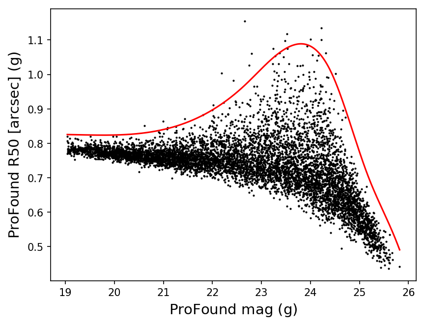
Figure 1: Point source selection function for a subframe (red line) obtained by fitting a cubic spline to measurements from the synthetic source injections (black points) after offsetting R50 by $4\sigma$ in bins of magnitude with respect to the median. All points lower than the red line are selected. The increase in scatter towards the faint end means that a simple cut in R50 would either result in a low recovery efficiency or high level of contamination from our point source selection.

We used Imfit  to fit a model Moffat profile (keeping the axis-ratio as a free parameter) to each point source following a local sky subtraction. We did not stack individual point source cut-outs to avoid artificial widening of the PSF caused by misalignment of the images. The resulting distribution of model Moffat fits was then sigma-clipped at 3$\sigma$ in the FWHM-concentration index plane to remove outliers caused by bad fits. We finally selected a fiducial model PSF for each band and subframe by adopting the fit with the average FWHM.

Of primary importance for our analysis are the $g$-band PSF models. While for a specific FDS frame we found little variation of the PSF over its subframes, on a frame-by-frame basis the Imfit FWHM ranges between approximately 0.7 and 1.2$\arcsec$.

3.2 Point source selection

We used synthetic source injections based on our Moffat PSF models from $\S$3.1 to produce our point source selection function and quantify our recovery efficiency (RE). We injected $\sim$25000 synthetic profiles per subframe into the real data at random locations in the vicinities ($420\times 420\arcsec$ cut-outs) of our target galaxies after subtracting the galaxy models from the data. This was done in the $g$-band, with apparent magnitudes ranging between 19 and 26. Our matching criteria for the synthetic sources was that the central coordinate of the injected source had to lie on top of a segment in the ProFound segmentation map. Additionally, we only considered sources that did not match with segments from the result of running ProFound over the original frames (i.e. without the injected sources). We note that the measurements of the synthetic point sources are in good agreement with measurements of real sources when plotted on the mag-R50 plane.

Once we had acquired the ProFound measurements of the synthetic sources, we fitted a smooth cubic spline to the data in the ProFound mag and R50 plane. Specifically, the spline was fit to the data binned in mag, and positively offset by 4$\sigma$ of the R50 values within the bin. See figure 1. The rationale behind this was that as sources become fainter, the scatter in R50 increases such that a simple cut at a specific value would either be too high for bright objects or conversely too low for some of the fainter objects with large values of R50. We obtained a different point source selection function for each subframe.

3.3 Colour measurement

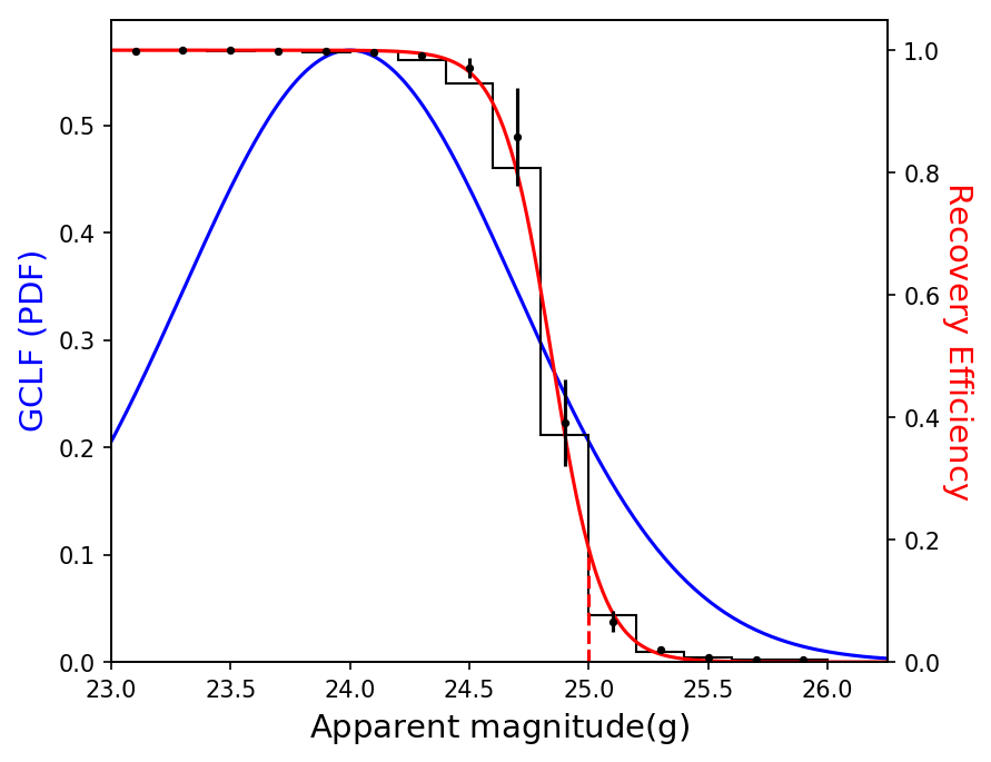
Figure 2: $g$-band recovery efficiency for a subframe of injected point sources (black histogram) after applying our selection criteria, along with the RE (red line) and a fiducial GCLF (blue line). The dashed red line shows our additional cut at $m_{g}$=25. The GCLF turnover magnitude is clearly reached by our detection pipeline. Integrating the recovery efficiency over the GCLF (including the magnitude cuts) yields an overall recovery efficiency of $\sim 80\%$. Also shown is the mean and standard deviation of the RE across all the subframes for FDS frame 10 (black errorbars).

We obtained aperture magnitudes of the ProFound sources in fixed apertures of diameter 5 pixels in all the bands. The sky level and its uncertainty were calculated for each detected source by placing many identical apertures in 51$\times$51 pixel cut-outs (the fiducial FWHM of 1$\arcsec$ is $\sim 5$ pixels) and recording the median and standard-deviation of the contained flux values after sigma clipping these at 2$\sigma$ to remove contamination from other sources. Additionally the sky apertures were placed at radii greater than 20 pixels from the centre of the source.

These magnitudes were then corrected for the PSF size in each band through calibration against an existing catalogue of PSF-corrected point sources made using the same data (Cantiello et al.; in prep.). See appendix B for a discussion of the photometric calibration procedure. We note that we have not used this catalogue for this work because of the need to subtract galaxy profiles from the data and the need to quantify the RE.

3.4 Recovery Efficiency

We quantified the RE separately for each subframe using the point source selection functions with the synthetic source measurements. We imposed a faint-end limit on the corrected $g$-band aperture magnitude of 25 mag because measuring accurate colours at fainter magnitudes is more difficult and because the degeneracy between point sources and other faint sources in the mag-R50 plane is exacerbated in this region. Additionally, we apply a lower-bound cut in the corrected $g$-band aperture magnitude of 21 mag to reduce possible contamination from bright stars, ultra-compact dwarf galaxies (UCDs) and nuclear star clusters (NSCs).

The RE itself was measured by taking the ratio of detected and selected point source injections to the total number of injected sources in bins of intrinsic magnitude. A sigmoid function,

$$\epsilon(m)=[1+\exp{(-k_{1}(k_{2}-m)})]^{-1}$$ (1)

was fit to the result (see figure 2). The recovery efficiency $\epsilon(m)$ is sufficient to reach the turnover magnitude of the $g$-band GC luminosity function (GCLF), which is approximated by a Gaussian function centred at 24$m_{g}$ at the distance of Fornax (Villegas et al., 2010). We adopt a value of 0.7 for the GCLF standard deviation, which is a reasonable estimate for low surface brightness galaxies (Trujillo et al., 2018). Under these assumptions, our estimated GC completeness ranges between $\sim$60% and 90% depending on the subframe. The mean completeness is estimated to be 82% across all the subframes. Of course, this number depends on the exact form of the adopted GCLF. While its peak at 24$m_{g}$ is fairly well known (The peak of the GCLF can sometimes be used as a standard candle, see Rejkuba, 2012), a degree of uncertainty is attributed to its width. We discuss the effects of varying the GCLF on our results in $\S$4.6.

3.5 Colour Selection

We have applied a colour selection to our point sources to produce a catalogue of globular cluster candidates (GCCs) for each target galaxy, using as few assumptions about the underlying GC colours as possible. The full colour space in $u,g,r,i$ was used for the selection. This is important because of the need to remove interloping point sources from our final GCC catalogue, which include foreground stars and unresolved background galaxies. However, we point out that both interloping populations are partially degenerate in colour space with the actual GCs (see also Pota et al., 2018) and these sources must be accounted for using spatial information (see $\S$3.6).

This colour selection was accomplished by first cross-matching our point sources from the four FDS frames with a compilation of spectroscopically confirmed Fornax compact objects (Schuberth et al., 2010; Wittmann et al., 2016; Pota et al., 2018). This resulted in a catalogue of 992 matching sources. We note that we partially account for bright UCDs with our bright-end magnitude cut-off. The external catalogue has a magnitude distribution that drops off quickly at magnitudes fainter than $\sim 23m_{g}$ and so is not complete for our purposes and this limited depth has to be accounted for.

We used the density-based clustering algorithm DBSCAN (Ester et al., 1996) to define regions in the $(u-g)-(g-r)$ and $(g-r)-(g-i)$ planes separately for our GCC selection. We used a clustering radius of 0.1 mag and required at least 5 spectroscopic GCs within this radius for clusters to form. After acquiring the DBSCAN clusters, we fitted a convex hull to all the clustered points and used this as the boundary of the selection box; the results of this are shown in figure 3. Approximately 93% of the spectroscopic GCs occupy the selection region and we correct for this factor in our later inferences on $N_{\mathrm{GC}}$.

The fraction of GCs that occupy the colour selection box decreases as a function of magnitude because of measurement error. Thus, we have used a probabilistic approach to identify all sources that could occupy the box, given their uncertainty. Specifically, we selected all sources that were consistent within $2\sigma$ of their measurement uncertainty of the box, separately in each colour-colour plane. While the colour selection box was measured in magnitude units, we actually converted it into linear flux-ratio units (accounting for the photometric calibration) to select GCCs. This was done primarily to overcome the effects of the shallow $u$-band which would otherwise impact our estimate of the RE. A visual example of our combined point source selection criteria with colour selection for one of our target galaxies is shown in figure 4.

We also performed a separate analysis using a much wider colour-selection box, also shown in figure 3. We measured the minimum bounding rectangles in each colour-colour plane from the matching sources, forming a 3D colour selection box. The box is bounded by -0.18$<(g-r)<$1.23, 0.32$<(g-i)<$2.00, 0.37$<(u-g)<$5.07; the high upper-limit on $(u-g)$ is likely due to scatter caused by the shallow $u$-band. While conservative in nature, the box is sufficient to contain all the matching spectroscopic GCs down to $m_{g}\sim 23$. We note here that our overall results are not significantly impacted by this change. We refer to the results obtained using the DBSCAN colour box for the remainder of the paper.

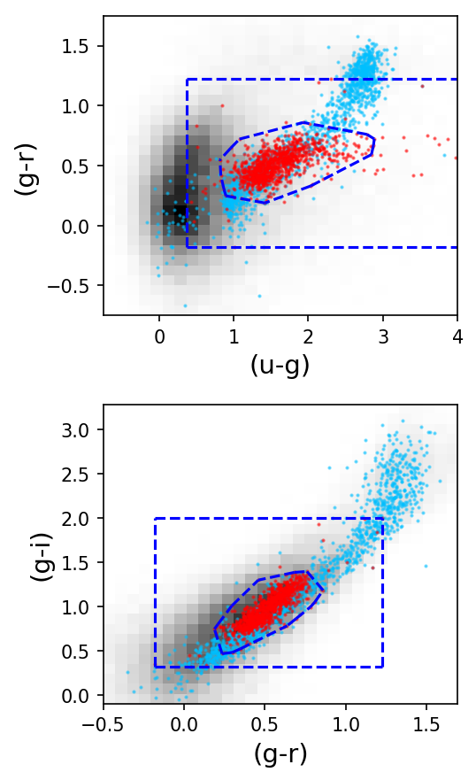
Figure 3: Colour-colour measurements of spectroscopic Fornax compact objects (red points), galactic stars (blue points) against the empirical distribution of all detected point sources over a subframe (greyscale histogram). Also shown are two colour selection boxes (blue dashed lines). In each panel, the large box corresponds to the minimum-bounding rectangle of compact object measurements in this colour-colour plane, and the smaller box is produced using the DBSCAN algorithm.

We note that we do not fit for the intrinsic colour distribution of GCs and interlopers as was done in Amorisco et al. (2018). The reason for this is that simple statistical representations (e.g. Gaussian) are inappropriate to describe our data in the multi-dimensional colour space. This can be gathered from the appearance of figure 3. It may be possible to include extra colour-terms in the mixture models described in $\S\ref{section:bayes}$, but we leave this for future work.

3.6 Bayesian Mixture Models

We adopt a simplified version of the Bayesian mixture modelling of Amorisco et al. (2018) to measure the properties of the GC systems of our target galaxies. We are similarly motivated to rescale the spatial coordinates of the GCCs into units of the 1$r_{e,r}$ (half-light radius of the galaxy) ellipse. Our model consists of two surface density components: A central Plummer profile to represent the GCs associated with the target galaxy,

$$\mathrm{\Sigma}(r,r_{h})=\frac{1}{\pi}\frac{1}{r_{h}^{2}(1+r^{2}/r^{2}_{h})^{2}}$$ (2)

where $r_{h}$ is the half number radius, in units of $r_{e,r}$, and a uniform distribution to represent the background, which mainly consists of stars, background galaxies and intra-cluster GCs. The presence of NGC1399 in the centre of Fornax means that its GC system may contribute to a non-uniform background in its vicinity. However, it can be shown that for our galaxies the gradient in the surface density of GCs belonging to NGC1399 is negligible, with a maximal gradient value of $\sim 10^{-4}$ objects arcmin^-3 in the vicinity of our sources. For this calculation, we have used the de Vaucouleurs’ fit to the GC system of NGC1399 from Bassino et al. (2006). The total model likelihood takes the form:

$$\mathcal{L}=\prod_{i=1}^{N_{\mathrm{GCC}}}\left[\frac{f\Sigma(r_{i},r_{h})}{\int_{0}^{r_{\mathrm{max}}}S(r^{\prime})\Sigma(r^{\prime},r_{h})r^{\prime}dr^{\prime}}+\frac{1-f}{\int_{0}^{r_{\mathrm{max}}}S(r^{\prime})r^{\prime}dr^{\prime}}\right]$$ (3)

where $i$ runs over all detected (and not masked) GCCs within the transformed radius $r_{\mathrm{max}}$ of the galaxy, which we fix as 15$r_{e,r}$; large enough to include all the galaxies’ GCs and a large number of background GCCs. We do not consider larger regions because of the increased potential of contamination from steep GCC gradients in the Fornax core. The spatial completeness function $S(r)$ encodes the fractional unmasked area as a function of radius. There are two free parameters: $f$, the mixing fraction (i.e. the fraction of all sources that are GCs belonging to the target galaxy) and the ratio $r_{h}$/$r_{e}$. We do not explicitly include morphological or colour terms in the model likelihood, but account for this in the GCC selection described in sections 3.2 and 3.5.

We impose a Gaussian prior on the ratio $r_{h}$/$r_{e}$ based on the results of Amorisco et al. (2018). The prior is centred at $\sim 1.5r_{e}$ with a standard deviation of 0.8 and truncated at zero. The choice of prior is very influential, particularly in the low $f$ regime in which most of our sources are anticipated to lie. However, since Amorisco et al. (2018) probe a similar sample of sources in a similar environment (the Coma cluster) to ours and that the $r_{h}$/$r_{e}\simeq 1.5r_{e}$ relationship appears elsewhere in the literature (van Dokkum et al., 2017; Lim et al., 2018) it is a reasonable estimate. We probe the effects of modifying the prior on $r_{h}$ in appendix D. The prior width is much greater than the RMS of the median values quoted by Amorisco et al. (2018), so that if there is any significant deviation it should be recognised in our analysis.

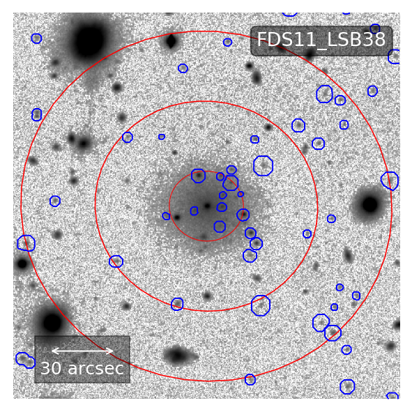
Figure 4: Result of full GCC identification and selection for one of our target galaxies. The selected sources are shown using their ProFound segments in blue. We also show the 1, 3 and 5 $r_{e,r}$ contours from the Imfit modelling. A clear over-density of sources can be seen close to the centre of the galaxy.

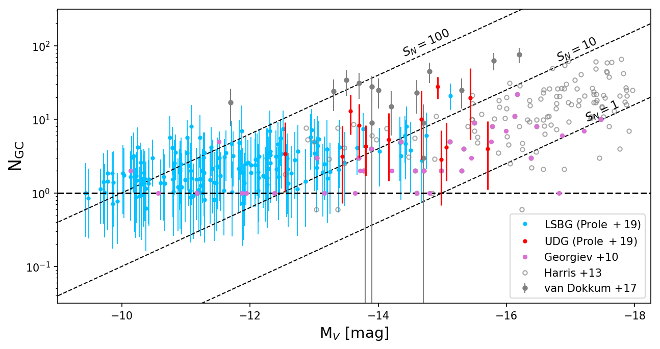
Figure 5: Corrected number counts of globular clusters as a function of absolute $V$-band magnitude. On the figure we show our new measurements in blue (LSBG sample) and red (UDG sample). The points represent median values from our MCMC posterior, and the errorbars span the range of the 1$\sigma$ uncertainties. The open grey circles belong to the Harris et al. (2013) catalogue. The grey points with error bars are the sample of selected Coma UDGs from van Dokkum et al. (2017). We also plot the sample of dwarf galaxies measured by Georgiev et al. (2010) in pink. The diagonal dashed black lines represent $S_{N}$ contours, whereas the horizontal one represents 1 GC.

4 Results

4.1 Inference on Globular Cluster numbers

We made data cut-outs in each band for each source that were 15$\times$15 $r_{e,r}$ in size. We chose this size because tests with mock datasets (with realistic numbers of interlopers derived from the data) revealed that the measured number of GCs was negatively biased for much smaller values, and this particularly affected systems with less than 10 intrinsic GCs. At 15$\times$15 $r_{e,r}$, we were able to recover unbiased measurements of $N_{\mathrm{GC}}$ even for systems with no GCs.

The GCCs were selected according to the criteria described in $\S$3.2 and by their colour, described in $\S$3.5. All non-selected sources were masked using their ProFound segments. We additionally automatically masked the areas around ProFound sources with $g$-band magnitudes brighter than 19 in an effort to remove interloping GCs belonging to other systems. This was accomplished by placing elliptical masks scaled to 2 times the ProFound R100 radius.

All sources in the GCC catalogues that had central coordinates overlapping with the masks were removed. The spatial completeness function could then be measured by measuring the masked fraction in concentric annuli centred on the galaxy, spaced by 0.01$r_{e,r}$ and linearly interpolating the result. We note that two sources were omitted from the analysis because they were almost completely masked.

We then ran the Monte-Carlo Markov chain (MCMC) code emcee to obtain the posterior distributions of $f$ and $r_{h}$ for each individual target galaxy. The final inference on the number of GCs associated with each galaxy, $N_{\mathrm{GC}}$, was calculated as

$$N_{\mathrm{GC}}^{j}=f^{j}\frac{\int_{0}^{r_{\mathrm{max}}}\Sigma(r,r_{h}^{j})rdr}{\int_{0}^{r_{\mathrm{max}}}S(r)\Sigma(r,r_{h}^{j})rdr}\frac{\int_{m_{\mathrm{1}}}^{m_{\mathrm{2}}}g(m)dm}{\int_{m_{\mathrm{1}}}^{m_{\mathrm{2}}}\epsilon(m)g(m)dm}N_{\mathrm{GCC}}$$ (4)

taking into account the masked fraction and magnitude incompleteness. Here, $j$ indicates the posterior index and $g(m)$ is the Gaussian $g$-band GCLF. The results of this are shown in figure 5, where we convert our galaxy photometry to $V$-band magnitudes using the prescriptions of Jester et al. (2005). As a means of comparison, we show in Appendix C that our inferences on $N_{\mathrm{GC}}$ are consistent with the measurements of Miller & Lotz (2007) for a small sample of overlapping galaxies using a chi-squared test.

We record the following information from the $N_{\mathrm{GC}}$ posterior: The 10th, 50th, and 90th percentiles, the 15.9 & 84.1 percentiles (i.e. the 1$\sigma$ limits centred on the median). The numbers we quote for $N_{\mathrm{GC}}$ are the median values and the uncertainties span the range of the 1$\sigma$ limits centred on the median; these are the error-bars shown in figure 5. Note that these estimates are corrected for the colour incompleteness from $\S$3.5. Trials with mock datasets showed that the median value is not significantly biased despite the marginal posterior in $f$ being naturally truncated at zero by our model. We find that 0 out of 12 UDGs have median values of $N_{\mathrm{GC}}$ below one, compared to 12 across the whole sample. However, 106 of the whole sample of target galaxies are consistent with having no GCs within $1\sigma$.

Overall, our results show a general increase of $N_{\mathrm{GC}}$ with $\mathrm{M}_{V}$ that is qualitatively consistent with normal dwarf galaxies. While some UDGs are comparable with those of van Dokkum et al. (2017), most of their objects are quite remarkable when compared to our measurements in terms of having much higher $N_{\mathrm{GC}}$ for a given luminosity. It remains to be seen whether these sources are comparatively rare among LSB galaxies and because Fornax contains less galaxies we see fewer UDGs with GC excess, or that perhaps the increase in environmental density in the Coma cluster plays a positive role in producing such galaxies; this is discussed further in $\S$5.

4.2 Colours

Despite already imposing a conservative colour selection criterion in $\S$3.5, we can use our results to assess the distribution of colour within the selection box. For each posterior sample, one can assign a probability of belonging to the Plummer profile (i.e. the galaxy) to each GCC given by

$$P_{\mathrm{GC}}(r)^{j}=\left[1+\frac{2(1-f^{j})\int_{0}^{r_{\mathrm{max}}}\Sigma(r^{\prime},r_{h}^{j})r^{\prime}dr^{\prime})}{f^{j}\Sigma(r,r_{h}^{j})r^{2}}\right]^{-1}$$ (5)

where $j$ loops over the posterior sample. The result of selecting high-probability GCCs is shown for a selection of galaxies in figure 6. We display the full colour distributions for all our GCCs weighted by their probabilities of cluster membership in figure 7. It is clear from these distributions that one-or-two component Gaussian fits are inappropriate, so we limit ourselves to a qualitative discussion based on the weighted histograms.

Comparing the weighted $(g-i)$ histogram with the un-weighted version, it is clear that a narrow peak emerges that is coincident with the blue component measured by D’Abrusco et al. (2016) at $<g-i>$=0.74. We conclude that the GC population of our sample is mainly blue. This is consistent with the results of Peng et al. (2006), who have shown that low luminosity galaxies tend to have predominantly blue GC systems. The blue nature of the GCs is suggestive of young and/or low-metallicity stellar populations.

In figure 7 we also show the $\pm 1\sigma$ span of the colours of the target galaxies. Clearly the blue peaks we observe in $(g-i)$ and $(g-r)$ are consistent with these colours. In $(g-r)$, the blue peak of the GCs appears shifted to the blue compared to the galaxy colours. However, since this effect is within the $1\sigma$, it is not a significant result.

4.3 Stellar mass vs Halo mass

Using our estimates of $N_{\mathrm{GC}}$ together with the empirical trend of Harris et al. (2017) (accounting for the intrinsic scatter in the relation), we are able to estimate the halo mass $M_{halo}$ of the sample of galaxies. For the estimate to be valid, one must assume that $N_{\mathrm{GC}}$ is indeed a reasonable indicator of $M_{halo}$ in the LSB regime. There is limited evidence to support this (Beasley et al., 2016; van Dokkum et al., 2017) based on comparisons between $M_{halo}$ measurements inferred from $N_{\mathrm{GC}}$ and those inferred from kinematic measurements. We also estimate the stellar mass using the empirical relation of Taylor et al. (2011) (their equation 8), who used the GAMA survey (Driver et al., 2011) to calibrate stellar mass as a function of $g$ and $i$ magnitudes with an intrinsic scatter of $\sim$0.1 dex.

We plot our estimates of $M_{halo}$ vs. $M_{*}$ in figure 8. We also display other measurements from the literature, including the sample of Coma UDGs from van Dokkum et al. (2017) and the median values measured by Amorisco et al. (2018) (it is worth noting that only three of their sources have $M_{halo}>10^{11}\mathrm{M_{\odot}}$ at 90% confidence), along with measurements of other dwarf galaxies, including dwarf ellipticals in clusters (Miller & Lotz, 2007) as well as late-type dwarfs from a variety of environments including the field (Georgiev et al., 2010). We also show the 2$\sigma$ credibility upper limit on the average mass of UDGs derived from weak lensing by Sifón et al. (2018), with which our results are consistent. Also we show the extrapolated theoretical predictions from abundance matching of Moster et al. (2010), Behroozi et al. (2013) and Brook et al. (2014), which were calibrated using observed stellar masses greater than approximately $10^{8}$, $10^{7}$ and $10^{7}\mathrm{M_{\odot}}$ respectively.

Forbes et al. (2018) show that the $N_{\mathrm{GC}}$ to $M_{halo}$ relation may lose accuracy for $M_{halo}\leq 10^{10}\mathrm{M_{\odot}}$, giving systematically higher values of $M_{halo}$ than measured for their sample. According to their study, a better estimator of $M_{halo}$ is the total mass associated with the GC system; however, they note that the assumption of a common mean GC mass is not valid at the low-mass end such that individual GC masses should be measured to get an unbiased estimate of $M_{halo}$, using the empirical relation of Spitler & Forbes (2009). While we have not measured the individual GC masses in this work, we note that our estimates of $M_{halo}$ should be considered as upper-limits in light of their result.

Every UDG in our sample is consistent with inhabiting a dwarf sized halo to within 1$\sigma$. There appears to be no significant tendency for UDGs to have enhanced GC populations and therefore enhanced halo mass for their stellar mass. Indeed, there is a qualitatively continuous trend from the LSBGs towards the UDGs.

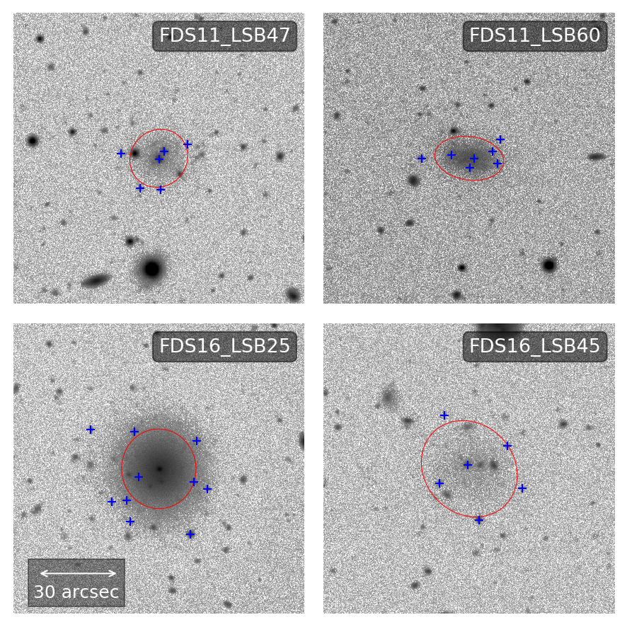
Figure 6: $r$-band cut-outs of four of our target galaxies, selected from galaxies with $N_{\mathrm{GC}}\geq$5. The red ellipses represent 1$r_{e,r}$ contours. The blue points identify GCCs with $P_{\mathrm{GC}}\geq 0.5$. Of the four galaxies shown, FDS16_LSB45 is the only one we measure to be large enough to be classified as a UDG. 30$\arcsec$ is $\sim$2.9kpc at Fornax distance.

The overall population is most consistent with an extrapolation of the Brook et al. (2014) relation (calibrated with local group dwarf galaxies), but we cannot rule out consistency with that of Moster et al. (2010) or Behroozi et al. (2013) because of the potential for our estimates of $M_{halo}$ to be overestimates. We emphasise however that all models require extrapolation, below stellar masses of 10${}^{8}\mathrm{M_{\odot}}$ for the Moster et al. (2010) relation, and 10${}^{7}\mathrm{M_{\odot}}$ for that of Behroozi et al. (2013) and Brook et al. (2014).

While no UDGs have estimates of $M_{halo}$ above what might be expected for enriched GC systems (according to the empirical relation of Amorisco et al., 2018), several of the LSBG sample do show evidence for excess. This might suggest a continuation of GC-enriched systems down to very low stellar mass.

Another point of interest is that our overall sample of LSB galaxies (including UDGs) appears offset from the mean trend of dwarf galaxies, having higher $M_{halo}$ for a given $M_{*}$. While our estimates of $M_{*}$ for the objects from the literature require assumptions about their colours, this may hint that LSB galaxies have systematically higher M/L ratios than normal dwarfs. However this might be a systematic effect; perhaps only LSB galaxies of high M/L ratio are able to survive in the Fornax core.

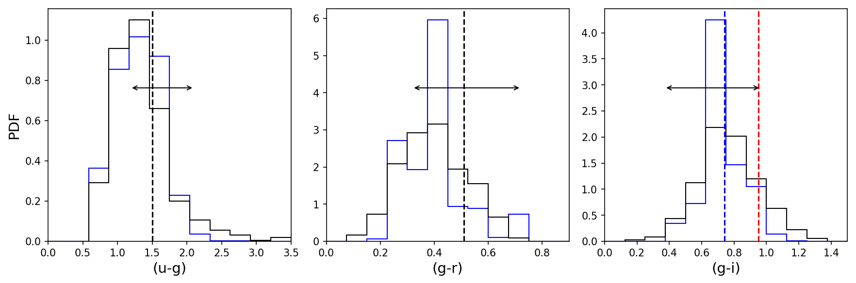
Figure 7: Normalised distribution of colours for the GCC sample (black histograms) vs. those of the same sample after being weighted by their probability of belonging to a target galaxy’s GC system according to equation 5 (blue histograms). We note that we select only sources with $m_{g}\leq 23$ to overcome the measurement error and ease comparison with D’Abrusco et al. (2016), who used a similar limit. For $(u-g)$ and $(g-r)$, the vertical black dashed lines correspond to the median colours of the sample of spectroscopic sources described in $\S$3.5. The dashed blue and red lines in the $(g-i)$ panel correspond to the means of the blue and red components measured by D’Abrusco et al. (2016). The results a consistent with a predominantly blue GC population. The horizontal arrows indicate the $\pm 1\sigma$ range of the galaxy colours.

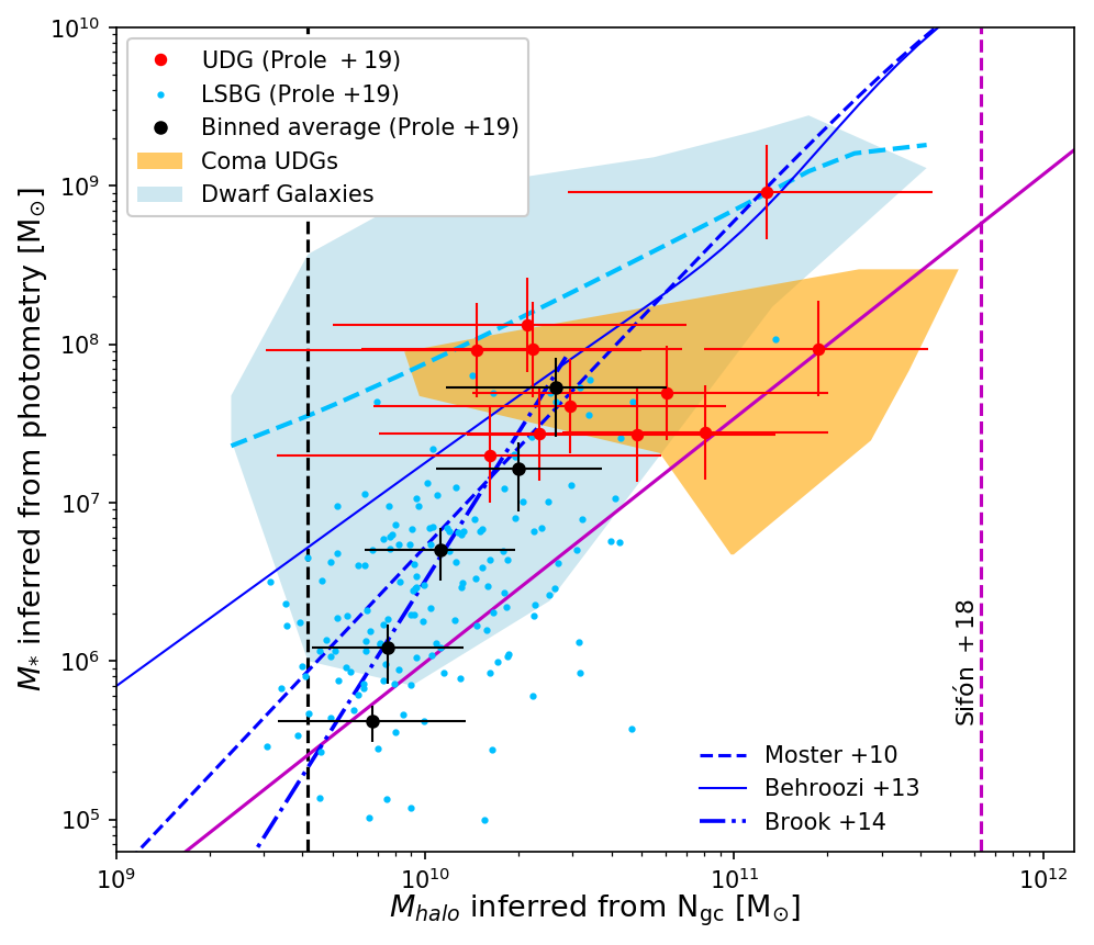
Figure 8: Halo mass (derived using $N_{\mathrm{GC}}$) vs. stellar mass. In the figure we show our new measurements, the light blue points correspond to LSBGs and the red to UDGs. The stellar masses for our points were derived from $g$ and $i$ band photometry using the scaling relation of Taylor et al. (2011). The black error-bars show illustrative binned averages of all our new measurements (calculated in logarithmic bins). The orange region bounds UDG measurements from the literature (van Dokkum et al., 2017; Amorisco et al., 2018; Lim et al., 2018), We also plot measurements of other “normal” dwarf galaxies (Miller & Lotz, 2007; Georgiev et al., 2010, blue region). The dashed light blue line represents the mean of these sources. The darker blue lines show extrapolated theoretical predictions of Moster et al. (2010), Behroozi et al. (2013) & Brook et al. (2014). The diagonal purple line corresponds to “enhanced” GC systems Amorisco et al. (2018), using the Harris et al. (2017) conversion between $N_{\mathrm{GC}}$ and $M_{halo}$. The dashed purple line indicates the 2$\sigma$ credibility upper-limit on the average mass of UDGs derived from weak lensing Sifón et al. (2018). Finally, the vertical black dashed line corresponds to $N_{\mathrm{GC}}=1$.

4.4 GC system sizes

Despite imposing a prior on $r_{h}$ (the GC half number radius) with a mean of 1.5$r_{e}$, we find that our GC systems are typically slightly larger. The median value of $r_{h}$ recovered from the full sample of galaxies is 1.73, with a standard deviation of $\sim 0.27$ and range between 0.4 and 2.8 (in units of $r_{e,r}$). We note that the median value of $r_{h}$ for the UDGs is consistent with that of the full sample.

If we use the relation between $r_{h}$ and $M_{halo}$ presented in Hudson & Robison (2018), the resulting $M_{halo}$ estimate is much larger than previously estimated using $N_{\mathrm{GC}}$. For example, for a UDG with $r_{h}$=1.5 kpc should have $M_{halo}$ of around $10^{11.6}\mathrm{M_{\odot}}$, much higher than many of the estimates presented in figure 8 and generally inconsistent with UDGs with halo mass measurements in the literature (e.g. van Dokkum et al., 2017). While we note that Hudson & Robison (2018) make clear that the relation is calibrated only for $M_{halo}\geq 10^{12}\mathrm{M_{\odot}}$, we advocate a relation more in-line with that of Forbes (2017) in this regime.

4.5 LSBGs vs UDGs

Now that we have estimates of $N_{\mathrm{GC}}$ for each of our target galaxies, we are in a position to directly compare the LSBG population with the UDGs. The two questions we want to answer are: Does the UDG population show any statistical excess of GCs when compared with the LSBGs in the same luminosity range?; and, is the observed distribution of $N_{\mathrm{GC}}$ for the UDGs discontinuous from that of the LSBGs?

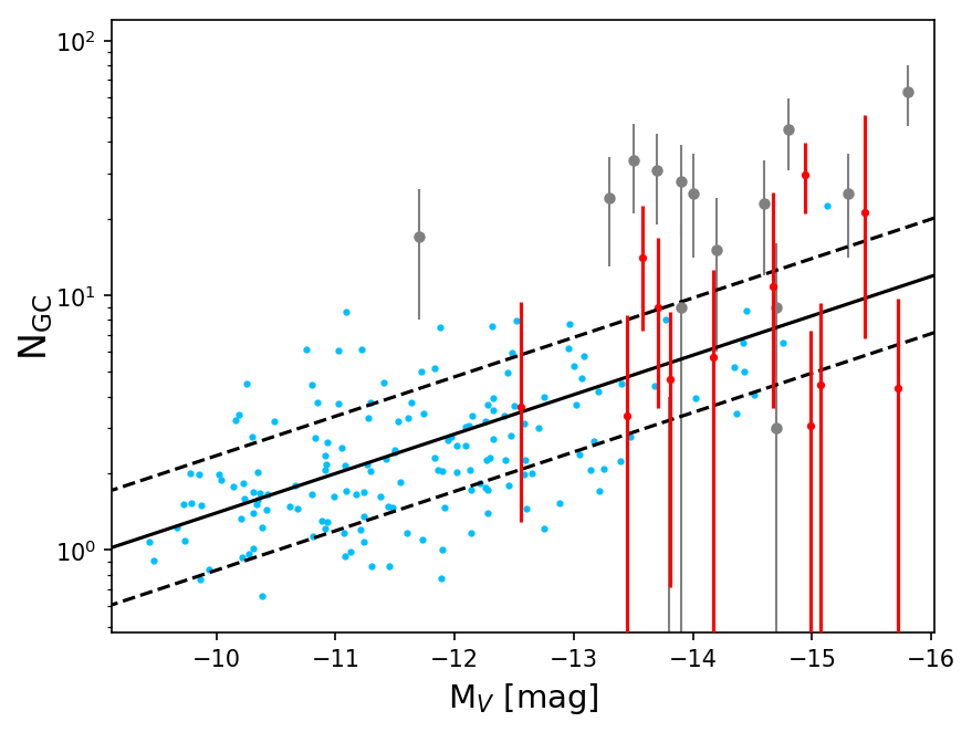
Figure 9: Power-law fit to $N_{\mathrm{GC}}$ vs. M_V for our LSBG sample (solid black line) along with an estimate of the 1$\sigma$ scatter (black dashed lines). Blue points: Our LSBG sample. Red errorbars: Our UDG sample. Grey errorbars: The sample of GC-enriched UDGs from van Dokkum et al. (2017).

We note that from the appearance of figure 5, it seems that $N_{\mathrm{GC}}$ vs. $\mathrm{M}_{V}$ can be modelled approximately as a power law. We omit all UDGs from the sample and fit such a relation to our LSBG sample (see also figure 9):

$$\bar{N}_{\mathrm{GC}}=(0.04\pm 0.02)\times 10^{(-0.15\pm 0.02)\times\mathrm{M}_{V}}$$ (6)

We note that the scatter in the relation is approximately 0.2 dex across the full magnitude range. Using the fit, we can ask whether our sample of UDGs (ignoring other UDGs from the literature) are consistent with this description. We perform a chi-squared test with the null-hypothesis that the UDGs are drawn from equation 6. This results in a $p$-value of 0.30, which means we cannot reject the null hypothesis with an acceptable level of confidence. We therefore conclude that our UDG sample is quantitatively consistent with a continuation of the LSBG sample in this parameter space. We also note that since there is no UDG that has a $N_{\mathrm{GC}}$ measurement convincingly more than 3$\sigma$ above the power-law predicted value, there is no compelling evidence that our UDGs have excessive GC populations.

As as means of comparison, we also do the same test for the population of GC-enriched UDGs from van Dokkum et al. (2017). While the two tests are not directly comparable since the sample of van Dokkum et al. (2017) is was at-least partially biased to select extreme objects (as in the cases of galaxies DF44 and DFX1), we find that their sample is not consistent with equation 6, with a $p$-value much less than 1%.

Aside from DF44 and DFX1, the galaxies measured by van Dokkum et al. (2017) also include a list of 12 UDGs selected from the Yagi et al. (2016) catalogue of LSB galaxies that are also present in the Coma Cluster Treasury Program footprint. Importantly, this should represent a small but unbiased sample of Coma UDGs. After selecting only these sources and repeating the test, we find that the Coma sample is still inconsistent with equation 6. This may indicate that UDGs in Coma have more GCs than galaxies in Fornax in the same luminosity range. We find that the choice in prior for the GC half-number radius does not impact this result; for a detailed discussion see appendix D.

4.6 Effect of the GCLF

As stated in $\S$3.4, we have adopted a Gaussian GCLF with a mean of 24$m_{g}$ and standard deviation of 0.7$m_{g}$. However, dwarf galaxies can have varied GCLFs and it is important to show that our results are robust against this. Villegas et al. (2010) have measured the $g$-band GCLFs for 43 early-type galaxies in the Fornax cluster, down to galaxies with absolute $B$-band magnitudes of around -16. We use this catalogue as a means to test what would happen to our measurements if the GCLF was wider and has turnover magnitude fainter than our adopted value, i.e. to get an upper-limit on the inferences on $N_{\mathrm{GC}}$.

From the Villegas et al. (2010) catalogue, we measure a mean GCLF with mean 24$\pm$0.1$m_{g}$ and a standard deviation of 0.84$\pm$0.21$m_{g}$ after clipping outliers at $2\sigma$. We note that we selected from their catalogue only galaxies with absolute $B$ magnitudes fainter than -18 to target dwarf galaxies for this calculation. This suggests that the GCLF might be wider than what we have assumed previously. Integrating the RE over the $1\sigma$ deeper and wider GCLF and comparing to our previous estimates of the observed GC fraction, we find that the maximum correction in our $N_{\mathrm{GC}}$ is an increase of $\sim$20%. We find that this is not sufficient to impact or change the overall results of our work (a 20% increase in $N_{\mathrm{GC}}$ is sufficient to increase a $M_{halo}$ estimate by $\sim$0.1dex).

4.7 Effect of Nuclear Star Clusters

We do not treat potential NSCs any differently from GCs in our analysis; GCCs are defined by their magnitude and colour. While we have imposed a bright-end magnitude cut on our sample of GCCs, there is still potential for faint NSCs to contaminate our sample and therefore increase the number of GCCs for a target galaxy by one. For the galaxies with low estimates of $N_{\mathrm{GC}}$, this can amount to a significant source of error. However, most of our target galaxies have $M_{*}\leq 10^{8}\mathrm{M_{\odot}}$ and are thus expected to have a low nucleation fraction (between 0.7 at $10^{8}\mathrm{M_{\odot}}$ to 0.0 at $10^{5}\mathrm{M_{\odot}}$, as shown in figure 8 of Sánchez-Janssen et al., 2018).

Removing GCCs close to the centres of galaxies introduces a subjective bias. However, we note that all the galaxies in our sample have already been visually classified as either nucleated or non-nucleated by Venhola et al. (2017). This number amounts to 10% of the catalogue. After applying our bright-end magnitude cut, this leaves us with 13 galaxies that are potentially contaminated by a NSC. To quantify the effect this may have on our estimates of $M_{halo}$, we simply drop these sources from the sample and repeat the analysis. We find that the results do not change; the new binned-average estimates of $M_{halo}$ are consistent within much less than $1\sigma$ with those displayed in figure 8.

5 Discussion and Conclusions

In this paper we have estimated the halo masses of a sample of 175 LSB galaxies in the Venhola et al. (2017) catalogue using the sizes of their GC populations, including a sub-sample of 12 UDGs. This constitutes the largest sample of low mass galaxies so-far analysed for this kind of study. Candidate globular clusters were identified in the $g$-band using measurements from the ProFound photometry package. We also applied a colour selection based on photometric measurements of a set of spectroscopically confirmed Fornax cluster GCs, using PSF-corrected aperture magnitudes measured in the $u,g,r,i$ bands. Following this, we used a Bayesian Mixture model approach (influenced by the work of Amorisco et al., 2018) to infer the total number of GCs associated with each target galaxy, assuming a GCLF appropriate for our sample.

Our estimates of $N_{\mathrm{GC}}$ for the overall population are qualitatively consistent with more compact dwarf galaxies when plotted against $\mathrm{M}_{V}$. We find that the sample of UDGs are statistically consistent with a power-law fit to the $N_{\mathrm{GC}}$ measurements for LSBGs, indicating that there is no discontinuity between the two populations; our sample of UDGs does not have a statistically significant excess of GCs compared to smaller LSB galaxies in the same luminosity range.

We converted the inferences on $N_{\mathrm{GC}}$ to $M_{halo}$ using the empirical relation of Harris et al. (2017). We additionally derived stellar masses for the galaxies from the empirical relation of Taylor et al. (2011), using Imfit galaxy models. Overall, the $M_{*}$ estimates are consistent with dwarf galaxies and the $M_{halo}$ estimates are consistent with dwarf sized halos. The LSBG galaxy population appears consistent with the extrapolated Brook et al. (2014) abundance-matching relation between $M_{*}$ and $M_{halo}$ and as an extension of measurements from typical dwarf galaxies, but perhaps with slightly larger $M_{halo}$ for the average dwarf at a given $M_{*}$. We suggest that this might be a systematic effect due to the environment; it is possible that only LSB galaxies with high M/L ratios are able to survive in the Fornax core. However, as Forbes et al. (2018) have shown, the $M_{halo}$ estimates may be too large because of a breakdown in accuracy of the $N_{\mathrm{GC}}$-$M_{halo}$ relation in the low mass regime, and it is not yet clear how this affects our estimates.

None of our UDGs have median values of $N_{\mathrm{GC}}$ above the empirical boundary marking GC-rich systems measured by Amorisco et al. (2018). However, 5 are consistent within their 1$\sigma$ uncertainties. Several LSBGs also have potential for GC-richness, and 13 are at least 1$\sigma$ above the required threshold. Such objects could make interesting sources for a follow-up study, given that they could represent a continuation of GC-rich objects down to very low stellar mass. If genuine, they could mean that enhanced GC systems are not unique to UDGs and the mechanisms by which UDGs are produced are separate from those by which LSB galaxies gain enriched GC systems, something also observed by Amorisco et al. (2018).

Using a weighted histogram approach, we have shown that the GC population of our target galaxies is predominantly blue compared to the overall GC population in Fornax. Our result is consistent with the blue peak in $(g-i)$ recorded by D’Abrusco et al. (2016), with a relative depletion of red GCs. Further still, the blue peak of our GC coincides with the $\pm 1\sigma$ range of the galaxy colours. There is tentative evidence in $(g-r)$ that the galaxies may be slightly redder than the GCs, but since this is not a significant effect we do not comment on this further.

The Coma cluster UDGs measured by van Dokkum et al. (2017) seem to have significantly more GCs than what we see in the Fornax cluster. It is notable that our sample is confined to the core of the Fornax cluster. While Lim et al. (2018) show that there is no particular trend of specific frequency $S_{N}$ with cluster-centric radius for bright UDGs in Coma, they also show that $S_{N}$ decreases with cluster-centric radius for fainter galaxies; if anything this could mean that we probe a population with systematically higher $N_{\mathrm{GC}}$ at a given $M_{*}$ than in the cluster outskirts. Two possibilities are that GC-enriched UDGs are comparatively rare objects and we simply do not observe them because Fornax is much less massive than Coma, or the denser environment of the Coma cluster plays a positive role in UDG GC formation or acquisition. We suggest that future studies could provide complete measurements of $N_{\mathrm{GC}}$ for UDGs in other clusters (e.g. Virgo) to address this question.

Our measurements are sufficient to rule out the failed $L_{*}$ formation theory for UDGs because the halo mass estimates indicate that they reside in dwarf sized halos. We find a continuation in properties between UDGs and smaller LSBGs such that it does not seem that UDGs have a unique or special formation mechanism. Since few of our UDGs are convincingly GC-rich compared to those in Coma, we speculate that this property may be related to environmental density. Perhaps the Coma objects are more efficiently stripped of gas in the Coma core, thus forming fewer stars relative to their halo mass, resulting in systems that appear GC-rich for their stellar mass. A consequence of this effect is that the fraction of GC-rich UDGs should decline with cluster-centric radius, and this may be a valuable way to estimate the relative strengths of secular vs. environmentally-driven formation mechanisms.

Appendix A Galaxy Modelling

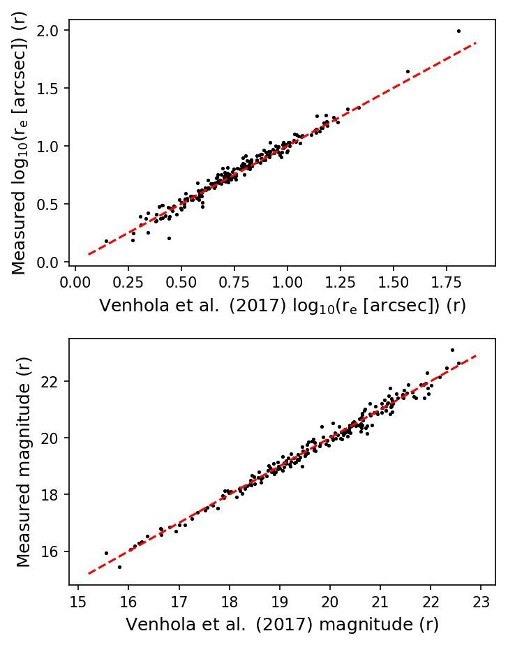
Figure 10: Our galaxy measurements (Imfit ) vs. those of V17 (GALFIT). Red dashed line: The one-to-one relation. The RMS of the residuals are 0.18 mag and 0.04 dex in $r_{e}$.

We used Imfit  to fit single Sérsic profiles to each target galaxy. Fortunately, Venhola et al. (2017) (hereafter V17) already provide such fits in the $r$-band. While here we choose to remeasure the profiles for consistency with the other bands, we do make use of these data as initial guesses in the fitting. Our approach was to iteratively fit the galaxy in the $r$-band, each time improving the mask of pixels to ignore in the fit. The general procedure for a galaxy is as follows:

1. Obtain an $8\times 8r^{r}_{e,V17}$ $r$-band cut-out.

2. Subtract the V17 model from the result (include nuclear PSF if indicated by V17).

3. Use DeepScan (Prole et al., 2018) to get sky and RMS estimates from the result.

4. Create a smoothed image by applying a Gaussian filter with RMS=2 pixels.

5. Mask all pixels with $\geq 6\sigma$ significance on the smoothed image.

6. Use Imfit  to fit a Sérsic model to the original data with the sky subtracted, ignoring pixels in the mask.

7. Repeat steps 2 to 6 three times, each time updating the model image and mask.

8. Repeat steps 1, 3 & 6 for the other bands, using the same $r$-band mask in each.

For the DeepScan sky estimates we used a mesh size equal to the image size and performed three masking iterations. If the galaxy was indicated as nucleated by V17, we also fit a Moffat profile simultaneously with the Sérsic model. We found that in a minority of cases the residuals from the V17 fits were quite large, such that we had to modify the masks manually.

In the case of FDS11_LSB2, the largest galaxy in our sample (with $r^{r}_{e,V17}=76\arcsec$), we re-binned the data by a factor of 5 to make the fit easier (the original fitting region was $\sim 3000\times 3000$ pixels). Over this region the sky background level varies significantly, so we modified the DeepScan sky modelling to use mesh sizes of $\sim 200\arcsec$ and median filtered in $3\times 3$ meshes. We note that an image of FDS11_LSB2 is displayed in figure 20 of V17.

Overall our results are consistent with V17 (figure 10), with a few exceptions. These include FDS11_LSB2, which we measure to be 1.5 times larger than originally reported. This result was robust against changes in the size of the background mesh. We also note that we measure a slightly lower Sérsic index $n$ for this object, and $n$ is generally anti-correlated with $r_{e}$. This discrepancy likely arises from the difficulty involved in measuring such a large, diffuse galaxy in a reasonably crowded field with a varying sky; we use DeepScan whereas V17 fit a 2D sky plane in their GALFIT (Peng et al., 2002) modelling. We also note that V17 did not leave the central coordinate of their model profiles as a free parameter.

Finally, we note that we were not able to obtain stable Imfit models for several sources because they were too faint: FDS12_LSB42, FDS12_LSB47, FDS11_LSB16 & FDS12_LSB34. We therefore adopted the fits of V17 for these sources. Since V17 did not measure $(g-i)$ colours, we have omitted them from stellar mass calculations and from figure 8.

Appendix B Photometric Calibration

Starting from the VSTtube-reduced data, we used ProFound to detect and select point sources. We additionally measured fixed-aperture magnitudes for each source with an estimate of that magnitude. These aperture magnitudes had to be corrected for both the limited size of the aperture with respect to the PSF in each band, but also the absolute calibration to AB magnitudes.

While there is no ideal set of standard stars in our footprint with which to calibrate the photometry, Cantiello et al. (in prep) have used a set of existing, overlapping calibrated catalogues (ACSFCS (Jordán et al., 2007); APASS (Henden et al., 2012); SkyMapper (Wolf et al., 2018)) to calibrate their photometry in the same data. We have calibrated our own aperture magnitudes by matching our catalogue with theirs, selecting point sources as in $\S$3.2 and applying a multiplicative correction to our measurements to nullify the mean offset between the measurement pairs. The RMS between our corrected aperture magnitudes with theirs is $\sim$0.05 mag in $g,r,i$ and $\sim 0.2$ mag in the shallower $u$-band, for all matching point sources with corrected $g$ magnitudes brighter than 23 mag.

During the calibration it was noticed that the reference catalogue of Cantiello et al. (in prep) contained minor systematic offsets in the stellar locus between individual FDS frames, suggesting a systematic error in the absolute calibration. We have dealt with this by shifting each locus to a common position in colour-colour space. The net result of this is a maximum systematic uncertainty of $\sim\pm 0.05$ mag in each colour plane. Finally, we note that since there is currently no available reference catalogue for FDS frame 12 we calibrated the photometry for that frame in accordance with FDS frame 11. This calibration is accurate enough to have negligible effects on our results.

Appendix C Comparison with Miller and Lotz (2007)

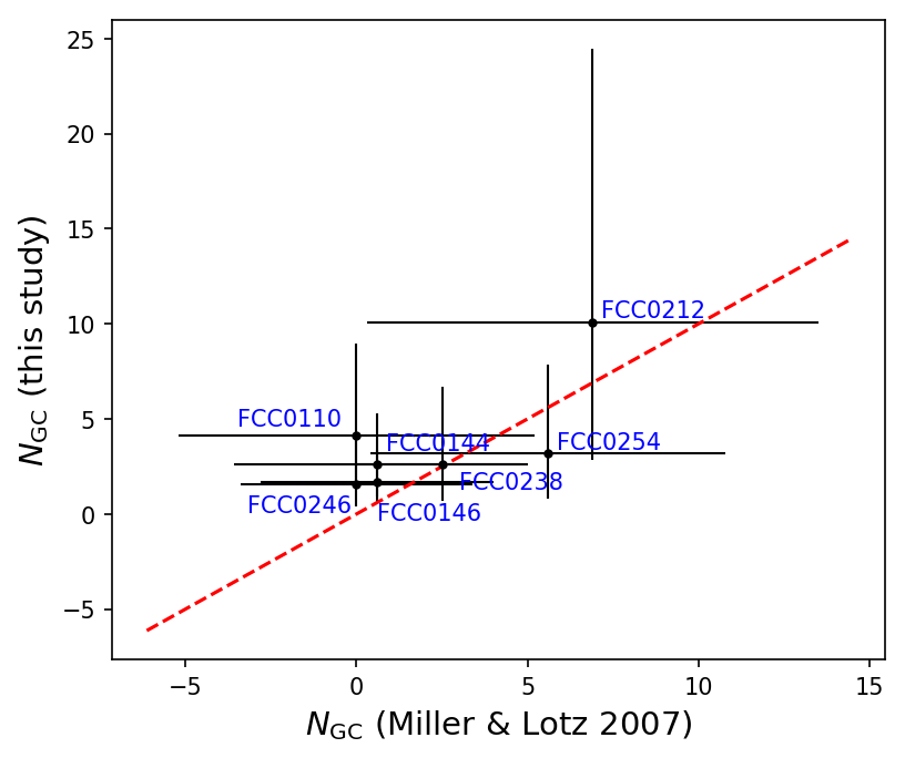
Figure 11: Comparison of GC number counts. The black points are median values from the MCMC posterior. The error-bars span the range of $1\sigma$. The red dashed line is the one-to-one relation. A chi-square test (accounting for the errors) shows that the null hypothesis that the measurements are consistent with the one-to-one relation cannot be rejected with confidence greater than around 4%.

As several of the sources in the Venhola et al. (2017) catalogue were also identified in the Fornax cluster catalogue (Ferguson, 1989), we were encouraged to search for matches in the catalogue of dwarf ellipticals studied by Miller & Lotz (2007), who used the HST WFPC2 Dwarf Elliptical Galaxy Snapshot Survey to measure the GC populations for a sample of 69 galaxies. They measured $N_{\mathrm{GC}}$ using apertures of 5 times the exponential scale size of the galaxies, which roughly equates to 3$r_{e}$ for a Sérsic index $n$=1.

We find seven matches: FDS16_LSB33 (FCC0146), FDS12_LSB10 (FCC0238), FDS12_LSB4 (FCC0246), FDS11_LSB62 (FCC0254), FDS16_LSB58 (FCC0110), FDS16_LSB32 (FCC0144) and FDS12_LSB30 (FCC0212). Overall our results are reasonably consistent (albeit with large error-bars), as is shown in figure 11. Note that in the figure one of the sources is not visible because it overlaps with another.

Appendix D Choice of prior

While the choice for the prior on the GC half-number radius $r_{h}$ is justified from previous literature measurements (van Dokkum et al., 2017; Amorisco et al., 2018; Lim et al., 2018), it is important to show how different choices may affect the results. This is particularly relevant because the spatial distributions of GCs for UDGs is not well known. By running the MCMC using different priors, we show in figure 12 that, despite the choice of prior in $r_{h}$ strongly influencing the $r_{h}$ posterior, the estimates of $N_{\mathrm{GC}}$ are robust.

A small increase in the mean of the prior on the GC half-number radius, $\bar{r}_{h,prior}$, is not sufficient to significantly impact our results. However, more dramatic modifications may produce a more pronounced change. In general, lowering $\bar{r}_{h,prior}$ increases the number of GC-poor systems, while increasing it results in more GC rich systems. However, the median value for the overall population is not significantly altered by using different priors. We finally note that repeating the analysis from $\S$4.5 with $\bar{r}_{h,prior}$=3$r_{e}$ leads us to the same conclusions; the overall result is robust against changes in the prior.

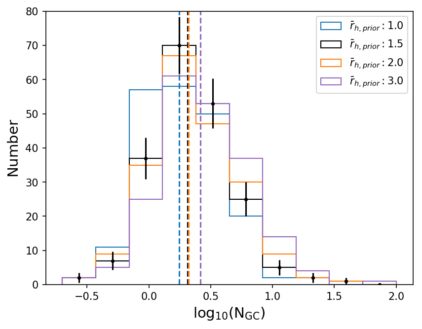
Figure 12: The distribution of $N_{\mathrm{GC}}$ estimates for our sample of galaxies as a function on the mean of the prior on the GC half-number radius, $\bar{r}_{h,prior}$, in units of galaxy half-light radius. Also shown are the median values (dashed lines). Our value of $\bar{r}_{h,prior}$=1.5$r_{e}$ is adopted from the literature and Poisson error-bars are shown for this value.

Appendix E Measurements table

Table 2: Results of our analysis. Values enclosed in braces are 10th, 50th and 90th percentiles from the MCMC posterior. Fiducial errors on $M_{V}$ and $M_{*}/\mathrm{M_{\odot}}$ are $\sim 0.2$ mag and 0.3 dex respectively. For $r_{e,r}$ the uncertainty is approximately 10% of the value after measuring the scatter between our measurements and those of Venhola et al. (2017). We remind the readers that the estimates of $M_{halo}$ should be considered as upper-limits.

Target	MV [mag]	$r_{e,r}$ [kpc]	$\log_{10}\left(M_{*}\ [\mathrm{M_{\odot}}]\right)$	$r_{h}[r_{e,r}]$	$N_{\mathrm{GC}}$	$\log_{10}\left(M_{halo}\ [\mathrm{M_{\odot}}]\right)$
FDS10_LSB2	-11.0	0.46	6.3	$\left\{1.06,2.04,2.94\right\}$	$\left\{0.7,3.7,9.4\right\}$	$\left\{9.5,10.3,10.7\right\}$
FDS10_LSB3	-9.8	0.64	6.3	$\left\{0.57,1.39,2.40\right\}$	$\left\{0.4,2.0,4.9\right\}$	$\left\{9.2,10.0,10.4\right\}$
FDS10_LSB4	-11.7	0.39	6.5	$\left\{0.69,1.65,2.66\right\}$	$\left\{0.2,1.1,3.5\right\}$	$\left\{8.7,9.7,10.2\right\}$
FDS10_LSB5	-11.1	0.94	5.6	$\left\{1.35,2.28,3.27\right\}$	$\left\{2.2,8.6,19.6\right\}$	$\left\{10.0,10.7,11.1\right\}$
FDS10_LSB6	-10.4	0.30	5.8	$\left\{0.77,1.75,2.79\right\}$	$\left\{0.3,1.4,3.4\right\}$	$\left\{9.0,9.8,10.2\right\}$
FDS10_LSB8	-11.3	0.69	6.3	$\left\{0.78,1.73,2.73\right\}$	$\left\{0.3,2.0,6.2\right\}$	$\left\{9.1,10.0,10.5\right\}$
FDS10_LSB9	-9.9	0.35	5.8	$\left\{0.66,1.37,2.36\right\}$	$\left\{0.5,2.0,4.6\right\}$	$\left\{9.3,10.0,10.4\right\}$
FDS10_LSB10	-11.3	0.62	6.2	$\left\{0.64,1.60,2.65\right\}$	$\left\{0.1,0.9,2.9\right\}$	$\left\{8.6,9.6,10.1\right\}$
FDS10_LSB13	-10.2	0.40	5.9	$\left\{0.72,1.51,2.52\right\}$	$\left\{0.4,1.8,4.5\right\}$	$\left\{9.2,9.9,10.4\right\}$
FDS10_LSB14	-11.1	0.50	5.6	$\left\{0.71,1.69,2.69\right\}$	$\left\{0.2,1.2,3.6\right\}$	$\left\{8.9,9.7,10.2\right\}$
FDS10_LSB15	-11.3	0.53	6.5	$\left\{0.43,1.18,2.27\right\}$	$\left\{0.5,2.2,5.0\right\}$	$\left\{9.3,10.0,10.4\right\}$
FDS10_LSB16	-10.6	0.34	6.1	$\left\{0.79,1.62,2.54\right\}$	$\left\{0.3,1.5,3.6\right\}$	$\left\{9.0,9.8,10.2\right\}$
FDS10_LSB23	-12.6	0.78	6.7	$\left\{0.92,1.91,2.94\right\}$	$\left\{0.4,2.3,7.2\right\}$	$\left\{9.1,10.0,10.6\right\}$
FDS10_LSB25	-14.2	2.06	7.6	$\left\{0.85,1.80,2.81\right\}$	$\left\{1.0,5.7,15.9\right\}$	$\left\{9.6,10.5,11.0\right\}$
FDS10_LSB29	-13.4	0.85	7.1	$\left\{0.74,1.64,2.61\right\}$	$\left\{0.4,2.2,6.5\right\}$	$\left\{9.1,10.0,10.5\right\}$
FDS10_LSB35	-12.3	0.35	6.6	$\left\{0.74,1.70,2.65\right\}$	$\left\{0.2,1.4,4.0\right\}$	$\left\{8.9,9.8,10.3\right\}$
FDS10_LSB38	-12.0	0.78	6.5	$\left\{0.19,1.05,2.15\right\}$	$\left\{0.8,2.8,6.7\right\}$	$\left\{9.5,10.1,10.5\right\}$
FDS10_LSB40	-11.0	0.90	6.1	$\left\{1.19,1.92,2.73\right\}$	$\left\{2.1,6.1,11.9\right\}$	$\left\{10.0,10.5,10.8\right\}$
FDS10_LSB41	-12.3	0.63	6.8	$\left\{0.73,1.64,2.64\right\}$	$\left\{0.4,2.3,7.8\right\}$	$\left\{9.1,10.0,10.6\right\}$
FDS10_LSB43	-11.1	0.51	6.2	$\left\{0.71,1.72,2.71\right\}$	$\left\{0.1,0.9,3.6\right\}$	$\left\{8.7,9.6,10.2\right\}$
FDS10_LSB44	-11.1	0.31	6.3	$\left\{0.30,0.95,2.15\right\}$	$\left\{0.5,1.7,3.7\right\}$	$\left\{9.3,9.9,10.3\right\}$
FDS10_LSB45	-12.1	0.53	6.7	$\left\{0.85,1.84,2.80\right\}$	$\left\{0.3,1.7,5.6\right\}$	$\left\{9.0,9.9,10.5\right\}$
FDS10_LSB46	-10.7	0.29	5.9	$\left\{0.66,1.58,2.63\right\}$	$\left\{0.2,1.4,4.5\right\}$	$\left\{8.8,9.8,10.3\right\}$
FDS10_LSB49	-12.3	0.55	6.8	$\left\{0.81,1.74,2.79\right\}$	$\left\{0.3,1.7,5.3\right\}$	$\left\{9.0,9.9,10.4\right\}$
FDS10_LSB51	-12.1	0.80	6.8	$\left\{0.91,1.81,2.79\right\}$	$\left\{0.4,2.6,7.2\right\}$	$\left\{9.2,10.1,10.6\right\}$
FDS10_LSB52	-13.8	1.54	7.4	$\left\{0.41,1.12,2.36\right\}$	$\left\{1.3,4.7,10.5\right\}$	$\left\{9.8,10.4,10.8\right\}$
FDS10_LSB53	-11.5	0.57	6.5	$\left\{0.52,1.25,2.31\right\}$	$\left\{0.4,1.8,4.6\right\}$	$\left\{9.2,9.9,10.4\right\}$
FDS10_LSB54	-9.7	0.33	6.7	$\left\{0.96,1.82,2.66\right\}$	$\left\{0.3,1.2,2.6\right\}$	$\left\{9.0,9.7,10.1\right\}$
FDS10_LSB55	-12.4	0.55	7.0	$\left\{0.88,1.77,2.75\right\}$	$\left\{1.2,5.0,11.4\right\}$	$\left\{9.7,10.4,10.8\right\}$
FDS10_LSB56	-9.7	0.47	5.4	$\left\{0.68,1.62,2.65\right\}$	$\left\{0.2,1.1,3.2\right\}$	$\left\{8.7,9.7,10.2\right\}$
FDS11_LSB4	-11.2	0.46	5.9	$\left\{0.70,1.77,2.72\right\}$	$\left\{0.3,1.7,5.5\right\}$	$\left\{9.0,9.9,10.4\right\}$
FDS11_LSB6	-10.3	0.63	6.6	$\left\{0.53,1.31,2.33\right\}$	$\left\{0.5,2.0,5.0\right\}$	$\left\{9.3,10.0,10.4\right\}$
FDS11_LSB7	-10.8	0.76	7.7	$\left\{1.26,2.05,2.92\right\}$	$\left\{1.6,6.1,13.9\right\}$	$\left\{9.8,10.5,10.9\right\}$
FDS11_LSB8	-10.3	0.48	6.2	$\left\{0.76,1.71,2.70\right\}$	$\left\{0.2,1.5,4.5\right\}$	$\left\{8.9,9.8,10.3\right\}$
FDS11_LSB10	-11.9	0.81	6.5	$\left\{0.53,1.38,2.44\right\}$	$\left\{0.5,2.1,5.0\right\}$	$\left\{9.2,10.0,10.4\right\}$
FDS11_LSB11	-10.9	0.56	6.3	$\left\{0.96,1.86,2.76\right\}$	$\left\{0.4,2.6,7.2\right\}$	$\left\{9.2,10.1,10.6\right\}$
FDS11_LSB13	-11.1	0.48	6.3	$\left\{0.96,1.97,2.93\right\}$	$\left\{0.3,2.2,6.3\right\}$	$\left\{9.0,10.0,10.5\right\}$
FDS11_LSB14	-11.8	1.07	7.3	$\left\{0.84,1.82,2.78\right\}$	$\left\{0.3,2.3,7.1\right\}$	$\left\{9.1,10.0,10.6\right\}$
FDS11_LSB15	-12.3	0.71	7.3	$\left\{0.79,1.69,2.65\right\}$	$\left\{0.7,3.9,11.4\right\}$	$\left\{9.5,10.3,10.8\right\}$
FDS11_LSB16	-12.5	1.50	–	$\left\{0.88,1.79,2.75\right\}$	$\left\{0.7,3.6,12.0\right\}$	$\left\{9.4,10.2,10.8\right\}$
FDS11_LSB18	-10.9	0.61	5.6	$\left\{0.08,0.44,1.94\right\}$	$\left\{0.6,2.2,5.1\right\}$	$\left\{9.4,10.0,10.4\right\}$
FDS11_LSB30	-13.7	1.75	7.4	$\left\{1.12,1.92,2.79\right\}$	$\left\{2.2,8.9,20.3\right\}$	$\left\{10.0,10.7,11.1\right\}$
FDS11_LSB35	-11.3	0.69	6.0	$\left\{0.73,1.45,2.43\right\}$	$\left\{0.9,3.8,8.4\right\}$	$\left\{9.6,10.3,10.7\right\}$
FDS11_LSB36	-10.9	0.79	6.1	$\left\{0.74,1.58,2.54\right\}$	$\left\{0.4,2.3,6.7\right\}$	$\left\{9.1,10.0,10.5\right\}$
FDS11_LSB38	-14.9	1.56	8.0	$\left\{0.69,1.05,1.53\right\}$	$\left\{18.0,29.8,43.7\right\}$	$\left\{11.0,11.3,11.5\right\}$
FDS11_LSB39	-10.2	0.38	5.0	$\left\{0.86,1.74,2.71\right\}$	$\left\{0.8,3.2,7.3\right\}$	$\left\{9.5,10.2,10.6\right\}$
FDS11_LSB40	-9.5	0.38	4.5	$\left\{0.65,1.66,2.75\right\}$	$\left\{0.2,0.9,2.8\right\}$	$\left\{8.7,9.6,10.1\right\}$
FDS11_LSB41	-13.0	0.97	7.0	$\left\{0.91,1.82,2.82\right\}$	$\left\{0.4,2.4,7.8\right\}$	$\left\{9.1,10.0,10.6\right\}$
FDS11_LSB42	-12.1	1.22	6.5	$\left\{0.66,1.65,2.73\right\}$	$\left\{0.5,3.1,8.8\right\}$	$\left\{9.3,10.2,10.7\right\}$
FDS11_LSB43	-9.8	0.42	5.6	$\left\{0.84,1.84,2.88\right\}$	$\left\{0.2,1.5,4.9\right\}$	$\left\{8.8,9.8,10.4\right\}$
FDS11_LSB44	-10.0	0.44	5.7	$\left\{0.86,1.78,2.74\right\}$	$\left\{0.3,1.9,5.3\right\}$	$\left\{9.0,9.9,10.4\right\}$
FDS11_LSB45	-11.4	0.71	6.3	$\left\{0.71,1.78,2.74\right\}$	$\left\{0.2,1.5,4.9\right\}$	$\left\{8.8,9.8,10.4\right\}$
FDS11_LSB46	-10.9	0.74	6.0	$\left\{0.78,1.72,2.64\right\}$	$\left\{0.2,1.3,4.7\right\}$	$\left\{8.7,9.7,10.4\right\}$
FDS11_LSB47	-13.0	1.05	7.0	$\left\{0.37,1.42,2.38\right\}$	$\left\{2.5,7.7,17.1\right\}$	$\left\{10.1,10.6,11.0\right\}$
FDS11_LSB49	-13.7	1.34	7.4	$\left\{0.16,0.71,2.32\right\}$	$\left\{1.4,4.4,10.2\right\}$	$\left\{9.8,10.3,10.8\right\}$
FDS11_LSB51	-10.3	0.84	6.5	$\left\{0.82,1.56,2.52\right\}$	$\left\{0.7,2.8,6.1\right\}$	$\left\{9.4,10.1,10.5\right\}$
FDS11_LSB53	-10.8	0.33	6.0	$\left\{1.13,1.91,2.78\right\}$	$\left\{1.1,3.8,7.5\right\}$	$\left\{9.7,10.3,10.6\right\}$
FDS11_LSB55	-11.4	0.89	6.0	$\left\{0.84,1.78,2.77\right\}$	$\left\{0.3,2.3,7.1\right\}$	$\left\{9.1,10.0,10.6\right\}$
FDS11_LSB56	-11.2	0.53	6.1	$\left\{0.62,1.59,2.65\right\}$	$\left\{0.2,1.1,3.4\right\}$	$\left\{8.8,9.7,10.2\right\}$
FDS11_LSB57	-12.3	0.65	6.8	$\left\{0.62,1.77,2.71\right\}$	$\left\{2.3,7.5,16.1\right\}$	$\left\{10.0,10.6,11.0\right\}$
FDS11_LSB58	-11.2	0.90	5.9	$\left\{0.38,1.72,2.79\right\}$	$\left\{1.6,6.1,14.4\right\}$	$\left\{9.8,10.5,10.9\right\}$
FDS11_LSB59	-13.0	0.85	7.1	$\left\{0.34,1.43,2.63\right\}$	$\left\{0.8,3.7,10.1\right\}$	$\left\{9.5,10.3,10.7\right\}$
FDS11_LSB60	-13.8	1.21	7.4	$\left\{0.43,0.93,1.89\right\}$	$\left\{3.6,8.0,15.0\right\}$	$\left\{10.2,10.6,10.9\right\}$
FDS11_LSB61	-11.9	0.61	6.6	$\left\{0.90,1.73,2.71\right\}$	$\left\{0.5,2.7,7.2\right\}$	$\left\{9.3,10.1,10.6\right\}$
FDS11_LSB62	-14.4	1.21	7.7	$\left\{0.91,1.83,2.72\right\}$	$\left\{0.5,3.4,10.4\right\}$	$\left\{9.3,10.2,10.8\right\}$
FDS11_LSB63	-10.9	0.50	6.0	$\left\{0.94,1.82,2.71\right\}$	$\left\{0.4,2.1,5.1\right\}$	$\left\{9.2,10.0,10.4\right\}$
FDS11_LSB64	-10.8	0.30	6.2	$\left\{0.85,1.73,2.67\right\}$	$\left\{0.3,1.7,4.0\right\}$	$\left\{9.1,9.9,10.3\right\}$
FDS11_LSB65	-12.5	0.81	6.7	$\left\{1.22,2.09,2.92\right\}$	$\left\{2.6,8.0,16.2\right\}$	$\left\{10.1,10.6,11.0\right\}$
FDS11_LSB66	-10.9	0.55	6.3	$\left\{0.65,1.65,2.68\right\}$	$\left\{0.2,1.3,4.0\right\}$	$\left\{8.8,9.7,10.3\right\}$
FDS11_LSB67	-11.7	0.55	6.4	$\left\{1.09,2.00,2.97\right\}$	$\left\{1.1,5.0,11.8\right\}$	$\left\{9.7,10.4,10.8\right\}$
FDS11_LSB68	-12.3	0.73	6.4	$\left\{0.79,1.68,2.69\right\}$	$\left\{0.7,3.7,9.7\right\}$	$\left\{9.5,10.3,10.7\right\}$
FDS11_LSB69	-12.9	1.29	6.9	$\left\{0.67,1.67,2.65\right\}$	$\left\{1.6,6.2,14.9\right\}$	$\left\{9.8,10.5,10.9\right\}$
FDS11_LSB71	-11.6	0.55	6.0	$\left\{0.65,1.72,2.76\right\}$	$\left\{0.2,1.2,4.0\right\}$	$\left\{8.8,9.7,10.3\right\}$
FDS11_LSB72	-11.9	0.81	6.5	$\left\{0.60,1.45,2.52\right\}$	$\left\{0.4,2.0,5.3\right\}$	$\left\{9.2,10.0,10.4\right\}$
FDS11_LSB73	-10.3	0.33	5.1	$\left\{0.82,1.76,2.76\right\}$	$\left\{0.3,1.7,4.9\right\}$	$\left\{9.0,9.9,10.4\right\}$
FDS11_LSB74	-14.0	0.97	7.3	$\left\{0.60,1.42,2.51\right\}$	$\left\{0.8,4.0,10.0\right\}$	$\left\{9.5,10.3,10.7\right\}$
FDS11_LSB76	-10.2	0.50	5.9	$\left\{0.70,1.73,2.80\right\}$	$\left\{0.2,1.3,4.1\right\}$	$\left\{8.8,9.8,10.3\right\}$
FDS11_LSB77	-12.7	0.49	7.0	$\left\{0.68,1.65,2.61\right\}$	$\left\{0.2,1.2,3.9\right\}$	$\left\{8.7,9.7,10.3\right\}$
FDS11_LSB78	-14.3	1.19	7.6	$\left\{0.97,1.93,2.88\right\}$	$\left\{1.0,5.2,13.8\right\}$	$\left\{9.6,10.4,10.9\right\}$
FDS11_LSB79	-12.4	0.52	6.8	$\left\{0.29,1.27,2.48\right\}$	$\left\{0.6,2.3,5.4\right\}$	$\left\{9.3,10.0,10.4\right\}$
FDS11_LSB80	-12.6	0.62	6.8	$\left\{0.79,1.66,2.65\right\}$	$\left\{0.3,2.0,5.6\right\}$	$\left\{9.0,10.0,10.5\right\}$
FDS11_LSB81	-13.1	0.78	7.1	$\left\{0.44,1.35,2.31\right\}$	$\left\{2.0,5.8,11.7\right\}$	$\left\{10.0,10.5,10.8\right\}$
FDS12_LSB3	-13.4	1.63	7.3	$\left\{0.88,1.86,2.81\right\}$	$\left\{0.5,3.4,11.1\right\}$	$\left\{9.2,10.2,10.8\right\}$
FDS12_LSB4	-13.2	0.99	7.0	$\left\{0.77,1.80,2.77\right\}$	$\left\{0.2,1.7,5.7\right\}$	$\left\{8.9,9.9,10.5\right\}$
FDS12_LSB5	-9.9	0.47	5.0	$\left\{0.72,1.84,2.86\right\}$	$\left\{0.2,1.5,4.9\right\}$	$\left\{8.9,9.8,10.4\right\}$
FDS12_LSB6	-9.4	0.42	5.1	$\left\{0.74,1.67,2.61\right\}$	$\left\{0.2,1.1,3.3\right\}$	$\left\{8.7,9.7,10.2\right\}$
FDS12_LSB8	-10.5	0.33	4.1	$\left\{1.01,1.84,2.68\right\}$	$\left\{0.9,3.2,6.6\right\}$	$\left\{9.6,10.2,10.5\right\}$
FDS12_LSB9	-13.4	0.99	6.8	$\left\{0.97,1.91,2.79\right\}$	$\left\{0.8,4.5,12.8\right\}$	$\left\{9.5,10.4,10.9\right\}$
FDS12_LSB10	-13.5	1.03	6.8	$\left\{0.89,1.83,2.80\right\}$	$\left\{0.4,2.8,9.1\right\}$	$\left\{9.2,10.1,10.7\right\}$
FDS12_LSB11	-12.1	0.65	6.5	$\left\{0.89,1.89,2.86\right\}$	$\left\{0.3,2.1,6.1\right\}$	$\left\{9.1,10.0,10.5\right\}$
FDS12_LSB12	-12.1	0.93	5.9	$\left\{0.92,1.84,2.78\right\}$	$\left\{0.5,3.4,9.7\right\}$	$\left\{9.3,10.2,10.7\right\}$
FDS12_LSB13	-13.1	1.31	6.8	$\left\{0.98,1.96,2.88\right\}$	$\left\{0.7,4.7,14.5\right\}$	$\left\{9.4,10.4,10.9\right\}$
FDS12_LSB14	-10.3	0.33	5.7	$\left\{0.65,1.60,2.63\right\}$	$\left\{0.2,1.0,3.2\right\}$	$\left\{8.7,9.6,10.2\right\}$
FDS12_LSB16	-11.5	0.73	6.1	$\left\{0.96,1.85,2.75\right\}$	$\left\{0.4,2.4,7.3\right\}$	$\left\{9.2,10.0,10.6\right\}$
FDS12_LSB17	-11.4	0.53	6.1	$\left\{0.79,1.77,2.81\right\}$	$\left\{0.2,1.6,5.2\right\}$	$\left\{8.9,9.9,10.4\right\}$
FDS12_LSB19	-10.2	0.36	5.4	$\left\{0.79,1.77,2.80\right\}$	$\left\{0.3,1.6,4.7\right\}$	$\left\{9.0,9.8,10.4\right\}$
FDS12_LSB20	-11.8	0.49	6.5	$\left\{1.03,2.00,2.91\right\}$	$\left\{1.0,5.2,12.2\right\}$	$\left\{9.6,10.4,10.8\right\}$
FDS12_LSB21	-12.5	0.54	6.7	$\left\{0.96,1.81,2.74\right\}$	$\left\{1.8,6.0,12.7\right\}$	$\left\{9.9,10.5,10.9\right\}$
FDS12_LSB22	-12.9	0.75	6.7	$\left\{0.75,1.80,2.83\right\}$	$\left\{0.2,1.5,5.4\right\}$	$\left\{8.9,9.8,10.4\right\}$
FDS12_LSB23	-11.2	0.50	6.0	$\left\{0.53,1.38,2.45\right\}$	$\left\{0.3,1.7,4.5\right\}$	$\left\{9.1,9.9,10.4\right\}$
FDS12_LSB24	-10.4	0.53	6.8	$\left\{0.76,1.74,2.74\right\}$	$\left\{0.2,1.6,5.6\right\}$	$\left\{8.9,9.9,10.5\right\}$
FDS12_LSB25	-9.7	0.32	3.5	$\left\{0.97,1.87,2.84\right\}$	$\left\{0.3,1.5,4.4\right\}$	$\left\{9.0,9.8,10.3\right\}$
FDS12_LSB26	-12.3	0.48	6.3	$\left\{0.19,0.91,2.20\right\}$	$\left\{0.5,2.3,5.4\right\}$	$\left\{9.3,10.0,10.4\right\}$
FDS12_LSB28	-12.3	0.49	6.0	$\left\{0.57,1.41,2.52\right\}$	$\left\{0.8,3.5,9.4\right\}$	$\left\{9.5,10.2,10.7\right\}$
FDS12_LSB29	-13.0	0.81	6.6	$\left\{0.80,1.68,2.67\right\}$	$\left\{1.2,5.3,12.6\right\}$	$\left\{9.7,10.4,10.9\right\}$
FDS12_LSB30	-14.7	2.00	7.7	$\left\{1.18,2.22,3.18\right\}$	$\left\{2.0,10.9,32.2\right\}$	$\left\{10.0,10.8,11.3\right\}$
FDS12_LSB31	-10.2	0.42	5.4	$\left\{1.11,1.96,2.86\right\}$	$\left\{0.7,3.4,8.4\right\}$	$\left\{9.4,10.2,10.7\right\}$
FDS12_LSB32	-10.7	0.42	5.6	$\left\{0.81,1.81,2.79\right\}$	$\left\{0.3,1.8,5.1\right\}$	$\left\{9.0,9.9,10.4\right\}$
FDS12_LSB33	-11.2	0.61	6.1	$\left\{0.72,1.68,2.70\right\}$	$\left\{0.2,1.2,4.1\right\}$	$\left\{8.8,9.7,10.3\right\}$
FDS12_LSB34	-11.9	1.44	–	$\left\{1.25,2.07,2.94\right\}$	$\left\{1.3,7.5,20.3\right\}$	$\left\{9.7,10.6,11.1\right\}$
FDS12_LSB35	-11.5	0.42	6.1	$\left\{0.90,1.73,2.65\right\}$	$\left\{0.2,1.5,5.3\right\}$	$\left\{8.8,9.8,10.4\right\}$
FDS12_LSB42	-14.5	1.25	–	$\left\{0.87,1.83,2.82\right\}$	$\left\{0.7,4.1,11.9\right\}$	$\left\{9.4,10.3,10.8\right\}$
FDS12_LSB46	-11.1	0.34	5.9	$\left\{0.70,1.72,2.69\right\}$	$\left\{0.2,1.0,3.4\right\}$	$\left\{8.7,9.6,10.2\right\}$
FDS12_LSB47	-10.4	0.39	–	$\left\{0.91,1.89,2.87\right\}$	$\left\{0.3,1.7,4.8\right\}$	$\left\{9.0,9.9,10.4\right\}$
FDS12_LSB50	-15.0	1.55	8.0	$\left\{0.80,1.72,2.70\right\}$	$\left\{0.4,3.1,9.6\right\}$	$\left\{9.2,10.2,10.7\right\}$
FDS12_LSB52	-12.1	0.51	6.2	$\left\{0.94,1.81,2.72\right\}$	$\left\{0.6,3.1,8.2\right\}$	$\left\{9.4,10.2,10.6\right\}$
FDS12_LSB53	-13.2	0.73	7.0	$\left\{0.76,1.71,2.73\right\}$	$\left\{0.3,2.1,6.3\right\}$	$\left\{9.1,10.0,10.5\right\}$
FDS12_LSB54	-12.4	0.46	6.6	$\left\{0.71,1.74,2.78\right\}$	$\left\{0.7,3.4,9.1\right\}$	$\left\{9.5,10.2,10.7\right\}$
FDS16_LSB6	-12.0	0.33	6.4	$\left\{0.56,1.22,2.19\right\}$	$\left\{0.7,2.0,4.2\right\}$	$\left\{9.4,10.0,10.3\right\}$
FDS16_LSB7	-14.7	1.38	7.8	$\left\{0.74,1.67,2.80\right\}$	$\left\{1.5,6.5,15.7\right\}$	$\left\{9.8,10.5,11.0\right\}$
FDS16_LSB10	-11.9	0.40	6.5	$\left\{0.68,1.65,2.61\right\}$	$\left\{0.1,0.8,2.4\right\}$	$\left\{8.6,9.5,10.0\right\}$
FDS16_LSB11	-14.4	1.16	7.7	$\left\{0.81,1.61,2.59\right\}$	$\left\{1.1,5.0,12.3\right\}$	$\left\{9.7,10.4,10.8\right\}$
FDS16_LSB12	-10.3	0.36	5.8	$\left\{0.84,1.77,2.75\right\}$	$\left\{0.2,1.4,3.9\right\}$	$\left\{8.9,9.8,10.3\right\}$
FDS16_LSB14	-10.1	0.46	5.9	$\left\{0.91,1.81,2.78\right\}$	$\left\{0.3,1.8,4.7\right\}$	$\left\{9.0,9.9,10.4\right\}$
FDS16_LSB16	-9.9	0.33	5.5	$\left\{0.65,1.58,2.63\right\}$	$\left\{0.1,0.8,2.3\right\}$	$\left\{8.6,9.5,10.0\right\}$
FDS16_LSB20	-14.4	1.26	7.6	$\left\{0.83,1.92,2.88\right\}$	$\left\{2.4,8.7,18.7\right\}$	$\left\{10.1,10.7,11.0\right\}$
FDS16_LSB24	-11.0	0.40	6.1	$\left\{0.71,1.64,2.66\right\}$	$\left\{0.3,1.6,5.1\right\}$	$\left\{9.0,9.9,10.4\right\}$
FDS16_LSB25	-15.1	1.39	8.0	$\left\{1.12,1.74,2.42\right\}$	$\left\{12.4,22.5,36.1\right\}$	$\left\{10.8,11.1,11.4\right\}$
FDS16_LSB26	-9.9	0.34	5.8	$\left\{0.72,1.70,2.68\right\}$	$\left\{0.1,0.8,2.5\right\}$	$\left\{8.6,9.5,10.1\right\}$
FDS16_LSB28	-11.9	0.49	6.6	$\left\{0.67,1.67,2.72\right\}$	$\left\{0.2,1.5,4.7\right\}$	$\left\{8.9,9.8,10.4\right\}$
FDS16_LSB30	-10.4	0.40	5.9	$\left\{0.80,1.73,2.72\right\}$	$\left\{0.2,1.2,3.4\right\}$	$\left\{8.8,9.7,10.2\right\}$
FDS16_LSB31	-11.4	0.85	6.4	$\left\{1.18,1.96,2.83\right\}$	$\left\{1.2,4.5,9.9\right\}$	$\left\{9.7,10.4,10.7\right\}$
FDS16_LSB32	-12.5	0.63	6.8	$\left\{0.66,1.53,2.55\right\}$	$\left\{0.7,2.8,6.7\right\}$	$\left\{9.4,10.1,10.5\right\}$
FDS16_LSB33	-12.2	0.55	6.7	$\left\{0.25,0.91,2.02\right\}$	$\left\{0.5,1.8,4.2\right\}$	$\left\{9.3,9.9,10.3\right\}$
FDS16_LSB34	-12.7	0.95	6.9	$\left\{0.82,1.76,2.71\right\}$	$\left\{0.6,3.0,8.9\right\}$	$\left\{9.3,10.2,10.7\right\}$
FDS16_LSB35	-11.6	0.47	6.5	$\left\{1.13,1.97,2.83\right\}$	$\left\{0.8,3.3,6.6\right\}$	$\left\{9.5,10.2,10.5\right\}$
FDS16_LSB36	-13.2	0.88	7.1	$\left\{0.76,1.65,2.63\right\}$	$\left\{0.5,2.7,7.6\right\}$	$\left\{9.3,10.1,10.6\right\}$
FDS16_LSB37	-12.6	0.52	6.8	$\left\{0.40,1.35,2.42\right\}$	$\left\{0.8,3.1,8.1\right\}$	$\left\{9.5,10.2,10.6\right\}$
FDS16_LSB38	-13.2	0.88	7.0	$\left\{1.12,2.12,3.04\right\}$	$\left\{0.7,4.2,12.7\right\}$	$\left\{9.4,10.3,10.9\right\}$
FDS16_LSB39	-10.8	0.71	5.9	$\left\{0.54,1.38,2.44\right\}$	$\left\{0.7,2.8,6.6\right\}$	$\left\{9.4,10.1,10.5\right\}$
FDS16_LSB40	-10.2	0.47	6.3	$\left\{1.02,1.78,2.69\right\}$	$\left\{1.3,4.5,9.7\right\}$	$\left\{9.8,10.4,10.7\right\}$
FDS16_LSB41	-11.4	0.49	6.4	$\left\{0.67,1.66,2.59\right\}$	$\left\{0.1,0.9,2.9\right\}$	$\left\{8.7,9.5,10.1\right\}$
FDS16_LSB42	-12.2	0.70	6.8	$\left\{0.79,1.77,2.78\right\}$	$\left\{0.3,1.8,5.6\right\}$	$\left\{9.0,9.9,10.5\right\}$
FDS16_LSB43	-14.4	1.17	7.6	$\left\{0.58,1.54,2.61\right\}$	$\left\{1.9,6.5,14.0\right\}$	$\left\{9.9,10.5,10.9\right\}$
FDS16_LSB44	-10.0	0.67	5.1	$\left\{0.82,1.67,2.64\right\}$	$\left\{0.3,2.0,5.9\right\}$	$\left\{9.1,10.0,10.5\right\}$
FDS16_LSB45	-13.6	1.79	7.4	$\left\{1.04,1.83,2.70\right\}$	$\left\{5.0,14.0,26.4\right\}$	$\left\{10.4,10.9,11.2\right\}$
FDS16_LSB47	-11.3	0.85	6.2	$\left\{1.00,1.86,2.79\right\}$	$\left\{0.6,3.3,8.3\right\}$	$\left\{9.4,10.2,10.7\right\}$
FDS16_LSB49	-11.5	0.81	5.9	$\left\{0.89,1.80,2.80\right\}$	$\left\{0.4,2.5,7.6\right\}$	$\left\{9.2,10.1,10.6\right\}$
FDS16_LSB50	-13.1	0.96	7.0	$\left\{0.93,1.90,2.83\right\}$	$\left\{0.3,2.1,6.3\right\}$	$\left\{9.0,10.0,10.5\right\}$
FDS16_LSB52	-10.3	0.72	6.0	$\left\{0.64,1.60,2.68\right\}$	$\left\{0.2,1.0,3.0\right\}$	$\left\{8.8,9.6,10.2\right\}$
FDS16_LSB54	-11.2	0.66	5.7	$\left\{0.70,1.55,2.53\right\}$	$\left\{0.2,1.4,4.0\right\}$	$\left\{8.9,9.8,10.3\right\}$
FDS16_LSB55	-12.3	0.81	6.8	$\left\{0.73,1.57,2.62\right\}$	$\left\{0.5,2.7,7.8\right\}$	$\left\{9.3,10.1,10.6\right\}$
FDS16_LSB56	-10.4	0.31	11.6	$\left\{0.58,1.57,2.60\right\}$	$\left\{0.1,0.7,2.0\right\}$	$\left\{8.5,9.4,10.0\right\}$
FDS16_LSB58	-15.1	1.70	8.0	$\left\{0.79,1.56,2.59\right\}$	$\left\{1.0,4.5,11.4\right\}$	$\left\{9.6,10.3,10.8\right\}$
FDS16_LSB59	-10.9	0.35	6.3	$\left\{0.75,1.68,2.67\right\}$	$\left\{0.2,1.2,3.1\right\}$	$\left\{8.9,9.7,10.2\right\}$
FDS16_LSB60	-11.6	1.02	6.6	$\left\{0.27,1.33,2.44\right\}$	$\left\{1.2,3.8,8.8\right\}$	$\left\{9.7,10.3,10.7\right\}$
FDS16_LSB63	-11.9	0.64	6.7	$\left\{0.72,1.73,2.67\right\}$	$\left\{0.1,1.0,3.4\right\}$	$\left\{8.7,9.6,10.2\right\}$
FDS16_LSB64	-12.3	1.04	6.6	$\left\{0.96,1.81,2.75\right\}$	$\left\{0.5,3.2,9.9\right\}$	$\left\{9.3,10.2,10.7\right\}$
FDS16_LSB65	-10.3	0.62	7.6	$\left\{0.83,1.69,2.68\right\}$	$\left\{0.3,1.6,4.5\right\}$	$\left\{9.0,9.8,10.3\right\}$
FDS16_LSB66	-11.0	1.04	6.8	$\left\{0.87,1.75,2.72\right\}$	$\left\{0.5,2.5,7.0\right\}$	$\left\{9.2,10.1,10.6\right\}$
FDS16_LSB67	-10.2	0.46	5.5	$\left\{0.68,1.63,2.66\right\}$	$\left\{0.2,0.9,2.9\right\}$	$\left\{8.7,9.6,10.1\right\}$
FDS16_LSB70	-11.7	0.86	6.3	$\left\{0.14,1.20,2.42\right\}$	$\left\{0.9,3.4,9.0\right\}$	$\left\{9.6,10.2,10.7\right\}$
FDS16_LSB71	-12.7	0.64	6.9	$\left\{0.13,1.34,2.75\right\}$	$\left\{1.2,4.0,11.4\right\}$	$\left\{9.7,10.3,10.8\right\}$
FDS16_LSB72	-12.0	0.58	6.7	$\left\{1.04,2.01,2.98\right\}$	$\left\{0.4,2.6,7.5\right\}$	$\left\{9.2,10.1,10.6\right\}$
FDS16_LSB74	-12.4	0.87	6.9	$\left\{0.77,1.73,2.79\right\}$	$\left\{0.3,1.8,5.6\right\}$	$\left\{9.0,9.9,10.5\right\}$
FDS16_LSB75	-10.8	0.53	5.8	$\left\{0.98,1.87,2.85\right\}$	$\left\{1.3,4.5,9.7\right\}$	$\left\{9.7,10.3,10.7\right\}$
FDS16_LSB77	-12.1	0.73	6.6	$\left\{0.65,1.65,2.69\right\}$	$\left\{0.2,1.2,4.1\right\}$	$\left\{8.8,9.7,10.3\right\}$
FDS16_LSB78	-10.8	0.37	6.1	$\left\{0.67,1.73,2.77\right\}$	$\left\{0.2,1.1,3.4\right\}$	$\left\{8.8,9.7,10.2\right\}$
FDS16_LSB79	-12.6	0.88	7.1	$\left\{0.76,1.72,2.73\right\}$	$\left\{0.2,1.5,4.9\right\}$	$\left\{8.9,9.8,10.4\right\}$
FDS16_LSB83	-12.5	0.76	6.7	$\left\{0.90,1.79,2.79\right\}$	$\left\{0.8,3.7,9.0\right\}$	$\left\{9.5,10.3,10.7\right\}$
FDS16_LSB84	-11.5	0.67	6.8	$\left\{0.72,1.57,2.60\right\}$	$\left\{0.5,3.2,8.9\right\}$	$\left\{9.3,10.2,10.7\right\}$
FDS16_LSB85	-15.7	4.23	8.1	$\left\{0.63,1.66,2.70\right\}$	$\left\{0.7,4.3,12.5\right\}$	$\left\{9.5,10.3,10.8\right\}$
FDS16_LSB87	-12.6	0.52	6.7	$\left\{0.88,1.85,2.88\right\}$	$\left\{0.3,2.0,6.1\right\}$	$\left\{9.0,10.0,10.5\right\}$
FDS11_LSB2	-15.4	9.51	9.0	$\left\{1.25,2.21,3.22\right\}$	$\left\{3.3,21.1,66.8\right\}$	$\left\{10.2,11.1,11.7\right\}$
FDS10_LSB27	-14.7	1.45	7.8	$\left\{0.85,1.78,2.78\right\}$	$\left\{0.5,3.0,9.4\right\}$	$\left\{9.3,10.2,10.7\right\}$

References

- Amorisco & Loeb (2016) Amorisco N. C., Loeb A., 2016, MNRAS, 459, L51
- Amorisco et al. (2018) Amorisco N. C., Monachesi A., Agnello A., White S. D. M., 2018, MNRAS, 475, 4235
- Bassino et al. (2006) Bassino L. P., Faifer F. R., Forte J. C., Dirsch B., Richtler T., Geisler D., Schuberth Y., 2006, A&A, 451, 789
- Beasley & Trujillo (2016) Beasley M. A., Trujillo I., 2016, ApJ, 830, 23
- Beasley et al. (2016) Beasley M. A., Romanowsky A. J., Pota V., Navarro I. M., Martinez Delgado D., Neyer F., Deich A. L., 2016, ApJ, 819, L20
- Behroozi et al. (2013) Behroozi P. S., Wechsler R. H., Conroy C., 2013, ApJ, 770, 57
- Blakeslee et al. (2009) Blakeslee J. P., et al., 2009, ApJ, 694, 556
- Bothun et al. (1987) Bothun G. D., Impey C. D., Malin D. F., Mould J. R., 1987, AJ, 94, 23
- Brook et al. (2014) Brook C. B., Di Cintio A., Knebe A., Gottlöber S., Hoffman Y., Yepes G., Garrison-Kimmel S., 2014, ApJ, 784, L14
- Capaccioli et al. (2012) Capaccioli M., et al., 2012, in Science from the Next Generation Imaging and Spectroscopic Surveys. p. 1
- Capaccioli et al. (2015) Capaccioli M., et al., 2015, A&A, 581, A10
- Carleton et al. (2018) Carleton T., Errani R., Cooper M., Kaplinghat M., Peñarrubia J., 2018, preprint, (arXiv:1805.06896)
- Collins et al. (2013) Collins M. L. M., et al., 2013, ApJ, 768, 172
- Conselice (2018) Conselice C. J., 2018, Research Notes of the American Astronomical Society, 2, 43
- Conselice et al. (2003) Conselice C. J., Gallagher III J. S., Wyse R. F. G., 2003, AJ, 125, 66
- D’Abrusco et al. (2016) D’Abrusco R., et al., 2016, ApJ, 819, L31
- Dalcanton et al. (1995) Dalcanton J. J., Spergel D. N., Summers F., 1995, arXiv Astrophysics e-prints,
- Davies et al. (2016) Davies J. I., Davies L. J. M., Keenan O. C., 2016, MNRAS, 456, 1607
- Di Cintio et al. (2017) Di Cintio A., Brook C. B., Dutton A. A., Macciò A. V., Obreja A., Dekel A., 2017, MNRAS, 466, L1
- Disney (1976) Disney M. J., 1976, Nature, 263, 573
- Drinkwater et al. (2001) Drinkwater M. J., Gregg M. D., Colless M., 2001, ApJ, 548, L139
- Driver et al. (2011) Driver S. P., et al., 2011, MNRAS, 413, 971
- Errani et al. (2018) Errani R., Peñarrubia J., Walker M. G., 2018, MNRAS, 481, 5073
- Erwin (2015) Erwin P., 2015, ApJ, 799, 226
- Ester et al. (1996) Ester M., Kriegel H.-P., Sander J., Xu X., 1996. AAAI Press, pp 226–231
- Ferguson (1989) Ferguson H. C., 1989, Ap&SS, 157, 227
- Forbes (2017) Forbes D. A., 2017, MNRAS, 472, L104
- Forbes et al. (2018) Forbes D. A., Read J. I., Gieles M., Collins M. L. M., 2018, preprint, (arXiv:1809.07831)
- Georgiev et al. (2010) Georgiev I. Y., Puzia T. H., Goudfrooij P., Hilker M., 2010, MNRAS, 406, 1967
- Grado et al. (2012) Grado A., Capaccioli M., Limatola L., Getman F., 2012, Memorie della Societa Astronomica Italiana Supplementi, 19, 362
- Harris et al. (2013) Harris W. E., Harris G. L. H., Alessi M., 2013, ApJ, 772, 82
- Harris et al. (2017) Harris W. E., Blakeslee J. P., Harris G. L. H., 2017, ApJ, 836, 67
- Henden et al. (2012) Henden A. A., Levine S. E., Terrell D., Smith T. C., Welch D., 2012, Journal of the American Association of Variable Star Observers (JAAVSO), 40, 430
- Hudson & Robison (2018) Hudson M. J., Robison B., 2018, MNRAS, 477, 3869
- Hudson et al. (2014) Hudson M. J., Harris G. L., Harris W. E., 2014, ApJ, 787, L5
- Hughes (1998) Hughes J. P., 1998, in Mazure A., Casoli F., Durret F., Gerbal D., eds, Untangling Coma Berenices: A New Vision of an Old Cluster. (arXiv:astro-ph/9709272)
- Impey et al. (1988) Impey C., Bothun G., Malin D., 1988, ApJ, 330, 634
- Iodice et al. (2016) Iodice E., et al., 2016, ApJ, 820, 42
- Jester et al. (2005) Jester S., et al., 2005, AJ, 130, 873
- Jiang et al. (2018) Jiang F., Dekel A., Freundlich J., Romanowsky A. J., Dutton A., Maccio A., Di Cintio A., 2018, arXiv e-prints, p. arXiv:1811.10607
- Jimenez et al. (1998) Jimenez R., Padoan P., Matteucci F., Heavens A. F., 1998, MNRAS, 299, 123
- Jordán et al. (2007) Jordán A., et al., 2007, The Astrophysical Journal Supplement Series, 169, 213
- Koda et al. (2015) Koda J., Yagi M., Yamanoi H., Komiyama Y., 2015, ApJ, 807, L2
- Kuijken (2011) Kuijken K., 2011, The Messenger, 146, 8
- Laporte et al. (2018) Laporte C. F. P., Agnello A., Navarro J. F., 2018, MNRAS,
- Lim et al. (2018) Lim S., Peng E. W., Côté P., Sales L. V., den Brok M., Blakeslee J. P., Guhathakurta P., 2018, ApJ, 862, 82
- Mastropietro et al. (2005) Mastropietro C., Moore B., Mayer L., Debattista V. P., Piffaretti R., Stadel J., 2005, MNRAS, 364, 607
- McFarland et al. (2011) McFarland J. P., Verdoes-Kleijn G., Sikkema G., Helmich E. M., Boxhoorn D. R., Valentijn E. A., 2011, preprint, (arXiv:1110.2509)
- McGaugh (1996) McGaugh S. S., 1996, MNRAS, 280, 337
- Mihos et al. (2015) Mihos J. C., et al., 2015, ApJ, 809, L21
- Miller & Lotz (2007) Miller B. W., Lotz J. M., 2007, ApJ, 670, 1074
- Moore et al. (1998) Moore B., Lake G., Katz N., 1998, ApJ, 495, 139
- Moster et al. (2010) Moster B. P., Somerville R. S., Maulbetsch C., van den Bosch F. C., Macciò A. V., Naab T., Oser L., 2010, ApJ, 710, 903
- Mowla et al. (2017) Mowla L., van Dokkum P., Merritt A., Abraham R., Yagi M., Koda J., 2017, ApJ, 851, 27
- Muñoz et al. (2015) Muñoz R. P., et al., 2015, ApJ, 813, L15
- Peng et al. (2002) Peng C. Y., Ho L. C., Impey C. D., Rix H.-W., 2002, AJ, 124, 266
- Peng et al. (2006) Peng E. W., et al., 2006, ApJ, 639, 95
- Pota et al. (2018) Pota V., et al., 2018, MNRAS, 481, 1744
- Prole et al. (2018) Prole D. J., Davies J. I., Keenan O. C., Davies L. J. M., 2018, MNRAS, 478, 667
- Rejkuba (2012) Rejkuba M., 2012, Ap&SS, 341, 195
- Robotham et al. (2018) Robotham A. S. G., Davies L. J. M., Driver S. P., Koushan S., Taranu D. S., Casura S., Liske J., 2018, MNRAS, 476, 3137
- Román & Trujillo (2017) Román J., Trujillo I., 2017, MNRAS, 468, 703
- Rong et al. (2017) Rong Y., Guo Q., Gao L., Liao S., Xie L., Puzia T. H., Sun S., Pan J., 2017, MNRAS, 470, 4231
- Sabatini et al. (2003) Sabatini S., Davies J., Scaramella R., Smith R., Baes M., Linder S. M., Roberts S., Testa V., 2003, MNRAS, 341, 981
- Sánchez-Janssen et al. (2018) Sánchez-Janssen R., et al., 2018, arXiv e-prints, p. arXiv:1812.01019
- Sandage & Binggeli (1984) Sandage A., Binggeli B., 1984, AJ, 89, 919
- Schuberth et al. (2010) Schuberth Y., Richtler T., Hilker M., Dirsch B., Bassino L. P., Romanowsky A. J., Infante L., 2010, A&A, 513, A52
- Sifón et al. (2018) Sifón C., van der Burg R. F. J., Hoekstra H., Muzzin A., Herbonnet R., 2018, MNRAS, 473, 3747
- Spitler & Forbes (2009) Spitler L. R., Forbes D. A., 2009, MNRAS, 392, L1
- Taylor et al. (2011) Taylor E. N., et al., 2011, MNRAS, 418, 1587
- Toloba et al. (2018) Toloba E., et al., 2018, ApJ, 856, L31
- Trujillo et al. (2018) Trujillo I., et al., 2018, preprint, (arXiv:1806.10141)
- Venhola et al. (2017) Venhola A., et al., 2017, A&A, 608, A142
- Villegas et al. (2010) Villegas D., et al., 2010, ApJ, 717, 603
- Wittmann et al. (2016) Wittmann C., Lisker T., Pasquali A., Hilker M., Grebel E. K., 2016, MNRAS, 459, 4450
- Wittmann et al. (2017) Wittmann C., et al., 2017, MNRAS, 470, 1512
- Wolf et al. (2018) Wolf C., et al., 2018, Publications of the Astronomical Society of Australia, 35, e010
- Yagi et al. (2016) Yagi M., Koda J., Komiyama Y., Yamanoi H., 2016, ApJS, 225, 11
- Yozin & Bekki (2015) Yozin C., Bekki K., 2015, MNRAS, 452, 937
- van Dokkum et al. (2015) van Dokkum P. G., Abraham R., Merritt A., Zhang J., Geha M., Conroy C., 2015, ApJ, 798, L45
- van Dokkum et al. (2016) van Dokkum P., et al., 2016, ApJ, 828, L6
- van Dokkum et al. (2017) van Dokkum P., et al., 2017, ApJ, 844, L11
- van Dokkum et al. (2018) van Dokkum P., et al., 2018, Nature, 555, 629
- van der Burg et al. (2016) van der Burg R. F. J., Muzzin A., Hoekstra H., 2016, A&A, 590, A20
- van der Burg et al. (2017) van der Burg R. F. J., et al., 2017, A&A, 607, A79