A Second-Order Lower Bound for Globally Optimal 2D Registration

Abstract

The problem of planar registration consists in finding the transformation that better aligns two point sets. In our setting, the search domain is the set of planar rigid transformations and the objective function is the sum of the distances between each point of the transformed source set and the destination set. We consider a Branch and Bound (BnB) method for finding the globally optimal solution. The algorithm recursively splits the search domain into boxes and computes an upper and a lower bound for the minimum value of the restricted problem. The main contribution of this work is the introduction of a novel lower bound, the relaxation bound, which corresponds to the solution of a concave relaxation of the objective function based on the linearization of the distance. In the BnB we also employ the so called cheap bound, equal to to the sum of the minimum distances between each point of source point set, transformed according to current box, and all the candidate points in the destination point set. We prove, both theoretically and practically, that the novel relaxation bound dominates the cheap bound over small boxes. More precisely, from the theoretical point of view, we prove that the relaxation bound is a second-order approximation of the minimum value, i.e., its distance from the minimum value decreases quadratically with respect to the diameter of the box (see Theorem 1), while the cheap bound is a first-order one (see Proposition 3). From the practical point of view, we show through different computational experiments that the addition of the relaxation bound considerably enhances the performance of the BnB algorithm, compensating the higher cost of its computation with respect to the cheap bound with a strong reduction of the number of BnB nodes to be explored. We stress that the newly proposed relaxation bound has been tested within a specific BnB approach but could be as well employed in other BnB approaches for this problem. Finally, we remark that a queue-based algorithm is employed for bound computations, which allows for a considerable speed up.

Index terms— point-set registration, global optimization, branch-and-bound

1 Introduction

Point set registration is the problem of estimating the rigid transformation that better aligns two or more point sets. Registration is a primitive for a wide range of applications, including localization and mapping [38, 36, 48], object reconstruction [20, 1] or shape recognition [16]. In general, registration enables matching different views of the same object or scene, observed from different viewpoints. The research community has proposed different formulations of the problem as well as several registration algorithms. In the standard formulation, there are two input point sets, one called source point set and the other called destination, target or reference point set. The goal is to find a rigid transform that minimizes the sum of square distances between each transformed source point to its closest destination point. Other formulations include, for example, different domains (2D or 3D Euclidean space), input data (polylines, gaussian distributions, etc. instead of points), objective functions, or outlier rejection techniques. Most of registration algorithms compute solutions corresponding to local minima of the objective function and are often dependent from the initial estimation of the transformation, which is iteratively refined. Recently, global optimal solutions have been proposed according to the Branch and Bound (BnB) paradigm.

In this paper, we consider a BnB algorithm for finding the globally optimal solution of planar point set registration. We consider as input two planar point sets, a source and a destination set. The search domain is the set of planar rototranslations and the objective function is the sum of the distances between each point of the transformed source set and the destination set. For robustness, the points of the source set with the largest error are omitted from the sum. The proposed algorithm recursively splits the search domain into boxes and, when needed, recursively evaluates the lower and upper bounds of the minimum of the objective function for the problem restricted to each box. Two different lower bounds are introduced. The cheap bound consists of the sum of the minimum distances between each point of source point set, after all possible transformations represented by current box, and all the candidate points in the destination point set. The cheap bound is based on the same idea of the lower bound proposed in [52] for the 3D registration problem. The relaxation bound represents the main contribution of this work. It corresponds to the solution of a concave relaxation of the objective function based on the linearization of the distance. In large boxes, the cheap bound is a better approximation of the function minimum, while, in small boxes, the relaxation bound is much more accurate. More precisely, it will be theoretically proved that the cheap bound decreases linearly with the diameter of the box, while the relaxation bound decreases quadratically. A queue-based algorithm is employed to considerably speed up the computation of the lower bounds by removing those associations between the source and the destination sets that cannot correspond to the optimal solution of the problem for any sub-box of the current box. Outliers are handled by trimming the items with larger residual.

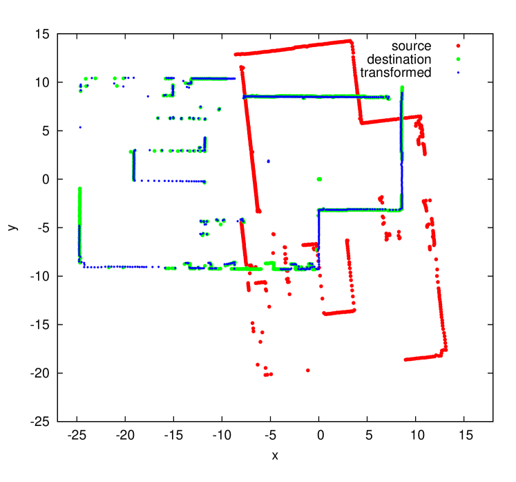
Figure 1: Example of alignment between a source $\mathcal{P}$ (red) and a destination point set $\mathcal{Q}$ (green) with the transformed point set $\mathcal{P}$ (blue).

1.1 Related work

The literature on registration is extensive and includes different formulations for several (sometimes loosely) related problems. The application contexts (computer vision, navigation, etc.) and the formulation of registration (objective function, feature-based or correlation, etc.) result into a variety of works. While there are several classification criteria, the categorization into local and global methods is suitable for thoroughly discussing our contribution w.r.t. the literature.

1.1.1 Local methods

Iterative Closest Point (ICP) [5] is likely the most popular registration algorithm. The estimation is achieved by iteratively alternating the point association and the estimation of the rigid transform that better aligns the associated points. As discussed in section 1, ICP is sensitive to initial estimation and is prone to local minima. Over the years, several variants, like ICP with soft assignment [14], ICP with surface matching [26], affine ICP [11], have been proposed. Generalized Procrustes Analysis (GPA) has also been proposed to simultaneously register multiple point sets in a single optimization step [49, 2]. In some cases, the association among multiple point sets increases the robustness of estimation.

Alternative representations to point sets have been proposed to avoid explicit assessment of correspondences. Biber and Strasser [6] propose the Normal Distributions Transform (NDT) to model the probability of measuring a point as a mixture of normal distributions. Instead of establishing hard associations, NDT estimates the transformation by maximizing the probability density function of the point set matched with the mixture distribution. The approach has been extended to 3D point clouds [32] and, with ICP, is part of standard registration techniques [17]. Other registration techniques are based on GMMs computed on point sets [53, 12, 16].

Several registration algorithms exploit rigidity of isometric transformation for selecting robust and consistent associations. The general procedure operates in two steps. The first step establishes an initial set of putative associations based on geometric criteria (e.g., correspondence to closest neighbor) or similarity of descriptors. The second step filters the outlier associations based on rigidity constraints. RANSAC [13] and its many variants like MLESAC [50] implement this principle through a heuristic random consensus criterion. Coherence point drift (CPD) algorithm [37] represents point sets with a GMM and discriminates outliers by forcing GMM centroids to move coherently as a group. Ma et al. [30] proposed more formally consistent assessment of associations using Vector Field Consensus (VFC). This method solves correspondences by interpolating a vector field between the two point sets. Consensus approach has also been adopted to the non-rigid registration of shapes represented as GMMs [29, 31]. The hypothesize-and-verify approach is often successful in the estimation of associations, but it depends on the initial evaluation of putative correspondences. Moreover, it does not provide any guarantee of optimality of the solution.

1.1.2 Global methods

Global registration methods search the rigid transformation between two point sets on the complete domain of solutions. Heuristic global registration algorithms are based on particle swarm optimization [24], particle filtering [46], simulated annealing [28].

Another category includes the global registration methods that compare features, descriptors and orientation histograms extracted from the original point clouds. Spin Images [22], FPFH [43, 17], SHOT [45] and shape context [4] are descriptors that could be matched according to similarity measure and used for coarse alignment of point clouds. Similar histogram-based methods are applied to rotation estimation of 3D polygon meshes through spherical harmonics representation [7, 34, 33, 23, 3]. All these techniques extend the searching domain and attenuate the problem of local minima, but their computation is prone to failure or achieves extremely coarse estimation. Moreover, the global optimality of the assessed solution is not guaranteed.

In planar registration problem, some effective global methods exploiting specific descriptors of orientation have been proposed. Hough spectrum registration [10] assesses orientation through correlation of histogram measuring point collinearity. The extension of this method to 3D space [9] suffers from observability issues due to symmetry in rotation group. Reyes-Lozano et al. [42] propose to estimate rigid motion using geometric algebra representation of poses and tensor voting. Angular Radon Spectrum [27] estimates the optimal rotation angle that maximizes correlation of collinearity descriptors by performing one-dimensional BnB optimization.

BnB paradigm is the basis for most of global registration methods. Breuel [8] proposes a BnB registration algorithm for several planar shapes in image domain. The shapes are handled by a matchlist containing the shapes to be matched. The bounds are computed using generic geometric properties, which partially exploit pixel discretization. No accurate management of lower bounds is presented. The BnB algorithm in [39, 40] computes the rigid transformation that matches two point sets, under the hypothesis that the set of correspondences is given, although with outliers. The lower bound is derived from the convex relaxation of quaternion components. The point-based formulation is extended also to the registration of points, lines and planes (in principle, any convex model) through similarity transformation. The main limitation lies in the unrealistic assumption that the correspondences between points and convex shapes are known in advance. Brown et al. [BrownWindridgeGuillemaut19] propose the first BnB algorithm for 2D-3D registration, which is the problem of aligning the camera viewpoint given an image to a 3D model of the observed scene. It adopts solutions similar to [52] like a geometric bound and the nested BnB of translation and rotation.

To our knowledge, Go-ICP [52] is the most general algorithm for the estimation of the globally optimal registration. The authors address the formulation for the 3D space domain. The main algorithmic contribution of [52] is the adoption of the uncertainty radius for measuring the distance between a reference point and a matching point transformed according to a 3D isometry belonging to a box. The optimal isometry is estimated by a BnB algorithm, whose lower bound consists of the sum of the minimum distances for each reference point. Note that, to achieve efficiency, Go-ICP algorithm adopts the Euclidean Distance Transformation, which approximates the closest-point distances on a uniform grid and limits the accuracy of optimum value estimation.

1.2 Statement of contribution

The main contribution of this work is the definition of the relaxation bound, that significantly improves the estimation of the lower bound on small sized boxes with respect to the simpler, geometrically based, cheap bound. The superiority of the former bound over the latter is proved theoretically by showing that the relaxation bound is a second-order one (i.e., its error decreases quadratically with the diameter of the box, see Theorem 1), while the cheap bound is first-order (i.e., its error decreases linearly with the diameter of the box, see Proposition 3). Moreover, from the practical point of view, we developed a BnB algorithm that uses the cheap bound for larger boxes and the maximum between the cheap bound and the relaxation bound for smaller ones (and employs a rather efficient queue-based algorithm for their computation). Computational experiments with this BnB algorithm on simulated and real datasets confirm that the addition of the newly proposed relaxation bound strongly enhances the performance of the BnB algorithm. We also stress that the newly proposed relaxation bound has been tested within a specific BnB approach but could be employed in other BnB approaches for the same problem.

Note that in this work we address the planar formulation of the registration problem, since this is a relevant problem with many immediate applications: image registration [15], service and telepresence robots [51, 41], industrial AGV localization and navigation [44, 21]. A natural extension is the one to the 3D formulation of the registration problem. The main ideas of this work and, in particular, the relaxation bound, can indeed be extended to the 3D case. However, the extension is not straightforward and, moreover, the increased complexity of the 3D problem, with the additional degrees of freedom in the rototranslations, makes convergence to the globally optimal solution harder (see also the comments in Section 5.2). Computational tricks like the Euclidean Distance Transformation, adopted in the Go-ICP algorithm, which speeds up computation at the cost of a more limited accuracy in the optimum value estimation, may also apply within the framework of the current work. However, a careful treatment of the 3D case requires many additional considerations which need to be addressed in a separate future work.

1.3 Notation

Given a set $A\subset\mathbb{R}$ with finite cardinality $|A|$, we denote its elements in ascending order as $A_{(1)},A_{(2)},\ldots,A_{(|A|)}$. Given $x,y\in\mathbb{R}$, set $x\wedge y=\min\{x,y\}$. For vectors $x,y\in\mathbb{R}^{n}$, relation $x\leq y$ is intended componentwise. A box $B\subset\mathbb{R}^{n}$ is a set of form $B=\{x\in\mathbb{R}^{n}\ |\ x^{-}\leq x\leq x^{+}\}$ for given $x^{-},x^{+}$, with $x^{-}\leq x^{+}$ ( if $x^{-}\not\leq x^{+}$, then $B$ is empty); moreover, the diameter of $B$ is given by $\sigma(B)=\left\|x^{+}-x^{-}\right\|_{2}$, where $\|\cdot\|_{2}$ denotes the Euclidean norm.

1.4 Paper organization

The rest of the paper is organized as follows. Sections 2 and 3 illustrate the problem formulation and the outline of the BnB algorithm, respectively. Section 4 defines the two lower bounds used within the BnB algorithm. Section 5 describes the complete algorithm. Section 6 presents some technical proofs. Section 7 presents the computational results on simulated point sets and on datasets acquired by laser scanner sensors. Finally, Section 8 gives the concluding remarks.

2 Problem formulation

Consider two sets $\mathcal{P}=\{P_{1},P_{2},\ldots,P_{n}\}$, $\mathcal{Q}=\{Q_{1},Q_{2},\ldots,Q_{m}\}$, with $\mathcal{P},\mathcal{Q}\subset\mathbb{R}^{2}$, representing the coordinates of points acquired with two different measures. Our aim is to find a planar rigid transformation so that the transformed points $\mathcal{P}$ are as close as possible to set $\mathcal{Q}$. Given $x\in\mathbb{R}^{2}$, a generic transformation corresponding to a counter-clockwise rotation by $\theta$ followed by a translation of $z$ can be represented by function $T_{x}(z,\theta):\mathbb{R}^{2}\times\mathbb{S}^{1}\to\mathbb{R}^{2}$, defined as

$$T_{x}(z,\theta)=R(\theta)x+z\,,$$

where $R(\theta)$ is the matrix corresponding to a counter-clockwise rotation by $\theta$, i.e.,

$$R(\theta)=\begin{bmatrix}\cos\theta&-\sin\theta\\ \sin\theta&\cos\theta\end{bmatrix}.$$

Define $f_{x,Q}(z,\theta):\mathbb{R}^{2}\times\mathbb{S}^{1}\to\mathbb{R}$ as

$$f_{x,Q}(z,\theta)=\|T_{x}(z,\theta)-Q\|_{2}^{2}\,,$$

which represents the squared distance between the rototranslation $T_{x}(z,\theta)$ of $x$ and point $Q\in\mathbb{R}^{2}$, and $f_{x}(z,\theta):\mathbb{R}^{2}\times\mathbb{S}^{1}\to\mathbb{R}$ as

$$f_{x}(z,\theta)=\min_{Q\in\mathcal{Q}}\ f_{x,Q}(z,\theta)\,,$$

which represents the squared distance between $T_{x}(z,\theta)$ and set $\mathcal{Q}$, that is the minimum of the distances between $T_{x}(z,\theta)$ and all elements of set $\mathcal{Q}$.
Now, let $p\in\mathbb{N}$, with $1\leq p\leq n$, and consider the following problem.

Problem 1.

$$\min_{z\in\mathbb{R}^{2},\ \theta\in\mathbb{S}^{1},\ S\subset\{1,\ldots,n\}}\ \sum_{i\in S}f_{P_{i}}(z,\theta)$$ (1a)

$$\text{subject to}\quad|S|=p\,.$$ (1b)

Problem 1 consists in finding the rigid transformation that minimizes the sum of a subset of the squared distances between the transformed points $\mathcal{P}$ and set $\mathcal{Q}$. Note that only the smallest $p$ distances are considered in the sum in (1a). In this way, possible outliers (that is, points of $\mathcal{P}$ that do not correspond to any point in $\mathcal{Q}$ or are obtained from erroneous measures) are excluded from the sum defined in (1a). The estimator defined in Problem 1 has a breakdown point of $n-p$, that is, the estimation of the rigid transformation is not compromised if sets $\mathcal{P}$ or $\mathcal{Q}$ contain up to $n-p$ incorrect observations. This is the same principle that is used in Least Trimmed Squares robust regression to reduce the influence of outliers. Problem 1 is non-convex and NP-HARD [35]. In the following, we will present a BnB method for finding its exact solution.

3 Outline of BnB method

Let $B_{0}=\{(z,\theta)\in\mathbb{R}^{2}\times[0,2\pi]\ |\ z^{-}\leq z\leq z^{+}\}$. In this section, we present a BnB algorithm for solving the following restriction of Problem 1 to the initial box $B_{0}$.

Problem 2.

$$\min_{(z,\theta)\in B_{0},\ S\subset\{1,\ldots,n\}}\ \sum_{i\in S}f_{P_{i}}(z,\theta)$$ (2a)

$$\text{subject to}\quad|S|=p\,.$$ (2b)

Let $\mathcal{B}$ denote the set of boxes included in $B_{0}\times[0,2\pi]$ and let $f^{*}:\mathcal{B}\to\mathbb{R}$ be defined as follows:

$$f^{*}(B)=\min_{(z,\theta)\in B,\ S\subset\{1,\ldots,n\}\ \mid\ |S|=p}\quad\sum_{i\in S}f_{P_{i}}(z,\theta).$$

Assume that there exists a function $\phi_{L}:\mathcal{B}\to\mathbb{R}$, such that, $(\forall B\in\mathcal{B})$

$$\phi_{L}(B)\leq f^{*}(B)\,.$$ (3)

We will call any $\phi_{L}$ satisfying (3) a lower bound function. Further, let function $r:\mathcal{B}\to\mathbb{R}^{2}\times[0,2\pi]$ be such that $(\forall B\in\mathcal{B})\ r(B)\in B$. Function $r$ returns a point within box $B$ (in our numerical experiments we always return the center of the box). The optimal solution of Problem 2 can be found with the standard BnB Algorithm 1 adapted from [47, p. 18]. The algorithm uses a binary tree whose nodes are associated to a restriction of Problem 2 to a box, obtained by recursively splitting the initial box $B_{0}$. Input parameter $\epsilon$ represents the maximum relative allowed error on the objective function for the optimal solution and the output variable $x^{*}$ is an approximation of the optimal solution with relative tolerance $\epsilon$. In Algorithm 1, function $\delta:\mathcal{B}\to\mathbb{R}$ is used to define the exploration policy for set $\zeta$. For instance, in a best first search strategy, the node with the lowest lower bound is the next to be processed, so that $\delta(\eta)=-\phi_{L}(\eta)$ (this is also the choice that we made throughout the paper).

Algorithm 1 Main BnB algorithm

Input: $\mathcal{P}$, $\mathcal{Q}$, $B_{0}$: data for Problem 2

$\epsilon$: solution tolerance

Output: $x^{*}$: optimal solution

1. Let $\zeta$ be a list of boxes and initialize $\zeta=\{B_{0}\}$.

2. Set $UB=f(r(B_{0}))$, and $x^{*}=r(B_{0})$.

3. If $\zeta=\varnothing$, stop. Else set $\delta_{\max}=\max\{\delta(\eta)\ |\ \eta\in\zeta\}$.

4. Select a box $\eta\in\zeta$, with $\delta(\eta)=\delta_{\max}$ and split it into two equal smaller sub-boxes $\eta_{1}$, $\eta_{2}$ along the dimension of maximum length.

5. Delete $\eta$ from $\zeta$ and add $\eta_{1}$ and $\eta_{2}$ to $\zeta$.

6. Update $UB=\min\{UB,f(r(\eta_{1})),f(r(\eta_{2}))\}$. If $UB=f(r(\eta_{j}))$ with $j\in\{1,2\}$, set $x^{*}=r(\eta_{j})$.

7. For all $\kappa\in\zeta$, if $\phi_{L}(\kappa)(1+\epsilon)\geq UB$ set $\zeta=\zeta\setminus\kappa$.

8. Return to Step 3.

Note that the choice of the lower bound function $\phi_{L}$ is critical to efficiency of Algorithm 1. The following property on $\phi_{L}$ guarantees that Algorithm 1 converges to a solution of Problem 1, with relative tolerance $\epsilon$.

$$\lim_{\sigma(B)\to 0}\left(\phi_{L}(B)-f^{*}(B)\right)=0\,.$$ (4)

4 Definition of the lower bound function $\phi_{L}$

In the following, we will present two different choices for the lower bound function $\phi_{L}$, denoted by $\phi_{C}$ and $\phi_{R}$. We call the first one the cheap bound, since its computation time is very small and we call the second one the relaxation bound, since it is based on a concave relaxation of Problem 2. We will show that the first bound is well suited for larger boxes, while the second one requires larger computing times but is much more accurate for smaller boxes.

4.1 Cheap bound

Define functions $d_{\min},d_{\max}:\mathcal{B}\times\mathbb{R}^{2}\times\mathbb{R}^{2}\to\mathbb{R}$ as

$$d_{\min}(B,P,Q) =\min_{(z,\theta)\in B}f_{P,Q}(z,\theta)$$

$$d_{\max}(B,P,Q) =\max_{(z,\theta)\in B}f_{P,Q}(z,\theta).$$

If $B=\{(z,\theta)\ |\ z^{-}\leq z\leq z^{+},\theta^{-}\leq\theta\leq\theta^{+}\}$, then $d_{\min}(B,P,Q)$ is the minimum distance between circle arc $\{R(\theta)P\ |\ \theta\in[\theta^{-},\theta^{+}]\}$ and rectangle $\{x\in\mathbb{R}^{2}\ |\ Q-z^{+}\leq x\leq Q-z^{-}\}$, while $d_{\max}(B,P,Q)$ is the maximum distance between the same sets. Details about the computation of these distances will be given in Section 6.1. Functions $d_{\min}$ and $d_{\max}$ can be efficiently computed with the method presented in Section 6. Set $d_{\min}(B,P)=\min_{Q\in\mathcal{Q}}d_{\min}(B,P,Q)$, that is the minimum distance of $P$ with respect to set $\mathcal{Q}$, for $(z,\theta)\in B$. A simple relaxation of Problem 2 is obtained by choosing different parameters $(z,\theta)$ for each point of $\mathcal{P}$, which leads to the following proposition (whose proof is not reported here) and which defines a lower bound closely related to the one presented in [52]).

Proposition 1.

Set

$$\phi_{C}(B)=\sum_{i=1}^{p}\{d_{\min}(B,P)\ |\ P\in\mathcal{P}\}_{(i)}\,,$$ (5)

then $\phi_{C}(B)$ is a lower bound for the solution of Problem 2.

We remind that notation $\{d_{\min}(B,P)\ |\ P\in\mathcal{P}\}_{(i)}$ denotes the $i$-th value of set $\{d_{\min}(B,P)\ |\ P\in\mathcal{P}\}$, orderd in ascending order with respect to its elements, so that (5) corresponds to the sum of the $p$ smallest elements of this set. As the following proposition shows, a brute-force computation of function $\phi_{C}(B)$ can be done in time proportional to the cardinality of set $\mathcal{P}\times\mathcal{Q}$.

Proposition 2.

$\phi_{C}(B)$ can be computed in time $O(nm)$.

Proof.

Quantity $\phi_{C}(B)$ can be obtained by computing all distances $d_{\min}(B,P,Q)$ for all $P\in\mathcal{P}$, which has cardinality $n$, and all $Q\in\mathcal{Q}$, which has cardinality $m$. As we will see in Section 6.1, each $d_{\min}$ and $d_{\max}$ computation requires $O(1)$ computing time. ∎

In Section 5, we will present an algorithm that allows to reduce considerably the number of computations of distances $d_{\min}(B,P,Q)$ required for computing $\phi_{C}$. The following proposition, whose proof is reported in Section 6, shows that $\phi_{C}$ satisfies (4) and that the error $f^{*}(B)-\phi_{C}(B)$ is bounded by a term which is linear with respect to the diameter of $B$.

Proposition 3.

There exists a constant $\Gamma_{C}>0$, dependent on problem data, such that, for any box $B\in\mathcal{B}$,

$$|f^{*}(B)-\phi_{C}(B)|\leq\Gamma_{C}\sigma(B).$$

4.2 Relaxation bound

For $P,Q\in\mathbb{R}^{2}$, define function $f_{P,Q}:\mathbb{R}^{2}\times\mathbb{R}\times\mathbb{R}\to\mathbb{R}$ as

$$f_{P,Q}(z,c,s)=\left\|\begin{bmatrix}c&-s\\ s&c\end{bmatrix}P+z-Q\right\|_{2}^{2}\,.$$

Then, with suitable definition of real constants $c^{-},c^{+},s^{-},s^{+}$, depending on the current box $B$, value $f^{*}(B)$ is equivalent to:

Problem 3.

$$\min_{z\in\mathbb{R}^{2},\ c,s\in\mathbb{R},\ S\subset\{1,\ldots,n\}} \sum_{i\in S}\min_{Q\in\mathcal{Q}}f_{P_{i},Q}(z,c,s)$$ (6a)

subject to $$|S|=p$$ (6b)

$$z^{-}\leq z\leq z^{+}$$ (6c)

$$c^{2}+s^{2}=1$$ (6d)

$$c^{-}\leq c\leq c^{+},\enspace s^{-}\leq s\leq s^{+}\,.$$ (6e)

We relax Problem 3 in the following way:

• We substitute constraints (6d), (6e) with $[c,s]\in\mathcal{A}$, where $\mathcal{A}$ is a convex polygon that contains the circle arc $\{[\cos\theta,\sin\theta]\ |\ \theta^{-}\leq\theta\leq\theta^{+}\}$. In our experiments, we employed an isosceles trapezoid, as illustrated in Figure 3.

• We substitute function $f_{P,Q}$ with an affine underestimator of the same function, namely, a supporting hyperplane of the function at a point within the current box.

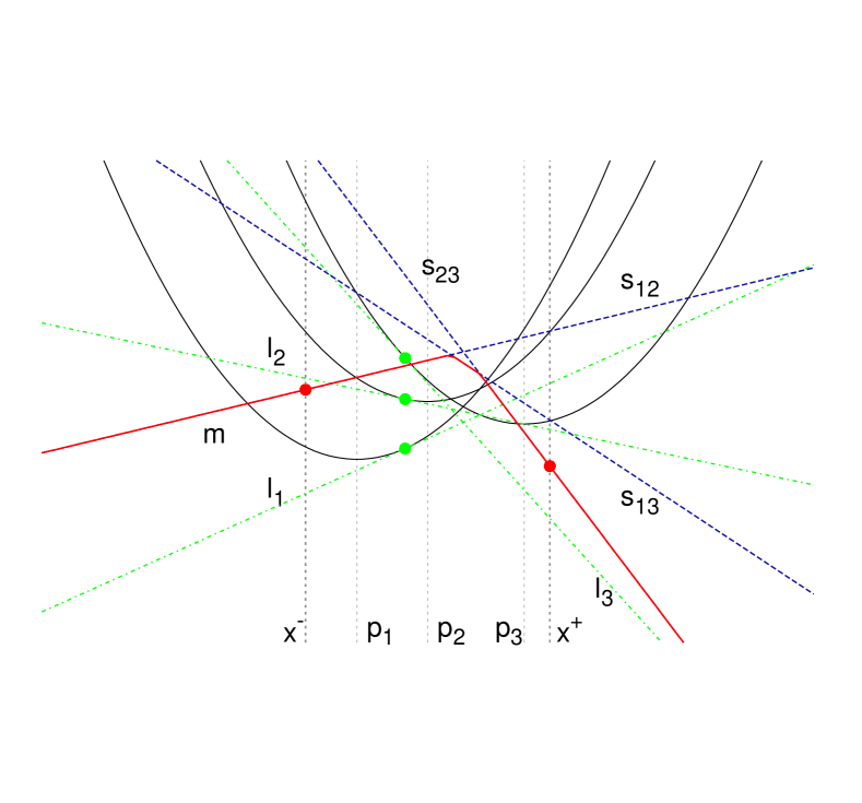
Figure 2: A one dimension example of relaxation bound: the squared distance functions from each given point (black); the linearized distance functions (dash-dotted grey lines) at linearization points (green); the concave objective function of the relaxed problem (red).

As we will show in the following, after these two changes, the modified Problem 3 consists in the minimization of a concave function over a polyhedral domain, so that its minimum is attained at one of the vertices of the domain.

Remark 1.

To give some intuition on the relaxation bound, we consider the following simple problem, where $p_{1},p_{2},p_{3}\in\mathbb{R}$ are assigned positions of three points in a one dimensional domain:

$$\min_{x,S\subset\{1,\ldots,n\}} \sum_{i\in S}((x-p_{i})^{2}+c_{i})$$ (7)

subject to $$|S|=2,\enspace x^{-}\leq x\leq x^{+}\,.$$

Note that the objective function is defined as the minimum of the sum of convex functions. Figure 2 shows the main idea of the relaxation bound applied to this simple example. Namely, green dotted lines $l_{1}$, $l_{2}$, $l_{3}$ represent the supporting hyperplanes of distance functions $(x-p_{i})^{2}+c_{i}$, $i\in\{1,2,3\}$ at the middle point $\frac{x^{-}+x^{+}}{2}$. Blue dotted lines $s_{12}=l_{1}+l_{2}$, $s_{13}=l_{1}+l_{3}$, $s_{23}=l_{2}+l_{3}$ represent the sums of the couples in set $\{l_{1},l_{2},l_{3}\}$, while function $m=\min\{s_{12},s_{13},s_{23}\}$ is a lower bound of the objective function in (7). Note that function $m$ (represented in red) is piecewise-linear concave so that its minimum is achieved at an extremal point of interval $[x^{-},x^{+}]$, that is, $\min_{x^{-}\leq x\leq x^{+}}m(x)=\min\{m(x^{-}),m(x^{+})\}$.

Now, let $\mathcal{A}$ be a convex polygon such that $\{[\cos\theta,\sin\theta]\ |\ \theta^{-}\leq\theta\leq\theta^{+}\}\subset\mathcal{A}$ and let $z_{0}\in\mathbb{R}^{2}$, $c_{0},s_{0}\in\mathbb{R}$ be assigned parameters. Define

$$\hat{f}_{P,Q}(z,c,s)=\nabla f_{P,Q}(z_{0},c_{0},s_{0})[z-z_{0},c-c_{0},s-s_{0}]^{T}+f_{P,Q}(z_{0},c_{0},s_{0})\,,$$

and

$$\hat{f}_{P}(z,c,s)=\min_{Q\in\mathcal{Q}}\hat{f}_{P,Q}(z,c,s)\,.$$

Let us consider the following problem.

Problem 4.

$$\min_{z\in\mathbb{R}^{2},\ c,s\in\mathbb{R},\ S\subset\{1,\ldots,n\}} \sum_{i\in S}\hat{f}_{P_{i}}(z,c,s)$$ (8a)

subject to $$|S|=p$$ (8b)

$$[c,s]\in\mathcal{A},\enspace z^{-}\leq z\leq z^{+}\,,$$ (8c)

We prove the following proposition, which leads to the definition of the relaxation bound.

Proposition 4.

Problem (4) is a relaxation of Problem 3.

Proof.

For any $P\in\mathcal{P}$, $Q\in\mathcal{Q}$, $z\in\mathbb{R}^{2}$, $c,s\in\mathbb{R}$, $\hat{f}_{P,Q}(z,c,s)\leq f_{P,Q}(z,c,s)$, since function $f_{P,Q}$ is convex (being the squared norm of a function linear in $z,c,s$) and $\hat{f}_{P,Q}$ is its supporting hyperplane at point $(z_{0},c_{0},s_{0})$. Hence, for any $z\in\mathbb{R}^{2}$, $c,s\in\mathbb{R}$, $S\subset\{1,\ldots,n\}$, objective function (8a) is not larger than  (6a). Further, conditions (6c) (6d), (6e) imply (8c) by the definition of $\mathcal{A}$ so that the feasible region of Problem 3 is a subset of the feasible region of Problem 4. ∎

Note that, in our experiments, we have always chosen $(z_{0},c_{0},s_{0})$ equal to the center of the current box. As a consequence of Proposition 4, the optimal value of Problem (4) is a lower bound for the optimal value of Problem 3. Thus, next step is to prove that the optimal value of Problem (4) can be efficiently computed. This is stated in the following proposition.

Proposition 5.

Let $V(B)\subset\mathbb{R}^{4}$ be the finite set of vertices of polytope $[z^{-},z^{+}]\times\mathcal{A}$ (we put in evidence the dependency of this set on the current box $B$). Then, the solution of Problem 4 is given by

$$\min_{x\in V(B)}\sum_{i=1}^{p}\{\min_{Q\in\mathcal{Q}}\hat{f}_{P,Q}(x)\ |\ P\in\mathcal{P}\}_{(i)}\,.$$

Proof.

Define function $\tilde{f}:\mathbb{R}^{2}\times\mathbb{R}\times\mathbb{R}\to\mathbb{R}$ as

$$\tilde{f}(z,c,s)=\min_{S\subset\{1,\ldots,n\},|S|=p}\sum_{i\in S}\min_{Q\in\mathcal{Q}}\hat{f}_{P_{i},Q}(z,c,s)\,.$$ (9)

Note that function $\tilde{f}$ is concave. Indeed:

• each function $\hat{f}_{P_{i},Q}$ is linear;

• $\min_{Q\in\mathcal{Q}}\hat{f}_{P_{i},Q}$ is concave since it is the minimum of a finite number of linear functions;

• for each set $S$, we have that $\sum_{i\in S}\min_{Q\in\mathcal{Q}}\hat{f}_{P_{i},Q}$ is concave since it is a sum of concave functions;

• finally, $\tilde{f}$ is concave since it is the minimum of a finite set of concave functions (obtained by all possible subsets $S\subseteq\{1,\ldots,n\}$ with cardinality $p$).

Function $\tilde{f}$ is easily computed by calculating all values of $\min_{Q\in\mathcal{Q}}\hat{f}_{P_{i},Q}(z,c,s)$, for $i\in\{1,\ldots,n\}$ and then summing the $p$ smallest values, namely $\tilde{f}(z,c,s)=\sum_{i=1}^{p}\{\min_{Q\in\mathcal{Q}}\hat{f}_{P,Q}(z,c,s)\ |\ P\in\mathcal{P}\}_{(i)}$. Further, Problem 4 can be reformulated as

Problem 5.

$$\min_{z\in\mathbb{R}^{2},\ c,s\in\mathbb{R}} \tilde{f}(z,c,s)$$ (10a)

subject to $$[c,s]\in\mathcal{A},\enspace z^{-}\leq z\leq z^{+}\,.$$ (10b)

Note that the feasible region is a polytope, while, as already commented, the objective function is concave. Since the minimum of a concave function over a polytope is attained at one of its vertices (for instance, see Property 12, page 58 of [19]), the solution of Problem 5 is obtained by evaluating $\tilde{f}$ at each vertex of $[z^{-},z^{+}]\times\mathcal{A}$ and taking the minimum. ∎

In the following, for a box $B$ we will set

$$\phi_{R}(B)=\min_{x\in V(B)}\sum_{i=1}^{p}\{\min_{Q\in\mathcal{Q}}\hat{f}_{P,Q}(x)\ |\ P\in\mathcal{P}\}_{(i)}\,.$$

As shown in the following proposition, the computation of $\phi_{R}$ has the same time-complexity of $\phi_{C}$.

Proposition 6.

Function $\phi_{R}$ can be computed with time-complexity $O(nm|V(B)|)$.

Proof.

Function $\phi_{R}$ is evaluated by computing $\hat{f}_{P,Q}(z,c,s)$ for all $P\in\mathcal{P}$, $Q\in\mathcal{Q}$ and $(z,c,s)\in V(B)$. ∎

Since one can fix the cardinality of $V(B)$, the time-complexity of the computation of $\phi_{R}$ with respect to the $m$ and $n$ is the same as the cheap bound $\phi_{C}$. However, in practice, computing $\phi_{R}$ takes more time than $\phi_{C}$ because of the computation of the gradient $\hat{f}$ and the necessity of iterating on all vertices of $V(B)$. Anyway, for small boxes, $\phi_{R}$ is a much more accurate lower bound than $\phi_{C}$. This will be theoretically proved in the following theorem. Set $\mathcal{A}$ can be conveniently defined as an isosceles trapezoid as displayed in Figure 3. With this choice, the following theorem, whose proof is given in Section 6, shows that quantity $|f^{*}(B)-\phi_{R}(B)|$ is bounded by a term proportional to $\sigma(B)^{2}$, i.e., the relaxation bound is a second-order one, while we proved in Proposition 3 that the cheap bound is just a first-order one.

Theorem 1.

Under the assumption that convex polygon $\mathcal{A}$ is an isosceles trapezoid (as in Figure 3), there exists a constant $\Gamma_{R}>0$, dependent on problem data, such that, for any box $B\in\mathcal{B}$, with $\theta^{+}-\theta^{-}<\frac{\pi}{2}$,

$$|f^{*}(B)-\phi_{R}(B)|\leq\Gamma_{R}\sigma(B)^{2}.$$

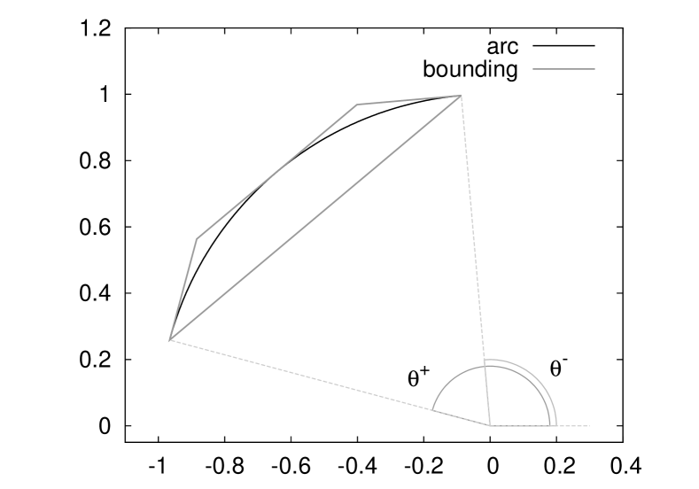
Figure 3: An example of a convex isosceles trapezoid bounding an arc used in the computation of the relaxation bound.

5 Algorithm description

A brute-force evaluation of bound $\phi_{C}$ in (5) requires the computation of all $nm$ distances $d_{\min}(B,P,Q)$ for $P\in\mathcal{P}$ and $Q\in\mathcal{Q}$, for all boxes $B$ encountered during the BnB algorithm. The computation of $\phi_{C}$ can be made more efficient with the following procedure. The main idea is that, if $B^{\prime}\subset B$ is a box obtained by splitting $B$, the evaluation of $\phi_{C}(B^{\prime})$ is simplified by taking into account the information already gained in evaluating $\phi_{C}(B)$. We first need to introduce some operations on ordered lists. Let $\mathcal{L}=(\mathbb{R}\times\{1,\ldots,m\})^{*}$ (where $*$ is the Kleene star [18]) be the set consisting of all ordered pairs of form $(d,i)$. For $L\in\mathcal{L}$, we denote by $\textrm{first}\,(L)$ the first pair of $L$ and by $\textrm{rest}\,(L)$ the list obtained from $L$ by removing its first element. If $L$ is empty, $\textrm{first}\,(L)$ returns $\varnothing_{c}=(-1,0)$, that denotes the empty pair. Further, for any pair $c=(d,i)$, we denote by $\textrm{add}\,(L,c)$, the list obtained by adding $c$ to the list, in such a way that the pairs of $\textrm{add}\,(L,c)$ are ordered in ascending order with respect to the first element of the pair. We associate to each box $B\in\mathcal{B}$ and each $P\in\mathcal{P}$ a list $L_{B,P}\in\mathcal{L}$. The elements $(d,i)$ of $L_{B,P}$ will have the following meaning: $i$ will be the index of a point in set $\mathcal{Q}$ and $d$ will be a lower bound for $d_{\min}(B,P,Q_{i})$. Further, we associate to each $B$ and $P$ a term $U_{B,P}\in\mathbb{R}$, that will represent an upper bound for $\min_{Q\in\mathcal{Q}}d_{\max}(B,P,Q)$. At the beginning, Algorithm 2 is applied to each $P\in\mathcal{P}$, where $B_{0}$ is the box corresponding to the complete domain.

Algorithm 2 Initialization

1:function init($B_{0},P,\mathcal{Q}$)

2:     $U_{B_{0},P}=\infty$

3:     for $j=1$ to $m$ do

4:         $\ell=d_{\min}(B_{0},P,Q_{j})$

5:         $\textsc{add}(L_{B_{0},P},(\ell,j))$

6:         $U_{B_{0},P}=d_{\max}(B_{0},P,Q_{j})\wedge U_{B_{0},P}$

7:     end for

8:     return $L_{B_{0},P}$, $U_{B_{0},P}$

9:end function

Namely, for each $P\in\mathcal{P}$, $L_{B_{0},P}$ is initialized by adding all pairs $\{d_{\min}(B_{0},P,Q_{i})\ |\ i\in\{1,\ldots,m\}\}$, corresponding to all minimum distances between points in $\mathcal{P}$, transformed with all possible transformations corresponding to parameters in $B_{0}$, and the elements of $\mathcal{Q}$. Further $U_{B_{0},P}$ is initialized to $\min\{d_{\max}(B_{0},P,Q_{i})\ |\ i\in\{1,\ldots,m\}\}$, that is the minimum of the upper bounds of the distances between the transformed point $P$ and point set $\mathcal{Q}$.

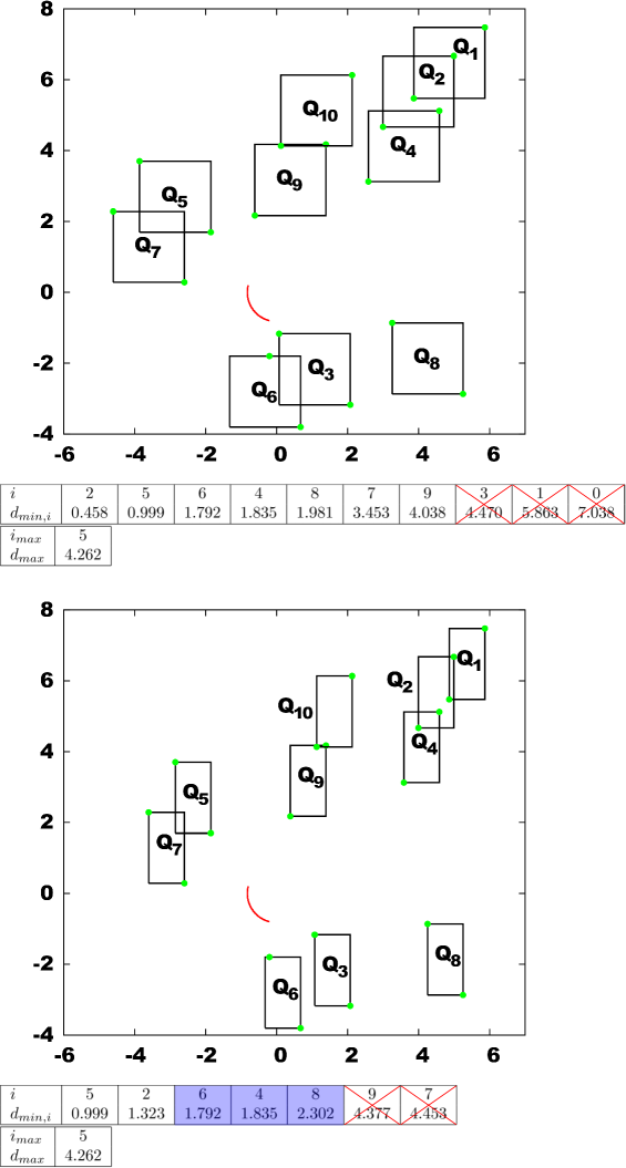
Figure 4: An example illustrating the operations performed in Algorithm 3, for a source point $P$ and a set of destination points $Q_{i}$, with $i\in\{1,\ldots,10\}$. The top figure considers box $B=[0,2]\times[-2,0]\times[\pi/2,\pi]$ and displays arc $\{R(\theta)P\ |\ \theta\in[\pi/2,\pi]\}$ in red and rectangles $\{x\in\mathbb{R}^{2}\ |\ Q_{i}-[2,0]^{T}\leq x\leq Q_{i}-[0,-2]^{T}\}$, with $i\in\{1,\ldots,n\}$. The bottom subfigure represents the same geometrical objects, associated to the child box $B^{\prime}=[0,1]\times[-2,0]\times[\pi/2,\pi]$. The nearest and farthest points from the arc of each rectangle are colored in green. The table below the top figure reports quantities $L_{B,P},U_{B,P}$ and the table below the bottom figure reports $L_{B,P},L_{B^{\prime},P}$.

Then, each time a box $B^{\prime}$ is obtained by splitting a box $B$, Algorithm 3 is applied to $B^{\prime}$, for each $P\in\mathcal{P}$.

Algorithm 3 Lower bound computation

1:function update($B^{\prime}$, $B$, $L_{B,P}$, $U_{B,P}$, $\mathcal{Q}$)

2:     $(d_{\text{old}},i)=\textrm{first}\,(L_{B,P})$

3:     $L_{B,P}=\textrm{rest}\,(L_{B,P})$

4:     $m=d_{\min}(B^{\prime},P,Q_{i})$

5:     $U_{B^{\prime},P}=d_{\max}(B^{\prime},P,Q_{i})$

6:     $\textrm{add}\,L_{B^{\prime},P},(m,i)$

7:     $(d_{\text{old}},i)=\textrm{first}\,(L_{B,P})$

8:     $L_{B,P}=\textrm{rest}\,(L_{B,P})$

9:     while $d_{\text{old}}\leq m$ and $(d_{\text{old}},i)\neq\varnothing_{c}$ do

10:         $d=d_{\min}(B^{\prime},P,Q_{i})$

11:         $m=m\wedge d$

12:         $U_{B^{\prime},P}=U_{B^{\prime},P}\wedge d_{\max}(B^{\prime},P,Q_{i})$

13:         add $(d,i)$ to $L_{B^{\prime},P}$

14:         $(d_{\text{old}},i)=\textrm{first}\,(L_{B,P})$

15:         $L_{B,P}=\textrm{rest}\,(L_{B,P})$

16:     end while

17:     while $U_{B^{\prime},P}>d_{\text{old}}$ and $(d_{\text{old}},i)\neq\varnothing_{c}$ do

18:         add $(d_{\text{old}},i)$ to $L_{B^{\prime},P}$

19:         $(d_{\text{old}},i)=\textrm{first}\,(L_{B,P})$

20:         $L_{B,P}=\textrm{rest}\,(L_{B,P})$

21:     end while

22:     return $L_{B^{\prime},P}$, $U_{B^{\prime},P}$

23:end function

In lines 2–5 the first element $(d_{\text{old}},i)$ of $L_{B,P}$ is removed from $L_{B,P}$ and it is set $m=d_{\min}(B^{\prime},P,Q_{i})$, $U_{B^{\prime},P}=d_{\max}(B^{\prime},P,Q_{i})$. Variables $m$ and $U_{B^{\prime},P}$ represent the minimum values of $d_{\min}(B^{\prime},P,Q_{i})$ and $d_{\max}(B^{\prime},P,Q_{i})$, respectively. Note that, at each iteration, $m$ and $U_{B^{\prime},P}$ will denote the minimum values of $d_{\min}(B^{\prime},P,Q)$ and $d_{\max}(B^{\prime},P,Q)$ among all points $Q$ already processed, respectively. Then, pair $(m,i)$ is added to list $L_{B^{\prime},P}$ associated to the new box $B^{\prime}$, while the next pair $(d_{\text{old}},i)=\textrm{first}\,(L_{B,P})$ is removed from $L_{B,P}$. In lines 9–16, a while cycle is iterated until either the list is empty, in which case all points have been processed, or $d_{\text{old}}\leq m$, in which case the computation of $d_{\min}(B^{\prime},P,Q_{i})$ is not necessary since it would not alter the value of $m$. Note that this is also true for the remaining pairs $(d,i)$ of $L_{B,P}$, since the list is ordered in ascending order of $d$. If the stopping conditions are not fulfilled, quantities $d=d_{\min}(B^{\prime},P,Q_{i})$, $d_{\max}(B^{\prime},P,Q_{i})$ are recomputed (updating $m$ if required) and the updated couples $(d,i)$ are added to $L_{B^{\prime},P}$. Finally, in lines 17– 21 all remaining pairs $(d_{\text{old}},i)$ of $L_{B,P}$ are processed. All pairs such that $d_{\text{old}}<U_{B^{\prime},P}$ are added to $L_{B^{\prime},P}$. Note that pairs $(d_{\text{old}},i)$ that are not added to $L_{B^{\prime},P}$ correspond to points $Q_{i}$ that have a distance to $P$ that is greater than the current value of $U_{B^{\prime},P}$. Hence, they are not added to $L_{B^{\prime},P}$ since they cannot be the element of $\mathcal{Q}$ with minimum distance to $P$ for all transformations belonging to $B^{\prime}$ (or any of its subsets). In this way, list $L_{B^{\prime},P}$ can be smaller than $L_{B,P}$, speeding up all subsequent iterations of the algorithm in boxes obtained by recursively dividing $B^{\prime}$. The following definition states the properties that quantities $L_{B,P}$ and $U_{B,P}$ must satisfy for the correct application of Algorithm 3.

Definition 1.

$L_{B,P}$ and $U_{B,P}$ are consistent if the following conditions are satisfied:

1. For each $(d,i)\in L_{B,P}$, $d_{\min}(B,P,Q_{i})\geq d$;

2. $U_{B,P}\geq\min_{i\in\{1,\ldots,m\}}d_{\max}(B,P,Q_{i})$;

3. For each $i\in\{1,\ldots,n\}$ such that there does not exist any $d\in\mathbb{R}$ such that $(d,i)\in L_{B,P}$, $d_{\min}(B,P,Q_{i})\geq d^{*}$, where $(d^{*},i^{*})=\textrm{first}\,(L_{B,P})$;

4. $d^{*}=\min_{Q\in\mathcal{Q}}d_{\min}(B,P,Q)$, where $(d^{*},j)=\textrm{first}\,(L_{B,P})$.

Remark 2.

In order to better understand the queue update performed by Algorithm 3, we present an example consisting of a source point $P$ and a set of destination points $Q_{i}$, $i\in\{1,\ldots,10\}$, illustrated in Figure 4. Define box $B=[0,2]\times[-2,0]\times[\pi/2,\pi]$. The top subfigure displays arc $\{R(\theta)P\ |\ \theta\in[\pi/2,\pi]\}$, associated to point $P$ and rectangles $\{x\in\mathbb{R}^{2}\ |\ Q_{i}-[2,0]^{T}\leq x\leq Q_{i}-[0,-2]^{T}\}$ associated to points $Q_{i}$, $i\in\{1,\ldots,n\}$. The table below the top subfigure of Figure 4 reports the elements of the sorted queue $L_{B,P}$ and the scalar $U_{B,P}$, for a consistent couple $L_{B,P}$, $U_{B,P}$. Namely, queue $L_{B,P}$ contains couples $(d_{\min,i},i)=(d_{\min}(B,P,Q_{i}),i)$, sorted in ascending order with respect to the the first element, while $U_{B,P}=\min_{i}d_{\max}(B,P,Q_{i})$. The couples $(d_{\min,i},i)$ such that $d_{\min,i}>d_{\max}$ are not present in queue $L_{B,P}$ and are represented as crossed boxes. The bottom subfigure in Figure 4 represents the same geometrical objects, associated to the child box $B^{\prime}=[0,1]\times[-2,0]\times[\pi/2,\pi]$ obtained after splitting $B$ along the first coordinate. The table below the bottom subfigure of Figure 4 shows queue $L_{B^{\prime},P}$ and scalar $U_{B^{\prime},P}$, obtained as the output of Algorithm 3. In particular, the white boxes represent the couples added after the execution of the while cycle in lines 9–16, in which the value of the minimum distance terms $d_{\min,i}$ are updated. The blue boxes represent the couples added in the second while cycle in lines 17–21, in which the values of $d_{\min,i}$ are not updated, while the boxed cells represent the discarded couples among those originally present in $L_{B,P}$.

Note that $L_{B_{0},P}$ and $U_{B_{0},P}$, as defined by the initialization procedure, are consistent. As a consequence, the following proposition proves, by induction, that consistency holds at each iteration of the main BnB algorithm.

Proposition 7.

In Algorithm 3, if input variables $L_{B,P}$ and $U_{B,P}$ are consistent, then output variables $L_{B^{\prime},P}$ and $U_{B^{\prime},P}$ are also consistent.

Proof.

$L_{B^{\prime},P}$ satisfies condition 1). In fact, if pair $(d,i)\in L_{B^{\prime},P}$ is inserted in line 13, then, actually $d=d_{\min}(B^{\prime},P,Q_{i})$. If it is inserted in line 18, $d$ is not recomputed, so that $d\leq d_{\min}(B,P,Q_{i})\leq d_{\min}(B^{\prime},P,Q_{i})$, where the first inequality holds by assumption and the second since $B^{\prime}\subset B$. Moreover, $U_{B^{\prime},P}$ is updated for the last time either in line 5 or line 12. In both cases there exists $i\in\{1,\ldots,n\}$ such that $U_{B^{\prime},P}=d_{\max}(B^{\prime},P,Q_{i})$, so that property 2) holds. To prove 3), assume by contradiction that $d_{\min}(B^{\prime},P,Q_{i})<d^{*}$. This implies that $d_{\min}(B^{\prime},P,Q_{i})\leq d^{*}$, so that $(d,i)$ must have been inserted in $L_{B^{\prime},P}$ in line 13 and, being $d<d^{*}$, $(d^{*},i^{*})\neq\textrm{first}\,(L_{B^{\prime},P})$ (being list $L_{B^{\prime},P}$ ordered) which is a contradiction. Finally, to prove 4), assume by contradiction that there exists $i\in\{1,\ldots,n\}$ such that $d^{*}>d_{\min}(B^{\prime},P,Q_{i})$. By point 3) this implies that $L_{B,P}$ contains a couple of form $(d,i)$. Anyway, no couple of the form $(d,i)$ is added in line 13, because this would imply that $d^{*}\leq d$. This implies that such couple is added in line 18, so that $(d,i)\in L_{B,P}$, that is $(d,i)$ belongs also to the queue of the parent box $B$. Note that quantity $m$ at line 9 is such that $m\geq d^{*}$. This implies that the exit condition for the while-loop in 9 is satisfied for $d_{\text{old}}=d$, contradicting the previously stated fact that no couple of form $(d,i)$ is added to list $L_{B,P}$ in that cycle. ∎

If $\{L_{B,P}\ |\ P\in\mathcal{P}\}$ are consistent bounds for $B$, then $\phi_{C}(B)$ can be computed by summing the first elements of lists $\{L_{B,P}\ |\ P\in\mathcal{P}\}$ as stated in Algorithm 4.

Algorithm 4 Computation of $\phi_{C}$ from $L_{B,P}$

1:function ComputeLBC($\mathcal{P}$, $\{L_{B,P}\ |\ P\in\mathcal{P}\}$,$p$)

2:     $b=0$

3:     for $P\in\mathcal{P}$ do

4:         $(b_{P},i)=\textrm{first}\,(L_{B,P})$

5:     end for

6:     return $\sum_{i=1}^{p}\{b_{P}\ |\ P\in\mathcal{P}\}_{(i)}$

7:end function

Algorithm 5 Computation of $\phi_{R}$ for $B$

1:function ComputeLBR($\mathcal{P}$, $B$, $\{L_{B,P}\ |\ P\in\mathcal{P}\}$, $p$)

2:     Write $B$ as $\{(z,\theta)\ |\ z^{-}\leq z\leq z^{+},\theta^{-}\leq\theta\leq\theta^{+}\}$

3:     Let $\mathcal{A}$ be the vertices of a convex polygon containing arc $\{[\cos\theta,\sin\theta]\ |\ \theta^{-}\leq\theta\leq\theta^{+}\}$

4:     Set $\mathcal{V}=\{z^{-},z^{+}\}\times\mathcal{A}$

5:     $\ell=\infty$

6:     for $v\in\mathcal{V}$ do

7:         Set $X=\varnothing$

8:         for $P\in\mathcal{P}$ do

9:              $m=\infty$

10:              for $(d,i)\in L_{B,P}$ do

11:                  $m=m\wedge\hat{f}(P,Q_{i})$

12:              end for

13:              Set $X=X\cup\{m\}$

14:         end for

15:         $\ell=\ell\wedge\sum_{i=1}^{p}\{X\}_{(i)}$

16:     end for

17:     return $\ell$

18:end function

Algorithm 5 details the computation of the relaxation bound $\phi_{R}$, while the overall implementation of the BnB method is reported in Algorithm 6. Here, $\delta$ is a threshold value for using lower bound function $\phi_{R}$. Namely, $\phi_{C}$ is always computed, since its computational cost is very low, while $\phi_{R}$ is computed only for sufficiently small boxes, where it is more precise than $\phi_{C}$, as a consequence of Theorem 1.

Algorithm 6 Actual implementation of BnB algorithm

Input: $\mathcal{P}$, $\mathcal{Q}$, $R$: data for Problem 2

$\epsilon$: solution tolerance

$\delta$: tolerance for lower bound selection

Output: $x^{*}$: optimal solution

1. Let $\zeta$ be a list of boxes and initialize $\zeta=\{R\}$.

2. For any $P\in Pc$, set $(L_{R,P},U_{R,P})=\textsc{init}(R,P,\mathcal{Q})$

3. Set $UB=f(r(R))$, and $x^{*}=r(R)$.

4. If $\zeta=\varnothing$, stop. Else set $\delta_{\max}=\max\{\delta(\eta)\ |\ \eta\in\zeta\}$.

5. Select a box $\eta\in\zeta$, with $\delta(\eta)=\delta_{\max}$ and split it into two equal smaller sub-boxes $\eta_{1}$, $\eta_{2}$ along the dimension of maximum length.

6. Delete $\eta$ from $\zeta$ and add $\eta_{1}$ and $\eta_{2}$ to $\zeta$.

7. Update $UB=\min\{UB,f(r(\eta_{1})),f(r(\eta_{2}))\}$. If $UB=f(r(\eta_{j}))$ with $j\in\{1,2\}$, set $x^{*}=r(\eta_{j})$.

8. for $j=1,2\ \textbf{do}$

9. for any $P\in\mathcal{P}$, set $(L_{\eta_{j},P},U_{\eta_{j},P})=\textsc{update}(\eta_{j},\eta,P,\mathcal{Q},L_{\eta,P},U_{\eta,P})$

10. $\phi_{C}=\textsc{computeLBC}(\mathcal{P},\{L_{\eta_{j},P}\ |\ P\in\mathcal{P}\})$

11. if  the largest dimension of $\eta$ is lower than $\delta$ then

12. $\phi_{R}=\textsc{computeLBR}(\mathcal{P},\eta_{j},\{L_{\eta_{j},P}\ |\ P\in\mathcal{P}\},p)$

13. else

14. $\phi_{R}=\infty$

15. end if

16. $\phi_{L}(\eta_{j})=\phi_{R}\wedge\phi_{C}$

17. end for

18. For all $\kappa\in\zeta$, if $\phi_{L}(\kappa)(1+\epsilon)\geq UB$ set $\zeta=\zeta\setminus\kappa$.

19. Return to step 3.

5.1 Comparison with the method presented in [52]

At this point, we can compare in more detail our method with the one proposed in [52], which is probably the reference in literature that bears more similarities with our approach, even if [52] considers the 3D registration problem, while we focus on the planar case. In fact, both methods are based on a BnB search on the rigid transformation parameters domain. Moreover, the cheap bound that we defined in this paper is similar to the lower bound estimate defined in [52]. Moreover, with respect to [52], the present paper introduces the following features:

• We introduce the relaxation bound, which is much more accurate than the cheap bound in small boxes (see Proposition 3 and Theorem 1). This second bound allows to close the gap between the upper and lower bound in the BnB algorithm more efficiently than the method presented in [52]. With the numerical experiment presented in Section 7, we will show that the relaxation bound is of fundamental importance for the efficiency of the algorithm.

• We introduce the queue-based algorithm, presented in Section 5, that reduces the number of point-to-point distances to be computed during the BnB recursion. In Section 7, we will show that also this improvement largely affects the overall efficiency of the algorithm.

Moreover, note that in the method presented in [52], the computation of the objective function is based on a precomputed distance transformation on a finite grid. This approach considerably speeds up the computation of the objective function but also introduces a significant error in its evaluation that affects the overall accuracy of the algorithm. In our method, we do not use a precomputed distance transformation, this reduces the speed in the evaluation of the objective function, but does not affect the accuracy of the final result.

5.2 Extension to 3D case

The algorithm can be extended to the 3D case. Note that a 3 dimensional rigid transformation can be described by 6 parameters (3 rotations and 3 translation variables), while 3 parameters are sufficient to represent a rigid planar transformation. The larger dimension requires the development of a very efficient lower bound estimator, in order to avoid evaluating an excessively high number of nodes in the BnB algorithm. One possibility for such a bound consists in the extension of the relaxation bound presented in this paper to the 3D case, using quaternions to parameterize rotations. We are currently working in this direction. Anyway, the 3D case is significantly different from the planar one and is outside the scope of this paper.

6 Proofs

6.1 Computation of $d_{\min}$ and $d_{\max}$

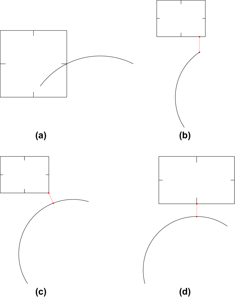
Figure 5: Four configurations of rectangle and arc relevant for the computation of minimum distance between the two geometric shapes: (a) zero distance with intersection; (b) one arc endpoint is the closest arc point to the rectangle; (c) one rectangle vertex is closest to the arc; (d) the closest points are both internal points of a rectangle edge and the arc, respectively.

In order to compute the minimum distance between a circle arc and a rectangle we adopt the following strategy: first, we check whether the arc-rectangle distance is zero. We do that by checking if at least one vertex of the rectangle lies outside the circle to which the arc belongs and if at least one edge of the rectangle has a non-empty intersection with the arc (see Figure 5 (a)). Indeed, if all rectangle vertices lay inside the circle, then the rectangle is contained in the circle and there are no points in common between the arc and the rectangle. If the distance is greater than zero, we have three possibilities: the minimum distance can be attained at an extreme point of the arc (see Figure 5 (b)), at a vertex of the rectangle and an internal point of the arc (see Figure 5 (c)) or at an internal point of an edge of the rectangle and an internal point of the arc (see Figure 5 (d)). Function $d_{\max}$ can be computed by taking the maximum of all the distances between the vertices of the rectangle and the arc.

6.2 Proof of Proposition 3

Given a box $B\in\mathcal{B}$, let $\bar{z},\bar{\theta}$ and $\bar{S}$ be such that $f^{*}(B)=\sum_{i\in\bar{S}}f_{P_{i}}(\bar{z},\bar{\theta})$. Moreover, let $\tilde{S}$ be such that $\sum_{i\in\tilde{S}}d_{\min}(B,P_{i})=\sum_{i=1}^{p}\{d_{\min}(B,P)\ |\ P\in\mathcal{P}\}_{(i)}$. Then, we can write the error as follows

$$\left|f^{*}(B)-\phi_{C}(B)\right|=\left|\sum_{j\in\bar{S}}f_{P_{j}}(\bar{z},\bar{\theta})-\sum_{i\in\tilde{S}}d_{\min}(B,P_{i})\right|\,.$$ (11)

By definition of $f^{*}(B)$, it follows that

$$\sum_{j\in\bar{S}}f_{P_{j}}(\bar{z},\bar{\theta})\leq\sum_{j\in\tilde{S}}f_{P_{j}}(\bar{z},\bar{\theta})\,,$$

so that

$$\left|\sum_{i\in\bar{S}}f_{P_{i}}(\bar{z},\bar{\theta})-\sum_{i\in\tilde{S}}d_{\min}(B,P_{i})\right|\leq\left|\sum_{i\in\tilde{S}}\left(f_{P_{i}}(\bar{z},\bar{\theta})-d_{\min}(B,P_{i})\right)\right|\,.$$ (12)

Now, we can estimate from above each difference in (12) with $\Delta\sigma(B)$, where $\Delta=\max_{i\in\{1,\ldots,p\}}|\nabla f_{P_{i}}|$ and $\nabla f_{P_{i}}$ denotes the gradient of $f_{P_{i}}$, from which we obtain

$$\left|f^{*}(B)-\phi_{C}(B)\right|\leq\sum_{i=1}^{p}\Delta\sigma(B)=p\Delta\sigma(B).$$

6.3 Proof of Theorem 1

Let $B$ be a box in $\mathcal{B}$, if $\theta^{+}-\theta^{-}<\frac{\pi}{2}$, then the maximum distance between the circle arc $\{[\cos\theta,\sin\theta]\ |\ \theta^{-}\leq\theta\leq\theta^{+}\}$ and convex isosceles trapezoid $\mathcal{A}$ is given by $\rho\left(1-\cos\left(\frac{\theta^{+}-\theta^{-}}{2}\right)\right)$, where $\rho$ is the radius of the circle arc. Indeed, under this hypothesis, the pair of points for which the distance arc-trapezoid is maximized is given by the midpoint of the segment joining $(\cos\theta^{-},\sin\theta^{-})$ and $(\cos\theta^{+},\sin\theta^{+})$, that is $\left(\frac{\cos\theta^{+}+\cos\theta^{-}}{2},\frac{\sin\theta^{+}+\sin\theta^{-}}{2}\right)$, and the mid point of the circle arc $\left(\cos\left(\frac{\theta^{+}+\theta^{-}}{2}\right),\sin\left(\frac{\theta^{+}+\theta^{-}}{2}\right)\right)$. We can estimate the error by decomposing it into two components as follows

$$\left|f^{*}(B)-\phi_{R}(B)\right|\leq\left|f^{*}(B)-\phi_{\ell}(B)\right|+\left|\phi_{\ell}(B)-\phi_{R}(B)\right|,$$ (13)

where the first term in (13) represents the linearization error given by $\phi_{\ell}$, in which Problem 3 has been relaxed by substituting $f_{P,Q}$ with a linearization, whilst the second term represents the approximation error due to the substitution of the circle arc with isosceles trapezoid $\mathcal{A}$. Now, by setting

$$\Delta:=\frac{1}{2}\max_{P\in\mathcal{P},Q\in\mathcal{Q}}\max_{|\alpha|=2}\max_{x}|D^{\alpha}f_{P,Q}(x)|,$$

we can estimate from above the first term of (13) using Taylor’s Theorem for multivariate functions (see, for instance, [25]) and the second one applying the consideration on isosceles trapezoid $\mathcal{A}$ we stated earlier, as follows

$$p\Delta\sigma(B)^{2}+p\Delta\rho\left(1-\cos\left(\frac{\theta^{+}-\theta^{-}}{2}\right)\right).$$ (14)

Since $(\forall x\in\mathbb{R})\ 1-\cos(x)\leq\frac{1}{2}x^{2}$, we can rewrite (14) as

$$p\Delta\sigma(B)^{2}+p\Delta\frac{\rho}{8}\left(\theta^{+}-\theta^{-}\right)^{2}.$$ (15)

Now, considering that $\theta^{+}-\theta^{-}\leq\sigma(B)$, we obtain

$$\left|f^{*}(B)-\phi_{R}(B)\right|\leq\left(1+\frac{\rho}{8}\right)p\Delta\sigma(B)^{2}.$$

7 Computational results

This section presents two numerical experiments, the first one is based on random data, the second one on real data acquisitions.

7.1 Randomly generated problems

We generated various random instances of Problem 1. In each case, set $\mathcal{P}=\{P_{1},\ldots,P_{n}\}$ contains $n$ random points with coordinates uniformly distributed in interval $[-10,10]$. Point set $\mathcal{Q}=\{Q_{1},\ldots,Q_{n}\}$ is defined by

$$Q_{i}=T_{P_{i}}(z,\theta)+(1-o_{i})\eta_{i}+o_{i}\gamma_{i},\quad i\in\{1,\ldots,n\}\,.$$

Here, $z\in\mathbb{R}^{2}$ is a random vector whose components are uniformly distributed in $[-10,10]$ and $\theta$ is a random angle obtained from a uniform distribution in $[0,2\pi]$. Vector $[o_{1},\ldots,o_{n}]$ is such that it has $\lceil 0.1n\rceil$ randomly selected components equal to $1$, the others being set to $0$. For $i\in\{1,\ldots,n\}$, $\eta_{i}\in\mathbb{R}$ is a random number obtained from a gaussian distribution centered at $0$ with standard deviation $\sigma$, while $\gamma_{i}$ is uniformly distributed in interval $[-10,10]$. Note that, if $o_{i}=1$, then, with high probability, a very large noise component $\gamma_{i}$ is added to $Q_{i}$, so that $Q_{i}$ becomes an outlier. We set $\epsilon=0.0001$, $p=\lceil 0.8n\rceil$, $\delta=0.1$ and considered different numbers of points $n$, taken from a set of logarithmically spaced values between $10$ and $300$, while $\sigma$ varies in set $\{10^{-4},10^{-3},10^{-2},10^{-1}\}$. We ran these tests on a 2,6 GHz Intel Core i5 CPU, with 8 GB of RAM. We implemented Algorithm 6 in C++ and used Matlab for plotting the results. Figure 6 reports the computation time for different values of $\sigma$ as a function of the number of points $n$. Figure 7 shows the total number of nodes in the BnB algorithm. Note that $\sigma$ has a large effect on both the computation time and the number of nodes. This is related to the fact that larger values of $\sigma$ cause an higher number of local minima in the objective function of Problem 1, that determines a larger number of explored nodes.

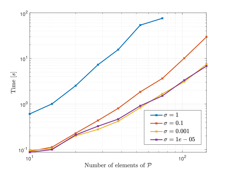
Figure 6: Computation times for randomly generated problems.

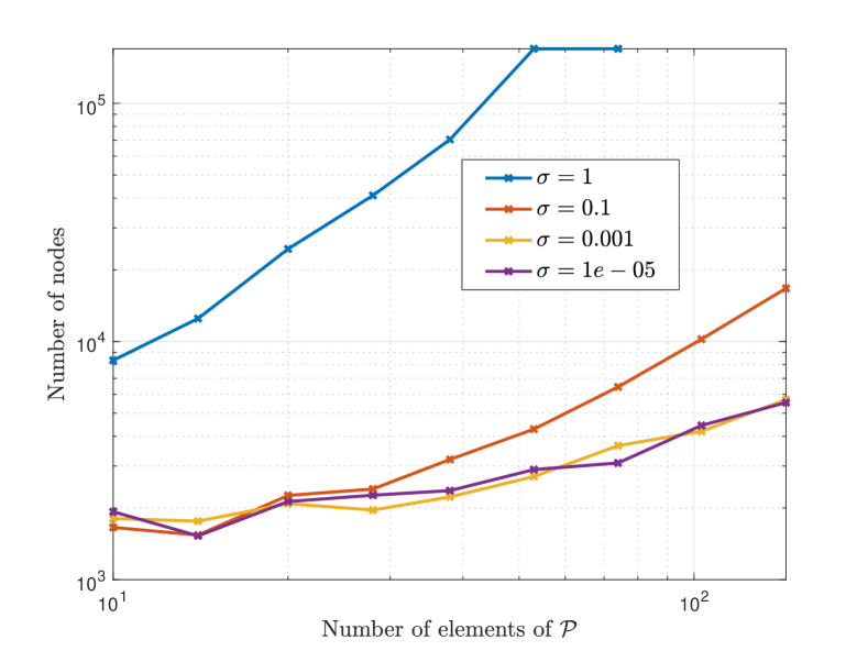
Figure 7: Number of explored nodes for randomly generated problems.

In a second test, we solved random instances of Problem 1, obtained in the same way as in the first test, for different values of the threshold parameter $\delta$ and of standard deviation $\sigma$. Figure 8 reports the computation time for different values of $\sigma$ as a function of $\delta$, while Figure 9 shows the total number of nodes in the BnB algorithm. These figures suggest that the choice of $\delta$ is critical to the efficiency of the algorithm. Namely, if $\delta$ is too small, the relaxation bound is applied only to very small boxes. In this way, the lower bound of the vast majority of boxes is computed only with the cheap bound, that is less efficient (see Proposition 3). In fact, both computational times and total number of nodes increase very much for lower values of $\delta$. On the other hand, if $\delta$ is too large, the relaxation bound is used also for large boxes, for which it gives poor results (since the error grows with the square of the box size, as stated in Theorem 1). Hence, the computation of the relaxation bound for larger boxes is ineffectual and has the only effect of increasing the computation time. Note that the number of nodes is not increased, since, in any case, the cheap bound is computed for all boxes and the overall lower bound for each box is the minimum between the cheap bound and the relaxation bound. Note that these experiments clearly show that the relaxation bound is essential for the efficiency of the algorithm.

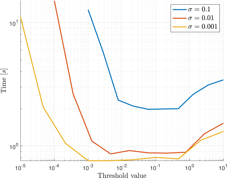
Figure 8: Computation times for randomly generated problems as a function of threshold $\delta$.

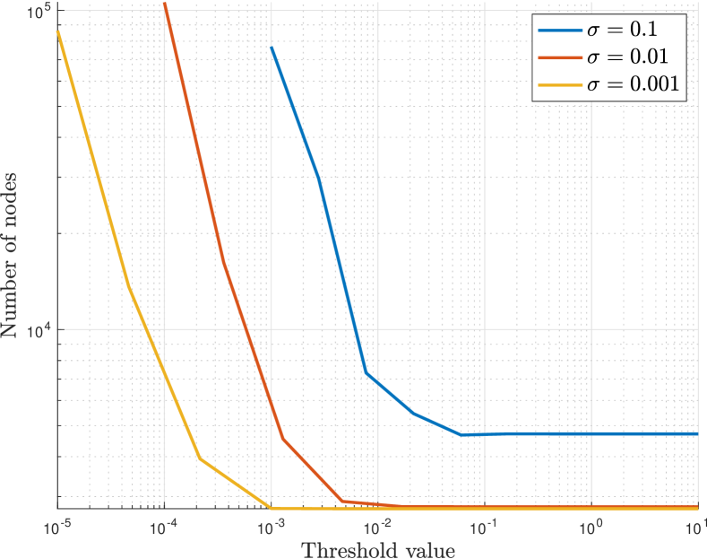
Figure 9: Number of explored nodes for randomly generated problems as a function of threshold $\delta$.

We also performed experiments to assess the impact of the proposed queue management algorithm, presented in Section 5 and Algorithm 6, on computational efficiency. To this end, we solved random instances of Problem 1, obtained in the same way as in the previous tests, for different values of standard deviation $\sigma$, without the use of the queue, computing all items of $L_{B,C}$ from scratch at each iteration, as done in the initialization algorithm. Figures 10 and 11 illustrate the results of these experiments. Note that the execution time of the algorithm with the queue algorithm is significantly lower than the version without the efficient queue management. Note also that we did not perform tests for a number of point $n$ larger than $50$ because the computation time would have been too large.

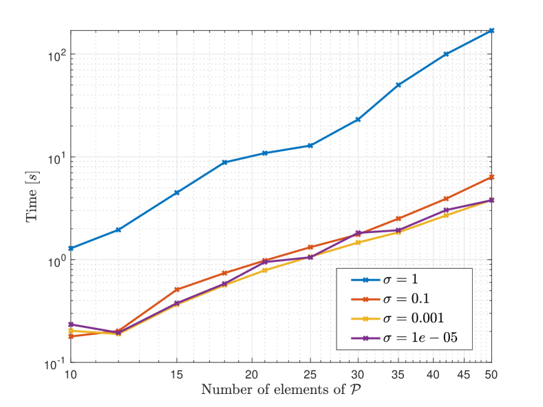
Figure 10: Computation times for randomly generated problems without queue algorithm.

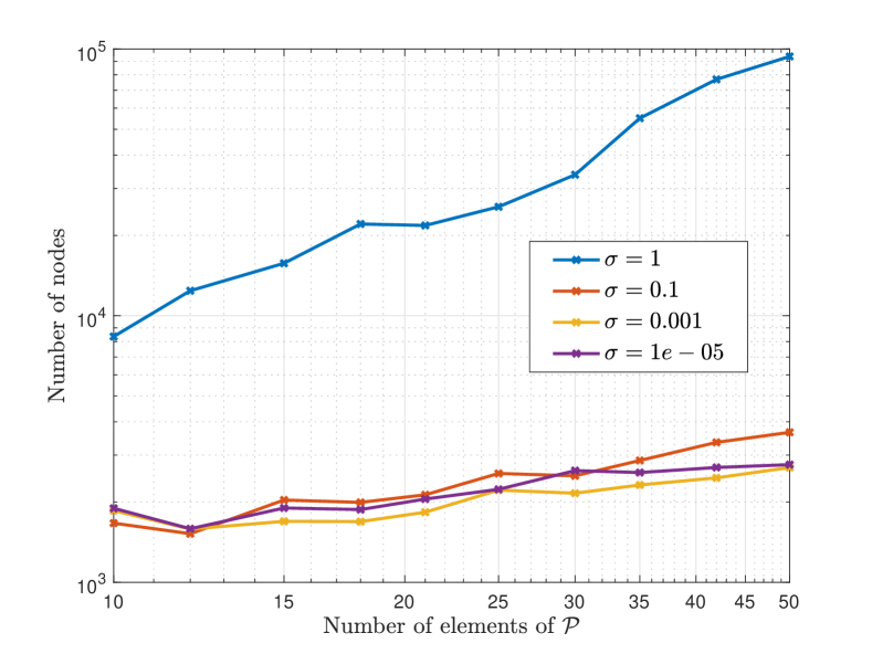
Figure 11: Number of explored nodes for randomly generated problems without queue algorithm.

7.2 Laser scanner data

We obtained some real world data by a lidar sensor Sick NAV350 mounted on an industrial autonomous vehicle. We acquired different point sets, denoted by $\mathcal{L}_{1},\ldots,\mathcal{L}_{S}$, by placing the vehicle at various locations in a warehouse. Each set contains $n=480$ points. It is related to a different vehicle pose (defined by its position and orientation) and each point represents the position of the first obstacle encountered by the lidar laser beam along a given direction. Two such set of points are reported in Figure 1. We considered a set of $S=15$ poses and, for each couple of poses $(i,j)$, we solved Problem 1 with $\mathcal{P}=\mathcal{L}_{i}$ and $\mathcal{Q}=\mathcal{L}_{j}$, computing the solution time $t_{(i,j)}$ and the optimal value $f_{(i,j)}$.

	1	2	3	4	5	6	7	8	9	10	11	12	13
2	40.8
3	36.6	43.0
4	42.7	41.9	38.5
5	41.9	40.1	46.9	49.0
6	43.7	42.1	50.8	41.6	39.2
7	36.9	37.8	37.4	39.3	37.4	31.3
8	63.3	47.7	51.9	58.5	62.8	35.7	44.3
9	39.0	39.2	33.5	40.7	38.7	28.7	30.4	28.6
10	31.3	34.1	31.3	35.1	31.4	25.6	25.7	24.4	24.1
11	30.3	43.4	28.5	33.8	27.5	23.2	23.0	24.0	23.1	23.5
12	27.6	27.2	28.1	29.1	26.9	24.0	26.3	23.4	24.7	24.2	23.9
13	41.6	33.0	36.8	38.1	36.1	31.5	30.6	31.0	32.0	29.6	30.0	28.8
14	29.2	32.1	30.6	28.4	27.8	24.9	28.5	27.9	27.5	28.9	27.9	27.0	29.3

Table 1: Computation times [s] for each pair of poses

	1	2	3	4	5	6	7	8	9	10	11	12	13
2	0.3
3	0.4	0.3
4	0.4	0.3	0.4
5	0.5	0.4	0.5	0.4
6	0.9	0.8	0.9	0.9	0.8
7	1.5	1.4	1.3	1.4	2.3	0.6
8	7.3	4.5	3.5	4.1	8.6	1.2	0.4
9	3.1	2.1	1.7	2.1	4.9	0.8	0.2	0.2
10	1.5	1.4	1.4	1.5	2.8	0.7	0.2	0.3	0.1
11	1.3	1.2	1.3	1.5	2.8	0.7	0.2	0.3	0.1	0.1
12	1.1	1.1	1.2	1.3	2.1	0.6	0.2	0.3	0.2	0.1	0.1
13	1.3	1.3	1.4	1.5	2.6	0.8	0.2	0.4	0.2	0.2	0.1	0.1
14	1.3	1.6	1.8	1.5	2.3	0.5	0.2	0.4	0.2	0.2	0.2	0.2	0.2

Table 2: Minimum for each pair of poses

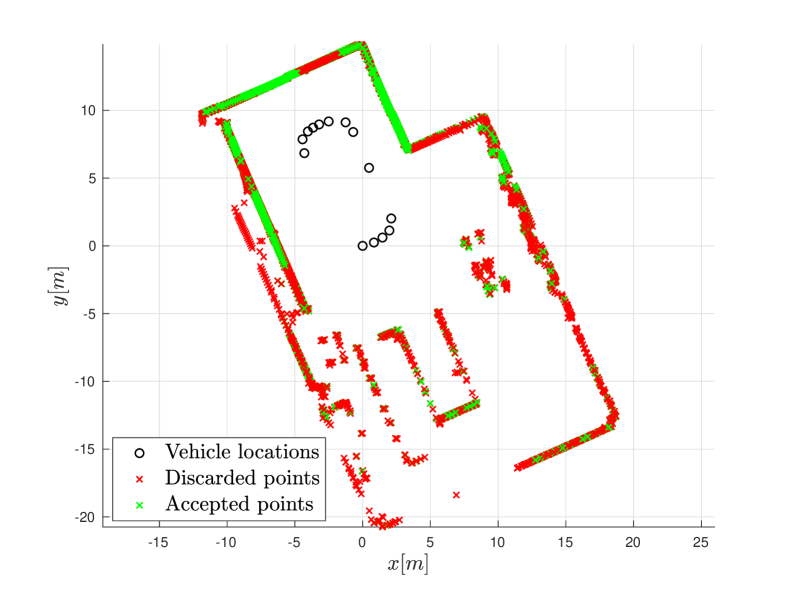
Figure 12: Reconstructed map from laser scanner data.

In our tests, we set $\epsilon=0.0001$, $p=\lceil 0.8n\rceil$ and $\delta=0.1$. We used the same hardware as in the randomly generated tests. The results are reported in Tables 1 and 2. For the sake of representation, we computed the reconstructed vehicle poses and sensed point with respect to the reference frame of the first pose. To this end, we defined an undirected complete graph with nodes $\{1,\ldots,S\}$ and assigned weight $f_{(i,j)}$ to arc $(i,j)$. To define a common reference frame for all poses, we arbitrarily set the pose of $\mathcal{L}_{1}$ at $(0,0)$ with $0$ orientation. Then, we computed the location and orientation of the origin of every set $\mathcal{L}_{i}$, $i\in\{2,\ldots,S\}$, with the following procedure. Let $P$ be the minimum distance path that joins node $i$ to node $1$. We compute the coordinate transformation from the origin of $\mathcal{L}_{i}$ to the origin of $\mathcal{L}_{1}$ by composing the transformations associated to the arcs of $P$. The overall error is minimized since $P$ is the minimum distance path. The results are reported in Figure 12, where the green crosses represent the transformed points that have been included in the sum in (1a), the red crosses represent the points that have not been included in the sum in (1a) (the outliers) and the circles represents the estimated positions of the autonomous vehicle.

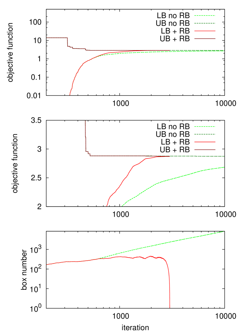
Figure 13: Comparison between BnB registration with or without the relaxation bound (RB). First row: the lower (LB) and upper (UB) bounds of objective error function estimated with (red) or without (green) the RB. Second row: an enlargement of previous plot focused on objective function global minimum. Third row: the number of nodes used by the algorithms with or without the relaxation bound.

We also applied Algorithm 6 to the point sets reported in Figure 1 with and without the use of the relaxation bound. Namely, in a first test we set $\delta=0.8$ and $\epsilon=0.001$, while, in a second test, we changed the value of $\delta$ to $0$, disabling the use of the relaxation bound. In Figure 13, the top and the middle graph (which is a magnification of the top one) report the results of these two tests. In particular, the line denoted by “RB” represent the first test, with $\delta=0.8$ and the line denoted by “no-RB” represents the second one, with the relaxation bound disabled. Note that, with $\delta=0.8$, the lower and upper bounds converge to required relative tolerance $\epsilon=0.001$ after iteration $2123$ whereas, with $\delta=0$, $10000$ iterations are not sufficient. The bottom graph of Figure 13 shows the number of boxes in the queue for the two cases. Note that the number of boxes obtained in the case $\delta=0.8$ is much smaller than in the case $\delta=0$.

8 Conclusions

In this paper, we presented a BnB algorithm for the registration of planar point sets. The algorithm estimates the global minimizer of the objective function given by the sum of distances between each point of the source set to its closest point on the destination set. The main contribution w.r.t. the state-of-the-art global registration lies in the adoption of a novel lower bound, the relaxation bound, which is based on linearized distance and speeds up the convergence of the registration through local linear approximation function exploiting mutual evaluation on the whole point set. Such lower bound is very effective on small boxes, while on larger boxes we adopted the cheap bound, which decomposes the estimation of objective function into the sum of the minimum distances between corresponding points, which considerably improves the performance. This is similar to what already done in [52] but the efficient update and dropping of the candidate closest points is driven by formally guaranteed policies. The correctness and speed of convergence of the proposed bounds as well as the global optimality of the solution are formally proven. Simulation and real datasets acquired with range finders have shown the accuracy and efficiency of the proposed method. In future works, we expect to address the registration problem in 3D space using the same approach to lower bound. The decomposition of error function used in cheap bound and the relaxation bound are general and can be applied to more geometrically complex problems.

References

- [1] A. Aldoma, Z. Marton, F. Tombari, W. Wohlkinger, C. Potthast, B. Zeisl, R. Rusu, S. Gedikli, and M. Vincze. Tutorial: Point Cloud Library: Three-Dimensional Object Recognition and 6 DOF Pose Estimation. IEEE Robotics & Automation Magazine, 19(3):80–91, Sept. 2012.
- [2] J. Aleotti, D. Lodi Rizzini, R. Monica, and S. Caselli. Global Registration of Mid-Range 3D Observations and Short Range Next Best Views. In Proc. of the IEEE/RSJ Int. Conf. on Intelligent Robots and Systems (IROS), pages 3668–3675, 2014.
- [3] S. Althloothi, M. Mahoor, and R. Voyles. A robust method for rotation estimation using spherical harmonics representation. IEEE Trans. on Image Processing, 22(6):2306–2316, June 2013.
- [4] S. Belongie, J. Malik, and J. Puzicha. Shape matching and object recognition using shape contexts. IEEE Trans. on Pattern Analysis and Machine Intelligence, 24, 2002.
- [5] P. Besl and H. Mckay. A method for registration of 3-d shapes. IEEE Trans. Pat. Anal. Mach. Intel, 14(2):239–256, 1992.
- [6] P. Biber and W. Straßer. The normal distributions transform: A new approach to laser scan matching. In Proc. of the IEEE/RSJ Int. Conf. on Intelligent Robots and Systems (IROS), pages 2743–2748, 2003.
- [7] C. Brechbuhler, G. Gerig, and O. Kubler. Parametrization of closed surfaces for 3-d shape description. Computer Vision and Image Understanding, 61(2):154–170, 1995.
- [8] T. Breuel. Implementation Techniques for Geometric Branch-and-bound Matching Methods. Comput. Vis. Image Underst., 90(3):258–294, June 2003.
- [9] A. Censi and S. Carpin. HSM3D: feature-less global 6DOF scan-matching in the Hough/Radon domain. In Proc. of the IEEE Int. Conf. on Robotics & Automation (ICRA), pages 3899–3906, 2009.
- [10] A. Censi, L. Iocchi, and G. Grisetti. Scan Matching in the Hough Domain. In Proc. of the IEEE Int. Conf. on Robotics & Automation (ICRA), 2005.
- [11] S. Du, N. Zheng, S. Ying, and J. Liu. Affine iterative closest point algorithm for point set registration. Pattern Recognition Letters, 31(9):791–799, 2010.
- [12] J. Fan, J. Yang, D. Ai, L. Xia, Y. Zhao, X. Gao, and Y. Wang. Convex hull indexed Gaussian mixture model (CH-GMM) for 3D point set registration. Pattern Recognition, 59:126–141, 2016.
- [13] M. Fischler and R. Bolles. Random Sample Consensus: A Paradigm for Model Fitting with Applications to Image Analysis and Automated Cartography. Commun. ACM, 24(6):381–395, June 1981.
- [14] S. Gold, A. Rangarajan, C.-P. Lu, S. Pappu, and E. Mjolsness. New algorithms for 2D and 3D point matching: Pose estimation and correspondence. Pattern recognition, 31(8):1019–1031, 1998.
- [15] A. Goshtasby and G. C. Stockman. Point pattern matching using convex hull edges. IEEE Transactions on Systems, Man, and Cybernetics, SMC-15(5):631–637, Sep. 1985.
- [16] M. Grogan and R. Dahyot. Shape registration with directional data. Pattern Recognition, 79:452–466, 2018.
- [17] D. Holz, A. Ichim, F. Tombari, R. Rusu, and S. Behnke. Registration with the point cloud library: A modular framework for aligning in 3-d. IEEE Robotics Automation Magazine, 22(4):110–124, Dec 2015.
- [18] J. Hopcroft, R. Motwani, and J. Ullman. Introduction to automata theory, languages, and computation. Addison-Wesley Longman Publishing Co., Inc., Boston, MA, USA, 2006.
- [19] R. Horst and P. Pardalos. Handbook of Global Optimization. Nonconvex Optimization and Its Applications. Springer US, 1995.
- [20] D. Huber and M. Hebert. Fully automatic registration of multiple 3D data sets. Image and vision computing, 21(7):637–650, 2003.
- [21] M. Jaimez, J. Monroy, M. Lopez-Antequera, and J. Gonzalez-Jimenez. Robust planar odometry based on symmetric range flow and multiscan alignment. IEEE Transactions on Robotics, 34(6):1623–1635, Dec 2018.
- [22] A. E. Johnson and M. Hebert. Using spin images for efficient object recognition in cluttered 3D scenes. IEEE Trans. on Pattern Analysis and Machine Intelligence, 21(5):433–449, May 1999.
- [23] M. Kazhdan. An approximate and efficient method for optimal rotation alignment of 3D models. IEEE Trans. on Pattern Analysis and Machine Intelligence, 29(7):1221–1229, 2007.
- [24] M. Khan and I. Nystrom. A modified particle swarm optimization applied in image registration. In 2010 20th International Conference on Pattern Recognition, pages 2302–2305, 2010.
- [25] K. Königsberger. Analysis 2. Springer-Lehrbuch. Springer-Verlag Berlin Heidelberg, 2002.
- [26] Y. Liu. Improving icp with easy implementation for free-form surface matching. Pattern Recognition, 37(2):211–226, 2004.
- [27] D. Lodi Rizzini. Angular Radon Spectrum for Rotation Estimation. Pattern Recognition, 84:182–196, dec 2018.
- [28] J. Luck, C. Little, and W. Hoff. Registration of range data using a hybrid simulated annealing and iterative closest point algorithm. In Proc. of the IEEE Int. Conf. on Robotics & Automation (ICRA), pages 3739–3744, 2000.
- [29] J. Ma, W. Qiu, J. Zhao, Y. Ma, A. Yuille, and Z. Tu. Robust Estimation of Transformation for Non-Rigid Registration. IEEE Transactions on Signal Processing, 63(5):1115–1129, March 2015.
- [30] J. Ma, J. Zhao, J. Tian, A. Yuille, and Z. Tu. Robust Point Matching via Vector Field Consensus. IEEE Transactions on Image Processing, 23(4):1706–1721, April 2014.
- [31] J. Ma, J. Zhao, and A. Yuille. Non-rigid point set registration by preserving global and local structures. IEEE Transactions on Image Processing, 25(1):53–64, Jan 2016.
- [32] M. Magnusson, A. Lilienthal, and T. Duckett. Scan registration for autonomous mining vehicles using 3d-ndt. Journal of Field Robotics, 24(10):803–827, 2007.
- [33] A. Makadia and K. Daniilidis. Rotation recovery from spherical images without correspondences. IEEE Trans. on Pattern Analysis and Machine Intelligence, 28(7):1170–1175, 2006.
- [34] A. Makadia, A. Patterson, and K. Daniilidis. Fully automatic registration of 3d point clouds. In Proc. of IEEE Computer Vision and Pattern Recognition (CVPR), volume 1, pages 1297–1304, 2006.
- [35] D. Mount, N. Netanyahu, C. Piatko, R. Silverman, and A. Wu. On the least trimmed squares estimator. Algorithmica, 69(1):148–183, May 2014.
- [36] R. Mur-Artal, J. Montiel, and J. Tardós. ORB-SLAM: A Versatile and Accurate Monocular SLAM System. IEEE Trans. on Robotics, 31(5):1147–1163, 2015.
- [37] A. Myronenko and X. Song. Point set registration: Coherent point drift. IEEE Trans. on Pattern Analysis and Machine Intelligence, 32(12):2262–2275, Dec 2010.
- [38] A. Nuchter, K. Lingemann, J. Hertzberg, and H. Surmann. 6D SLAM–3D mapping outdoor environments. J. Field Robotics, 21(8–9):699–722, 2006.
- [39] C. Olsson, O. Enqvist, and F. Kahl. A polynomial-time bound for matching and registration with outliers. In IEEE Conf. on Computer Vision and Pattern Recognition, pages 1–8, 2008.
- [40] C. Olsson, F. Kahl, and M. Oskarsson. Branch-and-Bound Methods for Euclidean Registration Problems. IEEE Trans. on Pattern Analysis and Machine Intelligence, 31(5):783–794, May 2009.
- [41] A. Orlandini, A. Kristoffersson, L. Almquist, P. Björkman, A. Cesta, G. Cortellessa, C. Galindo, J. Gonzalez-Jimenez, A. Gustafsson, K.and Kiselev, A. Loutfi, F. Melendez, M. Nilsson, L. Hedman, E. Odontidou, J.-R. Ruiz-Sarmiento, M. Scherlund, L. Tiberio, S. von Rump, and S. Coradeschi. Excite project: A review of forty-two months of robotic telepresence technology evolution. Presence: Teleoperators and Virtual Environments, 25(3):204–221, 2016.
- [42] L. Reyes, G. Medioni, and E. Bayro. Registration of 3D Points Using Geometric Algebra and Tensor Voting. International Journal of Computer Vision, 75(3):351–369, Dec 2007.
- [43] R. Rusu, N. Blodow, and M. Beetz. Fast Point Feature Histograms (FPFH) for 3D registration. In Proc. of the IEEE Int. Conf. on Robotics & Automation (ICRA), pages 3212–3217, 2009.
- [44] L. Sabattini, M. Aikio, P. Beinschob, M. Boehning, E. Cardarelli, V. Digani, A. Krengel, M. Magnani, S. Mandici, F. Oleari, C. Reinke, D. Ronzoni, C. Stimming, R. Varga, A. Vatavu, S. C. Lopez, C. Fantuzzi, A. Mäyrä, S. Nedevschi, C. Secchi, and K. Fuerstenberg. The pan-robots project: Advanced automated guided vehicle systems for industrial logistics. IEEE Robotics Automation Magazine, 25(1):55–64, March 2018.
- [45] S. Salti, F. Tombari, and L. Di Stefano. SHOT: Unique signatures of histograms for surface and texture description. Computer Vision and Image Understanding, 125:251 – 264, 2014.
- [46] J. Sandhu, J. Dambreville, and A. Tannenbaum. Point Set Registration via Particle Filtering and Stochastic Dynamics. IEEE Trans. on Pattern Analysis and Machine Intelligence, 32(8):1459–1473, Aug 2010.
- [47] D. Scholz. Geometric Branch-and-bound Methods and Their Applications. Springer-Verlag New York, 2012.
- [48] J. Serafin and G. Grisetti. Using extended measurements and scene merging for efficient and robust point cloud registration. RAS, 92:91–106, 2017.
- [49] R. Toldo, A. Beinat, and F. Crosilla. Global registration of multiple point clouds embedding the Generalized Procrustes Analysis into an ICP framework. In 5th Int. Symposium 3D Data Processing, Visualization and Transmission (3DPVT2010), 2010.
- [50] P. Torr and A. Zisserman. MLESAC: A New Robust Estimator with Application to Estimating Image Geometry. Computer Vision and Image Understanding, 78(1):138–156, 2000.
- [51] R. Triebel, K. Arras, R. Alami, L. Beyer, S. Breuers, R. Chatila, M. Chetouani, D. Cremers, V. Evers, M. Fiore, H. Hung, O. Ramírez, M. Joosse, H. Khambhaita, T. Kucner, B. Leibe, A. Lilienthal, T. Linder, M. Lohse, M. Magnusson, B. Okal, L. Palmieri, U. Rafi, M. van Rooij, and L. Zhang. SPENCER: A Socially Aware Service Robot for Passenger Guidance and Help in Busy Airports, pages 607–622. Springer International Publishing, 2016.
- [52] J. Yang, H. Li, D. Campbell, and Y. Jia. Go-ICP: A Globally Optimal Solution to 3D ICP Point-Set Registration. IEEE Trans. on Pattern Analysis and Machine Intelligence, 38(11):2241–2254, Nov 2016.
- [53] Y. Yang, S. Ong, and K. Foong. A robust global and local mixture distance based non-rigid point set registration. Pattern Recognition, 48(1):156–173, 2015.