On Particles and Splines in Bounded Domains

Abstract

We propose numerical schemes that enable the application of particle methods for advection problems in general bounded domains. These schemes combine particle fields with Cartesian tensor product splines and a fictitious domain approach. Their implementation only requires a fitted mesh of the domain’s boundary, and not the domain itself, where an unfitted Cartesian grid is used. We establish the stability and consistency of these schemes in $W^{s,p}$-norms, $s\in\mathbb{R}$, $1<p\leq\infty$.

65M12, 65M60, 65M75, 65M85, 65F35, 65D07, 65D10, 65D32

1 Introduction

We begin by introducing a simple toy problem: let $\Omega\subset\mathbb{R}^{\mathrm{D}}$ be an open, bounded Lipschitz domain and let $\mathbf{a}:\bar{\Omega}\times[0,T]\to\mathbb{R}^{\mathrm{D}}$ denote a given, smooth velocity field. Moreover, let us for simplicity assume that $\mathbf{a}$ satisfies $\mathbf{a}\cdot\mathbf{n}=0$ on the boundary $\partial\Omega$, such that we do not need to worry about boundary conditions. We are then interested in solving the initial value problem for the transport equation, i. e., given initial data $u_{0}:\Omega\to\mathbb{R}$, find $u:\Omega\times[0,T)\to\mathbb{R}$ such that:

(1) $$\begin{split}\left\{\begin{aligned} \frac{\partial{u}}{\partial{t}}+(\mathbf{a}\cdot\nabla)u&=0&\text{in }&\Omega\times(0,T),\\ u(\mathbf{x},0)&=u_{0}(\mathbf{x})&\text{on }&\Omega.\end{aligned}\right.\end{split}$$

1.1 Grid-based Schemes

It is well-known that the discretization of this problem with conventional grid-based schemes such as finite differences, volumes, or elements causes a lot of problems when $\mathbf{a}$ is large: for explicit time-stepping schemes the CFL-condition forces one to use tiny time-steps. For the spatial discretization, on the other hand, a common approach to guarantee stability is upwinding. But this comes at the cost of introducing significant amounts of spurious, numerical viscosity: in a numerical solution with $\mathbf{a}\equiv\mathrm{const}$ an initial step function $u_{0}$ quickly turns into a “ridge” of ever decreasing slope. This is the source of many of the difficulties experienced in numerical simulations of turbulent flows and computational fluid dynamics in general. In short, while there certainly are more advanced schemes, it is fair to say that it is very hard to construct grid-based methods that are accurate, stable, and efficient when applied to advection problems.

1.2 Particle Methods

Particle methods like Smoothed Particle Hydrodynamics (SPH) or Vortex Methods (VM) pursue a quite different approach to tackle this problem. Here, the initial data $u_{0}$ is approximated with a special quadrature rule $u_{0,h}$ called particle field. It consists of weights $U_{i}\in\mathbb{R}$ and associated nodes $\mathbf{x}_{i}\in\Omega$, $i=1,\ldots,N$, such that for arbitrary smooth functions $\varphi$ one has:

(2) $$\sum_{i=1}^{N}U_{i}\varphi(\mathbf{x}_{i})\approx\int_{\Omega}{u_{0}\varphi}\,{\mathrm{d}}{\mathbf{x}}.$$

Equivalently, $u_{0,h}$ may be interpreted as a functional: $u_{0,h}=\sum_{i=1}^{N}U_{i}\delta_{\mathbf{x}_{i}}$, where $\delta_{\mathbf{x}_{i}}$ denotes the Dirac $\delta$-functional centered at $\mathbf{x}_{i}$. The reason for such an approximation is as follows. Given such discretized initial data $u_{0,h}\approx u_{0}$, it can be shown that the problem (1) is well-posed and that its unique solution is given by moving the particles with the flow, i. e., by modifying $\mathbf{x}_{i}$ over time according to:

(3) $$\frac{{\mathrm{d}}{\mathbf{x}_{i}}}{{\mathrm{d}}{t}}(t)=\mathbf{a}\bigl{(}\mathbf{x}_{i}(t),t\bigr{)}\qquad i=1,\ldots,N.$$

The fact that this is the exact solution means that apart from the discretization of the initial data, no further error is introduced by the spatial discretization over time. Moreover, for $\mathbf{a}\in L^{\infty}\bigl{(}W^{n,\infty}(\Omega),[0,T]\bigr{)}$, $n\in\mathbb{N}$, one can show that the advection equation is stable in the sense that for all $t\in[0,T]$ the following holds:

(4) $$\|u(t)\|_{W^{s,p}(\Omega)}\lesssim\|u_{0}\|_{W^{s,p}(\Omega)},\qquad-n\leq s\leq n.$$

In this clarity these facts seem to first have been established by Raviart [21] and Cottet [7] in the 1980s. In the context of particle methods the Dirac $\delta$-functional has already been mentioned in 1957 in Appendix II of Evans’ and Harlow’s work on the Particle-in-Cell method; [15] particle methods themselves at least date back to the early 1930s and Rosenhead’s vortex sheet computations. [22] In practice the ODE system (3) is solved numerically using, e. g., a Runge–Kutta scheme and it can be shown that there is no time-step constraint depending on the discretization to guarantee the stability of the method. Simulations with billions of particles have been carried out, [26] and practice has shown that particle schemes have excellent conservation properties and are virtually free of numerical viscosity. In short, particle methods are ideally suited for advection problems.

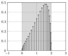
Figure 1: Approximation of the exponential function (blue) on the interval $[0,2]$. On the left: a highly accurate particle approximation. The particle weights, depicted by the arrows’ heights, usually do not correlate well with the local function values. On the right: conventional smoothing of the particle field yields a globally smooth approximation (red) of the target function’s non-smooth zero-extension. This results in poor approximations near its discontinuities at the boundaries. The stabilized $L^{2}$-projection (brown) [17] yields an approximation of a smooth extension. It is not only accurate on the entire interval but also extrapolates well after its ends.

1.3 Particle Methods in Bounded Domains

A particle field $u_{h}$ can only be interpreted as a special quadrature rule; it is important to understand that the $U_{i}$ are weights and not function values. In general, the $U_{i}$ do not give a good picture of the local values $u(\mathbf{x}_{i})$ of the approximated function, much like the quadrature weights from ordinary quadrature rules do not give a good picture of the number 1. This can for example clearly be seen on the left of Fig. 1, where a highly accurate particle approximation of the exponential function on the interval $[0,2]$ is depicted. In reality, however, one is of course interested in function values and a particle approximation is of little practical use. This work therefore focuses on the following two questions:

1. Given a function $u$, how does one construct a particle approximation $u_{h}\approx u$ and what error bounds does it fulfill? Here, $h$ denotes some form of particle spacing and will be defined precisely later. This problem is called particle initialization.

2. Given a particle approximation $u_{h}\approx u$, how does one obtain a function approximation $u_{\sigma}\approx u_{h}$, and what error-bounds does it fulfill? Here, $\sigma$ denotes a smoothing length, which will also be defined precisely later. This problem is called particle regularization.

While in the whole space case these questions are well understood, one of the reasons why particle methods are so rarely used in engineering practice is the difficulty to answer these questions in general bounded domains. In this work we will develop and analyze schemes which aim two solve these problems. Our proposed solutions will only require a mesh of the boundary $\partial\Omega$, not of the domain $\Omega$ itself. Instead, a simple, unfitted Cartesian mesh is used for $\Omega$, which can be obtained easily by a process known in computer graphics as “voxelization”.

The first problem can essentially be solved using quadrature rules. Especially particle regularization, however, is not obvious in the presence of boundaries. The most common approach to the regularization problem is to mollify the particle field with a certain, radially symmetric blob-function $\zeta_{\sigma}$: $u_{\sigma}:=u_{h}\star\zeta_{\sigma}$, where $\sigma$ denotes the radius of the blob’s core. [8, Section 2.3] These blobs are “unaware” of the boundaries and yield poor approximations in their vicinity. In fact, this approach yields globally smooth approximations of the zero-extension of $u$. Unless $u$ itself and its derivatives vanish on $\partial\Omega$, however, this extension is not smooth and cannot be well approximated with a smooth function. This is depicted on the right of Fig. 1. In Particle-in-Cell schemes one uses interpolation formulas to obtain a grid-based approximation of the particle field. In the vicinity of boundaries these formulas need to be specifically adapted to the particular geometry at hand and cannot be used for arbitrary domains. Recently, however, Marichal, Chatelain, and Winckelmans [19] introduced a promising interpolation scheme for general boundaries, but a rigorous error analysis seems unavailable at this time. They also give a review of some other previous approaches and come to the conclusion that “None of the schemes above truly succeeds in the generation of accurate particle – or grid – values around boundaries of arbitrary geometry.”

Recently, we proposed another approach to the regularization problem, which is based on the $L^{2}$-projection and allows a rigorous analysis. [17] First, $C^{\infty}$-smooth finite-element spaces $V_{\sigma}$ on simple uniform Cartesian grids are created, where $\sigma$ denotes the length of the cells. Then a fictitious domain approach is employed and one searches the $L^{2}$-projection of $u$ onto $V_{\sigma}$. In other words one looks for $u_{\sigma}\in V_{\sigma}$ such that

(5) $$\int_{\Omega}{u_{\sigma}v_{\sigma}}\,{\mathrm{d}}{\mathbf{x}}=\int_{\Omega}{uv_{\sigma}}\,{\mathrm{d}}{\mathbf{x}}\qquad\forall v_{\sigma}\in V_{\sigma}.$$

If one is only given a particle approximation $u_{h}\approx u$, the integral on the right is replaced by $\sum_{i=1}^{N}U_{i}v_{\sigma}(\mathbf{x}_{i})$. The addition of a high-order stabilization term then ensures accuracy and stability of the method independent of the position of the boundary $\partial\Omega$ relative to the Cartesian grid. It was established that the resulting $u_{\sigma}$ then approximates a smooth extension of $u$ and is optimal in a certain sense. The result of this approach corresponds to the brown line on the right of Fig. 1, and this figure clearly highlights its accuracy at the boundaries and even beyond.

1.4 Novelty and Main Result

In this work we are going to build on and extend the results from our previous work in several ways. The spaces $V_{\sigma}$ from [17] have the disadvantage that an explicit representation of their basis functions is unavailable. As a first step we are therefore replacing these spaces with Cartesian tensor product splines. Secondly, we extend our error analysis to general $W^{s,p}$-spaces, with $s\in\mathbb{R}$, $1\leq p\leq\infty$. It turns out that splines and particles seem to ideally complement each other and it is also possible to solve the problem of initialization. The main result of this work is summarized in Theorem 4.12. The obtained error bounds closely mirror those given by Raviart [21] for the blob-based regularization in the whole-space case. At the same time, our method works for general bounded domains and is faster: evaluation of the obtained regularized field costs $\mathcal{O}(1)$ operations, compared to $\mathcal{O}(N_{\text{particles}})$ for the blob-based approach.

2 Spaces of Functions and Functionals

In this section we will introduce the function spaces and recall some important results that our analysis will make use of. Throughout this text we will assume that the domain of interest $\Omega\subset\mathbb{R}^{\mathrm{D}}$ is an open, bounded set that satisfies the strong local Lipschitz condition; for short, a Lipschitz domain. This assumption will in particular allow us to make use of the Sobolev embeddings as well as the Stein extension theorem. The symbol $\bigcirc\subset\mathbb{R}^{\mathrm{D}}$ will be used as a placeholder for any bounded Lipschitz domain.

2.1 Sobolev Spaces of Integer Order

As usual, for $n\in\mathbb{N}$, $1\leq p\leq\infty$, the Sobolev spaces $W^{n,p}(\bigcirc)$ are given by:

(6) $$\begin{split}W^{n,p}(\bigcirc)&:=\bigl{\{}f:\bigcirc\to\mathbb{R}\,\big{|}\,\partial^{\alpha}f\in L^{p}(\bigcirc)\ \forall 0\leq|\alpha|\leq n\bigr{\}},\\ \|\cdot\|_{W^{n,p}(\bigcirc)}&:=\biggl{(}\sum_{k=0}^{n}|\cdot|_{W^{k,p}(\bigcirc)}^{p}\biggr{)}^{1/p},\\ |\cdot|_{W^{k,p}(\bigcirc)}&:=\biggl{(}\sum_{|\alpha|=k}\|\partial^{\alpha}(\cdot)\|_{L^{p}(\bigcirc)}^{p}\biggr{)}^{1/p},\end{split}$$

where $W^{0,p}(\bigcirc):=L^{p}(\bigcirc)$, $\alpha\in\mathbb{N}_{0}^{\mathrm{D}}$ denotes a multi-index, $\partial^{\alpha}$ the weak derivative, and the usual modifications for $p=\infty$:

(7) $$\begin{split}\|\cdot\|_{W^{n,\infty}(\bigcirc)}:=\max_{k=0,\ldots,n}|\cdot|_{W^{k,\infty}(\bigcirc)},\\ |\cdot|_{W^{k,\infty}(\bigcirc)}:=\max_{|\alpha|=k}\|\partial^{\alpha}(\cdot)\|_{L^{\infty}(\bigcirc)}.\\ \end{split}$$

Whenever the index $1\leq p\leq\infty$ appears, we define $q$ as its Hölder conjugate such that $\frac{1}{p}+\frac{1}{q}=1$. For $n\neq 0$ we define $W^{-n,p}(\bigcirc):=\bigl{(}W^{n,q}(\bigcirc)\bigr{)}^{\prime}$ to be the normed dual of $W^{n,q}(\bigcirc)$, following the convention of, e. g., Brenner and Scott, [3] but opposed to the convention $W^{-n,p}(\bigcirc)=\bigl{(}W^{n,q}_{0}(\bigcirc)\bigr{)}^{\prime}$ of Adams and Fournier. [1] We define the norm $\|\cdot\|_{W^{-n,p}(\bigcirc)}$ as usual, denoting the duality paring by $\langle\cdot,\cdot\rangle$:

(8) $$\|\cdot\|_{W^{-n,p}(\bigcirc)}:=\sup_{v\in W^{n,q}(\bigcirc)}\frac{\langle\cdot,v\rangle}{\|v\|_{W^{n,q}(\bigcirc)}}.$$

2.2 Sobolev and Besov Spaces of Fractional Order

We will later introduce spline spaces of approximation order $n\in\mathbb{N}$. In terms of integer order Sobolev regularity, these splines however only lie in $W^{n-1,p}$, which in the end would only allow us to prove suboptimal results. We thus introduce intermediate spaces of fractional order, in terms of which the splines possess the necessary amount of regularity.

We define intermediate spaces of fractional order using the “real” interpolation method. [1, Chapter 7] In particular, for $0<\theta<1$, $1\leq p,p^{\prime}\leq\infty$ we define the Besov spaces as $B_{p^{\prime}}^{\theta n,p}(\bigcirc):=\bigl{[}L^{p}(\bigcirc),W^{n,p}(\bigcirc)\bigr{]}_{\theta,p^{\prime}}$. Here $s:=\theta n\in\mathbb{R}_{+}$ measures the smoothness and $1\leq p\leq\infty$ denotes the underlying $L^{p}(\bigcirc)$-space. Varying the secondary index $p^{\prime}$ for fixed values of $s$ and $p$ only results in miniscule changes; bigger values of $p^{\prime}$ result in slightly larger spaces: $B_{p_{1}^{\prime}}^{s,p}(\bigcirc)\hookrightarrow B_{p_{2}^{\prime}}^{s,p}(\bigcirc)$, $1\leq p_{1}^{\prime}\leq p_{2}^{\prime}\leq\infty$. On the other hand, for every $r>s$ and $1\leq p^{\prime}\leq\infty$ we have $B_{p^{\prime}}^{r,p}(\bigcirc)\hookrightarrow B_{1}^{s,p}(\bigcirc)$. For $p\neq\infty$ this definition of Besov spaces is equivalent to the one using appropriate moduli of smoothness. (For $0<p\leq 1$ this has been established by DeVore and Sharpley. [12, Theorem 6.3] For $1<p<\infty$ a proof can be found in Adams’ and Fournier’s book. [1, Theorem 7.47]) For this reason local estimates can be summed up to obtain global ones.

For non-integers $s>0$ we define the Sobolev spaces of fractional order as $W^{s,p}(\bigcirc):=B_{p}^{s,p}(\bigcirc)$. For $p\neq\infty$ these spaces coincide with the Sobolev–Slobodeckij spaces, [12, Theorem 6.7] but unless $p=2$ they differ from the fractional order Sobolev spaces obtained by the “complex” interpolation method as defined by Adams and Fournier. For integer values $s=k$ the Besov spaces $B_{p}^{k,p}(\bigcirc)$ do not coincide with $W^{k,p}(\bigcirc)$, except for the pathological case $p=2$. [1, Section 7.33] However, one always has $B_{1}^{s,p}(\bigcirc)\hookrightarrow W^{s,p}(\bigcirc)\hookrightarrow B_{\infty}^{s,p}(\bigcirc)$. For this reason, we will often first establish our results for all integer values $s=k$ and then conclude by interpolation to the intermediate spaces.

The intermediate spaces with negative index are defined via interpolation, analogously to the positive case: $W^{-\theta n,p}(\bigcirc):=\bigl{[}\bigl{(}L^{q}(\bigcirc)\bigr{)}^{\prime},\bigl{(}W^{n,q}(\bigcirc)\bigr{)}^{\prime}\bigr{]}_{\theta,p}$. For $p\neq 1$, i. e., $q\neq\infty$, it can be shown that they in fact are the dual spaces of the corresponding intermediate spaces with positive index: $W^{-s,p}(\bigcirc)=\bigl{(}W^{s,q}(\bigcirc)\bigr{)}^{\prime}$. [2, Theorem 3.7.1] For this reason, we will sometimes exclude the case $p=1$. In summary, the spaces $W^{s,p}(\bigcirc)$ are defined for all $s\in\mathbb{R}$, $1\leq p\leq\infty$.

2.3 Sobolev Embeddings and Stein Extension

Before moving on to the spline spaces, we recall the Stein extension theorem [25, Chapter VI, Theorem 5]: there exists a linear extension operator $E$ that fulfills $\|Eu\|_{W^{s,p}(\mathbb{R}^{\mathrm{D}})}\lesssim\|u\|_{W^{s,p}(\bigcirc)}$ for all $u\in W^{s,p}(\bigcirc)$, $s\geq 0$, $1\leq p\leq\infty$. We also will use the following variant of the Sobolev embedding theorem: let $s>\tfrac{\mathrm{D}}{p}$ or $s=\mathrm{D}$ if $p=1$. Then $W^{s,p}(\bigcirc)\hookrightarrow C(\bigcirc)$ and $\|u\|_{L^{\infty}(\bigcirc)}\lesssim\|u\|_{W^{s,p}(\bigcirc)}$. Taking into account the secondary index of Besov spaces, for $p\neq\infty$ one can refine the embedding to $B_{1}^{\frac{\mathrm{D}}{p},p}(\bigcirc)\hookrightarrow C(\bigcirc)$. [1, Theorem 4.12 and Theorem 7.34]

2.4 Spline Spaces

The spline spaces will be defined on uniform Cartesian grids, which we introduce first, after which we define the spline spaces and recall some of their properties from approximation theory.

Definition 2.1 (Cartesian Grid and Fictitious Domains).

Let $\sigma>0$ be given. With each $\mathbf{i}\in\mathbb{Z}^{\mathrm{D}}$ we associate a Cartesian grid-point $\mathbf{x_{i}}:=(i_{1}\sigma,i_{2}\sigma,\ldots,i_{\mathrm{D}}\sigma)^{\top}$ and an element $Q_{\mathbf{i}}:=\prod_{d=1}^{\mathrm{D}}\bigl{(}i_{d}\sigma,\,(i_{d}+1)\sigma\bigr{)}$. We define the fictitious domain $\Omega_{\sigma}$ as the union of all elements that intersect the physical domain $\Omega$. Furthermore we define cut and uncut elements $\Omega_{\sigma}^{\Gamma}$ and $\Omega_{\sigma}^{\circ}$, respectively:

(9) $$\begin{split}\Omega_{\sigma}&:=\operatorname{int}\ \bigcup\bigl{\{}\operatorname{clos}{Q_{\mathbf{i}}}\,\bigr{|}\,\operatorname{meas}_{\mathrm{D}}(Q_{\mathbf{i}}\cap\Omega)>0\bigr{\}},\\ \Omega_{\sigma}^{\Gamma}&:=\operatorname{int}\ \bigcup\bigl{\{}\operatorname{clos}{Q_{\mathbf{i}}}\,\bigr{|}\,Q_{\mathbf{i}}\in\Omega_{\sigma}\wedge Q_{\mathbf{i}}\not\subset\Omega\bigr{\}},\\ \Omega_{\sigma}^{\circ}&:=\operatorname{int}\ \bigcup\bigl{\{}\operatorname{clos}{Q_{\mathbf{i}}}\,\bigr{|}\,Q_{\mathbf{i}}\in\Omega_{\sigma}\wedge Q_{\mathbf{i}}\subset\Omega\bigr{\}}.\end{split}$$

The stabilization will make use of the following set of faces near the boundary:

(10) $$\mathcal{F}_{\sigma}:=\{F\text{ is a face of some element }Q_{\mathbf{i}}\in\Omega^{\Gamma}_{\sigma}\text{ and }F\notin\partial\Omega_{\sigma}\}.$$

Here and in what follows we write $Q_{\mathbf{i}}\in\Omega_{\sigma},Q_{\mathbf{i}}\in\Omega_{\sigma}^{\Gamma}$, and $Q_{\mathbf{i}}\in\Omega_{\sigma}^{\circ}$ to refer to the elements these domains are composed of. An illustration of these definitions is given in Fig. 2. We will make use of the following somewhat technical assumption: for every $Q_{\mathbf{i}}\in\Omega_{\sigma}^{\Gamma}$ there exists a finite sequence $(F_{\mathbf{i},1},F_{\mathbf{i},2},\ldots,F_{\mathbf{i},K})\subset\mathcal{F}_{\sigma}$ such that the following conditions are fulfilled: every two subsequent $F_{\mathbf{i},k}$ and $F_{\mathbf{i},k+1}$ are faces of a single element $Q_{\mathbf{j}}$, the number $K$ is bounded independent of $\sigma$ and $\mathbf{i}$, and the last face $F_{\mathbf{i},K}$ belongs to an uncut element $Q_{\mathbf{i}}\in\Omega_{\sigma}^{\circ}$. This assumption means that uncut cells can always be reached from cells in $\Omega_{\sigma}^{\Gamma}$ by crossing a bounded number of faces. For sufficiently small $\sigma$ this condition is often fulfilled with $K=1$; if necessary it can be enforced by moving additional elements from $\Omega_{\sigma}^{\circ}$ to $\Omega_{\sigma}^{\Gamma}$.

Figure 2: An illustration of the fictitious domain approach. The domain $\Omega$ (blue), in this case a circle, may intersect the infinite Cartesian grid in an arbitrary manner. The fictitious domain $\Omega_{\sigma}$ (red) is defined as the union of all intersected cells. The domain $\Omega_{\sigma}^{\circ}$ in this case consists of the four elements entirely lying in $\Omega$. The set of faces $\mathcal{F}_{\sigma}$ is highlighted using bold lines. It can be thought of forming a bridge between $\Omega_{\sigma}^{\circ}$ and the remaining elements in $\Omega_{\sigma}^{\Gamma}$.

Definition 2.2 (Spline Spaces).

Given $n\in\mathbb{N}$ and $1\leq p\leq\infty$, we define the tensor product spline space on the Cartesian grid, equipped with the $L^{p}$-norm:

(11) $$\begin{split}V_{\sigma}^{n,p}(\mathbb{R}^{\mathrm{D}})&:=\bigl{\{}f:\mathbb{R}^{\mathrm{D}}\to\mathbb{R}\,\big{|}\,f|_{Q_{\mathbf{i}}}\in\mathbb{Q}_{n-1},\mathbf{i}\in\mathbb{Z}^{\mathrm{D}}\bigr{\}}\cap C_{0}^{n-2}(\mathbb{R}^{\mathrm{D}}),\\ \|\cdot\|_{V_{\sigma}^{n,p}(\mathbb{R}^{\mathrm{D}})}&:=\|\cdot\|_{L^{p}(\mathbb{R}^{\mathrm{D}})},\end{split}$$

where the symbol $\mathbb{Q}_{n-1}$ refers to the space of polynomials of coordinate-wise degree $n-1$ or less. For $\bigcirc\subset\mathbb{R}^{\mathrm{D}}$, we define $V_{\sigma}^{n,p}(\bigcirc)$ by restriction from $\mathbb{R}^{\mathrm{D}}$ to $\bigcirc$. In analogy to the Sobolev spaces, the normed dual of $V_{\sigma}^{n,q}(\bigcirc)$ will be denoted by $V_{\sigma}^{-n,p}(\bigcirc)$, where $q$ denotes the Hölder conjugate to $p$. Denoting as usual the duality paring by $\langle\cdot,\cdot\rangle$, its norm is thus given by:

(12) $$\|\cdot\|_{V_{\sigma}^{-n,p}(\bigcirc)}:=\sup_{v_{\sigma}\in V_{\sigma}^{n,q}(\bigcirc)}\frac{\langle\cdot,v_{\sigma}\rangle}{\|v_{\sigma}\|_{V_{\sigma}^{n,q}(\bigcirc)}}=\sup_{v_{\sigma}\in V_{\sigma}^{n,q}(\bigcirc)}\frac{\langle\cdot,v_{\sigma}\rangle}{\|v_{\sigma}\|_{L^{q}(\bigcirc)}}.$$

For a fixed bounded domain $\bigcirc$ and fixed values of $\sigma>0$ and $n\in\mathbb{N}$, these spaces of course all have the same topology and are in this sense independent of $p$. In the next sections this notation will prove to be useful, in the other cases the index $p$ will be omitted. It is well-known that for $n\in\mathbb{N}$, $1\leq p\leq\infty$, one has $V_{\sigma}^{n}(\bigcirc)\subset W^{n-1,p}(\bigcirc)$. For $p\neq\infty$ this can be improved to $V_{\sigma}^{n}(\bigcirc)\subset B_{\infty}^{\hat{s},p}(\bigcirc)$, $\hat{s}:=n-1+\tfrac{1}{p}=n-\tfrac{1}{q}$, and furthermore $V_{\sigma}^{n}(\bigcirc)\subset W^{s,p}(\bigcirc)$ for all $0\leq s<\hat{s}$. [11, 12] In particular, the spaces $V_{\sigma}^{n}(\bigcirc)$ are not, but “almost” are embedded in $W^{n,1}(\bigcirc)$.

2.5 Some Properties of Splines

We now introduce some important basic properties of the spline spaces, of which our analysis will make frequent use. For proofs of these result, we refer to Schumaker’s book. [23] The B-splines form a particularly useful basis for the spaces $V_{\sigma}^{n}(\bigcirc)$.

Definition 2.3 (B-Splines).

The cardinal B-splines $b^{n}:\mathbb{R}\to\mathbb{R}$, $n\in\mathbb{N}$, are defined recursively via:

(13) $$b^{1}(x):=\begin{cases}1&x\in[0,1),\\ 0&\text{else},\end{cases}\quad b^{n}(x):=\bigl{(}b^{n-1}\star b^{1}\bigr{)}(x)=\int_{0}^{1}{b^{n-1}(x-y)}\,{\mathrm{d}}{y}.$$

Reusing the symbol $b^{n}$, the corresponding multivariate B-splines are defined coordinate-wise as $b^{n}(\mathbf{x}):=\prod_{d=1}^{\mathrm{D}}b^{n}(x_{d})$. For a given $\sigma>0$, with each Cartesian grid point $\mathbf{x_{i}}$, $\mathbf{i}\in\mathbb{Z}^{\mathrm{D}}$, we associate the shifted and scaled B-spline $b_{\sigma,\mathbf{i}}^{n}(\mathbf{x}):=b^{n}(\tfrac{\mathbf{x}-\mathbf{x}_{i}}{\sigma})$. For a given domain $\bigcirc\subset\mathbb{R}^{\mathrm{D}}$ the corresponding index set is defined as:

(14) $$\Lambda_{\sigma}^{n}(\bigcirc):=\bigl{\{}\mathbf{i}\in\mathbb{Z}^{\mathrm{D}}\ \big{|}\operatorname{meas}_{\mathrm{D}}\bigl{(}\operatorname{supp}{b_{\sigma,\mathbf{i}}^{n}}\cap\bigcirc\bigr{)}>0\bigr{\}}.$$

This basis has many desirable properties, among which are the smallest possible support of its members $\operatorname{supp}b_{\sigma,\mathbf{i}}^{n}=\prod_{d=1}^{\mathrm{D}}[i_{d}\sigma,(i_{d}+n)\sigma]$, their positivity $0\leq b_{\sigma,\boldsymbol{\lambda}}^{n}\leq 1$, the fact that they form a partition of unity $\sum_{\mathbf{i}\in\mathbb{Z}^{\mathrm{D}}}b_{\sigma,\mathbf{i}}^{n}\equiv 1$, and most importantly the norm equivalence that follows.

In what follows, the symbol $\square$ will refer to an arbitrary finite collection of entire cubes from the Cartesian grid, e. g., the domains $\Omega_{\sigma}$, $\Omega_{\sigma}^{\circ}$, or $\Omega_{\sigma}^{\Gamma}$. On such domains one can show some very useful properties, of which we will make frequent use. For proofs of these results and further references we refer the reader to Schumaker’s book. [23]

Lemma 2.4 (Stability of the B-Spline Basis).

Let $\square\subset\mathbb{R}^{\mathrm{D}}$ be a finite collection of entire, uncut cubes $Q_{\mathbf{i}}$ from the Cartesian grid of size $\sigma>0$. Then every function $v_{\sigma}\in V_{\sigma}^{n}(\square)$, $n\in\mathbb{N}$, can be written as

(15) $$u_{\sigma}=\sum_{\boldsymbol{\lambda}\in\Lambda_{\sigma}^{n}(\square)}\mathsf{u}_{\sigma,\boldsymbol{\lambda}}b_{\sigma,\boldsymbol{\lambda}}^{n},$$

with a uniquely determined coefficient vector $\mathsf{u}_{\sigma}=\bigl{(}\mathsf{u}_{\sigma,\boldsymbol{\lambda}}\bigr{)}_{\boldsymbol{\lambda}\in\Lambda_{\sigma}^{n}(\square)}\in\ell^{p}(\Lambda_{\sigma}^{n}(\square))=\mathbb{R}^{\dim V_{\sigma}^{n,p}(\square)}$. The $L^{p}$- and $\ell^{p}$-norms of respectively $u_{\sigma}$ and $\mathsf{u}_{\sigma}$ are equivalent for $1\leq p\leq\infty$:

(16) $$\sigma^{\frac{\mathrm{D}}{p}}\|\mathsf{u}_{\sigma}\|_{\ell^{p}}\lesssim\|u_{\sigma}\|_{L^{p}(\square)}\lesssim\sigma^{\frac{\mathrm{D}}{p}}\|\mathsf{u}_{\sigma}\|_{\ell^{p}}.$$

Lemma 2.5 (Inverse Estimates).

Let $u_{\sigma}\in V_{\sigma}^{n}(\square)$, $n\in\mathbb{N}$. On every element $Q\in\square$ and for all $1\leq p_{1},p_{2}\leq\infty$, $0\leq r\leq s$, the following local inequality holds:

(17) $$\|u_{\sigma}\|_{W^{s,p_{1}}(Q)}\lesssim\sigma^{\frac{\mathrm{D}}{p_{1}}-\frac{\mathrm{D}}{p_{2}}}\sigma^{r-s}\|u_{\sigma}\|_{W^{r,p_{2}}(Q)}.$$

Globally one has for all $1\leq p_{1},p_{2}\leq\infty$, $0\leq s<n-1+\min\{\tfrac{1}{p_{1}},\tfrac{1}{p_{2}}\}$ or $s=n-1$:

(18) $$\|u_{\sigma}\|_{W^{s,p_{1}}(\square)}\lesssim\sigma^{\min\{0,\frac{\mathrm{D}}{p_{1}}-\frac{\mathrm{D}}{p_{2}}\}}\|u_{\sigma}\|_{W^{s,p_{2}}(\square)},$$

and for all $1\leq p\leq\infty$, $0\leq r\leq s<n-1+\tfrac{1}{p}$ or $s=n-1$:

(19) $$\|u_{\sigma}\|_{W^{s,p}(\square)}\lesssim\sigma^{r-s}\|u_{\sigma}\|_{W^{r,p}(\square)}.$$

Lemma 2.6 (Quasi-interpolator).

For every $n\in\mathbb{N}$ there exists a projection operator $P_{\sigma}^{n}:L^{1}(\square)\to V_{\sigma}^{n}(\square)$ called the quasi-interpolator. For all $u\in W^{k,p}(\square)$, $k\in\mathbb{N}_{0}$, $0\leq k\leq n$ this operator fulfills:

(20) $$\|u-P_{\sigma}^{n}u\|_{W^{l,p}(Q)} \lesssim\sigma^{k-l}|u|_{W^{k,p}(\hat{Q})} l\in\{0,\ldots,k\},Q\in\square,$$

(21) $$|P_{\sigma}^{n}u|_{W^{l,p}(Q)} \lesssim\sigma^{k-l}|u|_{W^{k,p}(\hat{Q})} l\in\{k,\ldots,n\},Q\in\square,$$

where $\hat{Q}=\square\cap\bigcup_{\boldsymbol{\lambda}\in\Lambda_{\sigma}^{n}(Q)}\operatorname{supp}b_{\boldsymbol{\lambda},\sigma}^{n}$ is the union of the supports of all the B-splines that do not vanish on $Q$. Moreover, for arbitrary $0\leq r<s\leq n$, $1\leq p_{1}^{\prime},p_{2}^{\prime}\leq\infty$ it holds that:

(22) $$\|u-P_{\sigma}^{n}u\|_{B^{r,p}_{p_{1}^{\prime}}(Q)}\lesssim\sigma^{s-r}\|u\|_{B^{s,p}_{p_{2}^{\prime}}(\hat{Q})}.$$

Remark 2.7.

This result can be improved in the sense that the right hand side of the above inequality (20) only needs to involve “pure” derivatives in the coordinate directions. [10] We will not be able to use this fact, however, because our analysis will rely on the Stein extension theorem, which is formulated for the usual Sobolev spaces involving mixed derivatives.

On domains $\square$ the $L^{2}(\square)$-projection is bounded as an operator from $L^{p}(\square)\to V_{\sigma}^{n,p}(\square)$, $1\leq p\leq\infty$. [13, 9] From this fact and the stability of the B-spline basis it is an easy task to derive the following lemma.

Lemma 2.8.

Every functional $f\in V_{\sigma}^{-n,p}(\square)$, $1\leq p\leq\infty$, has a unique representative $f_{\sigma}\in V_{\sigma}^{n,p}(\square)$ such that:

(23) $$\langle f,v_{\sigma}\rangle=\int_{\square}{f_{\sigma}v_{\sigma}}\,{\mathrm{d}}{x}\qquad\forall v_{\sigma}\in V_{\sigma}^{n,q}(\square).$$

The norms of $f$ and $f_{\sigma}$ are equivalent:

(24) $$\|f_{\sigma}\|_{L^{p}(\square)}\lesssim\|f\|_{V_{\sigma}^{-n,p}(\square)}\leq\|f_{\sigma}\|_{L^{p}(\square)}.$$

3 Particle Initialization

In this section we discuss how to construct particle approximations of spline functions $\tilde{u}_{h}\in V_{h}^{n,p}(\Omega)$. A particle approximation of general functions $u\in L^{p}(\Omega)$ can then be obtained by setting $\tilde{u}_{h}$ to a suitable approximation of $u$.

3.1 Particle Approximations of Splines

As before, let $\Omega\subset\mathbb{R}^{\mathrm{D}}$ denote an open, bounded Lipschitz domain and let $\tilde{u}_{h}\in V_{h}^{n}(\Omega)$, $h>0$, $n>\mathrm{D}$, denote the spline we want to approximate by a particle field. The condition $n>\mathrm{D}$ ensures that $V_{h}^{n}(\Omega)\subset W^{\mathrm{D},p}(\Omega)$ for $1\leq p\leq\infty$, which will simplify the analysis. It is likely that similar results can be obtained for smaller choices of $n$ at the cost of a more technical analysis, but we see no clear benefit from this. For each $\boldsymbol{\lambda}\in\Lambda_{h}^{n}(\Omega)$ we chose quadrature nodes $\mathbf{x}_{\boldsymbol{\lambda},i}\in\Omega\cap\operatorname{supp}b^{n}_{h,\boldsymbol{\lambda}}$ and associated weights $w_{i,\boldsymbol{\lambda}}\in\mathbb{R}$, $i=1,\ldots,N_{\boldsymbol{\lambda}}$, such that:

(25) $$\sum_{i=1}^{N_{\boldsymbol{\lambda}}}|w_{i,\boldsymbol{\lambda}}| \leq C_{\mathrm{Stab}}(nh)^{\mathrm{D}},$$

(26) $$\sum_{i=1}^{N_{\boldsymbol{\lambda}}}w_{i,\boldsymbol{\lambda}}b^{n}_{h,\boldsymbol{\lambda}}(\mathbf{x}_{\boldsymbol{\lambda},i})b^{n}_{h,\boldsymbol{\mu}}(\mathbf{x}_{\boldsymbol{\lambda},i}) = \int_{\Omega}{b^{n}_{h,\boldsymbol{\lambda}}b^{n}_{h,\boldsymbol{\mu}}}\,{\mathrm{d}}{\mathbf{x}}\qquad\forall\boldsymbol{\mu}\in\Lambda_{h}^{n}(\Omega),$$

where $C_{\mathrm{Stab}}\geq 1$ is a user-defined stability constraint.

All that is required to construct such quadrature rules is a mesh of the boundary. For B-splines $b^{n}_{h,\boldsymbol{\lambda}}$ whose support entirely lies in $\Omega$ one can choose standard Gauß–Legendre quadrature rules on each cell $Q\in\operatorname{supp}b^{n}_{h,\boldsymbol{\lambda}}\subset\Omega$. For B-splines with cut support the main difficulty is to compute the integrals on the right for each $\boldsymbol{\mu}$ with $\operatorname{supp}b^{n}_{h,\boldsymbol{\lambda}}\cap\operatorname{supp}b^{n}_{h,\boldsymbol{\mu}}\cap\Omega\neq\emptyset$. This can be done using the boundary mesh: note that the product $b^{n}_{h,\boldsymbol{\lambda}}b^{n}_{h,\boldsymbol{\mu}}$ is again of the form $\prod_{d=1}^{\mathrm{D}}P_{d}(x_{d})$, where the $P_{d}$ are certain one-dimensional, piecewise polynomials with global smoothness $W^{n-1,\infty}$. The ordinary, one-dimensional anti-derivative $\mathcal{P}_{1}(x):=\int_{-\infty}^{x}{P_{1}(x^{\prime})}\,{\mathrm{d}}{x^{\prime}}$ of – for example – $P_{1}$ is known explicitly. We define the vector-valued function $\mathbf{F}(\mathbf{x}):=\left(\mathcal{P}_{1}(x_{1})\prod_{d=2}^{\mathrm{D}}P_{d}(x_{d}),\ 0,\ 0,\ \ldots,\ 0\right)^{\top},$ and note that $\nabla\cdot\mathbf{F}=\prod_{d=1}^{\mathrm{D}}P_{d}(x_{d})=b^{n}_{h,\boldsymbol{\lambda}}b^{n}_{h,\boldsymbol{\mu}}$. The divergence theorem thus allows us to convert the volume integral to a boundary integral:

(27) $$\int_{\Omega}{b^{n}_{h,\boldsymbol{\lambda}}b^{n}_{h,\boldsymbol{\mu}}}\,{\mathrm{d}}{\mathbf{x}}=\int_{\Omega}{\nabla\cdot\mathbf{F}}\,{\mathrm{d}}{\mathbf{x}}=\int_{\partial\Omega}{\mathcal{P}_{1}(x_{1})(\mathbf{e}_{1}\cdot\mathbf{n})\prod_{d=2}^{\mathrm{D}}P_{d}(x_{d})}\,{\mathrm{d}}{S(\mathbf{x})}.$$

On each patch of the boundary mesh the integrand on the right is $W^{n-1,\infty}$-smooth. The integral can thus be efficiently approximated with standard quadrature rules on the boundary mesh. This is similar to the approach of Duczek and Gabbert, [14] who successfully applied it to less smooth shape functions. Once the integrals have been computed, quadrature rules can for example be constructed using the following procedure:

1. Randomly scatter (additional) points $\mathbf{x}_{\boldsymbol{\lambda},i}$ over $\Omega\cap\operatorname{supp}b^{n}_{h,\boldsymbol{\lambda}}$.

2. Solve the following linear programming problem for the unknown weights $w_{\boldsymbol{\lambda},i}$:

   (28) $$\begin{split}\min&\sum_{i=1}^{N_{\boldsymbol{\lambda}}}w_{\boldsymbol{\lambda},i}\\ \sum_{i=1}^{N_{\boldsymbol{\lambda}}}w_{i,\boldsymbol{\lambda}}b^{n}_{h,\boldsymbol{\lambda}}(\mathbf{x}_{\boldsymbol{\lambda},i})b^{n}_{h,\boldsymbol{\mu}}(\mathbf{x}_{\boldsymbol{\lambda},i})&=\int_{\Omega}{b^{n}_{h,\boldsymbol{\lambda}}b^{n}_{h,\boldsymbol{\mu}}}\,{\mathrm{d}}{\mathbf{x}}\qquad\forall\boldsymbol{\mu}\in\Lambda_{h}^{m}(\Omega),\\ w_{\boldsymbol{\lambda},i}\geq 0\end{split}$$

3. If no solution exists that fulfils the stability criterion, go to step 1 and repeat.

Given such quadrature nodes and weights, let us denote by $(c_{\boldsymbol{\lambda}})_{\boldsymbol{\lambda}\in\Lambda_{h}^{n}(\Omega)}$ the B-spline coefficients of $\tilde{u}_{h}$ such that $\tilde{u}_{h}=\sum_{\boldsymbol{\lambda}\in\Lambda_{h}^{n}(\Omega)}c_{\boldsymbol{\lambda}}b^{n}_{h,\boldsymbol{\lambda}}$. We then define the particle approximation $u_{h}$ as follows:

(29) $$u_{h}:=\sum_{\boldsymbol{\lambda}\in\Lambda_{h}^{n}(\Omega)}\sum_{i=1}^{N_{\boldsymbol{\lambda}}}w_{\boldsymbol{\lambda},i}c_{\boldsymbol{\lambda}}b^{n}_{h,\boldsymbol{\lambda}}(\mathbf{x}_{\boldsymbol{\lambda},i})\delta_{\mathbf{x}_{\boldsymbol{\lambda},i}}.$$

3.2 Error Bounds

We will identify the function $\tilde{u}_{h}\in V_{h}^{n,p}(\Omega)$ with the functional

(30) $$\langle\tilde{u}_{h},\varphi\rangle:=\int_{\Omega}{\tilde{u}_{h}\varphi}\,{\mathrm{d}}{\mathbf{x}}\qquad\forall\varphi\in L^{q}(\Omega).$$

The key result of this section is the following theorem.

Theorem 3.1.

The particle approximation $u_{h}$ from (29) fulfills for all $1<p\leq\infty$, $s>\tfrac{\mathrm{D}}{q}$ or $s=\mathrm{D}$ if $q=1$:

(31) $$\|u_{h}\|_{W^{-s,p}(\Omega)}\lesssim h^{\frac{\mathrm{D}}{q}}\|\tilde{u}_{h}\|_{L^{p}(\Omega_{h})}.$$

Moreover, for all $\tfrac{\mathrm{D}}{q}<s\leq n$ or $s=\mathrm{D}$ if $q=1$ the following error bound holds:

(32) $$\|\tilde{u}_{h}-u_{h}\|_{W^{-s,p}(\Omega)}\lesssim h^{s}\|\tilde{u}_{h}\|_{L^{p}(\Omega_{h})}.$$

Proof 3.2.

For arbitrary $\varphi\in W^{s,q}(\Omega)\hookrightarrow C(\Omega)$ it holds by Hölder’s inequality that:

(33) $$\bigl{|}\langle u_{h},\varphi\rangle\bigr{|}=\biggl{|}\sum_{\boldsymbol{\lambda}\in\Lambda_{h}^{n}(\Omega)}\sum_{i=1}^{N_{\boldsymbol{\lambda}}}w_{\boldsymbol{\lambda},i}c_{\boldsymbol{\lambda}}b^{n}_{h,\boldsymbol{\lambda}}(\mathbf{x}_{\boldsymbol{\lambda},i})\varphi(\mathbf{x}_{\boldsymbol{\lambda},i})\biggr{|}\\ \leq\sum_{\boldsymbol{\lambda}\in\Lambda_{h}^{m}(\Omega)}\|\tilde{u}_{h}\|_{L^{\infty}(\operatorname{supp}b^{n}_{h,\boldsymbol{\lambda}})}\|\varphi\|_{L^{\infty}(\operatorname{supp}b^{n}_{h,\boldsymbol{\lambda}}\cap\Omega)}\underbrace{\sum_{i=1}^{N_{\boldsymbol{\lambda}}}|w_{\boldsymbol{\lambda},i}|}_{\lesssim h^{\mathrm{D}}}.$$

Again applying Hölder’s inequality, an inverse inequality for $\tilde{u}_{h}$, and the Sobolev embedding on $\varphi$ this yields with the usual modifications for $p=\infty$:

(34) $$\bigl{|}\langle u_{h},\varphi\rangle\bigr{|}\lesssim h^{\frac{\mathrm{D}}{q}}\biggl{(}\sum_{\boldsymbol{\lambda}\in\Lambda_{h}^{n}(\Omega)}\|\tilde{u}_{h}\|_{L^{p}(\operatorname{supp}b^{n}_{h,\boldsymbol{\lambda}})}^{p}\biggr{)}^{\frac{1}{p}}\biggl{(}\sum_{\boldsymbol{\lambda}\in\Lambda_{h}^{n}(\Omega)}\|\varphi\|_{W^{s,q}(\operatorname{supp}b^{n}_{h,\boldsymbol{\lambda}}\cap\Omega)}^{q}\biggr{)}^{\frac{1}{q}}\\ \lesssim h^{\frac{\mathrm{D}}{q}}\|\tilde{u}_{h}\|_{L^{p}(\Omega_{h})}\|\varphi\|_{W^{s,q}(\Omega)}.$$

This proves (31). For the error bound first note that:

(35) $$\langle\tilde{u}_{h}-u_{h},\varphi\rangle=\underbrace{\langle\tilde{u}_{h}-u_{h},P_{h}^{n}E\varphi\rangle}_{=0}+\langle\tilde{u}_{h},\varphi-P_{h}^{n}E\varphi\rangle-\langle u_{h},\varphi-P_{h}^{n}E\varphi\rangle,$$

where for the second term we have:

(36) $$\langle\tilde{u}_{h},\varphi-P_{h}^{n}E\varphi\rangle\leq\|\tilde{u}_{h}\|_{L^{p}(\Omega_{h})}\|E\varphi-P_{h}^{n}E\varphi\|_{L^{q}(\Omega_{h})}\lesssim h^{s}\|\tilde{u}_{h}\|_{L^{p}(\Omega_{h})}\|\varphi\|_{W^{s,q}(\Omega)}.$$

For the last term we obtain analogous to the proof of (31) that

(37) $$\langle u_{h},\varphi-P_{h}^{n}E\varphi\rangle\lesssim h^{\frac{\mathrm{D}}{q}}\|\tilde{u}_{h}\|_{L^{p}(\Omega_{h})}\biggl{(}\sum_{\boldsymbol{\lambda}\in\Lambda_{h}^{n}(\Omega)}\|E\varphi-P_{h}^{n}E\varphi\|_{L^{\infty}(\operatorname{supp}b^{n}_{h,\boldsymbol{\lambda}})}^{q}\biggr{)}^{\frac{1}{q}}.$$

We now apply the Sobolev embedding for the Besov space $B_{1}^{\frac{\mathrm{D}}{q},q}(\Omega_{h})\hookrightarrow C(\Omega_{h})$ and obtain using Lemma 2.6:

(38) $$\|E\varphi-P_{h}^{n}E\varphi\|_{L^{\infty}(\operatorname{supp}b^{n}_{h,\boldsymbol{\lambda}})}\lesssim\|E\varphi-P_{h}^{n}E\varphi\|_{B^{\frac{\mathrm{D}}{q},q}_{1}(\operatorname{supp}b^{n}_{h,\boldsymbol{\lambda}})}\lesssim h^{s-\frac{\mathrm{D}}{q}}\|E\varphi\|_{W^{s,q}(\widehat{\operatorname{supp}b^{n}_{h,\boldsymbol{\lambda}})}},$$

where $\widehat{\operatorname{supp}b^{n}_{h,\boldsymbol{\lambda}}}=\bigcup_{\boldsymbol{\mu}\in\Lambda_{h}^{n}(\operatorname{supp}b^{n}_{h,\boldsymbol{\lambda}})}\operatorname{supp}b^{n}_{h,\boldsymbol{\mu}}$. Inequality (32) now again follows by a finite overlap argument.

One of the key features of this result is the fact that these estimates only depend on $L^{p}$-norms of the spline $\tilde{u}_{h}$, similar to the results of Cohen and Perthame. [6] Previous estimates have mostly been of the form: $\|u-u_{h}\|_{W^{-s,p}(\Omega)}\lesssim h^{s}\|u\|_{W^{s,p}(\Omega)}$, [8, Theorem A.1.1] suggesting that there might be room for improvement to $h^{2s}$. This is not the case, and we believe that this fact is not well-known in the particle method communities. We therefore recall a theorem of Bakhvalov, [24, Chapter 4, §3] which indicates that these estimates are in fact optimal in terms of convergence order.

Theorem 3.3 (Bakhvalov).

Let $\Omega\subset\mathbb{R}^{\mathrm{D}}$ be a bounded Lipschitz domain, $n\in\mathbb{N}$, $n>\tfrac{\mathrm{D}}{2}$, and let $u\equiv 1$. Let $u_{h,k}=\sum_{i=1}^{N_{k}}U_{i,k}\delta_{\mathbf{x}_{i,k}}$, $k=1,2,\ldots$, denote a sequence of particle approximations of $u$ such that $N_{k}\to\infty$ as $k\to\infty$ and let us define the average particle spacing as $h:=h(k):=\sqrt[\mathrm{D}]{\operatorname{meas}_{\mathrm{D}}(\Omega)/N_{k}}$. Then for every such sequence one has:

(39) $$\|u-u_{h,k}\|_{W^{-n,2}(\Omega)}\gtrsim h^{n}\qquad k\to\infty,$$

with the hidden constant independent of $k$.

Noting that the error bounds only depend on the $L^{p}(\Omega_{h})$-norm of the function $\tilde{u}_{h}$, this constraint can to some extent be bypassed by choosing $n$ very large. This would later allow one to chose the smoothing length $\sigma$ essentially proportional to $h$. On the other hand, the hidden constants in the $\lesssim$-notation get larger as $n$ grows. Furthermore, this approach would require the use of equally smooth trial spaces. The spline spaces that we are going to employ for regularization in the next section only have finite smoothness, however.

4 Particle Regularization

Let $n\in\mathbb{N}$ and $1\leq p\leq\infty$. Our approach will make use of the following operators:

(40) $$A:V_{\sigma}^{n,p}(\Omega_{\sigma})\to V_{\sigma}^{-n,p}(\Omega_{\sigma}),\quad\langle Au_{\sigma},v_{\sigma}\rangle :=\int_{\Omega}{u_{\sigma}v_{\sigma}}\,{\mathrm{d}}{\mathbf{x}},$$

(41) $$J:V_{\sigma}^{n,p}(\Omega_{\sigma})\to V_{\sigma}^{-n,p}(\Omega_{\sigma}),\quad\langle Ju_{\sigma},v_{\sigma}\rangle :=\sigma^{2n-1}\sum_{F\in\mathcal{F}_{\sigma}}\int_{F}{\left\llbracket\frac{\partial{{}^{n-1}u_{\sigma}}}{\partial{\mathbf{n}_{F}^{n-1}}}\right\rrbracket\left\llbracket\frac{\partial{{}^{n-1}v_{\sigma}}}{\partial{\mathbf{n}_{F}^{n-1}}}\right\rrbracket}\,{\mathrm{d}}{S},$$

and $A_{\varepsilon}:=A+\varepsilon J$, where $\varepsilon>0$ denotes a user-defined stabilization parameter. The symbol $\llbracket\cdot\rrbracket$ refers to the jump operator; it is the difference of the one-sided traces on a face $F$. $\mathbf{n}_{F}$ stands for the face’s normal vector, which in our case always coincides with some Cartesian basis vector: $\mathbf{n}_{F}\in\{{\mathbf{e}_{1},\mathbf{e}_{2},\ldots,\mathbf{e}_{\mathrm{D}}}\}$. The stabilization operator $J$ will be called the ghost penalty. [4] The operator $A$ effectively restricts a function from $\Omega_{\sigma}$ to $\Omega$. We will establish that its stabilized version $A_{\varepsilon}$ is invertible, yielding the approximate extension operator $A_{\varepsilon}^{-1}$.

4.1 Continuity and Consistency

For $\varepsilon=0$ the approximate extension operator $A_{0}^{-1}$ is the $L^{2}(\Omega)$-projection onto $V_{\sigma}^{n}(\Omega_{\sigma})$. For $\varepsilon>0$, however, $A_{\varepsilon}^{-1}$ ceases to be a projection, but the difference to $A_{0}^{-1}$ is small; a fact we will call consistency. The main difference to previous analyses of the ghost penalty operator is that we consider results in $L^{p}$-spaces for $p\neq 2$.

Lemma 4.1.

The ghost-penalty operator $J$ is continuous. In other words, for all $u_{\sigma}\in V_{\sigma}^{n,p}(\Omega_{\sigma})$, $n\in\mathbb{N}$, $1\leq p\leq\infty$, it holds that:

(42) $$\|Ju_{\sigma}\|_{V^{-n,p}(\Omega_{\sigma})}\lesssim\|u_{\sigma}\|_{L^{p}(\Omega_{\sigma})}.$$

Moreover, for any $u\in W^{s,p}(\Omega_{\sigma})$, $0\leq s\leq n$, the quasi-interpolant $P_{\sigma}^{n}u$ of $u$ fulfils:

(43) $$\|JP_{\sigma}^{n}u\|_{V^{-n,p}(\Omega_{\sigma})}\lesssim\sigma^{s}\|u\|_{W^{s,p}(\Omega_{\sigma})}.$$

Proof 4.2.

For arbitrary $u_{\sigma}\in V_{\sigma}^{n,p}(\Omega_{\sigma})$ and $v_{\sigma}\in V_{\sigma}^{n,q}(\Omega_{\sigma})$ we obtain by repeatedly using Hölder’s and the triangular inequality:

(44) $$\bigl{|}\bigl{\langle}Ju_{\sigma},v_{\sigma}\bigr{\rangle}\bigr{|}=\sigma^{2n-1}\left|\sum_{F\in\mathcal{F}_{\sigma}}\int_{F}{\left\llbracket\frac{\partial{{}^{n-1}u_{\sigma}}}{\partial{\mathbf{n}_{F}^{n-1}}}\right\rrbracket\left\llbracket\frac{\partial{{}^{n-1}v_{\sigma}}}{\partial{\mathbf{n}_{F}^{n-1}}}\right\rrbracket}\,{\mathrm{d}}{S}\right|\\ \leq\sigma^{2n-1}\left(\sum_{F\in\mathcal{F}_{\sigma}}\left\|\left\llbracket\frac{\partial{{}^{n-1}u_{\sigma}}}{\partial{\mathbf{n}_{F}^{n-1}}}\right\rrbracket\right\|_{L^{p}(F)}^{p}\right)^{\frac{1}{p}}\left(\sum_{F\in\mathcal{F}_{\sigma}}\left\|\left\llbracket\frac{\partial{{}^{n-1}v_{\sigma}}}{\partial{\mathbf{n}_{F}^{n-1}}}\right\rrbracket\right\|_{L^{q}(F)}^{q}\right)^{\frac{1}{q}}$$

with the usual modifications for $p=\infty$ or $q=\infty$. For arbitrary $w\in W^{1,p}(Q)$, $1\leq p\leq\infty$, $Q\in\Omega_{\sigma}$ an arbitrary cube from the Cartesian grid, we have the trace estimate $\|w\|_{L^{p}(\partial Q)}\lesssim\|w\|_{L^{p}(Q)}^{\frac{1}{q}}\|w\|_{W^{1,p}(Q)}^{\frac{1}{p}}$. [3, Lemma (1.6.6)] Together with an inverse estimate this leads to:

(45) $$\left\|\left\llbracket\frac{\partial{{}^{n-1}u_{\sigma}}}{\partial{\mathbf{n}_{F}^{n-1}}}\right\rrbracket\right\|_{L^{p}(F)} \lesssim\|u_{\sigma}\|_{W^{n-1,p}(Q(F))}^{\frac{1}{q}}\|u_{\sigma}\|_{W^{n,p}(Q(F))}^{\frac{1}{p}}\stackrel{{\scriptstyle\eqref{eqn:localinverseineq}}}{{\lesssim}}\sigma^{-\frac{1}{p}}\|u_{\sigma}\|_{W^{n-1,p}(Q(F))},$$

(46) $$\left\|\left\llbracket\frac{\partial{{}^{n-1}v_{\sigma}}}{\partial{\mathbf{n}_{F}^{n-1}}}\right\rrbracket\right\|_{L^{q}(F)} \lesssim\|v_{\sigma}\|_{W^{n-1,q}(Q(F))}^{\frac{1}{p}}\|v_{\sigma}\|_{W^{n,q}(Q(F))}^{\frac{1}{q}}\stackrel{{\scriptstyle\eqref{eqn:localinverseineq}}}{{\lesssim}}\sigma^{-\frac{1}{q}}\|u_{\sigma}\|_{W^{n-1,q}(Q(F))}.$$

The $W^{n,p}$- and $W^{n,q}$-norms in the intermediate step are to be interpreted in the “broken”, element-wise sense and $Q(F)$ denotes the two elements that $F$ is a face of. Thus, using a finite-overlap argument, one obtains together with another application of the inverse estimates: $\bigl{|}\bigl{\langle}Ju_{\sigma},v_{\sigma}\bigr{\rangle}\bigr{|}\lesssim\sigma^{2n-2}\|u_{\sigma}\|_{W^{n-1,p}(\Omega_{\sigma})}\|v_{\sigma}\|_{W^{n-1,q}(\Omega_{\sigma})}\lesssim\|u_{\sigma}\|_{L^{p}(\Omega_{\sigma})}\|v_{\sigma}\|_{L^{q}(\Omega_{\sigma})}.$

Let us now consider (43). It suffices to establish this inequality for all integer values $s\in\{0,1,\ldots,n\}$; for the intermediate spaces the result then automatically follows by interpolation. For integers $s\in\{0,\ldots,n-1\}$ estimate (43) follows from $\bigl{|}\bigl{\langle}Ju_{\sigma},v_{\sigma}\bigr{\rangle}\bigr{|}\lesssim\sigma^{n-1}\|u_{\sigma}\|_{W^{n-1,p}(\Omega_{\sigma})}\|v_{\sigma}\|_{L^{q}(\Omega_{\sigma})}$ by letting $u_{\sigma}=P_{\sigma}^{n}u$ and:

(47) $$\sigma^{n-1}\|u_{\sigma}\|_{W^{n-1,p}(\Omega_{\sigma})}\stackrel{{\scriptstyle\eqref{eqn:globalinverseineqrs}}}{{\lesssim}}\sigma^{s}\|u_{\sigma}\|_{W^{s,p}(\Omega_{\sigma})}\stackrel{{\scriptstyle\eqref{eqn:Pcontinuity}}}{{\lesssim}}\sigma^{s}\|u\|_{W^{s,p}(\Omega_{\sigma})}.$$

In order to show (43) for $s=n$, we need to extend $J$’s domain of definition. For this, note that the derivatives of order $n-1$ of functions $u\in W^{n,p}(\Omega_{\sigma})$ are continuous across hyper-surfaces and thus $Ju=0$ for such $u$. In other words, $J$ is defined as an operator on $V_{\sigma}^{n,p}(\Omega_{\sigma})+W^{n,p}(\Omega_{\sigma})$ and $W^{n,p}(\Omega_{\sigma})\subset\ker J$. For $\hat{u}:=P_{\sigma}^{n}u-u$ equation (45) then becomes:

(48) $$\left\|\left\llbracket\frac{\partial{{}^{n-1}\hat{u}}}{\partial{\mathbf{n}_{F}^{n-1}}}\right\rrbracket\right\|_{L^{p}(F)}\lesssim\|\hat{u}\|_{W^{n-1,p}(Q(F))}^{\frac{1}{q}}\|\hat{u}\|_{W^{n,p}(Q(F))}^{\frac{1}{p}},$$

where the $W^{n,p}(Q(F))$-norm is again to be interpreted element-wise. Now we can make use of the approximation properties of $P_{\sigma}^{n}$:

(49) $$\|\hat{u}\|_{W^{n-1,p}(Q(F))}=\|u-P_{\sigma}^{n}u\|_{W^{n-1,p}(Q(F))} \stackrel{{\scriptstyle\eqref{eqn:Pconsistency}}}{{\lesssim}}\sigma\|u\|_{W^{n,p}(\hat{Q}(F))},$$

(50) $$\|\hat{u}\|_{W^{n,p}(Q(F))}=\|u-P_{\sigma}^{n}u\|_{W^{n-1,p}(Q(F))} \stackrel{{\scriptstyle\eqref{eqn:Pconsistency}}}{{\lesssim}}\|u\|_{W^{n,p}(\hat{Q}(F))}.$$

Note that the norms on the right do not need to be interpreted element-wise, because we have assumed $u\in W^{n,p}(\Omega_{\sigma})$. Thus

(51) $$\left\|\left\llbracket\frac{\partial{{}^{n-1}\hat{u}}}{\partial{\mathbf{n}_{F}^{n-1}}}\right\rrbracket\right\|_{L^{p}(F)}\lesssim\sigma^{\frac{1}{q}}\|u\|_{W^{n,p}(\hat{Q}(F))}.$$

Again invoking a finite-overlap argument, one thus obtains:

(52) $$\bigl{|}\bigl{\langle}J\hat{u},v_{\sigma}\bigr{\rangle}\bigr{|}\lesssim\sigma^{n}\|u\|_{W^{n,p}(\Omega_{\sigma})}\|v_{\sigma}\|_{L^{q}(\Omega_{\sigma})}.$$

The claim now follows by recalling that $JP_{\sigma}^{n}u=J(P_{\sigma}^{n}u-u)=J\hat{u}$.

4.2 Stability

The following core result regarding the stability properties of the ghost penalty operator in $L^{2}$ has already been established at several places in the literature, for example by Lehrenfeld [18, Lemma 7] or Massing et al. [20, Lemma 5.1]:

Lemma 4.3.

Let $\sigma>0$ be sufficiently small and $\varepsilon>0$ big enough. One then has for all $u_{\sigma}\in V_{\sigma}^{n}(\Omega_{\sigma})$:

(53) $$\|u_{\sigma}\|_{L^{2}(\Omega_{\sigma})}^{2}\lesssim\|u_{\sigma}\|_{L^{2}(\Omega_{\sigma}^{\circ})}^{2}+\varepsilon\langle Ju_{\sigma},u_{\sigma}\rangle.$$

From this one easily obtains that $A_{\varepsilon}^{-1}$ exists and is bounded as an operator from $V_{\sigma}^{-n,2}(\Omega_{\sigma})\to V_{\sigma}^{n,2}(\Omega_{\sigma})$. We will now establish that $A_{\varepsilon}^{-1}$ also is bounded as an operator from $V_{\sigma}^{-n,p}(\Omega_{\sigma})\to V_{\sigma}^{n,p}(\Omega_{\sigma})$, $1\leq p\leq\infty$.

Lemma 4.4.

For $\sigma>0$ small enough and $\varepsilon>0$ sufficiently large, the approximate extension operator $A_{\varepsilon}^{-1}$ is bounded. In other words, for all $f\in V_{\sigma}^{-n,p}(\Omega_{\sigma})$, $1\leq p\leq\infty$ it holds that:

(54) $$\|A_{\varepsilon}^{-1}f\|_{L^{p}(\Omega_{\sigma})}\lesssim\|f\|_{V_{\sigma}^{-n,p}(\Omega_{\sigma})}.$$

Proof 4.5.

Our proof is similar to those of Crouzeix and Thomée [9] as well as Douglas, Dupont, and Wahlbin. [13] Because of Lemma 2.8, it suffices to consider functionals of the form $\int_{\Omega_{\sigma}}{fv_{\sigma}}\,{\mathrm{d}}{x}$, $f\in L^{p}(\Omega_{\sigma})$. We fix an arbitrary $\mathbf{j}\in\mathbb{Z}^{\mathrm{D}}$ such that $Q_{\mathbf{j}}\in\Omega_{\sigma}$. We set $f_{\mathbf{j}}=f$ on $Q_{\mathbf{j}}$ and $f_{\mathbf{j}}\equiv 0$ else and define $u_{\sigma,\mathbf{j}}:=A_{\varepsilon}^{-1}f_{\mathbf{j}}$. We will show that $u_{\sigma,\mathbf{j}}$ decays at an exponential rate away from $Q_{\mathbf{j}}$. To this end we define the domains $D_{\mathbf{j},0}:=\emptyset$, $D_{\mathbf{j},1}:=Q_{\mathbf{j}}$, and $D_{\mathbf{j},k}:=\bigl{\{}Q_{\mathbf{i}}\in\Omega_{\sigma}\,\bigl{|}\bigr{.}\,|\mathbf{i}-\mathbf{j}|<k\bigr{\}}$ for all other integers $k$, where $|\cdot|$ denotes the max-norm over $\mathbb{Z}^{\mathrm{D}}$. Furthermore, we set:

(55) $$\mathcal{F}_{\sigma}^{\mathbf{j},k}:=\bigl{\{}F\in\mathcal{F}_{\sigma}\,\bigl{|}\bigr{.}\,\text{ Both elements that $F$ is a face of are in $\Omega_{\sigma}\setminus D_{\mathbf{j},k}$}\bigr{\}}.$$

First we note that because $f_{\mathbf{j}}\equiv 0$ outside of $Q_{\mathbf{j}}$, one has by the definition of $u_{\sigma,\mathbf{j}}$ that $\langle A_{\varepsilon}u_{\sigma,\mathbf{j}},v_{\sigma}\rangle=\langle f_{\mathbf{j}},v_{\sigma}\rangle=0$ for all $v_{\sigma}\in V_{\sigma}^{n}(\Omega_{\sigma})$ that vanish on $Q_{\mathbf{j}}$. We now choose such a special $v_{\sigma}$. Let $k\geq n$ and set the B-spline coefficients of $v_{\sigma}$ such that $v_{\sigma}=u_{\sigma,\mathbf{j}}$ on $\Omega_{\sigma}\setminus D_{\mathbf{j},k}$ and set the remaining coefficients to zero. It follows that $v_{\sigma}\equiv 0$ on $D_{\mathbf{j},k-(n-1)}$. Because $\langle A_{\varepsilon}u_{\sigma,\mathbf{j}},v_{\sigma}\rangle=0$ one easily obtains that:

(56) $$\int_{\Omega\setminus D_{\mathbf{j},k}}{u_{\sigma,\mathbf{j}}^{2}}\,{\mathrm{d}}{\mathbf{x}}+\varepsilon\sigma^{2n-1}\sum_{F\in\mathcal{F}_{\sigma}^{\mathbf{j},k}}\int_{F}{\left\llbracket\frac{\partial{{}^{n-1}u_{\sigma,\mathbf{j}}}}{\partial{\mathbf{n}_{F}^{n-1}}}\right\rrbracket^{2}}\,{\mathrm{d}}{S}=\\ -\left(\int_{\Omega\cap D_{\mathbf{j},k}}{u_{\sigma,\mathbf{j}}v_{\sigma}}\,{\mathrm{d}}{\mathbf{x}}+\varepsilon\sigma^{2n-1}\sum_{F\in\mathcal{F}_{\sigma}\setminus\mathcal{F}_{\sigma}^{\mathbf{j},k}}\int_{F}{\left\llbracket\frac{\partial{{}^{n-1}u_{\sigma,\mathbf{j}}}}{\partial{\mathbf{n}_{F}^{n-1}}}\right\rrbracket\left\llbracket\frac{\partial{{}^{n-1}v_{\sigma}}}{\partial{\mathbf{n}_{F}^{n-1}}}\right\rrbracket}\,{\mathrm{d}}{S}\right).$$

Because of Lemma 4.3 the left side of this equality can be bounded from below by $\|u_{\sigma,\mathbf{j}}\|_{L^{2}(\Omega_{\sigma}\setminus D_{\mathbf{j},k})}^{2}$. Because $v_{\sigma}\equiv 0$ on $D_{\mathbf{j},k-(n-1)}$, the integral on the right can be upper bounded by $\|u_{\sigma,\mathbf{j}}\|_{L^{2}(D_{\mathbf{j},k}\setminus D_{\mathbf{j},k-(n-1)})}\|v_{\sigma}\|_{L^{2}(D_{\mathbf{j},k}\setminus D_{\mathbf{j},k-(n-1)})}$. The same bound follows for the sum, using the arguments in the proof of Lemma 4.1. In fact, for most choices of $\mathbf{j}$ and $k$, this sum is empty. But clearly, by the stability of the B-spline basis, we have $\|v_{\sigma}\|_{L^{2}(D_{\mathbf{j},k}\setminus D_{\mathbf{j},k-(n-1)})}\lesssim\|u_{\sigma,\mathbf{j}}\|_{L^{2}(D_{\mathbf{j},k}\setminus D_{\mathbf{j},k-(n-1)})}$. Thus, in total we obtain the existence of a constant $C>0$ such that:

(57) $$\|u_{\sigma,\mathbf{j}}\|_{L^{2}(\Omega_{\sigma}\setminus D_{\mathbf{j},k})}^{2}\leq C\|u_{\sigma,\mathbf{j}}\|_{L^{2}(D_{\mathbf{j},k}\setminus D_{\mathbf{j},k-(n-1)})}^{2}\\ =C\left(\|u_{\sigma,\mathbf{j}}\|_{L^{2}(\Omega_{\sigma}\setminus D_{\mathbf{j},k-(n-1)})}^{2}-\|u_{\sigma,\mathbf{j}}\|_{L^{2}(\Omega_{\sigma}\setminus D_{\mathbf{j},k})}^{2}\right),$$

and therefore:

(58) $$\|u_{\sigma,\mathbf{j}}\|_{L^{2}(\Omega_{\sigma}\setminus D_{\mathbf{j},k})}^{2}\leq\frac{C}{1+C}\|u_{\sigma,\mathbf{j}}\|_{L^{2}(\Omega_{\sigma}\setminus D_{\mathbf{j},k-(n-1)})}^{2}.$$

For large values of $k$ this argument can now be repeated on the right hand side, leading to the existence of another constant $0<\gamma<1$ such that $\|u_{\sigma,\mathbf{j}}\|_{L^{2}(\Omega_{\sigma}\setminus D_{\mathbf{j},k})}^{2}\lesssim\gamma^{2k}\|u_{\sigma,\mathbf{j}}\|_{L^{2}(\Omega_{\sigma})}^{2}.$ This is the desired exponential decay. Using Lemma 4.3, we get together with the inverse estimates:

(59) $$\|u_{\sigma,\mathbf{j}}\|_{L^{2}(\Omega_{\sigma})}^{2}\stackrel{{\scriptstyle\lx@cref{creftype~refnum}{eqn:Jstability}}}{{\lesssim}}\langle A_{\varepsilon}u_{\sigma,\mathbf{j}},u_{\sigma,\mathbf{j}}\rangle=\int_{Q_{\mathbf{j}}}{fu_{\sigma,\mathbf{j}}}\,{\mathrm{d}}{x}\leq\|f\|_{L^{p}(Q_{\mathbf{j}})}\|u_{\sigma,\mathbf{j}}\|_{L^{q}(Q_{\mathbf{j}})}\\ \stackrel{{\scriptstyle\lx@cref{creftype~refnum}{eqn:localinverseineq}}}{{\lesssim}}\sigma^{\frac{\mathrm{D}}{2}-\frac{\mathrm{D}}{p}}\|f\|_{L^{p}(Q_{\mathbf{j}})}\|u_{\sigma,\mathbf{j}}\|_{L^{2}(Q_{\mathbf{j}})}\leq\sigma^{\frac{\mathrm{D}}{2}-\frac{\mathrm{D}}{p}}\|f\|_{L^{p}(Q_{\mathbf{j}})}\|u_{\sigma,\mathbf{j}}\|_{L^{2}(\Omega_{\sigma})},$$

and thus $\|u_{\sigma,\mathbf{j}}\|_{L^{2}(\Omega_{\sigma})}\lesssim\sigma^{\frac{\mathrm{D}}{2}-\frac{\mathrm{D}}{p}}\|f\|_{L^{p}(Q_{\mathbf{j}})}$. For every $\mathbf{i}\in\mathbb{Z}^{\mathrm{D}}$, $Q_{\mathbf{i}}\in\Omega_{\sigma}$ this leads to:

(60) $$\|u_{\sigma,\mathbf{j}}\|_{L^{p}(Q_{\mathbf{i}})}\stackrel{{\scriptstyle\lx@cref{creftype~refnum}{eqn:localinverseineq}}}{{\lesssim}}\sigma^{\frac{\mathrm{D}}{p}-\frac{\mathrm{D}}{2}}\|u_{\sigma,\mathbf{j}}\|_{L^{2}(Q_{\mathbf{i}})}\lesssim\sigma^{\frac{\mathrm{D}}{p}-\frac{\mathrm{D}}{2}}\gamma^{|\mathbf{i}-\mathbf{j}|}\|u_{\sigma,\mathbf{j}}\|_{L^{2}(\Omega_{\sigma})}\lesssim\gamma^{|\mathbf{i}-\mathbf{j}|}\|f\|_{L^{p}(Q_{\mathbf{j}})}.$$

Let consider the case $p=\infty$. Noting that $u_{\sigma}:=A_{\varepsilon}^{-1}f=\sum_{\mathbf{j}}u_{\sigma,\mathbf{j}}$ we obtain by the triangular inequality for arbitrary $\mathbf{i}$:

(61) $$\|u_{\sigma}\|_{L^{\infty}(Q_{\mathbf{i}})}\lesssim\|f\|_{L^{\infty}(\Omega_{\sigma})}\sum_{\mathbf{j}}\gamma^{|\mathbf{i}-\mathbf{j}|}.$$

Because of the grid’s uniformity and the exponential decay, the latter sum remains bounded for any $\mathbf{i}$, and therefore $\|u_{\sigma}\|_{L^{\infty}(\Omega_{\sigma})}\lesssim\|f\|_{L^{\infty}(\Omega_{\sigma})}$. For $p=1$ we obtain similarly:

(62) $$\|u_{\sigma}\|_{L^{1}(\Omega_{\sigma})}=\sum_{\mathbf{i}}\|u_{\sigma}\|_{L^{1}(Q_{\mathbf{i}})}\lesssim\sum_{\mathbf{i,j}}\gamma^{|\mathbf{i}-\mathbf{j}|}\|f\|_{L^{1}(Q_{\mathbf{j}})}\stackrel{{\scriptstyle\text{H\"{o}lder}}}{{\leq}}\|f\|_{L^{1}(\Omega_{\sigma})}\max_{\mathbf{j}}\sum_{\mathbf{i}}\gamma^{|\mathbf{i}-\mathbf{j}|}$$

and thus $\|u_{\sigma}\|_{L^{1}(\Omega_{\sigma})}\lesssim\|f\|_{L^{1}(\Omega_{\sigma})}$. For $1<p<\infty$ the result now follows by the Riesz–Thorin interpolation theorem.

4.3 Condition Numbers

In order to implement the approximate extension operator in practice, it is important that the condition number of the corresponding system matrix $\mathsf{A}_{\varepsilon}$ remains bounded. Let us abbreviate $N:=\dim V_{\sigma}^{n,p}(\Omega_{\sigma})$. We may assign a numbering $1,\ldots,N$ to the index set $\Lambda_{\sigma}^{n}(\Omega_{\sigma})$ and refer to the B-splines $b_{\sigma,\boldsymbol{\lambda}}^{n}$ as $b_{i}$, $i\in\{1,\ldots,N\}$. The system matrix $\mathsf{A}_{\varepsilon}\in\mathbb{R}^{N\times N}$ is then defined via:

(63) $$\mathsf{e}_{j}^{\top}\mathsf{A}_{\varepsilon}\mathsf{e}_{i}=\langle A_{\varepsilon}b_{i},b_{j}\rangle\qquad\forall i,j\in\{1,\ldots,N\},$$

where $\mathsf{e}_{i},\mathsf{e}_{j}\in\mathbb{R}^{N}$ refer to the $i$th and $j$th Cartesian basis vectors, respectively. One easily obtains the following corollary, which guarantees that systems involving $\mathsf{A}_{\varepsilon}$ can efficiently be solved using iterative solvers.

Corollary 4.6 (Condition of $\mathsf{A}_{\varepsilon}$).

The system matrix $\mathsf{A}_{\varepsilon}\in\mathbb{R}^{N\times N}$ is symmetric $\mathsf{A}_{\varepsilon}=\mathsf{A}_{\varepsilon}^{\top}$, positive definite:

(64) $$\mathsf{u}_{\sigma}^{\top}\mathsf{A}_{\varepsilon}\mathsf{u}_{\sigma}\gtrsim\sigma^{\mathrm{D}}\|\mathsf{u}_{\sigma}\|_{\ell^{2}}^{2}\qquad\forall\mathsf{u}_{\sigma}\in\mathbb{R}^{N},$$

and well-conditioned:

(65) $$\forall\mathsf{u}_{\sigma}\in\mathbb{R}^{N}:\ \sigma^{\mathrm{D}}\|\mathsf{u}_{\sigma}\|_{\ell^{p}}\lesssim\|\mathsf{A}_{\varepsilon}\mathsf{u}_{\sigma}\|_{\ell^{p}}\lesssim\sigma^{\mathrm{D}}\|\mathsf{u}_{\sigma}\|_{\ell^{p}}\\ \Longrightarrow\operatorname{cond}_{p}(\mathsf{A}_{\varepsilon})=\|\mathsf{A}_{\varepsilon}\|_{\ell^{p}\to\ell^{p}}\|\mathsf{A}_{\varepsilon}^{-1}\|_{\ell^{p}\to\ell^{p}}\sim 1.$$

Proof 4.7.

The symmetry of $\mathsf{A}_{\varepsilon}$ is obvious. With every $\mathsf{u}_{\sigma}\in\mathbb{R}^{N}$ we associate $u_{\sigma}=\sum_{i=1}^{N}u_{i}b_{i}$. Then, with help of the stability of the B-spline basis:

(66) $$\mathsf{u}_{\sigma}^{\top}\mathsf{A}_{\varepsilon}\mathsf{u}_{\sigma}=\langle A_{\varepsilon}u_{\sigma},u_{\sigma}\rangle\stackrel{{\scriptstyle\eqref{eqn:Jstability}}}{{\gtrsim}}\|u_{\sigma}\|_{L^{2}(\Omega_{\sigma})}^{2}\stackrel{{\scriptstyle\eqref{eqn:Bstab}}}{{\gtrsim}}\sigma^{\mathrm{D}}\|\mathsf{u}_{\sigma}\|_{\ell^{2}}^{2}.$$

Moreover, for the lower inequality:

(67) $$\sigma^{\mathrm{D}}\|\mathsf{u}_{\sigma}\|_{\ell^{p}}\stackrel{{\scriptstyle\eqref{eqn:Bstab}}}{{\lesssim}}\sigma^{\frac{\mathrm{D}}{q}}\|u_{\sigma}\|_{L^{p}(\Omega_{\sigma})}\stackrel{{\scriptstyle\eqref{eqn:stability}}}{{\lesssim}}\sigma^{\frac{\mathrm{D}}{q}}\|A_{\varepsilon}u_{\sigma}\|_{V^{-n,p}(\Omega_{\sigma})}\\ =\sigma^{\frac{\mathrm{D}}{q}}\sup_{v_{\sigma}\in V_{\sigma}^{n,q}(\Omega_{\sigma})}\frac{\langle A_{\varepsilon}u_{\sigma},v_{\sigma}\rangle}{\|v_{\sigma}\|_{L^{q}(\Omega)}}\stackrel{{\scriptstyle\eqref{eqn:Bstab}}}{{\lesssim}}\sigma^{\frac{\mathrm{D}}{q}}\sup_{v_{\sigma}\in V_{\sigma}^{n,q}(\Omega_{\sigma})}\frac{\mathsf{v}_{\sigma}^{\top}\mathsf{A}_{\varepsilon}\mathsf{u}_{\sigma}}{\sigma^{\frac{\mathrm{D}}{q}}\|\mathsf{v}_{\sigma}\|_{\ell^{q}}}=\|\mathsf{A}_{\varepsilon}\mathsf{u}_{\sigma}\|_{\ell^{p}}.$$

Similarly, for the upper inequality:

(68) $$\|\mathsf{A}_{\varepsilon}\mathsf{u}_{\sigma}\|_{\ell^{p}}=\sup_{\mathsf{v}_{\sigma}\in\mathbb{R}^{N}}\frac{\mathsf{v}_{\sigma}^{\top}\mathsf{A}_{\varepsilon}\mathsf{u}_{\sigma}}{\|\mathsf{v}_{\sigma}\|_{\ell^{q}}}\stackrel{{\scriptstyle\eqref{eqn:Bstab}}}{{\lesssim}}\sup_{\mathsf{v}_{\sigma}\in\mathbb{R}^{N}}\frac{\langle A_{\varepsilon}u_{\sigma},v_{\sigma}\rangle}{\sigma^{-\frac{\mathrm{D}}{q}}\|v_{\sigma}\|_{L^{q}(\Omega_{\sigma})}}\\ \stackrel{{\scriptstyle\eqref{eqn:Jcontinuity}}}{{\lesssim}}\sigma^{\frac{\mathrm{D}}{q}}\|u_{\sigma}\|_{L^{p}(\Omega_{\sigma})}\stackrel{{\scriptstyle\eqref{eqn:Bstab}}}{{\lesssim}}\sigma^{\mathrm{D}}\|\mathsf{u}_{\sigma}\|_{\ell^{p}}.$$

4.4 Convergence

Every $u_{\Omega}\in L^{p}(\Omega)$ may be interpreted as an element of $V_{\sigma}^{-n,p}(\Omega_{\sigma})$ by setting

(69) $$\langle u_{\Omega},v_{\sigma}\rangle:=\int_{\Omega}{u_{\Omega}v_{\sigma}}\,{\mathrm{d}}{\mathbf{x}}\qquad\forall v_{\sigma}\in V_{\sigma}^{n,q}(\Omega_{\sigma}).$$

Similarly, any element of $W^{-s,p}(\Omega)$, $0<s<n-\tfrac{1}{p}$, can be interpreted as an element of $V_{\sigma}^{-n,p}(\Omega_{\sigma})$ by restricting the test functions from $V_{\sigma}^{n,q}(\Omega_{\sigma})\subset W^{s,q}(\Omega_{\sigma})$ to $\Omega$. We now prove that $A_{\varepsilon}^{-1}u_{\Omega}$ converges to the Stein extension on the entire fictitious domain $\Omega_{\sigma}$ at an optimal rate.

Theorem 4.8 (Approximate Extension).

Let $n\in\mathbb{N}$, $k,l\in\mathbb{N}_{0}$, $u_{\Omega}\in W^{k,p}(\Omega)$, $0\leq k\leq n$, $1\leq p\leq\infty$. Let $\sigma>0$ be sufficiently small and $\varepsilon>0$ big enough. Then the approximate extension operator $A_{\varepsilon}^{-1}$ fulfills:

(70) $$\|Eu_{\Omega}-A_{\varepsilon}^{-1}u_{\Omega}\|_{W^{l,p}(\Omega_{\sigma})} \lesssim\sigma^{k-l}\|u_{\Omega}\|_{W^{k,p}(\Omega)} 0 \leq l\leq\min\{k,n-1\},$$

(71) $$\|A_{\varepsilon}^{-1}u_{\Omega}\|_{W^{l,p}(\Omega_{\sigma})} \lesssim\sigma^{k-l}\|u_{\Omega}\|_{W^{k,p}(\Omega)} k \leq l\leq n-1.$$

The hidden constant is independent of $\sigma$, $u_{\Omega}$, and how $\partial\Omega$ intersects the Cartesian grid. If one interprets the norms on the left side of the inequalities in the broken, element-wise sense, they also remain true for $l=n$.

Proof 4.9.

Let us first consider (70) and note that

(72) $$\|Eu_{\Omega}-A_{\varepsilon}^{-1}u_{\Omega}\|_{W^{l,p}(\Omega_{\sigma})}\leq\|Eu_{\Omega}-PEu_{\Omega}\|_{W^{l,p}(\Omega_{\sigma})}+\|PEu_{\Omega}-A_{\varepsilon}^{-1}u_{\Omega}\|_{W^{l,p}(\Omega_{\sigma})},$$

where we abbreviated $P=P_{\sigma}^{n}$. The first term can be bounded as desired by (20) and the continuity of the Stein extension. For the second term it suffices to consider the case $l=0$, the remaining cases then follow by the inverse estimates (19). Thus:

(73) $$\|PEu_{\Omega}-A_{\varepsilon}^{-1}u_{\Omega}\|_{L^{p}(\Omega_{\sigma})}=\bigl{\|}A_{\varepsilon}^{-1}A_{\varepsilon}\bigl{(}PEu_{\Omega}-A_{\varepsilon}^{-1}u_{\Omega}\bigr{)}\bigr{\|}_{L^{p}(\Omega_{\sigma})}\stackrel{{\scriptstyle\eqref{eqn:stability}}}{{\lesssim}}\\ \bigl{\|}A_{\varepsilon}\bigl{(}PEu_{\Omega}-A_{\varepsilon}^{-1}u_{\Omega}\bigr{)}\bigr{\|}_{V^{-n,p}(\Omega_{\sigma})}=\bigl{\|}A_{\varepsilon}PEu_{\Omega}-u_{\Omega}\bigr{\|}_{V^{-n,p}(\Omega_{\sigma})}.$$

For this last term, we obtain for arbitrary $v_{\sigma}\in V_{\sigma}^{n,q}(\Omega_{\sigma})$:

(74) $$\langle A_{\varepsilon}PEu_{\Omega}-u_{\Omega},v_{\sigma}\rangle=\int_{\Omega}{\bigl{(}PEu_{\Omega}-u_{\Omega}\bigr{)}v_{\sigma}}\,{\mathrm{d}}{\mathbf{x}}+\varepsilon\langle JPEu_{\Omega},v_{\sigma}\rangle.$$

With the help of Hölder’s inequality, Eq. 20, and the boundedness of the Stein extension operator, the integral can be bounded by $\sigma^{k}\|u_{\Omega}\|_{W^{k,p}(\Omega)}\|v_{\sigma}\|_{L^{q}(\Omega_{\sigma})}$. The same bound follows for the second term by Eq. 43. Thus $\bigl{\|}A_{\varepsilon}PEu_{\Omega}-u_{\Omega}\bigr{\|}_{V^{-n,p}(\Omega_{\sigma})}\lesssim\sigma^{k}\|u_{\Omega}\|_{W^{n,p}(\Omega)}$ as desired. For (71) we now obtain:

(75) $$\|A_{\varepsilon}^{-1}u_{\Omega}\|_{W^{l,p}(\Omega_{\sigma})}\stackrel{{\scriptstyle\eqref{eqn:globalinverseineqrs}}}{{\lesssim}}\sigma^{k-l}\|A_{\varepsilon}^{-1}u_{\Omega}\|_{W^{k,p}(\Omega_{\sigma})}\\ \leq\sigma^{k-l}\bigl{(}\|A_{\varepsilon}^{-1}u_{\Omega}-Eu_{\Omega}\|_{W^{k,p}(\Omega_{\sigma})}+\|Eu_{\Omega}\|_{W^{k,p}(\Omega_{\sigma})}\bigr{)},$$

where the first term can now be bounded as desired by (70) and the second by the continuity of the Stein extension.

Every function in $V_{\sigma}^{n}(\square)$ can be extended to $\mathbb{R}^{\mathrm{D}}$ by simply removing the restriction on the B-splines it is composed of. Because of (16), one also has $\|A_{\varepsilon}^{-1}u_{\Omega}\|_{L^{p}(\mathbb{R}^{\mathrm{D}})}\lesssim\|u_{\Omega}\|_{L^{p}(\Omega)}$. When considered only on the domain $\Omega$, on the other hand, we also obtain the following super-convergence result.

Corollary 4.10 (Super-Convergence).

Under the same conditions as the previous theorem we have for all $l\in\mathbb{Z}$, $-n\leq l\leq\min\{k,n-1\}$:

(76) $$\|u_{\Omega}-A_{\varepsilon}^{-1}u_{\Omega}\|_{W^{l,p}(\Omega)}\lesssim\sigma^{k-l}\|u_{\Omega}\|_{W^{k,p}(\Omega)},$$

The hidden constant is independent of $\sigma$, $u_{\Omega}$, and how $\partial\Omega$ intersects the Cartesian grid. If one interprets the norm on the left in the broken, element-wise sense, the statement also remains true for $l=n$.

Proof 4.11.

For non-negative $l$, this result is obtained from (70) by restriction from $\Omega_{\sigma}$ to $\Omega$. Let us thus consider $l<0$ and denote $u_{\sigma}:=A_{\varepsilon}^{-1}u_{\Omega}$. Then, for all $\varphi\in W^{-l,q}(\Omega)$

(77) $$\int_{\Omega}{\bigl{(}u_{\Omega}-u_{\sigma}\bigr{)}\varphi}\,{\mathrm{d}}{\mathbf{x}}=\underbrace{\int_{\Omega}{\bigl{(}u_{\Omega}-u_{\sigma}\bigr{)}PE\varphi}\,{\mathrm{d}}{\mathbf{x}}}_{=\varepsilon\langle Ju_{\sigma},PE\varphi\rangle}+\int_{\Omega}{\bigl{(}u_{\Omega}-u_{\sigma}\bigr{)}\bigl{(}\varphi-PE\varphi\bigr{)}}\,{\mathrm{d}}{\mathbf{x}}.$$

The second term can be bounded as desired by Hölder’s inequality, (20), and (70):

(78) $$\int_{\Omega}{\bigl{(}u_{\Omega}-u_{\sigma}\bigr{)}\bigl{(}\varphi-PE\varphi\bigr{)}}\,{\mathrm{d}}{\mathbf{x}}\leq\|u_{\Omega}-A_{\varepsilon}^{-1}u_{\Omega}\|_{L^{p}(\Omega)}\|\varphi-PE\varphi\|_{L^{q}(\Omega)}\\ \lesssim\sigma^{k-l}\|u_{\Omega}\|_{W^{k,p}(\Omega)}\|\varphi\|_{W^{-l,q}(\Omega)}.$$

For the first term note that $J$ is symmetric: $\langle Ju_{\sigma},PE\varphi\rangle=\langle JPE\varphi,u_{\sigma}\rangle$. We therefore obtain using the same arguments as in the proof of Lemma 4.1:

(79) $$\langle JPE\varphi,u_{\sigma}\rangle\lesssim\sigma^{k-l}\|PE\varphi\|_{W^{-l,q}(\Omega_{\sigma})}\|u_{\sigma}\|_{W^{k,p}(\Omega_{\sigma})},$$

where for $k=n$ the $W^{k,p}$-norm on the right is to be interpreted in the “broken”, element-wise sense. The claim now follows by applying (71), (21), and the continuity of the Stein extension operator.

By interpolation these results also extend to the intermediate spaces. The conditions become slightly technical when interpolating on $k$ and $l$ simultaneously, however. On the other hand by interpolating on only one of them, one for example immediately obtains:

(80) $$\|A_{\varepsilon}^{-1}u_{\Omega}-Eu_{\Omega}\|_{L^{p}(\Omega_{\sigma})} \lesssim\sigma^{s}\|u_{\Omega}\|_{W^{s,p}(\Omega)} 0 \leq s\leq n,$$

(81) $$\|A_{\varepsilon}^{-1}u_{\Omega}-u_{\Omega}\|_{W^{s,p}(\Omega)} \lesssim\sigma^{n-s}\|u_{\Omega}\|_{W^{n,p}(\Omega)} -n \leq s\leq n-1.$$

4.5 Application to Particle Fields

Our aim is to apply the approximate extension operator $A_{\varepsilon}^{-1}$ to an evolving particle field $W^{-s,p}(\Omega)\ni u_{h}(t)\approx u(t)\in W^{s,p}(\Omega)$. For this, we consider the following particle method: given $n\in\mathbb{N}$, $n>\mathrm{D}$, and $\sigma>0$ we will set $h=2^{-k}\sigma$, $k\in\mathbb{N}_{0}$, $m=n$, such that $V_{\sigma}^{n}(\Omega)\subset V_{h}^{m}(\Omega)$. Given $u_{0}\in W^{s,p}(\Omega)\cap L^{\infty}(\Omega)$, $0\leq s\leq n$, $1<p\leq\infty$, we set $\tilde{u}_{0,h}=\tilde{u}_{0,\sigma}=A_{\varepsilon}^{-1}u_{0}$. The particle approximation $u_{0,h}$ is then constructed from $\tilde{u}_{0,h}$ as described in Section 3.1. Finally, $u_{h}(t)$ is defined by modifying the particle positions $\mathbf{x}_{i}$, $i=1,\ldots,N$ according to the system of ODEs:

(82) $$\frac{{\mathrm{d}}{\mathbf{x}_{i}}}{{\mathrm{d}}{t}}(t)=\mathbf{a}(\mathbf{x}_{i}(t),t)\qquad i=1,\ldots,N.$$

We then obtain the following estimate for the error $\|Eu(t)-A_{\varepsilon}^{-1}u_{h}(t)\|_{L^{p}(\Omega_{\sigma})}$, which is the main result of this article.

Theorem 4.12.

Let $u_{0}\in W^{s,p}(\Omega)\cap L^{\infty}(\Omega)$, $0\leq s\leq n$, $1<p\leq\infty$, $n\in\mathbb{N}$, $n>\mathrm{D}$, and let the given velocity field $\mathbf{a}\in L^{\infty}\bigl{(}W^{n,\infty}(\Omega),[0,T]\bigr{)}$ be sufficiently smooth. Let the particle approximation $u_{h}(t)$ be defined as described above. Then for every $t\in[0,T]$ and for arbitrarily small $\delta>0$ the regularized particle field $A_{\varepsilon}^{-1}u_{h}(t)$ fulfills the following error bound:

(83) $$\|Eu(t)-A_{\varepsilon}^{-1}u_{h}(t)\|_{L^{p}(\Omega_{\sigma})}\lesssim\sigma^{s}\|u_{0}\|_{W^{s,p}(\Omega)}+\left(\frac{h}{\sigma}\right)^{n-\delta}\|u_{0}\|_{L^{\infty}(\Omega)}.$$

Moreover, if $s=k$ is an integer, one has for all integers $0\leq l\leq\min\{k,n-1\}$:

(84) $$\|Eu(t)-A_{\varepsilon}^{-1}u_{h}(t)\|_{W^{l,p}(\Omega_{\sigma})}\lesssim\sigma^{k-l}\|u_{0}\|_{W^{k,p}(\Omega)}+\sigma^{-l}\left(\frac{h}{\sigma}\right)^{n-\delta}\|u_{0}\|_{L^{\infty}(\Omega)}.$$

Proof 4.13.

Let us denote by $u(t)$ and $\tilde{u}_{h}(t)$ the respective exact solutions of the advection equation with initial data $u_{0}$ and $\tilde{u}_{0,h}$. We can split the error into three parts:

(85) $$\|Eu(t)-A_{\varepsilon}^{-1}u_{h}(t)\|_{W^{l,p}(\Omega_{\sigma})}\leq\overbrace{\|Eu(t)-A_{\varepsilon}^{-1}u(t)\|_{W^{l,p}(\Omega_{\sigma})}}^{\mathrm{(I)}}+\\ \underbrace{\|A_{\varepsilon}^{-1}\bigl{(}u(t)-\tilde{u}_{h}(t)\bigr{)}\|_{W^{l,p}(\Omega_{\sigma})}}_{\mathrm{(II)}}+\underbrace{\|A_{\varepsilon}^{-1}\bigl{(}\tilde{u}_{h}(t)-u_{h}(t)\bigr{)}\|_{W^{l,p}(\Omega_{\sigma})}}_{\mathrm{(III)}}.$$

By Theorem 4.8 and the stability of the advection equation (4) we have $\mathrm{(I)}\lesssim\sigma^{s}\|u_{0}\|_{W^{s,p}(\Omega)}$ for $l=0$ and respectively $\mathrm{(I)}\lesssim\sigma^{k-l}\|u_{0}\|_{W^{k,p}(\Omega)}$ otherwise. For the terms $\mathrm{(II)}$ and $\mathrm{(III)}$ it suffices to consider the case $l=0$, the other cases follow by the inverse estimate Eq. 19. For $\mathrm{(II)}$ we first make use of Lemma 4.4 to obtain $\mathrm{(II)}\lesssim\|u(t)-\tilde{u}_{h}(t)\|_{V^{-n,p}(\Omega_{\sigma})}$. By Hölder’s inequality we see that $\|u(t)-\tilde{u}_{h}(t)\|_{V^{-n,p}(\Omega_{\sigma})}\leq\|u(t)-\tilde{u}_{h}(t)\|_{L^{p}(\Omega)}$ and subsequently obtain by the same arguments as for the first term that: $\mathrm{(II)}\lesssim\sigma^{s}\|u_{0}\|_{W^{s,p}(\Omega)}$.

For the last term we denote $r:=n-\delta$ and note that because $r\geq\mathrm{D}$ we have $u_{h}\in W^{-r,\infty}(\Omega)$. Furthermore, one trivially has $\|\cdot\|_{L^{p}(\Omega_{\sigma})}\lesssim\|\cdot\|_{L^{\infty}(\Omega_{\sigma})}$. Thus

(86) $$\mathrm{(III)}\lesssim\|A_{\varepsilon}^{-1}\bigl{(}\tilde{u}_{h}(t)-u_{h}(t)\bigr{)}\|_{L^{\infty}(\Omega_{\sigma})}\stackrel{{\scriptstyle\lx@cref{creftype~refnum}{eqn:stability}}}{{\lesssim}}\|\tilde{u}_{h}(t)-u_{h}(t)\|_{V^{-n,\infty}(\Omega_{\sigma})}.$$

At this point we make use of the fact that we have $V_{\sigma}^{n}(\Omega_{\sigma})\subset W^{r,1}(\Omega_{\sigma})$, $n-1<r<n$; the reason why we introduced fractional order Sobolev spaces. By inverse estimates one obtains:

(87) $$\|\tilde{u}_{h}(t)-u_{h}(t)\|_{V^{-n,\infty}(\Omega_{\sigma})}=\sup_{v_{\sigma}\in V^{n,1}(\Omega_{\sigma})}\langle\tilde{u}_{h}(t)-u_{h}(t),v_{\sigma}\rangle/\|v_{\sigma}\|_{L^{1}(\Omega_{\sigma})}\\ \stackrel{{\scriptstyle\lx@cref{creftype~refnum}{eqn:globalinverseineqrs}}}{{\lesssim}}\sigma^{-r}{\kern-10.00002pt}\sup_{v_{\sigma}\in V^{n,1}(\Omega_{\sigma})}\langle\tilde{u}_{h}(t)-u_{h}(t),v_{\sigma}\rangle/\|v_{\sigma}\|_{W^{r,1}(\Omega_{\sigma})}\leq\sigma^{-r}\|\tilde{u}_{h}(t)-u_{h}(t)\|_{W^{-r,\infty}(\Omega)}.$$

Now, by the stability of the advection equation (4) and Theorem 3.1:

(88) $$\sigma^{-r}\|\tilde{u}_{h}(t)-u_{h}(t)\|_{W^{-r,\infty}(\Omega)}\lesssim\sigma^{-r}\|\tilde{u}_{0,h}-u_{0,h}\|_{W^{-r,\infty}(\Omega)}\\ \lesssim\biggl{(}\frac{h}{\sigma}\biggr{)}^{r}\|\tilde{u}_{0,h}\|_{L^{\infty}(\Omega_{\sigma})}\lesssim\biggl{(}\frac{h}{\sigma}\biggr{)}^{r}\|u_{0}\|_{L^{\infty}(\Omega)}.$$

When restricted to the domain $\Omega$, it is a simple task to confirm that this result also holds for negative $l$, analogous to the super-convergence result Corollary 4.10. If one assumes that the exact solution is smooth, these results suggest choosing $h\sim\sigma^{2}$ in order to balance the error contributions, similar to the earliest analyses. [16] In that case this choice in particular implies that one essentially has (up to $\delta$), $\|u(t)-A_{\varepsilon}^{-1}u_{h}(t)\|_{W^{-n,p}(\Omega)}=\mathcal{O}(\sigma^{2n})=\mathcal{O}(h^{n})$. In other words $A_{\varepsilon}^{-1}u_{h}(t)$ and $u_{h}(t)$ asymptotically fulfill the same error bound which is the most one can expect from a regularization scheme.

5 Discussion and Outlook

In general, it is inherently difficult to choose $h$ such that the error contributions from regularization and quadrature are balanced. In particular, one usually does not know a-priori how smooth the solution actually is. Let us first consider the choice $h=\sigma$. Clearly, upon initialization, we have $\|\tilde{u}_{h,0}-u_{h,0}\|_{V_{\sigma}^{-n,p}(\Omega_{\sigma})}=0$, and it is unlikely that for small times $0<t\ll T$ this error immediately increases to significant levels. On the other hand, it is well-known from computational practice that this choice of $h$ does not lead to converging schemes for extended periods of time. After all, the advection equation is stable in $W^{-s,p}$- and not in $V_{\sigma}^{-n,p}$-norms. This motivates so-called remeshed particle methods, where the particle field is reinitialized with its regularized version after every other time-step or so. Practice has shown that these methods seem to work well.

On the other hand, the choice $h\sim\sigma^{2}$ requires one to manage significantly larger numbers of particles which at early times $t$ do not significantly improve the method’s accuracy. But there also is an advantage to this approach: such a particle field carries sub-$\sigma$-scale information about small features, which can arise over time due to the distortion of $u_{0}$ by the velocity field. Furthermore, in a computer implementation it is easy to handle large numbers of particles, as there is no connectivity involved. A reinitialization of the particle field destroys this sub-grid information.

In practice, particle fields tend to get thinned out in some parts of the domain, and clustered in others. In fact, being an exact solution, particle fields naturally adapt to the flow field. It would thus also make sense to adaptively regularize. The spline spaces discussed in this article famously form a multi-resolution analysis and the approximate extension operator yields approximations of smooth extensions on the whole-space. This opens up the possibility to use wavelets. One way to achieve adaptive regularization might be to first choose $h=\sigma$ and compute the regularized particle field as discussed in this paper. Afterwards one would perform a fast wavelet transform on the regularized particle field and filter out high-oscillatory components with large wavelet coefficients by a thresholding procedure. Such an approach has been used successfully before in the whole-space case [5] and might be able combine the best of both approaches.

References

- [1] R. A. Adams and J. J. F. Fournier, Sobolev Spaces, no. 140 in Pure and Applied Mathematics, Elsevier, 2nd ed., 2003.
- [2] J. Bergh and J. Löfström, Interpolation Spaces. An Introduction., vol. 223 of Grundlehren der mathematischen Wissenschaften, Springer, 1976, https://doi.org/10.1007/978-3-642-66451-9.
- [3] S. C. Brenner and L. R. Scott, The Mathematical Theory of Finite Element Methods, vol. 15 of Texts in Applied Mathematics, Springer, 3rd ed., 2008, https://doi.org/10.1007/978-0-387-75934-0.
- [4] E. Burman, La pénalisation fantôme, Comptes Rendus Mathématique, 348 (2010), pp. 1217–1220, https://doi.org/10.1016/j.crma.2010.10.006.
- [5] J.-P. Chehab, A. Cohen, D. Jennequin, J. Nieto, C. Roland, and J. Roche, An adaptive Particle-In-Cell method using multi-resolution analysis, in Numerical Methods for Hyperbolic and Kinetic Problems, S. Cordier, T. Goudon, M. Gutnic, and E. Sonnendrücker, eds., vol. 7 of IRMA Lectures in Mathematics and Theoretical Physics, European Mathematical Society, May 2005, pp. 29–42, https://doi.org/10.4171/012-1/2.
- [6] A. Cohen and B. Perthame, Optimal approximations of transport equations by particle and pseudoparticle methods, SIAM Journal on Mathematical Analysis, 32 (2000), pp. 616–636, https://doi.org/10.1137/S0036141099350353.
- [7] G.-H. Cottet, A new approach for the analysis of vortex methods in two and three dimensions, Annales de l’Institut Henri Poincaré. Analyse non linéaire, 5 (1988), pp. 227–285, https://doi.org/10.1016/S0294-1449(16)30346-8.
- [8] G.-H. Cottet and P. D. Koumoutsakos, Vortex Methods, Cambridge University Press, 2000.
- [9] M. Crouzeix and V. Thomée, The stability in and of the -projection onto finite element function spaces, Mathematics of Computation, 48 (1987), pp. 521–532, https://doi.org/10.2307/2007825.
- [10] W. Dahmen, R. A. DeVore, and K. Scherer, Multi-dimensional spline approximation, SIAM Journal on Numerical Analysis, 17 (1980), pp. 380–402, https://doi.org/10.1137/0717033.
- [11] R. A. DeVore and V. A. Popov, Interpolation of Besov spaces, Transactions of the American Mathematical Society, 305 (1988), pp. 397–414, https://doi.org/10.1090/S0002-9947-1988-0920166-3.
- [12] R. A. DeVore and R. C. Sharpley, Besov spaces on domains in , Transactions of the American Mathematical Society, 335 (1993), pp. 843–864, https://doi.org/10.1090/S0002-9947-1993-1152321-6.
- [13] J. Douglas, Jr., T. Dupont, and L. Wahlbin, The stability in of the -projection into finite element function spaces, Numerische Mathematik, 23 (1974), pp. 193–197, https://doi.org/10.1007/BF01400302.
- [14] S. Duczek and U. Gabbert, Efficient integration method for fictitious domain approaches, Computational Mechanics, 56 (2015), pp. 725–738, https://doi.org/10.1007/s00466-015-1197-3.
- [15] M. W. Evans and F. H. Harlow, The particle-in-cell method for hydrodynamic calculations, 1957.
- [16] O. H. Hald, Convergence of vortex methods for Euler’s equations. II, SIAM Journal on Numerical Analysis, 16 (1979), pp. 726–755, https://doi.org/10.1137/0716055.
- [17] M. Kirchhart and S. Obi, A smooth partition of unity finite element method for vortex particle regularization, SIAM Journal on Scientific Computing, 39 (2017), pp. A2345–A2364, https://doi.org/10.1137/17M1116258.
- [18] C. Lehrenfeld, A higher order isoparametric fictitious domain method for level set domains, in Geometrically Unfitted Finite Element Methods and Applications, S. P. A. Bordas, E. Burman, M. G. Larson, and M. A. Olshanskii, eds., vol. 121 of Lecture Notes in Computational Science and Engineering, Springer, 2017, pp. 65–92, https://doi.org/10.1007/978-3-319-71431-8_3.
- [19] Y. Marichal, P. Chatelain, and G. Winckelmans, Immersed interface interpolation schemes for particle–mesh methods, Journal of Computational Physics, 326 (2016), pp. 947–972, https://doi.org/10.1016/j.jcp.2016.09.027.
- [20] A. Massing, M. G. Larson, A. Logg, and M. E. Rognes, A stabilized Nitsche fictitious domain method for the Stokes problem, Journal of Scientific Computing, 61 (2014), pp. 604–628, https://doi.org/10.1007/s10915-014-9838-9.
- [21] P.-A. Raviart, An analysis of particle methods, in Numerical Methods in Fluid Dynamics, F. Brezzi, ed., vol. 1127 of Lecture Notes in Mathematics, Springer, 1985, ch. 4, pp. 243–324, https://doi.org/10.1007/BFb0074532.
- [22] L. Rosenhead, The formation of vortices from a surface of discontinuity, Proceedings of the Royal Society of London, 142 (1931), pp. 170–192.
- [23] L. L. Schumaker, Spline Functions. Basic Theory, Cambridge University Press, 3rd ed., 2007, https://doi.org/10.1017/CBO9780511618994.
- [24] S. L. Sobolev and V. L. Vaskevich, The Theory of Cubature Formulas, no. 415 in Mathematics and Its Applications, Springer, 1st ed., 1997, https://doi.org/10.1007/978-94-015-8913-0.
- [25] E. M. Stein, Singular Integrals and Differentiability Properties of Functions, vol. 30 of Princeton Mathematical Series, Princeton University Press, 1970.
- [26] R. Yokota, L. A. Barba, T. Narumi, and K. Yasuoka, Petascale turbulence simulation using a highly parallel fast multipole method on GPUs, Computer Physics Communications, 184 (2013), pp. 445–455, https://doi.org/10.1016/j.cpc.2012.09.011.