Thermoelectricity of cold ions in optical lattices

Abstract

We study analytically and numerically the thermoelectric properties of cold ions placed in an optical lattice. Our results show that the transition from sliding to pinned phase takes place at a certain critical amplitude of lattice potential being similar to the Aubry transition for the Frenkel-Kontorova model. We show that this critical amplitude is proportional to the cube of ion density that allows to perform experimental realization of this system at moderate lattice amplitudes. We show that the Aubry phase is characterized by the dimensionless Seebeck coefficient about 50 and the figure of merit being around 8. We propose possible experimental investigations of such system with cold ions and argue that the experiments with electrons on liquid helium surface can also help to understand its unusual properties. The obtained results represent also a challenge for modern methods of quantum chemistry and material science.

1 Introduction

The Wigner crystal wigner has been realized with a variety of physical systems including cold ions in radio-frequency traps walther ; dubinrmp , electrons on a surface of liquid helium konobook , quantum wires in solid state systems (see e.g. review matveev ), and even dusty plasma in space fortov .

The Cirac-Zoller proposal to perform quantum computations with trapped cold ions zoller pushed forward the cold ion investigations with generation of quantum entanglement, realization of main quantum gates and simple algorithms (see e.g. review blatt2008 ). In addition the quantum simulations of various physical systems with cold atoms became an independent and important research direction (see e.g. reviews wunderlich ; blatt2012 ). At present the experiments with a chain of up to 100 cold ions have been reported monroe .

The proposal to study the properties of Wigner crystal wigner in a periodic optical lattice with cold trapped ions in one-dimension (1D) has been introduced in fki2007 . The analytical and numerical studies performed there established the emergence of transition from sliding phase at weak potential amplitudes to the pinned crystal phase at high amplitudes. It was shown that this transition is the Aubry type transition aubry appearing in the Frenkel-Kontorova model of a chain of particles connected by springs and placed on a periodic substrate obraun . In fact, the properties of ionic chain can be locally described by the Chirikov standard map chirikov which properties are directly linked with those of the Frenkel-Kontorova model. Thus the sliding phase corresponds to the integrable Kolmogorov-Arnold-Moser (KAM) curves while the pinned Aubry phase corresponds to the cantori invariant set embedded in the phase space component with dynamical chaos. The mathematical properties of such symplectic maps had been studied in great detail in the field of dynamical chaos (see aubry ; lichtenberg ; meiss ) and a variety of their physical application are highlighted in chirikov ; stmapscholar .

The proposal fki2007 attracted the interest of cold ions experimental groups haffner2011 ; vuletic2015sci with the first signs of observation of the Aubry transition reported by Vuletic group vuletic2016natmat with 5 cold ions in a periodic potential followed by experiments with a larger number of ions placed in two chains with an effective periodic potential created by one chain acting on another one ions2017natcom .

The physical properties of the Wigner crystal in a periodic potential are highly nontrivial and interesting. It was shown that the quantum model in the pinned phase has an exponentially large number of exponentially quasi-degenerate configurations with instanton quantum tunneling between these configurations in the vicinity of the vacuum state fki2007 . Thus this system represents an example of dynamical spin-glass model where the exponential quasi-degeneracy emerges not due to external disorder but due to nonlinearity and chaos of the underlying dynamical map. However, in addition to this interesting physics it has been argued tosatti1 ; tosatti2 that this model captures the main mechanisms of friction at nanoscale so that the cold ion experiments can represent the microscopic friction emulators allowing to understand study tribology at nanoscale tosatti3 . Also it was shown recently that in the case of an asymmetric potential there is emergence of the Wigner crystal diode current in one and two dimensions diode .

Of course, the applications of physics of Wigner crystal in a periodic potential to nanofriction is very useful and important research direction. But in addition it has been shown that this system possesses exceptional thermoelectric properties ztzs . The fundamental aspects of thermoelectricity had been analyzed in far 1957 by Ioffe ioffe1 ; ioffe2 . At present the needs of efficient energy usage stimulated extensive investigations of various materials with high characteristics of thermoelectricity as reviewed in sci2004 ; thermobook ; baowenli ; phystod ; ztsci2017 .

The thermoelectricity is characterized by the Seebeck coefficient $S=-\Delta V/\Delta T$ (or thermopower) which is expressed through a voltage difference $\Delta V$ compensated by a temperature difference $\Delta T$. We use units with a charge $e=1$ and the Boltzmann constant $k=1$ so that $S$ is dimensionless ($S=1$ corresponds to $S\approx 88\rm\mu V/K$ (microvolt per Kelvin)). The thermoelectric materials are ranked by a figure of merit $ZT=S^{2}\sigma T/\kappa$ ioffe1 ; ioffe2 , where $\sigma$ is the electric conductivity, $T$ is material temperature and $\kappa$ is the thermal conductivity. For an efficient usage of thermoelectricity one needs to find materials with $ZT>3$ sci2004 ; phystod . At present the highest $ZT$ value observed in material science experiments is $ZT\approx 2.6$ ztsci2017 . It has been argued that the materials with an effective reduced dimensionality favor the high thermoelectric performance dresselhaus . The results obtained in ztzs showed that in the Aubry pinned phase it is possible to reach $ZT>3$ and $S\gg 1$ while the KAM sliding phase has low values of $ZT$ and $S$. However, in ztzs only a case of relatively high charge density has been considered which requires high power lasers for a generation of high amplitude of periodic potential. In this work we consider the case of low ion density showing that in this case only a moderate potential amplitude is required to reach $ZT>3$. Thus we expect that the experiments with cold ions in optical lattices can be used as emulators of thermoelectricity on nanoscale allowing to understand the physical mechanisms of efficient thermoelectricity.

In our opinion, the deep understanding of these mechanisms is required to select material with high thermoelectric properties. At present there are a lot of quantum physico-chemistry numerical computations of thermoelectric parameters for a variety of real materials (see e.g. kozinsky ; melendez ). With the advanced computational methods the band structures of electronic transport are determined taking into account all atom and electron interactions. However, after that, the conductivity is computed as for noninteracting electrons. In contrast, we argue that the interactions of charges (electrons or ions) is crucial for their thermoelectric properties of transport in a periodic potential of atomic structures. Due to these reasons we believe that the theoretical and experimental investigations of Wigner crystal transport in a periodic potential is crucial for the understanding of thermoelectricity at atomic and nanoscales.

We note that in addition to the cold ions experiments in optical lattices there are also other physical systems which can be used as a test bed for thermoelectricity at nanoscale. We consider as rather promising the electrons on liquid helium surfaces within narrow quasi-1D channels kono1d ; konstantinov and colloidal monolayers where the signatures of Aubry transition has been observed recently bechingerprx .

The paper is composed as follows: descriptions of model and numerical methods are given in Section 2, the dependence of the Aubry transition on charge density is determined in Section 3 by the numerical simulations and the reduction to the symplectic map and its local analysis via the Chirikov standard map, the formfactor of the ion structure in a periodic potential is considered in Section 4, the Seebeck coefficient $S$ is determined in the KAM sliding phase and the Aubry pinned phase in Section 5, the dependence of figure of merit $ZT$ on system paremeters is established in Section 6 and the discussion of the results is given in Section 7.

2 Model description

The Hamiltonian of the chain of ion charges in a periodic potential is

$$H = {\sum_{i=1}^{N}}\left(\frac{{P_{i}}^{2}}{2}+V(x_{i})\right)+U_{C}\;,$$

$$U_{C} = \sum_{i>j}\frac{1}{\mid x_{i}-x_{j}\mid}\;,$$

$$V(x_{i}) = -K\cos x_{i}\;.$$ (1)

Here $x_{i},P_{i}$ are conjugated coordinate and momentum of particle $i$, and $V(x)$ is an external periodic potential of amplitude $K$. The Hamiltonian is written in dimensionless units where the lattice period is $\ell=2\pi$ and ion mass and charge are $m=e=1$. In these atomic-type units the physical system parameters are measured in units: $r_{a}=\ell/2\pi$ for length, $\epsilon_{a}=e^{2}/r_{a}=2\pi e^{2}/\ell$ for energy, $E_{adc}=\epsilon_{a}/er_{a}$ for applied static electric field, $v_{a}=\sqrt{\epsilon_{a}/m}$ for particle velocity $v$, $t_{a}=er_{a}\sqrt{m/\epsilon_{a}}$ for time $t$.

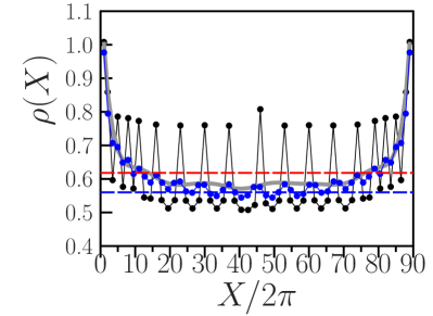
Figure 1: Local ion density distribution is shown along the ion chain for the sliding phase at $K=0.001$ (blue points connected by lines) and for the pinned phase at $K=0.01$ (black points connected by lines; the gray curve shows the smoothed distribution). Here the local density is defined as $\rho(X)=2\pi/(x_{i+1}-x_{i})$ and $X=(x_{i+1}+x_{i})/2$. The red dashed line corresponds to the fraction of golden mean density $\rho(X)=\nu_{g}-1=(\sqrt{5}-1)/2=0.618...$, and the blue dashed line corresponds to $\rho(X)=\nu=0.56$ obtained from the formfactor data (see Fig. 6 below). Here the ratio of $N$ and $L$ is $N/L=55/89\approx\nu_{g}\approx 0.618...\;$.

We note that in this work we consider only the problem of classical charges. Indeed, as shown in fki2007 the dimensionless Planck constant of the system is $\hbar_{\rm eff}=$ $\hbar/$ $(e\sqrt{m\ell/2\pi})$. For a typical lattice period $\ell\approx 1\rm\mu m$, $\nu\sim 1$ and ${{}^{40}}\rm Ca^{+}$ we have $\hbar_{\rm eff}\approx 10^{-5}$. For electrons on a periodic potential of liquid helium with the same period $\ell\approx 1\rm\mu m$ we have $\hbar_{\rm eff}\approx 2\times 10^{-3}$. Due to this reason we consider below only the classical dynamics of charges.

Following ztzs we model the dynamics of ions in the frame of Langevin approach (see e.g. politi ) with the equation of motion being

$$\dot{P}_{i}=\dot{v}_{i}=-\partial H/\partial x_{i}+E_{dc}-\eta P_{i}+g\xi_{i}(t)\;,\;\;\dot{x_{i}}=P_{i}=v_{i}\;.$$ (2)

The parameter $\eta$ describes phenomenologically the dissipative relaxation processes, and the amplitude of Langevin force $g$ is given by the fluctuation-dissipation theorem $g=\sqrt{2\eta T}$. We also use particle velocities $v_{i}=P_{i}$ (since mass is unity). The normally distributed random variables $\xi_{i}$ are defined by correlators $\langle\langle\xi_{i}(t)\rangle\rangle=0$, $\langle\langle\xi_{i}(t)\xi_{j}(t^{\prime})\rangle\rangle=\delta_{ij}\delta(t-t^{\prime})$. The amplitude of the static force is given by $E_{dc}$. The equations (2) are solved numerically by the 4th order Runge-Kutta integration with a time step $\Delta t$, at each such a step the Langevin contribution is taken into account, As in ztzs we usually use $\Delta t=0.02$ and $\eta=0.02$ with the results being not sensitive to these parameters.

The length of the system in 1D case is taken to be $2\pi L$ in $x$-direction with $L$ being the integer number of periods with periodic or hard-wall boundary conditions for $N$ ions inside the system. The dimensionless charge density is $\nu=N/L$ being related to the widing number of the KAM curves in the related symplectic map description of equilibrium positions of ions.

3 Density dependence of the Aubry transition

The equilibrium static positions of ions in a periodic potential are determined by the conditions $\partial H/\partial x_{i}=0$, $P_{i}=0$ aubry ; fki2007 . In the approximation of nearest neighbor interacting ions, this leads to the symplectic map for recurrent ion positions $x_{i}$

$$p_{i+1}=p_{i}+Kg(x_{i})\;,\;\;x_{i+1}=x_{i}+1/\sqrt{p_{i+1}}\;,$$ (3)

where the effective momentum conjugated to $x_{i}$ is $p_{i}=1/(x_{i}-x_{i-1})^{2}$ and the kick function $Kg(x_{i})=\left.-dV/dx\right|_{x=x_{i}}$ $=-K\sin x_{i}$.

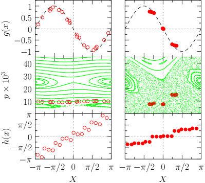
Figure 2: Functions related to the dynamical map obtained from the ground state equilibrium positions $x_{i}$ of ions at $K=0.001$ (open circles, left column) and $K=0.01$ (full circles, right column). Panels show: the kick function $g(x)$ (top); the phase space $(p,x)$ of the map with $g(x)=-K\sin x$ (green/light-gray points) and actual ion positions (red/gray circles) (middle); the hull function $h(x)$ (bottom). The ion positions are shown via the hull function $h(x)=(x_{i}+\pi)[{\rm mod}\;2\pi]-\pi$ versus $x=(2\pi(i-1)/\nu-\pi/2)[{\rm mod}\;2\pi]-\pi$, for the central $1/3$ part of the chain; $i\in(N/3,\ldots,2N/3)$. Here $N/L=60/89$.

As in fki2007 the validity of the map description is checked numerically finding the ground state configuration using numerical methods of energy minimization described in fki2007 ; aubry . In these simulations the Coulomb interactions between all ions are considered. Also we use the hard-wall boundary conditions at the ends of ion chain assuming that in the experiments it can be created by specific laser frequency detuning from resonant transition between ion energy levels. Due to these boundary conditions the local ion density is inhomogeneous since an ion near boundary vicinity has more pressure from other ions in the chain (a similar inhomogeneous local density $\nu(x_{i})=2\pi/(x_{i+1}-x_{i})$ appears for ions inside a global oscillator potential of a trap as discussed in fki2007 ). To avoid the non-homogeneity density effect we select the central part of the chain with approximately $1/3$ of all ions where the density is approximately constant. The examples of ion density for KAM sliding and Aubry pinned phases are shown in Fig. 1. The data show that the distribution of ions is relative smooth in the sliding phase and is rather peaked in the pinned phase. The selected density is chosen to be close to the inverse of the golden mean value $\nu=\tilde{\nu}_{g}=\nu_{g}^{-1}=\nu_{g}-1=(\sqrt{5}-1)/2=0.618...$ which is often used for stability analysis of KAM curves in symplectic maps (see e.g. lichtenberg ; meiss ). With the choice $N/L=55/89$, typical for common Frenkel-Kontorova model as a rational approximant to the golden mean, we have actually $\nu=0.56$, and we need to adjust the number of ions $N$ in order to approach the required value $\tilde{\nu}_{g}=0.618...$.

We note that this problem of local density change disappears if one restricts himself by the account for the nearest neighbors interactions between ions: in this approach the ions density becomes practically constant along the whole chain. This approach is used below in our simulations of kinetic properties of the system.

The analysis of ground state stationary positions of ions in a periodic potential is shown in Fig. 2 for the KAM sliding phase ($K=0.001$) and the Aubry pinned phase ($K=0.01$) at $N/L=60/89$ ratio which gives approximately the golden mean fraction $\nu\approx\tilde{\nu}_{g}\approx 0.618$ in the middle part of the chain. Even if the Coulomb interactions between all ions are considered the kick function $g(x)$ is close to the theoretical one $g(x)=-\sin x$. This shows that the approximation of nearest neighbors used in the symplectic map (3) gives us a good approximation of the system. For $K=0.001$ the positions of ions follow the invariant KAM curve while for $K=0.01$ the ion positions form an invariant Cantor set (cantori) appearing on the place of destroyed KAM curve. The hull function is defined as $h(x)=(x_{i}+\pi)[{\rm mod}\;2\pi]-\pi$ with $x=(2\pi(i-1)/\nu-\pi/2)[{\rm mod}\;2\pi]-\pi$, where $i\in(N/3,\ldots,2N/3)$. Indeed, at $K\rightarrow 0$ we have $h(x)=x$ with a smooth deformation for small perturbations while in the pinned phase we obtain the devil’s staircase corresponding to the fractal cantori structure. The transition from the smooth hull function to the devil’s staircase is visible in the data of Fig. 2 even if there is a certain spreading of points especially in the KAM phase which we attribute to a rather small value of $K=0.001$. Thus the obtained data show that with $\nu\approx 0.618$ the Aubry transition takes place at a certain $K_{c}(\nu)$ inside the interval $0.001<K_{c}(\nu)<0.01$.

It is important to note that a similar approximate symplectic map description for static charge positions is working well not only in the case of periodic potential but also for wiggling channel structures analyzed in snake .

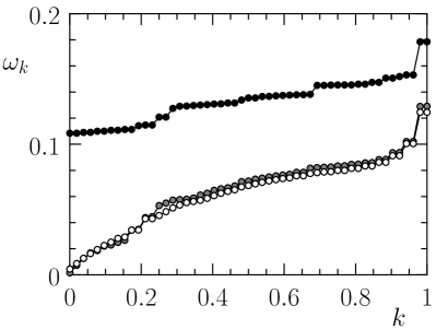
Figure 3: Spectrum of phonon excitations $\omega(k)$ as a function of scaled mode number $k=i/N$ ($i=1,\ldots,N-2$), for $K=0.001$ (bottom curve, open circles), $K=0.002$ (bottom curve, gray circles) and $K=0.015$ (top curve, full circles). Here there are $N=55$ ions and $L=89$ lattice periods.

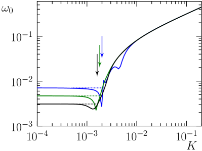
Figure 4: The lowest mode phonon frequency $\omega_{0}(K)$ vs the periodic potential coupling $K$. Blue, green and black curves correspond to $N/L=34/55,55/89$ and $89/144$. The position of the Aubry transition $K=K_{c}$ indicated by arrow is defined as an intersection of the curve $\omega_{0}(K)$ with the level shown by the dotted line at $\omega_{0}(K=0)$. Three arrows correspond to different winding numbers (densities) $\nu=34/55,55/89\text{ and }89/144$ and correspond to $K_{c}=0.002,0.0018\text{ and }0.0016$.

To obtain the critical amplitude in a more exact way we determine the static ion configuration at a fixed density $\nu=N/L$ and then compute the phonon spectrum $\omega(k)$ of small ion oscillations near the equilibrium positions. Such an approach was already used and described in aubry ; fki2007 . An example of the photon spectrum $\omega(k)$ is shown in Fig. 3 for $N/L=55/89$. Below the transition at $K<K_{c}(\nu)$ we have the linear acoustic type spectrum $\omega\approx C_{v}k$ of phonon type excitations describing ion oscillations near their static equilibrium positions like those shown in Fig. 2 at $N/L=60/89$. Here, $k=i/N$ plays the role of the wave vector and $C_{v}\approx 0.2$ is the sound velocity. The lowest phonon frequency goes to zero with the increase of the system size as $\omega(k=1/N)\approx C_{v}/N$. The spectrum becomes drastically different above the transition $K>K_{c}(\nu)$ with appearance of the optical gap $\omega_{0}$ in the spectrum $\omega(k)$. In fact, the gap $\omega_{0}$ is proportional to the Lyapunov exponent of symplectic map orbits located on the corresponding fractal cantori set aubry ; lichtenberg . It is independent of the system size $N$.

In principle, it is possible to search numerically for the value of $K_{c}(\nu)$ at which a nonzero optical gap appears in the spectrum $\omega(k)$. However, we find more useful to compute the dependence of lowest frequency $\omega_{0}=\omega(k=1/N)$ on the amplitude $K$. In the KAM phase we have $\omega_{0}(K)$ being independent of $K$ and thus we determine the critical $K_{c}(\nu)$ by the intersection of horizontal line $\omega_{0}(K)=\omega_{0}(K=0)$ with the curve of the spectrum $\omega_{0}(K)$ at higher $K$ values ($\omega_{0}(K=0)=\omega_{0}(K)$). The example of this intersection procedure is shown in Fig. 4 at increasing Fibonacci approximates $N/L=34/55,55/89,89/144$. We estimate the accuracy of this method of $K_{c}$ computation on the level of 10%-15% of $K_{c}$ value. At small sizes like $34/55$ a wiggling of curve at higher $K$ decreases the accuracy. But at longer sizes the result is stable. Thus we obtain the critical $K_{c}(\nu)\approx 0.0017$ for the irrational density $N/L=\nu=\nu_{g}=0.618...\;$, taking the average value for sizes $55/89$ and $89/144$.

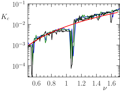
Figure 5: Dependence of the critical coupling $K_{c}$ on the winding number $\nu=N/L$. Blue, green and black curves correspond to $L=55,89$ and $144$; for each $L$ the number of ions $N$ takes all integer values up to corresponding highest/lowest $\nu$ value. The red curve corresponds to theoretical estimate: $K_{c}=0.034(\nu/1.618)^{3}$.

The numerically obtained dependence of the critical amplitude of Aubry transition $K_{c}(\nu)$ on ion density $\nu$ is shown in Fig. 5 for the range $0.5\leq\nu\leq 1.7$. The numerical values $K_{c}(\nu)$ are obtained as in Fig. 4 for the lattice size $L=55,89,144$ and for all integer $N$ values appearing inside the interval $0.5\leq\nu\leq 1.7$. On average the numerical values are in a good agreement with the theoretical expression given in fki2007

$$K_{c}(\nu)\approx 0.034(\nu/\nu_{g})^{3}\;,\;\;\nu_{g}=1.618...\;.$$ (4)

This formula is obtained on the basis of local reduction of map (3) to the Chirikov standard map with a homogeneous density of nonlinear resonances. For that the second equation (3) is linearized near $1/\sqrt{p}=2\pi/\nu_{g}$ that gives the Chirikov standard map with chaos parameter $K_{\rm eff}=K(2\pi/\nu_{g})^{3}/2$ and the critical value $K_{c}=0.034$ at $\nu_{g}=1.618...$ corresponding to $K_{\rm eff}\approx 1$. More details of this method are given in fki2007 ; chirikov ; lichtenberg ; scholarchi ). For $\nu=\nu_{g}=1.618...,$ the detailed numerical analysis gives $K_{c}(\nu)\approx 0.0462$ fki2007 ; ztzs (instead of $0.034$) and for $\nu=0.618...$ we have $K_{c}(\nu)\approx 0.0017$ (instead of $0.0189$). The strongest deviations from the theoretical dependence (4) take place at $\nu\approx 0.55$ and $\nu\approx 1.06$ with a significant drop of $K_{c}$. In fact, these $\nu$ values are located in the vicinity of main resonances with $\nu=1/2;1$ which are slightly shifted from their rational positions due to inhomogeneity of ion density appearing due to the hard-wall boundary conditions (see Fig. 1). In a vicinity of rational resonances there is a stochastic layer inside which the dynamical chaos emerges at rather small critical perturbations (see chirikov ; lichtenberg ).

In the following the analysis of the thermodynamic characteristics is done for $\nu\approx 0.618$. In the related Figs. 7-11 for rescaling of parameters to the dimensionless units we use $K_{c}=0.002$ which is close to the theoretical value $K=0.00189$ from (4).

Thus in global the numerical results obtained here for the dependence $K_{c}(\nu)$ on density are in good agreement with the theory (4) developed in fki2007 . The most striking feature of this dependence is the sharp decrease of $K_{c}$ with $\nu$. This allows to observe the Aubry transition at significantly smaller laser powers simply by a moderate decrease of density $\nu$ (see discussion below).

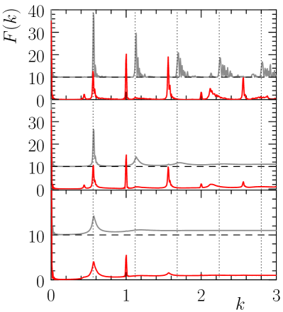
Figure 6: Dependence of the formfactor $F(k)$ on $k$ below the Aubry transition ($K=0.001<K_{c}=0.00189$) (KAM sliding phase, gray curves) and above ($K=0.01>K_{c}=0.002$) (pinned mode, red curves). For a clarity the gray curves are shifted up by 10. The temperature takes values $T=10^{-6},2\cdot 10^{-3},10^{-2}$ for top, middle and bottom panels respectively. Here $N/L=55/89$. Dotted curves indicate the peak positions at $k_{i}=\nu i$, where $\nu=0.56$ is the mean rotation number at the central region of the chain. (compare this value of $\nu$ to that in the Fig.1). The formfactor is calculated over central part of ion chain, contributions from 10 ions from each edge are ignored.

4 Formfactor of the ion structure

It is useful to characterize the structure of ions in a periodic potential by the formfactor $F(k)$ given by

$$F(k)=\left\langle\left|\sum_{i\neq j}^{N_{cr}}\exp\left(ik\left(x_{i}(t)-x_{j}(t)\right)\right)\right|^{2}\right\rangle/N_{cr}\;,$$ (5)

where the sum is taken by the central part of the chain with approximately $N_{cr}\approx N/3$. The positions of ions $x_{i}(t)$ at different moments of time are obtained at finite temperature $T$ with the Langevin equations (2) with averaging over time. Here we use the hard-wall boundary conditions and Coulomb interactions act between all electrons ions. Here we use the Metropolis algorithm for simulation of the thermal effects (see e.g. fki2007 ; snake ), rather than the Langevin equation, and the nearest neighbor approximation is not necessary.

The variation of $F(k)$ with temperature is shown in Fig. 6 for the KAM sliding phase and the Aubry pinned phase. In the KAM phase at $K<K_{c}$ the peaks of $F(k)$ are located at $k\approx i\nu$ corresponding to integer harmonics $i$ of average ion density $\nu\approx 0.56$ in the central part of the chain. In contrast, in the Aubry phase at $K>K_{c}$ there appear additional integer peaks at $k\approx i$ being commensurable with the lattice period. At low temperature $T=10^{-6}$ the peaks of $F(k)$ are well visible and clearly demonstrate the transition from incommensurate phase at $K<K_{c}$ to the quasi-commensurate phase above the Aubry transition at $K>K_{c}$. with the increase of temperature the high harmonics in $F(k)$ are washed out by thermal fluctuations. We think that the analysis of formafactor structure can be rather useful for experimental investigations of Aubry transition.

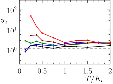
Figure 7: Dependence of Seebeck coefficient $S$ on temperature $T$ at different values $K/K_{c}=0$ (black), $1$ (blue), $2$ (green), $3$ (brown), $4$ (red). Here the ratio of number of $N$ ions to number of lattice periods $L$ is $N/L=21/34$ and $K_{c}=2\times 10^{-3}$. Dashed line shows $S=1.2$ value at $K=0$ for noninteracting particles.

5 Seebeck coefficient

The computations of the Seebeck coefficient $S$ are done in the frame of Langevin equations (2) with the hard-wall boundary conditions. We note that in the Aubry pinned phase long computational times are required. Thus we made simulations with times up to $t=10^{8}$. In these simulations for each ion we take into account the Coulomb interactions only with nearest left and right neighbor ions that allow to accelerate the computations. As in ztzs we ensured that the obtained results are not sensitive to inclusion of interactions with other neighbors.

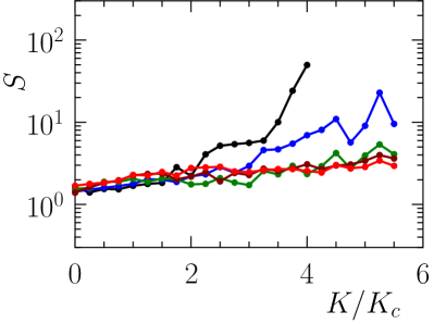
Figure 8: Seebeck dependence on $K$ at different temperatures $T/K_{c}=0.25$ (black), $0.5$ (blue), $1$ (green), $1.5$ (cyan), $2$ (red). Here the ratio of number of $N$ ions to number of lattice periods $L$ is $N/L=21/34$ and $K_{c}=2\times 10^{-3}$.

The computations of $S$ are done with the procedure developed in ztzs . At fixed temperature $T$ we apply a static field $E_{dc}$ which creates a voltage drop $\Delta V=E_{dc}2\pi L$ and a gradient of ion density $\nu(x)$ along the chain. Then at $E_{dc}=0$ within the Langevin equations (2) we impose a linear gradient of temperature $\Delta T$ along the chain and in the stabilized steady-state regime determine the charge density gradient of $\nu(x)$ along the chain (see e.g. Fig.2 in ztzs ). The data are obtained in the linear regime of relatively small $E_{dc}$ and $\Delta T$ values. Then the Seebeck coefficient is computed as $S=\Delta V/\Delta T$ where $\Delta V$ and $\Delta T$ are taken at such values that the density gradient from $\Delta V$ compensates the one from $\Delta T$.

The dependencies of $S$ on temperature $T$ at different amplitudes $K$ of the periodic potential are shown in Fig. 7. In the KAM sliding phase with $K\leq K_{c}$ there is no significant change of $S\approx 2$, which remains close to its value $S=1.2$ for free noninteracting particles. In contrast in the Aubry pinned phase with $K/K_{c}>1$ we obtain an exponential increase of $S$ at $T/K_{c}<0.5$. This increase of $S$ is especially visible for $K/K_{c}=4$ where the maximal reached value is $S\approx 50$.

We note that a similar strong growth of $S$ at low temperatures has been reported in experiments with quasi-one-dimensional conductor $\rm(TMTSF)_{2}PF_{6}$ espci where as high as $S=400$ value had been reached at low temperatures (see Fig. 3 in espci ).

The dependence of $S$ on $K$ is shown in Fig. 8. At low temperatures $T<K_{c}$ there is a sharp increase of $S$ with increase of $K>K_{c}$ with a maximal reached value $S\approx 60$. In a certain sense the increase of $K$ drives the system deeper and deeper into the insulating phase with larger and larger resistivity. Thus we can say that $S$ increases with the increase of sample resistivity. A similar dependence has been observed in experiments with two-dimensional electron gas in highly resistive (pinned) samples of micron size (see Fig. 8 in pepper ).

Thus we can say that our numerical results are in a qualitative agreement with the experiments espci ; pepper .

6 Figure of merit $ZT$

To determine the figure of merit $ZT$ we need to compute in addition to $S$ the electrical conductivity $\sigma$ and the heat conductivity $\kappa$. The computation of $\sigma$ is done by applying a weak $E_{dc}$ field acting on a circle with periodic boundary conditions. Then we compute the ion velocity $v_{ion}$ averaged over all particles and time interval. Then the charge current is $j=\nu v_{ion}/2\pi$ and $\sigma=j/E_{dc}$. At $K=0$ the ion crystal moves as a whole with $v_{ion}=E_{dc}/\eta$ corresponding to the conductivity of free particles $\sigma=\sigma_{0}=\nu/(2\pi\eta)$ that is confirmed by numerical simulations (see Fig. 9).

The dependence of $\sigma$ on $K$ and temperature $T$ is shown in Fig. 9. In the KAM sliding phase at $K<K_{c}$, $\sigma/\sigma_{0}$ is practically independent of $T$ and $K$. However, in the Aubry pinned phase at $K>K_{c}$ there is an exponential drop of $\sigma/\sigma_{0}$ with increase of $K$ and with decrease of $T$.

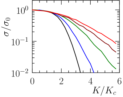
Figure 9: Dependence of conductivity on $K$ at different temperatures $T/K_{c}=0.25$ (black), $0.5$ (blue), $1$ (green), $1.5$ (brown), $2$ (red). Here the ratio of number of $N$ ions to number of lattice periods $L$ is $N/L=21/34$, $\eta=0.02$, $\sigma_{0}=\nu/(2\pi\eta)$ with $\nu=0.618$ and $K_{c}=2\times 10^{-3}$.

For the computation of heat conductivity $\kappa$ we use the approach developed in ztzs . The heat flow $J$ is related to the temperature gradient by the Fourier law with the thermal conductivity $\kappa$: $J=\kappa\partial T/\partial x$ thermobook ; politi . The heat flow is computed from forces acting on a given ion $i$ from left and right sides being respectively $f_{i}^{L}=\sum_{j<i}1/|x_{i}-x_{j}|^{2}$, $f_{i}^{R}=-\sum_{j>i}1/|x_{i}-x_{j}|^{2}$. For an ion moving with a velocity $v_{i}$ these forces create left and right energy flows $J_{L,R}=\langle f_{i}^{L,R}v_{i}\rangle_{t}\;$. In a steady state the mean ion energy is independent of time and $J_{L}+J_{R}=0$. But the difference of these flows gives the heat flow along the chain: $J=(J_{R}-J_{L})/2=\langle(f_{i}^{R}-f_{i}^{L})v_{i}/2\rangle_{t}\;$. We perform such computations of the heat flow, with hard wall boundary conditions. In addition to the method used in ztzs we perform time averaging using accurate numerical integration along the ions trajectories that cancels contribution of large oscillations due to periodical motion of ions. In this way we determine the thermal conductivity via the relation $\kappa=JL/\Delta T$. The obtained results for $\kappa$ are independent of small $\Delta T$. Our previous result confirm that the thermodynamic characteristic are independent of system size ztzs .

The dependence of heat conductivity $\kappa$ on $K$ and $T$ is shown in Fig. 10. For convenience we present the ratio of $\kappa$ to $\kappa_{0}=\sigma_{0}K_{c}$ to have the results in dimensionless units. There is an exponential decrease of $\kappa/\kappa_{0}$ with increase of $K>K_{c}$ showing that for ionic phonons the propagation along the chain becomes more difficult at high $K$ amplitudes. The decrease of $T$ leads to a decrease of $\kappa/\kappa_{0}$ but this drop is less pronounced comparing to those for $\sigma/\sigma_{0}$.

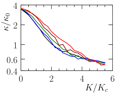
Figure 10: Dependence of heat conductivity $\kappa$ on $K$ at different temperatures $T/K_{c}=0.25$ (black), $0.5$ (blue), $1$ (green), $1.5$ (brown), $2$ (red). Here the ratio of number of $N$ ions to number of lattice periods $L$ is $N/L=21/34$, $\eta=0.02$, $\kappa_{0}=\sigma_{0}K_{c}$ and $K_{c}=2\times 10^{-3}$.

From the obtained values of $S$, $\sigma$ and $\kappa$ at $\nu\approx 0.618$ we compute the figure of merit $ZT$ shown in Fig. 11 as a function of $K/K_{c}$ at different temperatures. At fixed $T$ there is an optimal maximal $ZT$ value located approximately at $K/K_{c}\approx 2.5$ while at smaller and higher $K/K_{c}$ values we have a decrease of $ZT$. The maximal $ZT$ value increases with the growth of temperature and the width of the peak becomes broader. At the maximum with $T/K_{c}=2$ and $K/K_{c}=2.5$ we obtain $ZT\approx 8$. This maximal $ZT$ value is by factor $2$ larger than the value obtained at $\nu\approx 1.618$, $T/K_{c}\approx 3$ and $K/K_{c}\approx 3.5$ in ztzs . We suppose that a more dilute ion density favors more efficient thermodynamical characteristics.

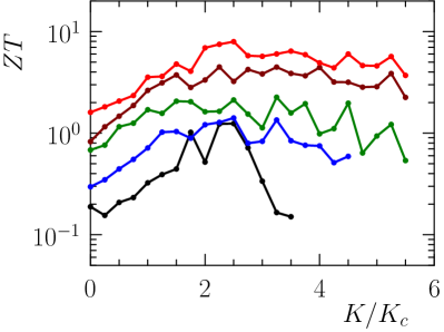
Figure 11: Dependence of figure of merit $ZT$ on $K$ at different temperatures $T/K_{c}=0.25$ (black), $0.5$ (blue), $1$ (green), $1.5$ (brown), $2$ (red). Here the ratio of number of $N$ ions to number of lattice periods $L$ is $N/L=21/34$, $\eta=0.02$ and $K_{c}=2\times 10^{-3}$.

Our studies are done for the strictly 1D case. It is important to consider extensions to the two-dimensional (2D) case which may be useful for electrons on liquid helium and material science. Indeed, in quasi-1D case it is known that transfer dynamics can lead to excitation of transfer modes and zigzag instabilities morigi ; peeters . However, the recent results reported for 2D Wigner crystal transport indicate that there is similarity between 1D and 2D properties and thus we expect that the obtained results will be useful for higher-dimensional systems.

7 Discussion

In this work we analyzed the properties of cold ion chain placed in a periodic potential. The results show the emergence of Aubry transition from KAM sliding phase to Aubry pinned phase when the amplitude of the potential exceeds a critical value $V_{A}=K_{c}(\nu)e^{2}/(\ell/2\pi)$. For a typical period of optical lattice $\ell=1\rm\mu m$ and dimensionless ion density per period $\nu=1.618$ this corresponds to $V_{A}\approx 3\rm K$ (Kelvin) that would require rather strong laser power for creation of such optical potential. However, with a decrease of $\nu$ we have a cubic drop of $V_{A}$ and thus for $\nu=0.38$ we need only $V_{A}\approx 0.04\rm K$ that is much more accessible for optical lattice experiments.

The interest of the Aubry phase is related to high thermodynamic properties appearing in this phase. Thus we show that one can reach in this phase the high values of Seebeck coefficient $S\approx 50k_{B}/e\approx 4400\rm\mu V/K$ which approaches to the record experimental values $S\approx 400k_{B}/e$ observed in quasi-one-dimensional materials espci and with two-dimensional electron gas in small disordered samples with $S\sim 50k_{B}/e$ pepper . Even more remarkable is that in this phase the figure of merit can be as such high as $ZT\approx 8$ being above the record experimental values ztsci2017 . We suppose that for cold ions in optical lattices the voltage difference $\Delta V$ can be easily created by a weak external static electric field while the temperature difference $\Delta T$ at the ends of the lattice can be generated by additional laser heating. Thus such experiments would allow to investigate the thermodynamical properties of Wigner crystal of cold ions in optical lattice. We assume that the investigations of thermoelectric properties with cold ions in optical lattices may bring us to a deep understanding of thermoelectricity which will be further used for selection of optimal thermoelectric materials.

Also we think that the simple models considered here rise an important challenge for computational methods of quantum chemistry where interactions of electrons and atoms are taking into account in the computations of band structures but after that the thermoelectric characteristics are computed for effectively noninteracting electrons (see e.g. kozinsky ; melendez ). We argue that our results clearly show that the high thermoelectric characteristics appear only in the Aubry pinned phase where the interactions between charges play a crucial role. We argue that our results challenge the further development of methods of quantum chemistry.

Thus the above analysis clearly demonstrates the importance of Aubry pinned phase for high thermoelectric performance. Due to that the experimental investigations of the Aubry transition with cold ions in optical lattices and electrons on liquid helium will bring to us important fundamental results useful for development of efficient thermoelectric materials.

8 Acknowledgments

This work was supported in part by the Pogramme Investissements d’Avenir ANR-11-IDEX-0002-02, reference ANR-10-LABX-0037-NEXT (project THETRACOM); it was granted access to the HPC resources of CALMIP (Toulouse) under the allocation 2017-P0110. This work was also supported in part by the Programme Investissements d’Avenir ANR-15-IDEX-0003, ISITE-BFC (project GNETWORKS). For OVZ this work is partially supported by the Ministry of Education and Science of the Russian Federation. One of us (DLS) thanks R.V.Belosludov and V.R.Belosludov for discussions of methods of quantum chemistry used for computations of thermoelectric characteristics in real materials.

References

- (1) E. Wigner, On the interaction of electrons in metals, Phys. Rev. 46, 1002 (1934).
- (2) G. Birkl, S. Kassner, and H. Walther, Multiple-shell structures of laser-cooled ions in a quandrupole storage ring, Nature 357, 310 (1992).
- (3) D.H.E.Dubin and T.M. O’Neil, Trapped nonneutral plasmas, liquids, and crystals (the thermal equilibrium states), Rev. Mod. Phys. 71, 87 (1999).
- (4) Y. Monarkha and K. Kono, Two-Ddmensional Coulomb liquids and solids, Springer-Verlag, Berlin (2004).
- (5) J.S. Meyer and K.A. Matveev, Wigner crystal physics in quantum wires, J. Phys. C.: Condens. Mat. 21, 023203 (2009).
- (6) V.E. Fortov, A.V. Ivlev, S.A. Khrapak, A.G. Khrapak, and G.E. Morfill, Complex (dusty) plasmas: current status, open issues, perspectives, Phys. Rep. 421, 1 (2005)
- (7) J.I. Cirac and P. Zoller, Quantum computations with cold trapped ions, Phys. Rev. Lett. 74, 4091 (1995).
- (8) R. Blatt and D. Wineland, Entangled states of trapped atomic ions, Nature 453, 1008 (2008).
- (9) M. Johanning, A.F. Varon and C. Wunderlich, Quantum simulations with cold trapped ions, J, Phys. B: At. Mol. Opt. Phys. 42, 154009 (2009).
- (10) R. Blatt and C.F. Roos, Quantum simulations with trapped ions, Nature Phys. 8, 277 (2012).
- (11) G. Pagano, P.W. Hess, H.B. Kaplan, W.L. Tan, P. Richerme, P. Becker, A. Kyprianidis, J. Zhang, E. Birckelbaw, M.R. Hernandez, Y. Wu and C. Monroe, Cryogenic trapped-ion system for large scale quantum simulation, arXiv:1802.03118 [quant-ph] (2018).
- (12) I. Garcia-Mata, O.V. Zhirov, and D.L. Shepelyansky, Frenkel-Kontorova model with cold trapped ions, Eur. Phys. J. D 41, 325 (2007).
- (13) S. Aubry, The twist map, the extended Frenkel-Kontorova model and the devil’s staircase, Physica D 7 (1983) 240.
- (14) O.M. Braun and Yu.S. Kivshar, The Frenkel-Kontorova Model: Concepts, Methods, Applications, Springer-Verlag, Berlin (2004).
- (15) B. V. Chirikov, A universal instability of many-dimensional oscillator systems , Phys. Rep. 52 (1979) 263.
- (16) A.J.Lichtenberg, M.A.Lieberman, Regular and chaotic dynamics, Springer, Berlin (1992).
- (17) J.D. Meiss, Symplectic maps, variational principles, and transport, Rev. Mod. Phys. 64(3), 795 (1992).
- (18) B. Chirikov and D. Shepelyansky, Chirikov standard map, Scholarpedia 3(3), 3550 (2008).
- (19) T. Pruttivarasin, M. Ramm, I. Talukdar, A. Kreuter, and H. Haffner, Trapped ions in optical lattices for probing oscillator chain models, New J. Phys. 13, 075012 (2011).
- (20) A. Bylinskii, D. Gangloff, and V. Vuletic, Tuning friction atom-by-atom in an ion-crystal simulator, Science 348, 1115 (2015).
- (21) A. Bylinskii, D. Gangloff, I. Countis, and V. Vuletic, Observation of Aubry-type transition in finite atom chains via friction, Nature Mat. 11, 717 (2016).
- (22) J.Kiethe, R. Nigmatullin, D. Kalincev, T. Schmirander, and T.E. Mehlstaubler, Probing nanofriction and Aubry-type signatures in a finite self-organized system, Nature Comm. 8 15364 (2017).
- (23) A. Benassi, A. Vanossi, and E. Tosatti, Nanofriction in cold ion traps, Nature Comm. 2, 236 (2011).
- (24) D. Mandelli and E. Tosatti, Microscopic friction emulators, Nature 526, 332 (2015).
- (25) N. Manini, G. Mistura, G. Paolicelli, E. Tosatti, and A. Vanossi, Current trends in the physics of nanoscale friction, Adv. Phys. X 2(3), 569 (2017).
- (26) M.Y. Zakharov, D. Demidov and D.L. Shepelyansky, Wigner crystal diode, arXiv:1901.05231 [cond-mat.mes-hall] (2019).
- (27) O.V. Zhirov, and D.L. Shepelyansky, Thermoelectricity of Wigner crystal in a periodic potential, Europhys. Lett. 103, 68008 (2013).
- (28) A.F. Ioffe, Semiconductor thermoelements, and thermoelectric cooling, Infosearch, Ltd (1957).
- (29) A.F. Ioffe and L.S. Stil’bans, Physical problems of thermoelectricity, Rep. Prog. Phys. 22, 167 (1959).
- (30) A. Majumdar, Thermoelectricity in semiconductor nanostructures, Science 303, 777 (2004).
- (31) H.J. Goldsmid, Introduction to thermoelectricity, Springer, Berlin (2009).
- (32) N. Li, J. Ren, L. Wang, G. Zhang, P. Hanggi, and B. Li, Phononics: manipulating heat flow with electronic analogs and beyond, Rev. Mod. Phys. 84, 1045 (2012).
- (33) B.G. Levi, Simple compound manifests record-high thermoelectric performance, Phys. Tod. 67(6), 14 (2014).
- (34) J. He, and T.M. Tritt, Advances in thermoelectric materials research: looking back and moving forward, Science 357, eaak9997 (2017).
- (35) J.P. Heremans, M.S. Dresselhaus, L.E. Bell and D.T. Morelli, When thermoelectrics reached the nanoscale, Nature Nanotech. 8, 471 (2013).
- (36) S. Bang, D. Wee, A. Li, M. Fornari and B. Kozinsky, Thermoelectric properties of pnictogen-substituted skutterudites with alkaline-earth fillers using first-principles calculations, J. Appl. Phys. 119, 205102 (2016).
- (37) R.L. Gonzalez-Romeo, A. Antonelli and J.J. Melendez, Insights into the thermoelectric properties of SnSe from ab initio calculations, Phys. Chem. Chem. Phys. 19, 12804 (2017).
- (38) D.G.-Rees, S.-S. Yeh, B.-C. Lee, K. Kono, and J.-J.Lin, Bistable transport properties of a quasi-one-dimensional Wigner solid on liquid helium under continuous driving, Phys. Rev. B 96, 205438 (2017).
- (39) J.-Y. Lin, A.V. Smorodin, A.O. Badrutdinov, and D. Konstantinov, Transport properties of a quasi-1D Wigner solid on liquid helium confined in a microchannel with periodic potential, J. Low Temp. Phys. doi.org/10.1007/s10909-018-2089-7 (2018).
- (40) T. Brazda, A. Silva, N. Manini, A. Vanossi, R. Guerra, E. Tosatti, and C. Bechinger, Experimental observation of the Aubry transition in two-dimensional colloidal monolayers, Phys. Rev. X 8, 011050 (2018).
- (41) S. Lepri, R. Livi, and A. Politi, Thermal conduction in classical low-dimensional lattices, Phys. Rep. 377, 1 (2003).
- (42) O.V. Zhirov, and D.L. Shepelyansky, Wigner crystal in snaked nanochannels, Eur. Phys. J. B 82, 63 (2011).
- (43) D. Shepelyansky, Chirikov criterion, Scholarpedia 4(9), 8567 (2009).
- (44) Y. Machida, X. Lin, W. Kang, K. Izawa and K. Behnia, Colossal Seebeck Coefficient of Hopping Electrons in , Phys. Rev. Lett. 116, 087003 (2016).
- (45) V. Narayan, M. Pepper, J. Griffiths, H. Beere, F. Sfigakis, G. Jones, D. Ritchie and A. Ghosh, Unconventional metallicity and giant thermopower in a strongly interacting two-dimensional electron system, Phys. Rev. B 86, 125406 (2012).
- (46) E. Shimshoni, G. Morigi, and S. Fishman, Quantum zigzag transition in ion chains, Phys. Rev. Lett. 106, 010401 (2011).
- (47) J.C.N. Carvalho, W.P. Ferreira, G.A. Farias and F.M. Peeters, Yukava particles confined in a channel and subject to a periodic potential: ground state and normal modes, Phys. Rev. B 83, 094109 (2011).