Learning Mean-Field Games

Abstract

This paper presents a general mean-field game (GMFG) framework for simultaneous learning and decision-making in stochastic games with a large population. It first establishes the existence of a unique Nash Equilibrium to this GMFG, and explains that naively combining Q-learning with the fixed-point approach in classical MFGs yields unstable algorithms. It then proposes a Q-learning algorithm with Boltzmann policy (GMF-Q), with analysis of convergence property and computational complexity. The experiments on repeated Ad auction problems demonstrate that this GMF-Q algorithm is efficient and robust in terms of convergence and learning accuracy. Moreover, its performance is superior in convergence, stability, and learning ability, when compared with existing algorithms for multi-agent reinforcement learning.

1 Introduction

Motivating example.

This paper is motivated by the following Ad auction problem for an advertiser. An Ad auction is a stochastic game on an Ad exchange platform among a large number of players, the advertisers. In between the time a web user requests a page and the time the page is displayed, usually within a millisecond, a Vickrey-type of second-best-price auction is run to incentivize interested advertisers to bid for an Ad slot to display advertisement. Each advertiser has limited information before each bid: first, her own valuation for a slot depends on an unknown conversion of clicks for the item; secondly, she, should she win the bid, only knows the reward after the user’s activities on the website are finished. In addition, she has a budget constraint in this repeated auction.

The question is, how should she bid in this online sequential repeated game when there is a large population of bidders competing on the Ad platform, with unknown distributions of the conversion of clicks and rewards?

Besides the Ad auction, there are many real-world problems involving a large number of players and unknown systems. Examples include massive multi-player online role-playing games MMORPG , high frequency tradings algo_trade_mfg , and the sharing economy sharing_eco .

Our work.

Motivated by these problems, we consider a general framework of simultaneous learning and decision-making in stochastic games with a large population. We formulate a general mean-field-game (GMFG) with incorporation of action distributions, (randomized) relaxed policies, and with unknown rewards and dynamics. This general framework can also be viewed as a generalized version of MFGs of McKean-Vlasov type MKV , which is a different paradigm from the classical MFG. It is also beyond the scope of the existing Q-learning framework for Markov decision problem (MDP) with unknown distributions, as MDP is technically equivalent to a single player stochastic game.

On the theory front, this general framework differs from all existing MFGs. We establish under appropriate technical conditions, the existence and uniqueness of the Nash equilibrium (NE) to this GMFG. On the computational front, we show that naively combining Q-learning with the three-step fixed-point approach in classical MFGs yields unstable algorithms. We then propose a Q-learning algorithm with Boltzmann policy (GMF-Q), establish its convergence property and analyze its computational complexity. Finally, we apply this GMF-Q algorithm to the Ad auction problem, where this GMF-Q algorithm demonstrates its efficiency and robustness in terms of convergence and learning. Moreover, its performance is superior, when compared with existing algorithms for multi-agent reinforcement learning for convergence, stability, and learning accuracy.

Related works.

On learning large population games with mean-field approximations, YYTXZ2017 focuses on inverse reinforcement learning for MFGs without decision making, YLLZZW2018 studies an MARL problem with a first-order mean-field approximation term modeling the interaction between one player and all the other finite players, and KC2013 and YMMS2014 consider model-based adaptive learning for MFGs in specific models (e.g., linear-quadratic and oscillator games). More recently, Manymany studies the local convergence of actor-critic algorithms on finite time horizon MFGs, and rl_mfg_local proposes a policy-gradient based algorithm and analyzes the so-called local NE for reinforcement learning in infinite time horizon MFGs. For learning large population games without mean-field approximation, see MARL_literature2 ; MARL_literature1 and the references therein. In the specific topic of learning auctions with a large number of advertisers, CRZMWYG2017 and JSLGWZ2018 explore reinforcement learning techniques to search for social optimal solutions with real-word data, and IJS2011 uses MFGs to model the auction system with unknown conversion of clicks within a Bayesian framework.

However, none of these works consider the problem of simultaneous learning and decision-making in a general MFG framework. Neither do they establish the existence and uniqueness of the (global) NE, nor do they present model-free learning algorithms with complexity analysis and convergence to the NE. Note that in principle, global results are harder to obtain compared to local results.

2 Framework of General MFG (GMFG)

2.1 Background: classical $N$-player Markovian game and MFG

Let us first recall the classical $N$-player game. There are $N$ players in a game. At each step $t$, the state of player $i\ \ (=1,2,\cdots,N)$ is $s^{i}_{t}\in\mathcal{S}\subseteq\mathbb{R}^{d}$ and she takes an action $a^{i}_{t}\in\mathcal{A}\subseteq\mathbb{R}^{p}$. Here $d,p$ are positive integers, and $\mathcal{S}$ and $\mathcal{A}$ are compact (for example, finite) state space and action space, respectively. Given the current state profile of $N$-players ${\bf s}_{t}=(s^{1}_{t},\dots,s^{N}_{t})\in\mathcal{S}^{N}$ and the action $a^{i}_{t}$, player $i$ will receive a reward $r^{i}({\bf s}_{t},a^{i}_{t})$ and her state will change to $s^{i}_{t+1}$ according to a transition probability function $P^{i}({\bf s}_{t},a^{i}_{t})$.

A Markovian game further restricts the admissible policy/control for player $i$ to be of the form $a^{i}_{t}=\pi^{i}_{t}({\bf s}_{t})$. That is, $\pi^{i}_{t}:\mathcal{S}^{N}\rightarrow\mathcal{P}(\mathcal{A})$ maps each state profile ${\bf s}\in\mathcal{S}^{N}$ to a randomized action, with $\mathcal{P}(\mathcal{X})$ the space of probability measures on space $\mathcal{X}$. The accumulated reward (a.k.a. the value function) for player $i$, given the initial state profile ${\bf s}$ and the policy profile sequence $\boldsymbol{\pi}:=\{\boldsymbol{\pi}_{t}\}_{t=0}^{\infty}$ with $\boldsymbol{\pi}_{t}=(\pi^{1}_{t},\dots,\pi^{N}_{t})$, is then defined as

$$V^{i}({\bf s},\boldsymbol{\pi}):=\mathbb{E}\left[\sum_{t=0}^{\infty}\gamma^{t}r^{i}({\bf s}_{t},a^{i}_{t})\Big{|}{\bf s}_{0}={\bf s}\right],$$ (1)

where $\gamma\in(0,1)$ is the discount factor, $a^{i}_{t}\sim\pi^{i}_{t}({\bf s}^{t})$, and $s^{i}_{t+1}\sim P^{i}({\bf s}_{t},a_{t}^{i})$. The goal of each player is to maximize her value function over all admissible policy sequences.

In general, this type of stochastic $N$-player game is notoriously hard to analyze, especially when $N$ is large PR05 . Mean field game (MFG), pioneered by HMC2006 and LL2007 in the continuous settings and later developed in MFG_n_conv ; MFG_gomes ; MFG_binact ; MFG_discrete_time ; MFG_discrete_time2 for discrete settings, provides an ingenious and tractable aggregation approach to approximate the otherwise challenging $N$-player stochastic games. The basic idea for an MFG goes as follows. Assume all players are identical, indistinguishable and interchangeable, when $N\to\infty$, one can view the limit of other players’ states ${\bf s}_{t}^{-i}=(s_{t}^{1},\dots,s_{t}^{i-1},s_{t}^{i+1},\dots,s_{t}^{N})$ as a population state distribution $\mu_{t}$ with $\mu_{t}(s):=\lim_{N\rightarrow\infty}\frac{\sum_{j=1,j\neq i}^{N}\textbf{I}_{s_{t}^{j}=s}}{N}$. Due to the homogeneity of the players, one can then focus on a single (representative) player. That is, in an MFG, one may consider instead the following optimization problem,

$$\begin{array}[]{ll}\text{maximize}_{\boldsymbol{\pi}}&V(s,\boldsymbol{\pi},\boldsymbol{\mu}):=\mathbb{E}\left[\sum\limits_{t=0}^{\infty}\gamma^{t}r(s_{t},a_{t},\mu_{t})|s_{0}=s\right]\\ \text{subject to}&s_{t+1}\sim P(s_{t},a_{t},\mu_{t}),\quad a_{t}\sim\pi_{t}(s_{t},\mu_{t}),\end{array}$$

where $\boldsymbol{\pi}:={\{\pi_{t}\}_{t=0}^{\infty}}$ denotes the policy sequence and $\boldsymbol{\mu}:=\{\mu_{t}\}_{t=0}^{\infty}$ the distribution flow. In this MFG setting, at time $t$, after the representative player chooses her action $a_{t}$ according to some policy $\pi_{t}$, she will receive reward $r(s_{t},a_{t},\mu_{t})$ and her state will evolve under a controlled stochastic dynamics of a mean-field type $P(\cdot|s_{t},a_{t},\mu_{t})$. Here the policy $\pi_{t}$ depends on both the current state $s_{t}$ and the current population state distribution $\mu_{t}$ such that $\pi:\mathcal{S}\times\mathcal{P}(\mathcal{S})\rightarrow\mathcal{P}(\mathcal{A})$.

2.2 General MFG (GMFG)

In the classical MFG setting, the reward and the dynamic for each player are known. They depend only on $s_{t}$ the state of the player, $a_{t}$ the action of this particular player, and $\mu_{t}$ the population state distribution. In contrast, in the motivating auction example, the reward and the dynamic are unknown; they rely on the actions of all players, as well as on $s_{t}$ and $\mu_{t}$.

We therefore define the following general MFG (GMFG) framework. At time $t$, after the representative player chooses her action $a_{t}$ according to some policy $\pi:\mathcal{S}\times\mathcal{P}(\mathcal{S})\rightarrow\mathcal{P}(\mathcal{A})$, she will receive a reward $r(s_{t},a_{t},\mathcal{L}_{t})$ and her state will evolve according to $P(\cdot|s_{t},a_{t},\mathcal{L}_{t})$, where $r$ and $P$ are possibly unknown. The objective of the player is to solve the following control problem:

$$\begin{array}[]{ll}\text{maximize}_{\boldsymbol{\pi}}&V(s,\boldsymbol{\pi},\boldsymbol{\mathcal{L}}):=\mathbb{E}\left[\sum\limits_{t=0}^{\infty}\gamma^{t}r(s_{t},a_{t},{\color[rgb]{0,0,0}\mathcal{L}_{t}})|s_{0}=s\right]\\ \text{subject to}&s_{t+1}\sim P(s_{t},a_{t},{\color[rgb]{0,0,0}\mathcal{L}_{t}}),\quad a_{t}\sim\pi_{t}(s_{t},\mu_{t}).\end{array}$$ (GMFG)

Here, $\boldsymbol{\mathcal{L}}:=\{\mathcal{L}_{t}\}_{t=0}^{\infty}$, with $\mathcal{L}_{t}=\mathbb{P}_{s_{t},a_{t}}\in\mathcal{P}(\mathcal{S}\times\mathcal{A})$ the joint distribution of the state and the action (i.e., the population state-action pair). $\mathcal{L}_{t}$ has marginal distributions $\alpha_{t}$ for the population action and $\mu_{t}$ for the population state. Notice that $\{\mathcal{L}_{t}\}_{t=0}^{\infty}$ could depend on time. Namely, an infinite time horizon MFG could still have time-dependent NE solution due to the mean information process (game interaction) in the MFG. This is fundamentally different from the theory of single-agent MDP where the optimal control, if exists uniquely, would be time independent in an infinite time horizon setting.

In this framework, we adopt the well-known Nash Equilibrium (NE) for analyzing stochastic games.

Definition 2.1 (NE for GMFGs).

In (GMFG), a player-population profile $(\boldsymbol{\pi}^{\star},\boldsymbol{\mathcal{L}}^{\star}):=(\{\pi_{t}^{\star}\}_{t=0}^{\infty},\{\mathcal{L}_{t}^{\star}\}_{t=0}^{\infty})$ is called an NE if

1. (Single player side) Fix $\boldsymbol{\mathcal{L}}^{\star}$, for any policy sequence $\boldsymbol{\pi}:=\{\pi_{t}\}_{t=0}^{\infty}$ and initial state $s\in\mathcal{S}$,

   $$V\left(s,\boldsymbol{\pi}^{\star},\boldsymbol{\mathcal{L}}^{\star}\right)\geq V\left(s,\boldsymbol{\pi},\boldsymbol{\mathcal{L}}^{\star}\right).$$ (2)

2. (Population side) $\mathbb{P}_{s_{t},a_{t}}={\mathcal{L}_{t}^{\star}}$ for all $t\geq 0$, where $\{s_{t},a_{t}\}_{t=0}^{\infty}$ is the dynamics under the policy sequence $\boldsymbol{\pi}^{\star}$ starting from $s_{0}\sim\mu_{0}^{\star}$, with $a_{t}\sim\pi_{t}^{\star}(s_{t},{\color[rgb]{0,0,0}\mu_{t}^{\star}})$, $s_{t+1}\sim P(\cdot|s_{t},a_{t},{\color[rgb]{0,0,0}\mathcal{L}_{t}^{\star}})$, and $\mu_{t}^{\star}$ being the population state marginal of $\mathcal{L}_{t}^{\star}$.

The single player side condition captures the optimality of $\boldsymbol{\pi}^{\star}$, when the population side is fixed. The population side condition ensures the “consistency” of the solution: it guarantees that the state and action distribution flow of the single player does match the population state and action sequence $\boldsymbol{\mathcal{L}}^{\star}$.

2.3 Example: GMFG for the repeated auction

Now, consider the repeated Vickrey auction with a budget constraint in Section 1. Take a representative advertiser in the auction. Denote $s_{t}\in\{0,1,2,\cdots,s_{\max}\}$ as the budget of this player at time $t$, where $s_{\max}\in\mathbb{N}^{+}$ is the maximum budget allowed on the Ad exchange with a unit bidding price. Denote $a_{t}$ as the bid price submitted by this player and $\alpha_{t}$ as the bidding/(action) distribution of the population. The reward for this advertiser with bid $a_{t}$ and budget $s_{t}$ is

$$r_{t}={\color[rgb]{0,0,0}\textbf{I}_{w_{t}^{M}=1}}\left[(v_{t}-a^{M}_{t})-(1+\rho){\color[rgb]{0,0,0}\textbf{I}_{s_{t}<a^{M}_{t}}}(a^{M}_{t}-s_{t})\right].$$ (3)

Here $w^{M}_{t}$ takes values $1$ and $0$, with $w_{t}^{M}=1$ meaning this player winning the bid and $0$ otherwise. The probability of winning the bid would depend on $M$, the index for the game intensity, and $\alpha_{t}$. (See discussion on $M$ in Appendix H.1.) The conversion of clicks at time $t$ is $v_{t}$ and follows an unknown distribution. $a^{M}_{t}$ is the value of the second largest bid at time $t$, taking values from $0$ to $s_{\max}$, and depends on both $M$ and $\mathcal{L}_{t}$. Should the player win the bid, the reward $r_{t}$ consists of two parts, corresponding to the two terms in (3). The first term is the profit of wining the auction, as the winner only needs to pay for the second best bid $a_{t}^{M}$ in a Vickrey auction. The second term is the penalty of overshooting if the payment exceeds her budget, with a penalty rate $\rho$. At each time $t$, the budget dynamics $s_{t}$ follows,

$${s}_{t+1}=\left\{\begin{array}[]{ll}s_{t},&w^{M}_{t}\neq 1,\\ s_{t}-a^{M}_{t},&w^{M}_{t}=1\text{ and }a^{M}_{t}\leq s_{t},\\ 0,&w^{M}_{t}=1\text{ and }a^{M}_{t}>s_{t}.\end{array}\right.$$

That is, if this player does not win the bid, the budget will remain the same. If she wins and has enough money to pay, her budget will decrease from $s_{t}$ to $s_{t}-a^{M}_{t}$. However, if she wins but does not have enough money, her budget will be $0$ after the payment and there will be a penalty in the reward function. Note that in this game, both the rewards $r_{t}$ and the dynamics $s_{t}$ are unknown a priori.

In practice, one often modifies the dynamics of $s_{t+1}$ with a non-negative random budget fulfillment $\Delta({s}_{t+1})$ after the auction clearing GKP2012 , such that $\hat{s}_{t+1}={s}_{t+1}+\Delta({s}_{t+1})$. One may see some particular choices of $\Delta({s}_{t+1})$ in the experiment section (Section 5).

3 Solution for GMFGs

We now establish the existence and uniqueness of the NE to (GMFG), by generalizing the classical fixed-point approach for MFGs to this GMFG setting. (See HMC2006 and LL2007 for the classical case). It consists of three steps.

Step A.

Fix $\boldsymbol{\mathcal{L}}:=\{\mathcal{L}_{t}\}_{t=0}^{\infty}$, (GMFG) becomes the classical optimization problem. Indeed, with $\boldsymbol{\mathcal{L}}$ fixed, the population state distribution sequence $\boldsymbol{\mu}:=\{\mu_{t}\}_{t=0}^{\infty}$ is also fixed, hence the space of admissible policies is reduced to the single-player case. Solving (GMFG) is now reduced to finding a policy sequence $\pi_{t,\boldsymbol{\mathcal{L}}}^{\star}\in\Pi:=\{\pi\,|\,\pi:\mathcal{S}\rightarrow\mathcal{P}(\mathcal{A})\}$ over all admissible $\boldsymbol{\pi}_{\boldsymbol{\mathcal{L}}}=\{\pi_{t,\boldsymbol{\mathcal{L}}}\}_{t=0}^{\infty}$, to maximize

$$\begin{array}[]{ll}V(s,\boldsymbol{\pi}_{\boldsymbol{\mathcal{L}}},\boldsymbol{\mathcal{L}}):=&\mathbb{E}\left[\sum\limits_{t=0}^{\infty}\gamma^{t}r(s_{t},a_{t},\mathcal{L}_{t})|s_{0}=s\right],\\ \text{subject to}&s_{t+1}\sim P(s_{t},a_{t},\mathcal{L}_{t}),\quad a_{t}\sim\pi_{t,\boldsymbol{\mathcal{L}}}(s_{t}).\end{array}$$

Notice that with $\boldsymbol{\mathcal{L}}$ fixed, one can safely suppress the dependency on $\mu_{t}$ in the admissible policies. Moreover, given this fixed $\boldsymbol{\mathcal{L}}$ sequence and the solution $\boldsymbol{\pi}_{\boldsymbol{\mathcal{L}}}^{\star}:=\{\pi_{t,\boldsymbol{\mathcal{L}}}^{\star}\}_{t=0}^{\infty}$, one can define a mapping from the fixed population distribution sequence $\boldsymbol{\mathcal{L}}$ to an arbitrarily chosen optimal randomized policy sequence. That is,

$$\Gamma_{1}:\{\mathcal{P}(\mathcal{S}\times\mathcal{A})\}_{t=0}^{\infty}\rightarrow\{\Pi\}_{t=0}^{\infty},$$

such that $\boldsymbol{\pi}_{\boldsymbol{\mathcal{L}}}^{\star}=\Gamma_{1}(\boldsymbol{\mathcal{L}})$. Note that this $\boldsymbol{\pi}_{\boldsymbol{\mathcal{L}}}^{\star}$ sequence satisfies the single player side condition in Definition 2.1 for the population state-action pair sequence $\boldsymbol{\mathcal{L}}$. That is, $V\left(s,\boldsymbol{\pi}_{\boldsymbol{\mathcal{L}}}^{\star},{\color[rgb]{0,0,0}\boldsymbol{\mathcal{L}}}\right)\geq V\left(s,\boldsymbol{\pi},{\color[rgb]{0,0,0}\boldsymbol{\mathcal{L}}}\right),$ for any policy sequence $\boldsymbol{\pi}=\{\pi_{t}\}_{t=0}^{\infty}$ and any initial state $s\in\mathcal{S}$.

As in the MFG literature HMC2006 , a feedback regularity condition is needed for analyzing Step A.

Assumption 1.

There exists a constant $d_{1}\geq 0$, such that for any $\boldsymbol{\mathcal{L}},\boldsymbol{\mathcal{L}}^{\prime}\in\{\mathcal{P}(\mathcal{S}\times\mathcal{A})\}_{t=0}^{\infty}$,

$$D(\Gamma_{1}(\boldsymbol{\mathcal{L}}),\Gamma_{1}(\boldsymbol{\mathcal{L}}^{\prime}))\leq d_{1}\mathcal{W}_{1}(\boldsymbol{\mathcal{L}},\boldsymbol{\mathcal{L}}^{\prime}),$$ (5)

where

$$\begin{split}D(\boldsymbol{\pi},\boldsymbol{\pi}^{\prime})&:=\sup_{s\in\mathcal{S}}\mathcal{W}_{1}(\boldsymbol{\pi}(s),\boldsymbol{\pi}^{\prime}(s))=\sup_{s\in\mathcal{S}}\sup_{t\in\mathbb{N}}W_{1}(\pi_{t}(s),\pi_{t}^{\prime}(s)),\\ \mathcal{W}_{1}(\boldsymbol{\mathcal{L}},\boldsymbol{\mathcal{L}}^{\prime})&:=\sup_{t\in\mathbb{N}}W_{1}(\mathcal{L}_{t},\mathcal{L}_{t}^{\prime}),\end{split}$$ (6)

and $W_{1}$ is the $\ell_{1}$-Wasserstein distance between probability measures metrics_prob ; COT_cuturi ; OT_ON .

Step B.

Based on the analysis in Step A and $\boldsymbol{\pi}_{\boldsymbol{\mathcal{L}}}^{\star}=\{\pi_{t,\boldsymbol{\mathcal{L}}}^{\star}\}_{t=0}^{\infty}$, update the initial sequence $\boldsymbol{\mathcal{L}}$ to $\boldsymbol{\mathcal{L}}^{\prime}$ following the controlled dynamics $P(\cdot|s_{t},a_{t},\mathcal{L}_{t})$.

Accordingly, for any admissible policy sequence $\boldsymbol{\pi}\in\{\Pi\}_{t=0}^{\infty}$ and a joint population state-action pair sequence $\boldsymbol{\mathcal{L}}\in\{\mathcal{P}(\mathcal{S}\times\mathcal{A})\}_{t=0}^{\infty}$, define a mapping $\Gamma_{2}:\{\Pi\}_{t=0}^{\infty}\times\{\mathcal{P}(\mathcal{S}\times\mathcal{A})\}_{t=0}^{\infty}\rightarrow\{\mathcal{P}(\mathcal{S}\times\mathcal{A})\}_{t=0}^{\infty}$ as follows:

$$\Gamma_{2}(\boldsymbol{\pi},\boldsymbol{\mathcal{L}}):=\boldsymbol{\hat{\mathcal{L}}}=\{\mathbb{P}_{s_{t},a_{t}}\}_{t=0}^{\infty},$$ (7)

where $s_{t+1}\sim\mu_{t}P(\cdot|\cdot,a_{t},\mathcal{L}_{t})$, $a_{t}\sim\pi_{t}(s_{t})$, $s_{0}\sim\mu_{0}$, and $\mu_{t}$ is the population state marginal of $\mathcal{L}_{t}$.

One needs a standard assumption in this step.

Assumption 2.

There exist constants $d_{2},~{}d_{3}\geq 0$, such that for any admissible policy sequences $\boldsymbol{\pi},\boldsymbol{\pi}^{1},\boldsymbol{\pi}^{2}$ and joint distribution sequences $\boldsymbol{\mathcal{L}},\boldsymbol{\mathcal{L}}^{1},\boldsymbol{\mathcal{L}}^{2}$,

$$\mathcal{W}_{1}(\Gamma_{2}(\boldsymbol{\pi}^{1},\boldsymbol{\mathcal{L}}),\Gamma_{2}(\boldsymbol{\pi}^{2},\boldsymbol{\mathcal{L}}))\leq d_{2}D(\boldsymbol{\pi}^{1},\boldsymbol{\pi}^{2}),$$ (8)

$$\mathcal{W}_{1}(\Gamma_{2}(\boldsymbol{\pi},\boldsymbol{\mathcal{L}}^{1}{\color[rgb]{0,0,0})},\Gamma_{2}(\boldsymbol{\pi},\boldsymbol{\mathcal{L}}^{2}))\leq d_{3}\mathcal{W}_{1}(\boldsymbol{\mathcal{L}}^{1},\boldsymbol{\mathcal{L}}^{2}).$$ (9)

Assumption 2 can be reduced to Lipschitz continuity and boundedness of the transition dynamics $P$. (See the Appendix for more details.)

Step C.

Repeat Step A and Step B until $\boldsymbol{\mathcal{L}}^{\prime}$ matches $\boldsymbol{\mathcal{L}}$.

This step is to take care of the population side condition. To ensure the convergence of the combined step A and step B, it suffices if $\Gamma:\{\mathcal{P}(\mathcal{S}\times\mathcal{A})\}_{t=0}^{\infty}\rightarrow\{\mathcal{P}(\mathcal{S}\times\mathcal{A})\}_{t=0}^{\infty}$ is a contractive mapping under the $\mathcal{W}_{1}$ distance, with $\Gamma(\boldsymbol{\mathcal{L}}):=\Gamma_{2}(\Gamma_{1}(\boldsymbol{\mathcal{L}}),\boldsymbol{\mathcal{L}})$. Then by the Banach fixed point theorem and the completeness of the related metric spaces, there exists a unique NE to the GMFG.

In summary, we have

Theorem 1 (Existence and Uniqueness of GMFG solution).

Given Assumptions 1 and 2, and assuming that $d_{1}d_{2}+d_{3}<1$, there exists a unique NE to (GMFG).

4 RL Algorithms for (stationary) GMFGs

In this section, we design the computational algorithm for the GMFG. Since the reward and transition distributions are unknown, this is simultaneously learning the system and finding the NE of the game. We will focus on the case with finite state and action spaces, i.e., $|\mathcal{S}|,|\mathcal{A}|<\infty$. We will look for stationary (time independent) NEs. Accordingly, we abbreviate $\boldsymbol{\pi}:=\{\pi\}_{t=0}^{\infty}$ and $\boldsymbol{\mathcal{L}}:=\{\mathcal{L}\}_{t=0}^{\infty}$ as $\pi$ and $\mathcal{L}$, respectively. This stationarity property enables developing appropriate time-independent Q-learning algorithm, suitable for an infinite time horizon game. Modification from the GMFG framework to this special stationary setting is straightforward, and is left to Appendix B. Note that the assumptions to guarantee the existence and uniqueness of GMFG solutions are slightly different between the stationary and non-stationary cases. For instance, one can compare (8)-(9) with (22)-(23).

The algorithm consists of two steps, parallel to Step $A$ and Step $B$ in Section 3.

Step 1: Q-learning with stability for fixed $\mathcal{L}$.

With $\mathcal{L}$ fixed, it becomes a standard learning problem for an infinite horizon MDP. We will focus on the Q-learning algorithm Sutton ; Ben_tutorial .

The Q-learning algorithm approximates the value iteration by stochastic approximation. At each step with the state $s$ and an action $a$, the system reaches state $s^{\prime}$ according to the controlled dynamics and the Q-function is updated according to

$$Q_{\mathcal{L}}(s,a)\leftarrow~{}(1-\beta_{t}(s,a))Q_{\mathcal{L}}(s,a)+\beta_{t}(s,a)\left[r(s,a,\mathcal{L})\right.+\left.\gamma\max\nolimits_{\tilde{a}}Q_{\mathcal{L}}(s^{\prime},\tilde{a})\right],$$ (10)

where the step size $\beta_{t}(s,a)$ can be chosen as (cf. Q-rate )

$$\beta_{t}(s,a)=\begin{cases}|\#(s,a,t)+1|^{-h},&(s,a)=(s_{t},a_{t}),\\ 0,&\text{otherwise}.\end{cases}$$

with $h\in(1/2,1)$. Here $\#(s,a,t)$ is the number of times up to time $t$ that one visits the pair $(s,a)$. The algorithm then proceeds to choose action $a^{\prime}$ based on $Q_{\mathcal{L}}$ with appropriate exploration strategies, including the $\epsilon$-greedy strategy.

After obtaining the approximate $\hat{Q}_{\mathcal{L}}^{\star}$, in order to retrieve an approximately optimal policy, it would be natural to define an argmax-e operator so that actions with equal maximum Q-values would have equal probabilities to be selected. Unfortunately, the discontinuity and sensitivity of argmax-e could lead to an unstable algorithm (see Figure 4 for the corresponding naive Algorithm 2 in Appendix).

Instead, we consider a Boltzmann policy based on the operator $\textbf{softmax}_{c}:\mathbb{R}^{n}\rightarrow\mathbb{R}^{n}$, defined as

$$\textbf{softmax}_{c}(x)_{i}=\frac{\exp(cx_{i})}{\sum_{j=1}^{n}\exp(cx_{j})}.$$ (11)

This operator is smooth and close to the argmax-e (see Lemma 7 in the Appendix). Moreover, even though Boltzmann policies are not optimal, the difference between the Boltzmann and the optimal one can always be controlled by choosing the hyper-parameter $c$ appropriately in the softmax operator. Note that other smoothing operators (e.g., Mellowmax Mellowmax ) may also be considered in the future.

Step 2: error control in updating $\mathcal{L}$.

Given the sub-optimality of the Boltzmann policy, one needs to characterize the difference between the optimal policy and the non-optimal ones. In particular, one can define the action gap between the best action and the second best action in terms of the Q-value as $\delta^{s}(\mathcal{L}):=\max_{a^{\prime}\in\mathcal{A}}Q^{\star}_{\mathcal{L}}(s,a^{\prime})-\max_{a\notin\text{argmax}_{a\in\mathcal{A}}Q^{\star}_{\mathcal{L}}(s,a)}Q^{\star}_{\mathcal{L}}(s,a)>0$. Action gap is important for approximation algorithms gap-increase , and are closely related to the problem-dependent bounds for regret analysis in reinforcement learning and multi-armed bandits, and advantage learning algorithms including A2C A2C .

The problem is: in order for the learning algorithm to converge in terms of $\mathcal{L}$ (Theorem 2), one needs to ensure a definite differentiation between the optimal policy and the sub-optimal ones. This is problematic as the infimum of $\delta^{s}(\mathcal{L})$ over an infinite number of $\mathcal{L}$ can be $0$. To address this, the population distribution at step $k$, say $\mathcal{L}_{k}$, needs to be projected to a finite grid, called $\epsilon$-net. The relation between the $\epsilon$-net and action gaps is as follows:

For any $\epsilon>0$, there exist a positive function $\phi(\epsilon)$ and an $\epsilon$-net $S_{\epsilon}:=\{\mathcal{L}^{(1)},\dots,\mathcal{L}^{(N_{\epsilon})}\}$ $\subseteq$ $\mathcal{P}(\mathcal{S}\times\mathcal{A})$, with the properties that $\min_{i=1,\dots,N_{\epsilon}}d_{TV}(\mathcal{L},\mathcal{L}^{(i)})\leq\epsilon$ for any $\mathcal{L}\in\mathcal{P}(\mathcal{S}\times\mathcal{A})$, and that $\max_{a^{\prime}\in\mathcal{A}}Q^{\star}_{\mathcal{L}^{(i)}}(s,a^{\prime})-Q^{\star}_{\mathcal{L}^{(i)}}(s,a)\geq\phi(\epsilon)$ for any $i=1,\dots,N_{\epsilon}$, $s\in\mathcal{S}$, and any $a\notin\text{argmax}_{a\in\mathcal{A}}Q^{\star}_{\mathcal{L}^{(i)}}(s,a)$.

Here the existence of $\epsilon$-nets is trivial due to the compactness of the probability simplex $\mathcal{P}(\mathcal{S}\times\mathcal{A})$, and the existence of $\phi(\epsilon)$ comes from the finiteness of the action set $\mathcal{A}$. In practice, $\phi(\epsilon)$ often takes the form of $D\epsilon^{\alpha}$ with $D>0$ and the exponent $\alpha>0$ characterizing the decay rate of the action gaps.

Finally, to enable Q-learning, it is assumed that one has access to a population simulator (See Batch_MARL ; MARL_PDO ). That is, for any policy $\pi\in\Pi$, given the current state $s\in\mathcal{S}$, for any population distribution $\mathcal{L}$, one can obtain the next state $s^{\prime}\sim P(\cdot|s,\pi(s,\mu),\mathcal{L})$, a reward $r=r(s,\pi(s,\mu),\mathcal{L})$, and the next population distribution $\mathcal{L}^{\prime}=\mathbb{P}_{s^{\prime},\pi(s^{\prime},\mu)}$. For brevity, we denote the simulator as $(s^{\prime},r,\mathcal{L}^{\prime})=\mathcal{G}(s,\pi,\mathcal{L})$. Here $\mu$ is the state marginal distribution of $\mathcal{L}$.

In summary, we propose the following Algorithm 1.

Algorithm 1 Q-learning for GMFGs (GMF-Q)

1:  Input: Initial $\mathcal{L}_{0}$, tolerance $\epsilon>0$.

2:  for $k=0,1,\cdots$ do

3:     Perform Q-learning for $T_{k}$ iterations to find the approximate Q-function $\hat{Q}_{k}^{\star}(s,a)=\hat{Q}^{\star}_{\mathcal{L}_{k}}(s,a)$ of an MDP with dynamics $P_{\mathcal{L}_{k}}(s^{\prime}|s,a)$ and rewards $r_{\mathcal{L}_{k}}(s,a)$.

4:     Compute $\pi_{k}\in\Pi$ with $\pi_{k}(s)=\textbf{softmax}_{c}(\hat{Q}^{\star}_{k}(s,\cdot))$.

5:     Sample $s\sim\mu_{k}$ ($\mu_{k}$ is the population state marginal of $\mathcal{L}_{k}$), obtain $\tilde{\mathcal{L}}_{k+1}$ from $\mathcal{G}(s,\pi_{k},\mathcal{L}_{k})$.

6:     Find $\mathcal{L}_{k+1}=\textbf{Proj}_{S_{\epsilon}}(\tilde{\mathcal{L}}_{k+1})$

7:  end for

Note that softmax is applied only at the end of each outer iteration when a good approximation of $Q$ function is obtained. Within the outer iteration for the MDP problem with fixed mean-field information, standard Q-learning method is applied.

Here $\textbf{Proj}_{S_{\epsilon}}(\mathcal{L})=\text{argmin}_{\mathcal{L}^{(1)},\dots,\mathcal{L}^{(N_{\epsilon})}}d_{TV}(\mathcal{L}^{(i)},\mathcal{L})$. For computational tractability, it would be sufficient to choose $S_{\epsilon}$ as a truncation grid so that projection of $\tilde{\mathcal{L}}_{k}$ onto the epsilon-net reduces to truncating $\tilde{\mathcal{L}}_{k}$ to a certain number of digits. For instance, in our experiment, the number of digits is chosen to be 4. The choices of the hyper-parameters $c$ and $T_{k}$ can be found in Lemma 8 and Theorem 2. In practice, the algorithm is rather robust with respect to these hyper-parameters.

In the special case when the rewards $r_{\mathcal{L}}$ and transition dynamics $P(\cdot|s,a,\mathcal{L})$ are known, one can replace the Q-learning step in the above Algorithm 1 by a value iteration, resulting in the GMF-V Algorithm 3 in the Appendix.

We next show the convergence of this GMF-Q algorithm (Algorithm 1) to an $\epsilon$-Nash of (GMFG), with complexity analysis.

Theorem 2 (Convergence and complexity of GMF-Q).

Assume the same conditions in Theorem 4 and Lemma 8 in the Appendix. For any tolerances $\epsilon,~{}\delta>0$, set $\delta_{k}=\delta/K_{\epsilon,\eta}$, $\epsilon_{k}=(k+1)^{-(1+\eta)}$ for some $\eta\in(0,1]$ $(k=0,\dots,K_{\epsilon,\eta}-1)$, $T_{k}=T^{\mathcal{M}_{\mathcal{L}_{k}}}(\delta_{k},\epsilon_{k})$ (defined in Lemma 8 in the Appendix) and $c=\frac{\log(1/\epsilon)}{\phi(\epsilon)}$. Then with probability at least $1-2\delta$, $W_{1}(\mathcal{L}_{K_{\epsilon,\eta}},\mathcal{L}^{\star})\leq C\epsilon$.
Moreover, the total number of iterations $T=\sum_{k=0}^{K_{\epsilon,\eta}-1}T^{\mathcal{M}_{\mathcal{L}_{k}}}(\delta_{k},\epsilon_{k})$ is bounded by

$$T=O\left(K_{\epsilon,\eta}^{1+\frac{4}{h}}\left(\log(K_{\epsilon,\eta}/\delta)\right)^{\frac{2}{1-h}+\frac{2}{h}+3}\right).$$ (12)

Here $K_{\epsilon,\eta}:=\left\lceil 2\max\left\{(\eta\epsilon{\color[rgb]{0,0,0}/c})^{-1/\eta},\log_{d}(\epsilon/{\color[rgb]{0,0,0}\max\{\text{diam}(\mathcal{S})\text{diam}(\mathcal{A}),{\color[rgb]{0,0,0}c}\}})+1\right\}\right\rceil$ is the number of outer iterations, $h$ is the step-size exponent in Q-learning (defined in Lemma 8 in the Appendix), and the constant $C$ is independent of $\delta$, $\epsilon$ and $\eta$.

The proof of Theorem 2 in the Appendix depends on the Lipschitz continuity of the softmax operator softmax , the closeness between softmax and the argmax-e (Lemma 7 in the Appendix), and the complexity of Q-learning for the MDP (Lemma 8 in the Appendix).

5 Experiment: repeated auction game

In this section, we report the performance of the proposed GMF-Q Algorithm. The objectives of the experiments include 1) testing the convergence, stability, and learning ability of GMF-Q in the GMFG setting, and 2) comparing GMF-Q with existing multi-agent reinforcement learning algorithms, including IL algorithm and MF-Q algorithm.

We take the GMFG framework for the repeated auction game from Section 2.3. Here each advertiser learns to bid in the auction with a budget constraint.

Parameters.

The model parameters are set as: $|\mathcal{S}|=|\mathcal{A}|=10$, the overbidding penalty $\rho=0.2$, the distributions of the conversion rate $v\sim$ uniform(${\color[rgb]{0,0,0}\{1,2,3,4\}})$, and the competition intensity index $M=5$. The random fulfillment is chosen as: if $s<s_{\max}$, $\Delta(s)=1$ with probability $\frac{1}{2}$ and $\Delta(s)=0$ with probability $\frac{1}{2}$; if $s=s_{\max}$, $\Delta(s)=0$.

The algorithm parameters are (unless otherwise specified): the temperature parameter $c=4.0$, the discount factor $\gamma=0.8$, the parameter $h$ from Lemma 8 in the Appendix being $h=0.87$, and the baseline inner iteration being $2000$. Recall that for GMF-Q, both $v$ and the dynamics of $P$ for $s$ are unknown a priori. The $90\%$-confidence intervals are calculated with $20$ sample paths.

Performance evaluation in the GMFG setting.

Our experiment shows that the GMF-Q Algorithm is efficient and robust, and learns well.

Convergence and stability of GMF-Q.

GMF-Q is efficient and robust. First, GMF-Q converges after about $10$ outer iterations; secondly, as the number of inner iterations increases, the error decreases (Figure 3); and finally, the convergence is robust with respect to both the change of number of states and the initial population distribution (Figure 3).

In contrast, the Naive algorithm does not converge even with $10000$ inner iterations, and the joint distribution $\mathcal{L}_{t}$ keeps fluctuating (Figure 4).

Learning accuracy of GMF-Q.

GMF-Q learns well. Its learning accuracy is tested against its special form GMF-V (Appendix G), with the latter assuming a known distribution of conversion rate $v$ and the dynamics $P$ for the budget $s$. The relative $L_{2}$ distance between the Q-tables of these two algorithms is $\Delta Q:=\frac{\|Q_{\text{GMF-V}}-Q_{\text{GMF-Q}}\|_{2}}{\|Q_{\text{GMF-V}}\|_{2}}=0.098879$. This implies that GMF-Q learns the true GMFG solution with $90$-percent accuracy with $10000$ inner iterations.

The heatmap in Figure 1(a) is the Q-table for GMF-Q Algorithm after $20$ outer iterations. Within each outer iteration, there are $T_{k}^{\text{GMF-Q}}=10000$ inner iterations. The heatmap in Figure 1(b) is the Q-table for GMF-Q Algorithm after $20$ outer iterations. Within each outer iteration, there are $T_{k}^{\text{GMF-V}}=5000$ inner iterations.

Table 1: Q-table with $T_{k}^{\text{GMF-V}}=5000$.

$T_{k}^{\text{GMF-Q}}$	1000	3000	5000	10000
$\Delta Q$	0.21263	0.1294	0.10258	0.0989

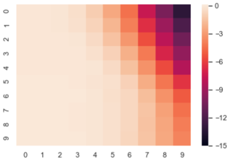
(a) GMF-Q.

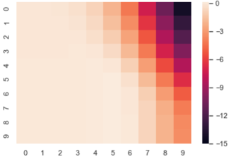
(b) GMF-V.

Figure 1: Q-tables: GMF-Q vs. GMF-V.

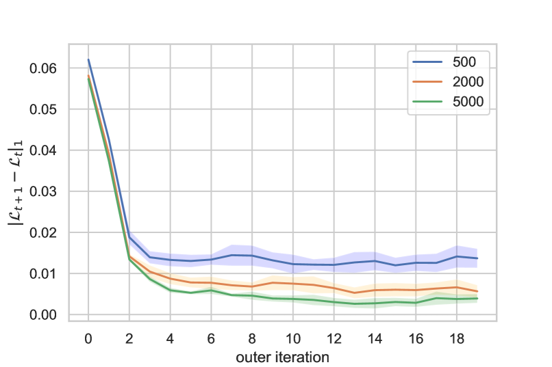
Figure 2: Convergence with different
                                                                                                                                    number of inner iterations.

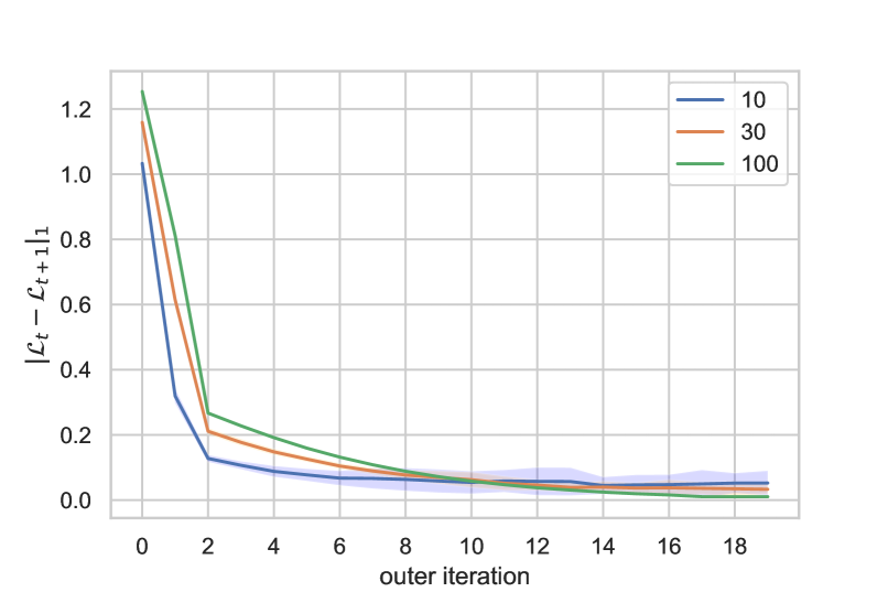
Figure 3: Convergence with different
                                                                                                                                   number of states.

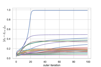
(a) fluctuation in $l_{\infty}$.

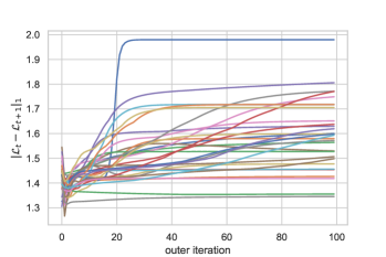
(b) fluctuation in $l_{1}$.

Figure 4: Fluctuations of Naive Algorithm (30 sample paths).

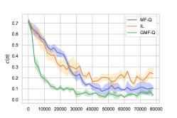
(a) $|\mathcal{S}|=|\mathcal{A}|=10,{\color[rgb]{0,0,0}N}=20$.

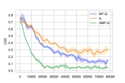
(b) $|\mathcal{S}|=|\mathcal{A}|=20,{\color[rgb]{0,0,0}N}=20$.

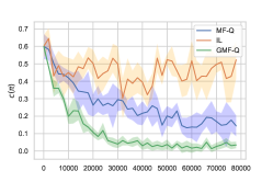
(c) $|\mathcal{S}|=|\mathcal{A}|=10,{\color[rgb]{0,0,0}N}=40$.

Figure 5: Learning accuracy based on $C(\boldsymbol{\pi})$.

Comparison with existing algorithms for $N$-player games.

To test the effectiveness of GMF-Q for approximating $N$-player games, we next compare GMF-Q with IL algorithm and MF-Q algorithm. IL algorithm T1993 considers $N$ independent players and each player solves a decentralized reinforcement learning problem ignoring other players in the system. The MF-Q algorithm YLLZZW2018 extends the NASH-Q Learning algorithm for the $N$-player game introduced in HW2003 , adds the aggregate actions $(\bar{\boldsymbol{a}}_{-i}=\frac{\sum_{j\neq i}a_{j}}{{\color[rgb]{0,0,0}N}-1})$ from the opponents, and works for the class of games where the interactions are only through the average actions of $N$ players.

Performance metric.

We adopt the following metric to measure the difference between a given policy $\pi$ and an NE (here $\epsilon_{0}>0$ is a safeguard, and is taken as $0.1$ in the experiments):

$$C(\boldsymbol{\pi})=\frac{1}{N|\mathcal{S}|^{N}}\sum\nolimits_{i=1}^{N}\sum\nolimits_{\boldsymbol{s}\in\mathcal{S}^{N}}\dfrac{\max_{{\pi}^{i}}V_{i}(\boldsymbol{s},({\boldsymbol{\pi}^{-i}},\pi^{i}))-V_{i}(\boldsymbol{s},{\boldsymbol{\pi}})}{|\max_{{\pi}^{i}}V_{i}(\boldsymbol{s},({\boldsymbol{\pi}^{-i}},\pi^{i}))|+\epsilon_{0}}.$$

Clearly $C(\boldsymbol{\pi})\geq 0$, and $C(\boldsymbol{\pi}^{*})=0$ if and only if $\boldsymbol{\pi}^{*}$ is an NE. Policy $\arg\max_{{\pi}_{i}}V_{i}(\boldsymbol{s},({\boldsymbol{\pi}^{-i}},\pi_{i}))$ is called the best response to $\boldsymbol{\pi}^{-i}$. A similar metric without normalization has been adopted in PPP2018 .

Our experiment (Figure 5) shows that GMF-Q is superior in terms of convergence rate, accuracy, and stability for approximating an $N$-player game: GMF-Q converges faster than IL and MF-Q, with the smallest error, and with the lowest variance, as $\epsilon$-net improves the stability.

For instance, when $N=20$, IL Algorithm converges with the largest error $0.220$. The error from MF-Q is $0.101$, smaller than IL but still bigger than the error from GMF-Q. The GMF-Q converges with the lowest error $0.065$. Moreover, as $N$ increases, the error of GMF-Q deceases while the errors of both MF-Q and IL increase significantly. As $|\mathcal{S}|$ and $|\mathcal{A}|$ increase, GMF-Q is robust with respect to this increase of dimensionality, while both MF-Q and IL clearly suffer from the increase of the dimensionality with decreased convergence rate and accuracy. Therefore, GMF-Q is more scalable than IL and MF-Q, when the system is complex and the number of players $N$ is large.

6 Conclusion

This paper builds a GMFG framework for simultaneous learning and decision-making, establishes the existence and uniqueness of NE, and proposes a Q-learning algorithm GMF-Q with convergence and complexity analysis. Experiments demonstrate superior performance of GMF-Q.

Appendix A Distance metrics and completeness

This section reviews some basic properties of the Wasserstein distance. It then proves that the metrics defined in the main text are indeed distance functions and define complete metric spaces.

$\ell_{1}$-Wasserstein distance and dual representation.

The $\ell_{1}$ Wasserstein distance over $\mathcal{P}(\mathcal{X})$ for $\mathcal{X}\subseteq\mathbb{R}^{k}$ is defined as

$$W_{1}(\nu,\nu^{\prime}):=\inf_{M\in\mathcal{M}(\nu,\nu^{\prime})}\int_{\mathcal{X}\times\mathcal{X}}\|x-y\|_{2}\text{d}M(x,y).$$ (13)

where $\mathcal{M}(\nu,\nu^{\prime})$ is the set of all measures (couplings) on $\mathcal{X}\times\mathcal{X}$, with marginals $\nu$ and $\nu^{\prime}$ on the two components, respectively.

The Kantorovich duality theorem enables the following equivalent dual representation of $W_{1}$:

$$W_{1}(\nu,\nu^{\prime})=\sup_{\|f\|_{L}\leq 1}\left|\int_{\mathcal{X}}fd\nu-\int_{\mathcal{X}}fd\nu^{\prime}\right|,$$ (14)

where the supremum is taken over all $1$-Lipschitz functions $f$, i.e., $f$ satisfying $|f(x)-f(y)|\leq\|x-y\|_{2}$ for all $x,y\in\mathcal{X}$.

The Wasserstein distance $W_{1}$ can also be related to the total variation distance via the following inequalities [9]:

$$d_{\min}(\mathcal{X})d_{TV}(\nu,\nu^{\prime})\leq W_{1}(\nu,\nu^{\prime})\leq\text{diam}(\mathcal{X})d_{TV}(\nu,\nu^{\prime}),$$ (15)

where $d_{\min}(\mathcal{X})=\min_{x\neq y\in\mathcal{X}}\|x-y\|_{2}$, which is guaranteed to be positive when $\mathcal{X}$ is finite.

When $\mathcal{S}$ and $\mathcal{A}$ are compact, for any compact subset $\mathcal{X}\subseteq\mathbb{R}^{k}$, and for any $\nu,\nu^{\prime}\in\mathcal{P}(\mathcal{X})$, $W_{1}(\nu,\nu^{\prime})\leq\text{diam}(\mathcal{X})d_{TV}(\nu,\nu^{\prime})\leq\text{diam}(\mathcal{X})<\infty$, where $\text{diam}(\mathcal{X})=\sup_{x,y\in\mathcal{X}}\|x-y\|_{2}$ and $d_{TV}$ is the total variation distance. Moreover, one can verify

Lemma 3.

Both $D$ and $\mathcal{W}_{1}$ are distance functions, and they are finite for any input distribution pairs. In addition, both $(\{\Pi\}_{t=0}^{\infty},D)$ and $(\{\mathcal{P}(\mathcal{S}\times\mathcal{A})\}_{t=0}^{\infty},\mathcal{W}_{1})$ are complete metric spaces.

These facts enable the usage of Banach fixed-point mapping theorem for the proof of existence and uniqueness (Theorems 1 and 4).

Proof of Lemma 3.

It is known that for any compact set $\mathcal{X}\subseteq\mathbb{R}^{k}$, $(\mathcal{P}(\mathcal{X}),W_{1})$ defines a complete metric space [5]. Since $W_{1}(\nu,\nu^{\prime})\leq\text{diam}(\mathcal{X})$ is uniformly bounded for any $\nu,~{}\nu^{\prime}\in\mathcal{P}(\mathcal{X})$, we know that $\mathcal{W}_{1}(\boldsymbol{\mathcal{L}},\boldsymbol{\mathcal{L}}^{\prime})\leq\text{diam}(\mathcal{X})$ and $D(\boldsymbol{\pi},\boldsymbol{\pi^{\prime}})\leq\text{diam}(\mathcal{X})$ as well, so they are both finite for any input distribution pairs. It is clear that they are distance functions based on the fact that $W_{1}$ is a distance function.

Finally, we show the completeness of the two metric spaces $(\{\Pi\}_{t=0}^{\infty},D)$ and $(\{\mathcal{P}(\mathcal{S}\times\mathcal{A})\}_{t=0}^{\infty},\mathcal{W}_{1})$. Take $(\{\Pi\}_{t=0}^{\infty},D)$ for example. Suppose that $\boldsymbol{\pi}^{k}$ is a Cauchy sequence in $(\{\Pi\}_{t=0}^{\infty},D)$. Then for any $\epsilon>0$, there exists a positive integer $N$, such that for any $m,~{}n\geq N$,

$$D(\boldsymbol{\pi}^{n},\boldsymbol{\pi}^{m})\leq\epsilon\Longrightarrow W_{1}(\pi_{t}^{n}(s),\pi_{t}^{m}(s))\leq\epsilon\text{ for any $s\in\mathcal{S}$, $t\in\mathbb{N}$},$$ (16)

which implies that $\pi_{t}^{k}(s)$ forms a Cauchy sequence in $(\mathcal{P}(\mathcal{A}),W_{1})$, and hence by the completeness of $(\mathcal{P}(\mathcal{A}),W_{1})$, $\pi_{t}^{k}(s)$ converges to some $\pi_{t}(s)\in\mathcal{P}(\mathcal{A})$. As a result, $\boldsymbol{\pi}^{n}\rightarrow\boldsymbol{\pi}\in\{\Pi\}_{t=0}^{\infty}$ under metric $D$, which shows that $(\{\Pi\}_{t=0}^{\infty},D)$ is complete.

The completeness of $(\{\mathcal{P}(\mathcal{S}\times\mathcal{A})\}_{t=0}^{\infty},\mathcal{W}_{1})$ can be proved similarly. ∎

The same argument for Lemma 3 shows that both $D$ and $W_{1}$ are distance functions and are finite for any input distribution pairs, with both $(\Pi,D)$ and $(\mathcal{P}(\mathcal{S}\times\mathcal{A}),W_{1})$ again complete metric spaces.

Appendix B Existence and uniqueness for stationary NE of GMFGs

Definition B.1 (Stationary NE for GMFGs).

In (GMFG), a player-population profile ($\pi^{\star}$, $\mathcal{L}^{\star}$) is called a stationary NE if

1. (Single player side) For any policy $\pi$ and any initial state $s\in\mathcal{S}$,

   $$V\left(s,\pi^{\star},{\color[rgb]{0,0,0}\mathcal{L}^{\star}}\right)\geq V\left(s,\pi,{\color[rgb]{0,0,0}\mathcal{L}^{\star}}\right).$$ (17)

2. (Population side) $\mathbb{P}_{s_{t},a_{t}}={\mathcal{L}^{\star}}$ for all $t\geq 0$, where $\{s_{t},a_{t}\}_{t=0}^{\infty}$ is the dynamics under the policy $\pi^{\star}$ starting from $s_{0}\sim\mu^{\star}$, with $a_{t}\sim\pi^{\star}(s_{t},{\color[rgb]{0,0,0}\mu^{\star}})$, $s_{t+1}\sim P(\cdot|s_{t},a_{t},{\color[rgb]{0,0,0}\mathcal{L}^{\star}})$, and $\mu^{\star}$ being the population state marginal of $\mathcal{L}^{\star}$.

The existence and uniqueness of the NE to (GMFG) in the stationary setting can be established by modifying appropriately the same fixed-point approach for the GMFG in the main text.

Step 1.

Fix $\mathcal{L}$, the GMFG becomes the classical optimization problem. That is, solving (GMFG) is now reduced to finding a policy $\pi_{\mathcal{L}}^{\star}\in\Pi:=\{\pi\,|\,\pi:\mathcal{S}\rightarrow\mathcal{P}(\mathcal{A})\}$ to maximize

$$\begin{array}[]{ll}V(s,\pi_{\mathcal{L}},\mathcal{L}):=&\mathbb{E}\left[\sum\limits_{t=0}^{\infty}\gamma^{t}r(s_{t},a_{t},\mathcal{L})|s_{0}=s\right],\\ \text{subject to}&s_{t+1}\sim P(s_{t},a_{t},\mathcal{L}),\quad a_{t}\sim\pi_{\mathcal{L}}(s_{t}).\end{array}$$

Now given this fixed $\mathcal{L}$ and the solution $\pi_{\mathcal{L}}^{\star}$ to the above optimization problem, one can again define

$$\Gamma_{1}:\mathcal{P}(\mathcal{S}\times\mathcal{A})\rightarrow\Pi,$$

such that $\pi_{\mathcal{L}}^{\star}=\Gamma_{1}(\mathcal{L})$. Note that this $\pi_{\mathcal{L}}^{\star}$ satisfies the single player side condition for the population state-action pair $L$,

$$V\left(s,\pi_{\mathcal{L}}^{\star},\mathcal{L}\right)\geq V\left(s,\pi,\mathcal{L}\right),$$ (18)

for any policy $\pi$ and any initial state $s\in\mathcal{S}$.

Accordingly, a similar feedback regularity condition is needed in this step.

Assumption 3.

There exists a constant $d_{1}\geq 0$, such that for any $\mathcal{L},\mathcal{L}^{\prime}\in\mathcal{P}(\mathcal{S}\times\mathcal{A})$,

$$D(\Gamma_{1}(\mathcal{L}),\Gamma_{1}(\mathcal{L}^{\prime}){\color[rgb]{0,0,0})}\leq d_{1}W_{1}(\mathcal{L},\mathcal{L}^{\prime}),$$ (19)

where

$$\begin{split}D(\pi,\pi^{\prime})&:=\sup_{s\in\mathcal{S}}W_{1}(\pi(s),\pi^{\prime}(s)),\end{split}$$ (20)

and $W_{1}$ is the $\ell_{1}$-Wasserstein distance (a.k.a. earth mover distance) between probability measures.

Step 2.

Based on the analysis of Step 1 and $\pi_{\mathcal{L}}^{\star}$, update the initial $\mathcal{L}$ to $\mathcal{L}^{\prime}$ following the controlled dynamics $P(\cdot|s_{t},a_{t},\mathcal{L})$.

Accordingly, define a mapping $\Gamma_{2}:\Pi\times\mathcal{P}(\mathcal{S}\times\mathcal{A})\rightarrow\mathcal{P}(\mathcal{S}\times\mathcal{A})$ as follows:

$$\Gamma_{2}(\pi,\mathcal{L}):=\hat{\mathcal{L}}=\mathbb{P}_{s_{1},a_{1}},$$ (21)

where $a_{1}\sim\pi(s_{1})$, $s_{1}\sim\mu P(\cdot|\cdot,a_{0},\mathcal{L})$, $a_{0}\sim\pi(s_{0})$, $s_{0}\sim\mu$, and $\mu$ is the population state marginal of $\mathcal{L}$.

One also needs a similar assumption in this step.

Assumption 4.

There exist constants $d_{2},~{}d_{3}\geq 0$, such that for any admissible policies $\pi,\pi_{1},\pi_{2}$ and joint distributions $\mathcal{L},\mathcal{L}_{1},\mathcal{L}_{2}$,

$$W_{1}(\Gamma_{2}(\pi_{1},\mathcal{L}),\Gamma_{2}(\pi_{2},\mathcal{L}))\leq d_{2}D(\pi_{1},\pi_{2}),\\$$ (22)

$$W_{1}(\Gamma_{2}(\pi,\mathcal{L}_{1}),\Gamma_{2}(\pi,\mathcal{L}_{2}))\leq d_{3}W_{1}(\mathcal{L}_{1},\mathcal{L}_{2}).$$ (23)

Step 3.

Repeat until $\mathcal{L}^{\prime}$ matches $\mathcal{L}$.

This step is to ensure the population side condition. To ensure the convergence of the combined step one and step two, it suffices if $\Gamma:\mathcal{P}(\mathcal{S}\times\mathcal{A})\rightarrow\mathcal{P}(\mathcal{S}\times\mathcal{A})$ with $\Gamma(\mathcal{L}):=\Gamma_{2}(\Gamma_{1}(\mathcal{L}),\mathcal{L})$ is a contractive mapping (under the $W_{1}$ distance).

Similar to the proof of Theorem 1, again by the Banach fixed point theorem and the completeness of the related metric spaces, there exists a unique stationary NE of the GMFG. That is,

Theorem 4 (Existence and Uniqueness of stationary MFG solution).

Given Assumptions 3 and 4, and assume $d_{1}d_{2}+d_{3}<1$. Then there exists a unique stationary NE to (GMFG).

Appendix C Additional comments on assumptions

As mentioned in the main text, the single player side Assumption 1 and its counterpart Assumption 3 for the stationary version correspond to the feedback regularity condition in the classical MFG literature. Here we add some comments on the population side Assumption 2 and its stationary version Assumption 4. For simplicity and clarity, let us consider the stationary case with finite state and action spaces. Then we have the following result.

Lemma 5.

Suppose that $\max_{s,a,\mathcal{L},s^{\prime}}P(s^{\prime}|s,a,\mathcal{L})\leq c_{1}$, and that $P(s^{\prime}|s,a,\cdot)$ is $c_{2}$-Lipschitz in $W_{1}$, i.e.,

$$|P(s^{\prime}|s,a,\mathcal{L}_{1})-P(s^{\prime}|s,a,\mathcal{L}_{2})|\leq c_{2}W_{1}(\mathcal{L}_{1},\mathcal{L}_{2}).$$ (24)

Then in Assumption 4, $d_{2}$ and $d_{3}$ can be chosen as

$$d_{2}=\frac{2\text{diam}(\mathcal{S})\text{diam}(\mathcal{A})|\mathcal{S}|c_{1}}{d_{\min}(\mathcal{A})}$$ (25)

and $d_{3}=\frac{\text{diam}(\mathcal{S})\text{diam}(\mathcal{A})c_{2}}{2}$, respectively.

Lemma 5 provides an explicit characterization of the population side assumptions based only on the boundedness and Lipschitz properties of the transition dynamics $P$. In particular, $c_{1}$ becomes smaller when the transition dynamics becomes more diverse and the state space becomes larger.

Proof.

(Lemma 5) We begin by noticing that $\mathcal{L}^{\prime}=\Gamma_{2}(\pi,\mathcal{L})$ can be expanded and computed as follows:

$$\mu^{\prime}(s^{\prime})=\sum\nolimits_{s\in\mathcal{S},a\in\mathcal{A}}\mu(s)P(s^{\prime}|s,a,\mathcal{L})\pi(s,a),\quad\mathcal{L}^{\prime}(s^{\prime},a^{\prime})=\mu^{\prime}(s^{\prime})\pi(s^{\prime},a^{\prime}),$$ (26)

where $\mu$ is the state marginal distribution of $\mathcal{L}$.

Now by the inequalities (15), we have

$$\begin{split}W_{1}&(\Gamma_{2}(\pi_{1},\mathcal{L}),\Gamma_{2}(\pi_{2},\mathcal{L}))\leq\text{diam}(\mathcal{S}\times\mathcal{A})d_{TV}(\Gamma_{2}(\pi_{1},\mathcal{L}),\Gamma_{2}(\pi_{2},\mathcal{L}))\\ =&\dfrac{\text{diam}(\mathcal{S}\times\mathcal{A})}{2}\sum_{s^{\prime}\in\mathcal{S},a^{\prime}\in\mathcal{A}}\left|\sum_{s\in\mathcal{S},a\in\mathcal{A}}\mu(s)P(s^{\prime}|s,a,\mathcal{L})\left(\pi_{1}(s,a)\pi_{1}(s^{\prime},a^{\prime})-\pi_{2}(s,a)\pi_{2}(s^{\prime},a^{\prime})\right)\right|\\ \leq&\dfrac{\text{diam}(\mathcal{S}\times\mathcal{A})}{2}\max_{s,a,\mathcal{L},s^{\prime}}P(s^{\prime}|s,a,\mathcal{L})\sum_{s,a,s^{\prime},a^{\prime}}\mu(s)(\pi_{1}(s,a)+\pi_{2}(s,a))|\pi_{1}(s^{\prime},a^{\prime})-\pi_{2}(s^{\prime},a^{\prime})|\\ \leq&\dfrac{\text{diam}(\mathcal{S}\times\mathcal{A})}{2}\max_{s,a,\mathcal{L},s^{\prime}}P(s^{\prime}|s,a,\mathcal{L})\sum_{s^{\prime},a^{\prime}}|\pi_{1}(s^{\prime},a^{\prime})-\pi_{2}(s^{\prime},a^{\prime})|\cdot(1+1)\\ =&2\text{diam}(\mathcal{S}\times\mathcal{A})\max_{s,a,\mathcal{L},s^{\prime}}P(s^{\prime}|s,a,\mathcal{L})\sum_{s^{\prime}}d_{TV}(\pi_{1}(s^{\prime}),\pi_{2}(s^{\prime}))\\ \leq&\frac{2\text{diam}(\mathcal{S}\times\mathcal{A})\max_{s,a,\mathcal{L},s^{\prime}}P(s^{\prime}|s,a,\mathcal{L})|\mathcal{S}|}{d_{\min}(\mathcal{A})}D(\pi_{1},\pi_{2})=\frac{2\text{diam}(\mathcal{S})\text{diam}(\mathcal{A})|\mathcal{S}|c_{1}}{d_{\min}(\mathcal{A})}D(\pi_{1},\pi_{2}).\end{split}$$ (27)

Similarly, we have

$$\begin{split}W_{1}&(\Gamma_{2}(\pi,\mathcal{L}_{1}),\Gamma_{2}(\pi,\mathcal{L}_{2}))\leq\text{diam}(\mathcal{S}\times\mathcal{A})d_{TV}(\Gamma_{2}(\pi,\mathcal{L}_{1}),\Gamma_{2}(\pi,\mathcal{L}_{2}))\\ =&\dfrac{\text{diam}(\mathcal{S}\times\mathcal{A})}{2}\sum_{s^{\prime}\in\mathcal{S},a^{\prime}\in\mathcal{A}}\left|\sum_{s\in\mathcal{S},a\in\mathcal{A}}\mu(s)\pi(s,a)\pi(s^{\prime},a^{\prime})\left(P(s^{\prime}|s,a,\mathcal{L}_{1})-P(s^{\prime}|s,a,\mathcal{L}_{2})\right)\right|\\ \leq&\dfrac{\text{diam}(\mathcal{S}\times\mathcal{A})}{2}\sum_{s,a,s^{\prime},a^{\prime}}\mu(s)\pi(s,a)\pi(s^{\prime},a^{\prime})\left|P(s^{\prime}|s,a,\mathcal{L}_{1})-P(s^{\prime}|s,a,\mathcal{L}_{2})\right|\\ \leq&\frac{\text{diam}(\mathcal{S})\text{diam}(\mathcal{A})c_{2}}{2}.\end{split}$$ (28)

This completes the proof. ∎

Appendix D Proof of Theorems 1 and 4

For notational simplicity, we only present the proof for the stationary case (Theorem 4). The proof of Theorems 1 is the same with appropriate notational changes.

First by Definition B.1 and the definitions of $\Gamma_{i}$ $(i=1,2)$, $(\pi,\mathcal{L})$ is a stationary NE iff $\mathcal{L}=\Gamma(\mathcal{L})=\Gamma_{2}(\Gamma_{1}(\mathcal{L}),\mathcal{L})$ and $\pi=\Gamma_{1}(\mathcal{L})$, where $\Gamma(\mathcal{L})=\Gamma_{2}(\Gamma_{1}(\mathcal{L}),\mathcal{L})$. This indicates that for any $\mathcal{L}_{1},\mathcal{L}_{2}\in\mathcal{P}(\mathcal{S}\times\mathcal{A})$,

$$\begin{split}&W_{1}(\Gamma(\mathcal{L}_{1}),\Gamma(\mathcal{L}_{2}))=W_{1}(\Gamma_{2}(\Gamma_{1}(\mathcal{L}_{1}),\mathcal{L}_{1}),\Gamma_{2}(\Gamma_{1}(\mathcal{L}_{2}),\mathcal{L}_{2}))\\ &\leq W_{1}(\Gamma_{2}(\Gamma_{1}(\mathcal{L}_{1}),\mathcal{L}_{1}),\Gamma_{2}(\Gamma_{1}(\mathcal{L}_{2}),\mathcal{L}_{1}))+W_{1}(\Gamma_{2}(\Gamma_{1}(\mathcal{L}_{2}),\mathcal{L}_{1}),\Gamma_{2}(\Gamma_{1}(\mathcal{L}_{2}),\mathcal{L}_{2}))\\ &\leq(d_{1}d_{2}+d_{3})W_{1}(\mathcal{L}_{1},\mathcal{L}_{2}).\end{split}$$ (29)

And since $d_{1}d_{2}+d_{3}\in[0,1)$, by the Banach fixed-point theorem, we conclude that there exists a unique fixed-point of $\Gamma$, or equivalently, a unique stationary MFG solution to (GMFG).

Appendix E Proof of Theorem 2

The proof of Theorem 2 relies on the following lemmas.

Lemma 6 ([8]).

The softmax function is $c$-Lipschitz, i.e., $\|\textbf{softmax}_{c}(x)-\textbf{softmax}_{c}(y)\|_{2}\leq c\|x-y\|_{2}$ for any $x,~{}y\in\mathbb{R}^{n}$.

Notice that for a finite set $\mathcal{X}\subseteq\mathbb{R}^{k}$ and any two (discrete) distributions $\nu,~{}\nu^{\prime}$ over $\mathcal{X}$, we have

$$\begin{split}W_{1}(\nu,\nu^{\prime})&\leq\text{diam}(\mathcal{X})d_{TV}(\nu,\nu^{\prime})=\frac{\text{diam}(\mathcal{X})}{2}\|\nu-\nu^{\prime}\|_{1}\leq\frac{\text{diam}(\mathcal{X})}{2}\|\nu-\nu^{\prime}\|_{2},\end{split}$$ (30)

where in computing the $\ell_{1}$-norm, $\nu,~{}\nu^{\prime}$ are viewed as vectors of length $|\mathcal{X}|$.

Hence Lemma 6 implies that for any $x,~{}y\in\mathbb{R}^{|\mathcal{X}|}$, when $\textbf{softmax}_{c}(x)$ and $\textbf{softmax}_{c}(y)$ are viewed as probability distributions over $\mathcal{X}$, we have

$$W_{1}(\textbf{softmax}_{c}(x),\textbf{softmax}_{c}(y))\leq\frac{\text{diam}(\mathcal{X})c}{2}\|x-y\|_{2}\leq\frac{\text{diam}(\mathcal{X})\sqrt{|\mathcal{X}|}c}{2}\|x-y\|_{\infty}.$$

Lemma 7.

The distance between the softmax and the argmax mapping is bounded by

$$\|\textbf{softmax}_{c}(x)-\textbf{argmax-e}(x)\|_{2}\leq 2n\exp(-c\delta),$$

where $\delta=x_{\max}-\max_{x_{j}<x_{\max}}x_{j}$, $x_{\max}=\max_{i=1,\dots,n}x_{i}$, and $\delta:=\infty$ when all $x_{j}$ are equal.

Similar to Lemma 6, Lemma 7 implies that for any $x\in\mathbb{R}^{|\mathcal{X}|}$, viewing $\textbf{softmax}_{c}(x)$ as probability distributions over $\mathcal{X}$ leads to

$$W_{1}(\textbf{softmax}_{c}(x),\textbf{argmax-e}(x))\leq\text{diam}(\mathcal{X})|\mathcal{X}|\exp(-c\delta).$$

Proof of Lemma 7.

Without loss of generality, assume that $x_{1}=x_{2}=\dots=x_{m}=\max_{i=1,\dots,n}x_{i}=x^{\star}>x_{j}$ for all $m<j\leq n$. Then

$$\textbf{argmax-e}(x)_{i}=\begin{cases}\frac{1}{m},&i\leq m,\\ 0,&otherwise.\end{cases}$$

$$\textbf{softmax}_{c}(x)_{i}=\begin{cases}\frac{e^{cx^{\star}}}{me^{cx^{\star}}+\sum_{j=m+1}^{n}e^{cx_{j}}},&i\leq m,\\ \frac{e^{cx_{i}}}{me^{cx^{\star}}+\sum_{j=m+1}^{n}e^{cx_{j}}},&otherwise.\end{cases}$$

Therefore

$$\begin{split}\|\textbf{soft}&\textbf{max}_{c}(x)-\textbf{argmax-e}(x)\|_{2}\leq\|\textbf{softmax}_{c}(x)-\textbf{argmax-e}(x)\|_{1}\\ =&m\left(\frac{1}{m}-\frac{e^{cx^{\star}}}{me^{cx^{\star}}+\sum_{j=m+1}^{n}e^{cx_{j}}}\right)+\frac{\sum_{i=m+1}^{n}e^{cx_{i}}}{me^{cx^{\star}}+\sum_{j=m+1}^{n}e^{cx_{j}}}\\ =&\frac{2\sum_{i=m+1}^{n}e^{cx_{i}}}{me^{cx^{\star}}+\sum_{i=m+1}^{n}e^{cx_{i}}}=\frac{2\sum_{i=m+1}^{n}e^{-c\delta_{i}}}{m+\sum_{i=m+1}^{n}e^{-c\delta_{i}}}\\ \leq&\frac{2}{m}\sum_{i=m+1}^{n}e^{-c\delta_{i}}\leq\frac{2(n-m)}{m}e^{-c\delta}\leq 2ne^{-c\delta},\end{split}$$

with $\delta_{i}=x_{i}-x^{\star}$. ∎

Lemma 8 ([7]).

For an MDP, say $\mathcal{M}$, suppose that the Q-learning algorithm takes step-sizes

$$\beta_{t}(s,a)=\begin{cases}|\#(s,a,t)+1|^{-h},&(s,a)=(s_{t},a_{t}),\\ 0,&\text{otherwise}.\end{cases}$$

with $h\in(1/2,1)$. Here $\#(s,a,t)$ is the number of times up to time $t$ that one visits the state-action pair $(s,a)$. Also suppose that the covering time of the state-action pairs is bounded by $L$ with probability at least $1-p$ for some $p\in(0,1)$. Then $\|Q_{T^{\mathcal{M}}(\delta,\epsilon)}-Q^{\star}\|_{\infty}\leq\epsilon$ with probability at least $1-2\delta$. Here $Q_{T}$ is the $T$-th update in Q-learning, and $Q^{\star}$ is the (optimal) Q-function, given that

$$\begin{split}T^{\mathcal{M}}(\delta,&\epsilon)=\Omega\left(\left(\dfrac{L\log_{p}(\delta)}{\beta}\log\dfrac{V_{\max}}{\epsilon}\right)^{\frac{1}{1-h}}+\left(\dfrac{\left(L\log_{p}(\delta)\right)^{1+3h}V_{\max}^{2}\log\left(\frac{|\mathcal{S}||\mathcal{A}|V_{\max}}{\delta\beta\epsilon}\right)}{\beta^{2}\epsilon^{2}}\right)^{\frac{1}{h}}\right),\end{split}$$

where $\beta=(1-\gamma)/2$, $V_{\max}=R_{\max}/(1-\gamma)$, and $R_{\max}$ is an upper bound on the extreme difference between the expected rewards, i.e., $\max_{s,a,\mu}{r}(s,a,\mu)-\min_{s,a,\mu}{r}(s,a,\mu)\leq R_{\max}$.

Here the covering time $L$ of a state-action pair sequence is defined to be the number of steps needed to visit all state-action pairs starting from any arbitrary state-action pair, and $T^{\mathcal{M}}(\delta,\epsilon)$ is the number of inner iterations $T_{k}$ set in Algorithm 1. This will guarantee the convergence in Theorem 2. Also notice that the $l_{\infty}$ norm above is defined in an element-wise sense, i.e., for $M\in\mathbb{R}^{|\mathcal{S}|\times|\mathcal{A}|}$, we have $\|M\|_{\infty}=\max_{s\in\mathcal{S},a\in\mathcal{A}}|M(s,a)|$.

Proof of Theorem 2.

Define $\hat{\Gamma}_{1}^{k}(\mathcal{L}_{k}):=\textbf{softmax}_{c}\left(\hat{Q}^{\star}_{\mathcal{L}_{k}}\right)$. In the following, $\pi=\textbf{softmax}_{c}(Q_{\mathcal{L}})$ is understood as the policy $\pi$ with $\pi(s)=\textbf{softmax}_{c}(Q_{\mathcal{L}}(s,\cdot))$. Let $\mathcal{L}^{\star}$ be the population state-action pair in a stationary NE of (GMFG). Then $\pi_{k}=\hat{\Gamma}_{1}^{k}(\mathcal{L}_{k})$. Denoting $d:=d_{1}d_{2}+d_{3}$, we see

$$\begin{split}W_{1}(\tilde{\mathcal{L}}_{k+1}&,\mathcal{L}^{\star})=W_{1}(\Gamma_{2}(\pi_{k},\mathcal{L}_{k}),\Gamma_{2}(\Gamma_{1}(\mathcal{L}^{\star}),\mathcal{L}^{\star}))\\ \leq&W_{1}(\Gamma_{2}(\Gamma_{1}(\mathcal{L}_{k}),\mathcal{L}_{k}),\Gamma_{2}(\Gamma_{1}(\mathcal{L}^{\star}),\mathcal{L}^{\star}))+W_{1}(\Gamma_{2}(\Gamma_{1}(\mathcal{L}_{k}),\mathcal{L}_{k}),\Gamma_{2}(\hat{\Gamma}_{1}^{k}(\mathcal{L}_{k}),\mathcal{L}_{k}))\\ \leq&W_{1}(\Gamma(\mathcal{L}_{k}),\Gamma(\mathcal{L}^{\star}))+d_{2}D(\Gamma_{1}(\mathcal{L}_{k}),\hat{\Gamma}_{1}^{k}(\mathcal{L}_{k}))\\ \leq&(d_{1}d_{2}+d_{3})W_{1}(\mathcal{L}_{k},\mathcal{L}^{\star})+d_{2}D(\textbf{argmax-e}(Q_{\mathcal{L}_{k}}^{\star}),\textbf{softmax}_{c}(\hat{Q}_{\mathcal{L}_{k}}^{\star}))\\ \leq&dW_{1}(\mathcal{L}_{k},\mathcal{L}^{\star})+d_{2}D(\textbf{softmax}_{c}(\hat{Q}_{\mathcal{L}_{k}}^{\star}),\textbf{softmax}_{c}(Q_{\mathcal{L}_{k}}^{\star}))\\ &+d_{2}D(\textbf{argmax-e}(Q_{\mathcal{L}_{k}}^{\star}),\textbf{softmax}_{c}(Q_{\mathcal{L}_{k}}^{\star}))\\ \leq&dW_{1}(\mathcal{L}_{k},\mathcal{L}^{\star})+\frac{cd_{2}\text{diam}(\mathcal{A})\sqrt{|\mathcal{A}|}}{2}\|\hat{Q}_{\mu_{k}}^{\star}-Q_{\mu_{k}}^{\star}\|_{\infty}\\ &+d_{2}D(\textbf{argmax-e}(Q_{\mathcal{L}_{k}}^{\star}),\textbf{softmax}_{c}(Q_{\mathcal{L}_{k}}^{\star})).\end{split}$$

Then since $\mathcal{L}_{k}\in S_{\epsilon}$ by the projection step, Lemma 7, and Lemma 8 with the choice of $T_{k}=T^{\mathcal{M}_{\mu}}(\delta_{k},\epsilon_{k})$), we have, with probability at least $1-2\delta_{k}$,

$$W_{1}(\tilde{\mathcal{L}}_{k+1},\mathcal{L}^{\star})\leq dW_{1}(\mathcal{L}_{k},\mathcal{L}^{\star})+\frac{cd_{2}\text{diam}(\mathcal{A})\sqrt{|\mathcal{A}|}}{2}\epsilon_{k}+d_{2}\text{diam}(\mathcal{A})|\mathcal{A}|e^{-c\phi(\epsilon)}.$$ (31)

Finally, it is clear that with probability at least $1-2\delta_{k}$,

$$\begin{split}W_{1}(\mathcal{L}_{k+1},\mathcal{L}^{\star})&\leq W_{1}(\tilde{\mathcal{L}}_{k+1},\mathcal{L}^{\star})+W_{1}(\tilde{\mathcal{L}}_{k+1},\textbf{Proj}_{S_{\epsilon}}(\tilde{\mathcal{L}}_{k+1}))\\ &\leq dW_{1}(\mathcal{L}_{k},\mathcal{L}^{\star})+\frac{cd_{2}\text{diam}(\mathcal{A})\sqrt{|\mathcal{A}|}}{2}\epsilon_{k}+d_{2}\text{diam}(\mathcal{A})|\mathcal{A}|e^{-c\phi(\epsilon)}+\epsilon.\end{split}$$

By telescoping, this implies that with probability at least $1-2\sum_{k=0}^{{\color[rgb]{0,0,0}K-1}}\delta_{k}$,

$$\begin{split}W_{1}(\mathcal{L}_{K},\mathcal{L}^{\star})\leq&d^{K}W_{1}(\mathcal{L}_{0},\mathcal{L}^{\star})+\frac{cd_{2}\text{diam}(\mathcal{A})\sqrt{|\mathcal{A}|}}{2}\sum_{k=0}^{K-1}d^{K-k}\epsilon_{k}\\ &+\dfrac{(d_{2}\text{diam}(\mathcal{A})|\mathcal{A}|e^{-c\phi(\epsilon)}+\epsilon)(1-d^{\color[rgb]{0,0,0}K})}{1-d}.\end{split}$$ (32)

Since $\epsilon_{k}$ is summable, hence $\sup_{k\geq 0}\epsilon_{k}<\infty$, $\sum_{k=0}^{K-1}d^{K-k}\epsilon_{k}\leq\dfrac{\sup_{k\geq 0}\epsilon_{k}}{1-d}d^{\lfloor(K-1)/2\rfloor}+\sum_{k=\lceil(K-1)/2\rceil}^{\infty}\epsilon_{k}$.

Now plugging in $K=K_{\epsilon,\eta}$, with the choice of $\delta_{k}$ and $c=\frac{\log(1/\epsilon)}{\phi(\epsilon)}$, and noticing that $d\in[0,1)$, it is clear that with probability at least $1-2\delta$,

$$\begin{split}W_{1}(\mathcal{L}_{K_{\epsilon,\eta}},\mathcal{L}^{\star})\leq&d^{K_{\epsilon,\eta}}W_{1}(\mathcal{L}_{0},\mathcal{L}^{\star})\\ &+\frac{cd_{2}\text{diam}(\mathcal{A})\sqrt{|\mathcal{A}|}}{2}\left(\dfrac{\sup_{k\geq 0}\epsilon_{k}}{1-d}d^{\lfloor(K_{\epsilon,\eta}-1)/2\rfloor}+\sum_{k=\lceil(K_{\epsilon,\eta}-1)/2\rceil}^{\infty}\epsilon_{k}\right)\\ &+\dfrac{(d_{2}\text{diam}(\mathcal{A})|\mathcal{A}|+1)\epsilon}{1-d}.\end{split}$$ (33)

Setting $\epsilon_{k}=(k+1)^{-(1+\eta)}$, then when $K_{\epsilon,\eta}\geq 2(\log_{d}(\epsilon{\color[rgb]{0,0,0}/c})+1)$,

$$\dfrac{\sup_{k\geq 0}\epsilon_{k}}{1-d}d^{\lfloor(K_{\epsilon,\eta}-1)/2\rfloor}\leq\frac{\epsilon{\color[rgb]{0,0,0}/c}}{1-d}.$$

Similarly, when $K_{\epsilon,\eta}\geq 2(\eta\epsilon{\color[rgb]{0,0,0}/c})^{-1/\eta}$, $\sum_{k=\left\lceil\frac{K_{\epsilon,\eta}-1}{2}\right\rceil}^{\infty}\epsilon_{k}\leq\epsilon{\color[rgb]{0,0,0}/c}$.

Finally, when $K_{\epsilon,\eta}\geq\log_{d}(\epsilon/(\text{diam}(\mathcal{S})\text{diam}(\mathcal{A})))$, $d^{K_{\epsilon,\eta}}W_{1}(\mathcal{L}_{0},\mathcal{L}^{\star})\leq\epsilon$, since $W_{1}(\mathcal{L}_{0},\mathcal{L}^{\star})\leq\text{diam}(\mathcal{S}\times\mathcal{A}){\color[rgb]{0,0,0}=\text{diam}(\mathcal{S})\text{diam}(\mathcal{A})}$.

In summary, if $K_{\epsilon,\eta}=\lceil 2\max\{(\eta\epsilon{\color[rgb]{0,0,0}/c})^{-1/\eta}$, $\log_{d}(\epsilon/\max\{\text{diam}(\mathcal{S})\text{diam}(\mathcal{A}),{\color[rgb]{0,0,0}c}\})+1\}\rceil$, then with probability at least $1-2\delta$,

$$\begin{split}&W_{1}(\mathcal{L}_{K_{\epsilon,\eta}},\mathcal{L}^{\star})\leq\left(1+\frac{d_{2}\text{diam}(\mathcal{A})\sqrt{|\mathcal{A}|}(2-d)}{2(1-d)}+\dfrac{(d_{2}\text{diam}(\mathcal{A})|\mathcal{A}|+1)}{1-d}\right)\epsilon=O(\epsilon).\end{split}$$

Finally, plugging in $\epsilon_{k}$ and $\delta_{k}$ into $T^{\mathcal{M}_{L}}(\delta_{k},\epsilon_{k})$, and noticing that $k{\color[rgb]{0,0,0}\leq}K_{\epsilon,\eta}$ and $\sum_{k=0}^{K_{\epsilon,\eta}-1}(k+1)^{\alpha}\leq\frac{K_{\epsilon,\eta}^{\alpha+1}}{\alpha+1}$, we immediately arrive at

$$\begin{split}T=O&\left(\left(\log(K_{\epsilon,\eta}/\delta)\right)^{\frac{1}{1-h}}K_{\epsilon,\eta}\left(\log K_{\epsilon,\eta}\right)^{\frac{1}{1-h}}+\left(\log(K_{\epsilon,\eta}/\delta)\right)^{\frac{1}{h}+3}\frac{K_{\epsilon,\eta}^{1+\frac{2(1+\eta)}{h}}}{1+\frac{2(1+\eta)}{h}}\left(\log(K_{\epsilon,\eta}/\delta)\right)^{\frac{1}{h}}\right).\end{split}$$

By further relaxing $\eta$ to $1$ and merging the terms, (12) follows. ∎

Appendix F Naive algorithm

The Naive iterative algorithm (Algorithm 2) is to replace Step A in the three-step fixed-point approach of GMFGs with Q-learning iterations. The limitation of this Naive algorithm has been discussed in the main text (Step 1, Section 4) and empirically verified in Section 5 (Figure 4).

Algorithm 2 Alternating Q-learning for GMFGs (Naive)

1:  Input: Initial population state-action pair $L_{0}$

2:  for $k=0,1,\cdots$ do

3:     Perform Q-learning to find the Q-function $Q_{k}^{\star}(s,a)=Q_{L_{k}}^{\star}(s,a)$ of an MDP with dynamics $P_{L_{k}}(s^{\prime}|s,a)$ and rewards $r_{L_{k}}(s,a)$.

4:     Solve $\pi_{k}\in\Pi$ with $\pi_{k}(s)=\textbf{argmax-e}\left(Q_{k}^{\star}(s,\cdot)\right)$.

5:     Sample $s\sim\mu_{k}$, where $\mu_{k}$ is the population state marginal of $L_{k}$, and obtain $L_{k+1}$ from $\mathcal{G}(s,\pi_{k},L_{k})$.

6:  end for

Appendix G GMF-V

GMF-V, briefly mentioned in Section 4, is the value-iteration version of our main algorithm GMF-Q. GMF-V applies to the GMFG setting with fully known transition dynamics $P$ and rewards $r$.

Algorithm 3 Value Iteration for GMFGs (GMF-V)

1:  Input: Initial $L_{0}$, tolerance $\epsilon>0$.

2:  for $k=0,1,\cdots$ do

3:     Perform value iteration for $T_{k}$ iterations to find the approximate Q-function $Q_{L_{k}}$ and value function $V_{L_{k}}$:

4:     for $t=1,2,\cdots,T_{k}$ do

5:        for all $s\in\mathcal{S}$ and $s\in\mathcal{A}$ do

6:           $Q_{L_{k}}(s,a)\leftarrow\mathbb{E}[r(s,a,L_{k})]+\gamma\sum_{s^{\prime}}P(s^{\prime}|s,a,L_{k})V_{L_{k}}(s^{\prime})$

7:           $V_{L_{k}}(s)\leftarrow\max_{a}Q_{L_{k}}(s,a)$

8:        end for

9:     end for

10:     Compute a policy $\pi_{k}\in\Pi$: ${\hskip 28.45274pt\pi_{k}(s)=\textbf{softmax}_{c}({Q}_{L_{k}}(s,\cdot))}$.

11:     Sample $s\sim\mu_{k}$, where $\mu_{k}$ is the population state marginal of $L_{k}$, and obtain $\tilde{L}_{k+1}$ from $\mathcal{G}(s,\pi_{k},L_{k})$.

12:     Find $L_{k+1}=\textbf{Proj}_{S_{\epsilon}}(\tilde{L}_{k+1})$

13:  end for

Appendix H More details for the experiments

H.1 Competition intensity index $M$.

In the experiment, the competition index $M$ is interpreted and implemented as the number of selected players in each auction competition. That is, in each round, $M-1$ players will be randomly selected from the population to compete with the representative advertiser for the auction. Therefore, the population distribution $\mathcal{L}_{t}$, the winner indicator $w_{t}^{M}$, and second-best price $a_{t}^{M}$ all depend on $M$. This parameter $M$ is also referred to as the auction thickness in the auction literature [18].

H.2 Adjustment for Algorithm MF-Q.

For MF-Q, [40] assumes all $N$ players have a joint state $s$. In the auction experiment, we make the following adjustment for MF-Q for computational efficiency and model comparability: each player $i$ makes decision based on her own private state and table $Q^{i}$ is a functional of $s^{i}$, $a^{i}$ and $\frac{\sum_{j\neq i}a^{j}}{N-1}$.

References

- (1) B. Acciaio, J. Backhoff, and R. Carmona. Extended mean field control problems: stochastic maximum principle and transport perspective. Arxiv Preprint:1802.05754, 2018.
- (2) K. Asadi and M. L. Littman. An alternative softmax operator for reinforcement learning. In Proceedings of the 34th International Conference on Machine Learning, volume 70, pages 243–252, 2017.
- (3) M. G. Bellemare, G. Ostrovski, A. Guez, P. S. Thomas, and R. Munos. Increasing the action gap: new operators for reinforcement learning. In AAAI Conference on Artificial Intelligence, pages 1476–1483, 2016.
- (4) M. Benaim and J. Y. Le Boudec. A class of mean field interaction models for computer and communication systems. Performance evaluation, 65(11-12):823–838, 2008.
- (5) F. Bolley. Separability and completeness for the Wasserstein distance. Séminaire de Probabilités XLI, pages 371–377, 2008.
- (6) H. Cai, K. Ren, W. Zhang, K. Malialis, J. Wang, Y. Yu, and D. Guo. Real-time bidding by reinforcement learning in display advertising. In Proceedings of the Tenth ACM International Conference on Web Search and Data Mining, pages 661–670. ACM, 2017.
- (7) E. Even-Dar and Y. Mansour. Learning rates for Q-learning. Journal of Machine Learning Research, 5(Dec):1–25, 2003.
- (8) B. Gao and L. Pavel. On the properties of the softmax function with application in game theory and reinforcement learning. Arxiv Preprint:1704.00805, 2017.
- (9) A. L. Gibbs and F. E. Su. On choosing and bounding probability metrics. International Statistical Review, 70(3):419–435, 2002.
- (10) D. A. Gomes, J. Mohr, and R. R. Souza. Discrete time, finite state space mean field games. Journal de mathématiques pures et appliquées, 93(3):308–328, 2010.
- (11) R. Gummadi, P. Key, and A. Proutiere. Repeated auctions under budget constraints: Optimal bidding strategies and equilibria. In the Eighth Ad Auction Workshop, 2012.
- (12) T. Haarnoja, H. Tang, P. Abbeel, and S. Levine. Reinforcement learning with deep energy-based policies. Arxiv Preprint:1702.08165, 2017.
- (13) J. Hamari, M. Sjöklint, and A. Ukkonen. The sharing economy: Why people participate in collaborative consumption. Journal of the Association for Information Science and Technology, 67(9):2047–2059, 2016.
- (14) P. Hernandez-Leal, B. Kartal, and M. E. Taylor. Is multiagent deep reinforcement learning the answer or the question? A brief survey. Arxiv Preprint:1810.05587, 2018.
- (15) J. Hu and M. P. Wellman. Nash Q-learning for general-sum stochastic games. Journal of Machine Learning Research, 4(Nov):1039–1069, 2003.
- (16) M. Huang and Y. Ma. Mean field stochastic games with binary action spaces and monotone costs. ArXiv Preprint:1701.06661, 2017.
- (17) M. Huang, R. P. Malhamé, and P. E. Caines. Large population stochastic dynamic games: closed-loop McKean-Vlasov systems and the Nash certainty equivalence principle. Communications in Information & Systems, 6(3):221–252, 2006.
- (18) K. Iyer, R. Johari, and M. Sundararajan. Mean field equilibria of dynamic auctions with learning. ACM SIGecom Exchanges, 10(3):10–14, 2011.
- (19) S. H. Jeong, A. R. Kang, and H. K. Kim. Analysis of game bot’s behavioral characteristics in social interaction networks of MMORPG. ACM SIGCOMM Computer Communication Review, 45(4):99–100, 2015.
- (20) J. Jin, C. Song, H. Li, K. Gai, J. Wang, and W. Zhang. Real-time bidding with multi-agent reinforcement learning in display advertising. Arxiv Preprint:1802.09756, 2018.
- (21) S. Kapoor. Multi-agent reinforcement learning: A report on challenges and approaches. Arxiv Preprint:1807.09427, 2018.
- (22) A. C Kizilkale and P. E Caines. Mean field stochastic adaptive control. IEEE Transactions on Automatic Control, 58(4):905–920, 2013.
- (23) J-M. Lasry and P-L. Lions. Mean field games. Japanese Journal of Mathematics, 2(1):229–260, 2007.
- (24) C-A. Lehalle and C. Mouzouni. A mean field game of portfolio trading and its consequences on perceived correlations. ArXiv Preprint:1902.09606, 2019.
- (25) J. P. M. López. Discrete time mean field games: The short-stage limit. Journal of Dynamics & Games, 2(1):89–101, 2015.
- (26) D. Mguni, J. Jennings, and E. M. de Cote. Decentralised learning in systems with many, many strategic agents. In Thirty-Second AAAI Conference on Artificial Intelligence, 2018.
- (27) V. M. Minh, A. P. Badia, M. Mirza, A. Graves, T. P. Lillicrap, T. Harley, D. Silver, and K. Kavukcuoglu. Asynchronous methods for deep reinforcement learning. In International Conference on Machine Learning, 2016.
- (28) C. H. Papadimitriou and T. Roughgarden. Computing equilibria in multi-player games. In Proceedings of the sixteenth annual ACM-SIAM symposium on Discrete algorithms, pages 82–91, 2005.
- (29) J. Pérolat, B. Piot, and O. Pietquin. Actor-critic fictitious play in simultaneous move multistage games. In International Conference on Artificial Intelligence and Statistics, 2018.
- (30) J. Pérolat, F. Strub, B. Piot, and O. Pietquin. Learning Nash equilibrium for general-sum Markov games from batch data. Arxiv Preprint:1606.08718, 2016.
- (31) G. Peyré and M. Cuturi. Computational optimal transport. Foundations and Trends in Machine Learning, 11(5-6):355–607, 2019.
- (32) B. Recht. A tour of reinforcement learning: The view from continuous control. Annual Review of Control, Robotics, and Autonomous Systems, 2018.
- (33) N. Saldi, T. Basar, and M. Raginsky. Markov–Nash equilibria in mean-field games with discounted cost. SIAM Journal on Control and Optimization, 56(6):4256–4287, 2018.
- (34) J. Subramanian and A. Mahajan. Reinforcement learning in stationary mean-field games. In 18th International Conference on Autonomous Agents and Multiagent Systems, pages 251–259, 2019.
- (35) R. S. Sutton and A. G. Barto. Reinforcement learning: An introduction. MIT press, 2018.
- (36) M. Tan. Multi-agent reinforcement learning: independent vs. cooperative agents. In International Conference on Machine Learning, pages 330–337, 1993.
- (37) C. Villani. Optimal transport: old and new, volume 338. Springer Science & Business Media, 2008.
- (38) H. T. Wai, Z. Yang, Z. Wang, and M. Hong. Multi-agent reinforcement learning via double averaging primal-dual optimization. In Advances in Neural Information Processing Systems, pages 9672–9683, 2018.
- (39) J. Yang, X. Ye, R. Trivedi, H. Xu, and H. Zha. Deep mean field games for learning optimal behavior policy of large populations. Arxiv Preprint:1711.03156, 2017.
- (40) Y. Yang, R. Luo, M. Li, M. Zhou, W. Zhang, and J. Wang. Mean field multi-agent reinforcement learning. Arxiv Preprint:1802.05438, 2018.
- (41) H. Yin, P. G. Mehta, S. P. Meyn, and U. V. Shanbhag. Learning in mean-field games. IEEE Transactions on Automatic Control, 59(3):629–644, 2013.