Stochastic and long-distance level spacing statistics in many-body localization

Abstract

From random matrix theory all the energy levels should be strongly correlated due to the presence of all off-diagonal entries. In this work we introduce two new statistics to more accurately characterize these long-distance interactions in the disordered many-body systems with only short-range interaction. In the $(p,q)$ statistics, we directly measure the long distance energy level spacings, while in the second approach, we randomly eliminate some of the energy levels, and then measure the reserved $\eta\%$ energy levels using nearest-neighbor level spacings. We benchmark these results using the results in standard Gaussian ensembles. Some analytical distribution functions with extremely high accuracy are derived, which automatically satisfy the inverse relation and duality relation. These two measurements satisfy the same universal scaling law during the transition from the Gaussian ensembles to the Poisson ensemble, with critical disorder strength and corresponding exponent are independent of these measurements. These results shade new insight into the stability of many-body localized phase and their universal properties in the disordered many-body systems.

Sixty years ago Anderson demonstrated that a single particle can be localized by a random potential from destructive interference, known as Anderson Localization (AL) Anderson (1958); Abrahams (2010); Abrahams et al. (1979). Meanwhile Wigner developed the idea of random matrix theory (RMT) to describe the energy level spacing in heavy atom unclear with strong interaction Wigner (1951); Mehta (2004); Wigner (1993a, b); Dyson (1962). These two theories correspond to two different physics. In AL, the energy levels are spatially localized with energy level spacings described by Poisson distribution. In RMT, however, the wave functions are spatially delocalized with strong repulsive interaction, and the level spacings are described by Wigner surmise in Gaussian ensembles Altshuler and Shklovskii (1986); Beenakker (2015). The combination of disorder and interaction can give rise to many-body localization (MBL) Pal and Huse (2010); Žnidarič et al. (2008); Kjäll et al. (2014); Altman (2018), which is an important concept that has been intensively explored in recent years. The transition from ergodic phase to the MBL phase is observed by increasing disorder strength Oganesyan and Huse (2007); Vosk et al. (2015); Luitz et al. (2015); Serbyn and Moore (2016); Zhang and Yao (2018). In ergodic phase, the eigenstate thermalization hypothesis (ETH) is valid Tasaki (1998); Rigol et al. (2008), with entanglement entropy in accord with the volume law Vitagliano et al. (2010); Khemani et al. (2017) and the level spacings follow the Wigner surmise Canovi et al. (2011). Conversely, the MBL phase breaks the ETH Ponte et al. (2015), violates the volume law Devakul and Singh (2015); Huse et al. (2014), with level spacings follow the Possion law Geraedts et al. (2016). More intriguing features of the MBL phase can be found in Nandkishore and Huse (2015); Alet and Laflorencie (2018); Abanin et al. (2018).

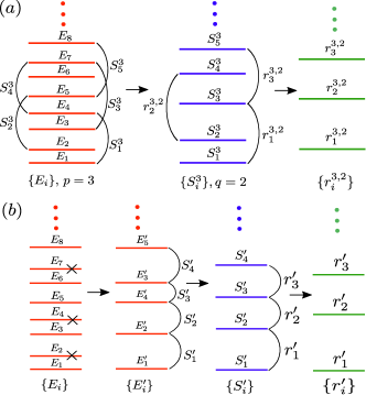
Figure 1: Two new statistics developed in this work. (a) $(p,q)$ level spacing ratios and (b) stochastic level spacing ratios.

The disordered many-body models with short range interaction are obviously totally different from that in RMT, in which all the matrix entries with identical independent distribution are presented. This long range feature can not be captured by the $r$-statistics based on nearest-neighbor level spacings Atas et al. (2013a); Chavda and Kota (2013); Janarek et al. (2018); Oganesyan and Huse (2007). In this work we present two new approaches to characterize the long-distance level spacings in a disordered many-body models. In the first approach, we introduce the $(p,q)$ statistics to measure the level spacing ratios between distant energy levels. Meanwhile, we randomly eliminate some of the energy levels, keeping only $\eta\%$ of them, and then measure the reserved levels using $r$-statistics. Some analytical expressions are obtained for these statistics, which automatically satisfy the inverse relation and duality relation. We find that the results in the disordered many-body models agree well with the predictions from the standard Gaussian orthogonal ensemble (GOE) and unitary ensemble (GUE). These new statistics also satisfy the universal scaling laws during phase transition from the Gaussian ensembles to the Poisson ensemble (PE), with critical disorder strength and its exponent independent of these measurements. Our results shade new insight to the strong energy level interactions and their stability in disordered many-body systems.

Table 1: Validity of the unified distribution for the three ensembles. $\langle r\rangle_{\text{RM}}$ is obtained from Gaussian random matrices with size $N=10^{4}$ averaged over $2\cdot 10^{4}$ realizations, and $\langle r\rangle_{\text{th}}$ is obtained from Eq. 6.

		GOE ($\beta=1$)		GUE ($\beta=2$)		GSE ($\beta=4$)
p	q	$\langle r\rangle_{\text{RM}}$	$\langle r\rangle_{\text{th}}$	$\langle r\rangle_{\text{RM}}$	$\langle r\rangle_{\text{th}}$	$\langle r\rangle_{\text{RM}}$	$\langle r\rangle_{\text{th}}$
1	1	0.5307	0.5359	0.5997	0.6027	0.6744	0.6762
1	2	0.5548	0.5505	0.6266	0.6185	0.7006	0.6919
1	3	0.5606	0.5585	0.6316	0.6271	0.7046	0.7002
1	4	0.5626	0.5635	0.6333	0.6324	0.7059	0.7054
2	1	0.7396	0.7383	0.7870	0.7866	0.8334	0.8340
2	2	0.6744	0.6762	0.7336	0.7335	0.7908	0.7902
2	3	0.6940	0.6919	0.7539	0.7480	0.8090	0.8027
2	4	0.7000	0.7002	0.7589	0.7556	0.8128	0.8092
3	1	0.8202	0.8198	0.8541	0.8540	0.8867	0.8865
3	2	0.7802	0.7811	0.8258	0.8256	0.8665	0.8669
3	3	0.7460	0.7464	0.7970	0.7964	0.8432	0.8429
3	4	0.7618	0.7606	0.8127	0.8087	0.8568	0.8530
4	1	0.8624	0.8624	0.8888	0.8887	0.9139	0.9138
4	2	0.8329	0.8335	0.8685	0.8686	0.8998	0.9000
4	3	0.8132	0.8144	0.8545	0.8544	0.8896	0.8897
4	4	0.7909	0.7902	0.8347	0.8344	0.8736	0.8740
10	3	0.9239	0.9242	0.9412	0.9412	0.9557	0.9557
10	5	0.9157	0.9156	0.9355	0.9356	0.9515	0.9515
10	8	0.9057	0.9054	0.9285	0.9284	0.9462	0.9459
10	10	0.8935	0.8947	0.9184	0.9209	0.9382	0.9419
10	11	0.8997	0.9018	0.9240	0.9264	0.9426	0.9461
10	12	0.9022	0.9055	0.9259	0.9292	0.9438	0.9481

Physical Models and Measurements. We consider the following disordered spin-${1\over 2}$ spin chain Žnidarič et al. (2008); Serbyn et al. (2014a, b); Roy et al. (2018)

$$H=\sum_{i=1}^{L}J(e^{i\theta}S_{i}^{+}S_{i+1}^{-}+\text{h.c.})+J_{z}S_{i}^{z}S_{i+1}^{z}+h_{i}S_{i}^{z},$$ (1)

where $h_{i}$ is a uniform random potential in $[-W,W]$, $S_{i+L}=S_{i}$ from periodic boundary condition and $L$ is the total length of chain. In case $J_{z}=J$, previous inversions have unveiled a critical disorder strength $W_{c}\sim 3-4$ Pal and Huse (2010); Luitz et al. (2015); Serbyn et al. (2015); Luitz et al. (2016). When $W<W_{c}$, it gives an ergodic phase with energy level spacings to be described by GOE ($\theta=0$) or GUE ($\theta\neq 2\pi n/L$, $n\in\mathbb{Z}$ pbc ). In contrast, in the MBL phase ($W>W_{c}$), it follows the Poisson distribution. In the above model, the total spin $S_{\text{tot}}^{z}=\sum_{i}S_{i}^{z}$ is conserved and in the numerical simulation, we will focus on the largest subspace with $S_{\text{tot}}=L/2-[L/2]$. Let us denote the energy levels to be $\{E_{i}\}$ sorted in ascending order, and define the $p$-level spacing as $S_{i}^{p}=E_{i+p}-E_{i}$, then we can define the $(p,q)$ level spacing ratios as

$$r=r_{i}^{p,q}=\frac{\min(S^{p}_{i+q},S^{p}_{i})}{\max(S^{p}_{i+q},S^{p}_{i})},\quad i,p,q=1,2,\cdots.$$ (2)

The picture for this definition is shown in Fig. 1 (a). When $p<q$, there is no overlap between the two $p$-level spacings; while when $p>q$, some overlap between them exists. In the second approach, we randomly eliminate some of the energy levels, keeping only $\eta\%$ of them, which is then measured using the nearest-neighbor $r$-statistics (see Fig. 1 (b)). These two measurements aim to explore the long-distance energy level interactions induced by the random potential, which is a typical feature RMT.

Random Gaussian Ensembles. To further benchmark these results, we consider these measurements in the Gaussian ensembles belonging to GOE, GUE and Gaussian symplectic ensemble (GSE) for $\beta=$ 1, 2, 4, respectively. The joint distribution function (JDF) is Mehta (2004),

$$\rho_{\beta}(E_{1},...,E_{N})=C_{\beta,N}\prod_{i<j}|E_{i}-E_{j}|^{\beta}e^{-\frac{\beta}{2}\sum_{i}E_{i}^{2}}.$$ (3)

To determine the distribution of $r_{i}^{p,q}$, we need to consider the JDF at least with order $N=p+q+1$. In the above equation, we can define $E_{1}=\lambda_{0}$, $E_{i}=\lambda_{0}+\sum_{j=1}^{i-1}\lambda_{j}$ $(i=2,3,\ldots,N)$, then we obtain

$$P_{\beta}(r,p,q)\varpropto\int\prod_{n=0}^{p+q}\text{d}\lambda_{n}\rho_{\beta}(\Lambda_{0}^{0},\ldots,\Lambda_{0}^{p+q})\delta(r-\frac{\Lambda_{1+q}^{p+q}}{\Lambda_{1}^{p}}),$$ (4)

where $\Lambda_{a}^{b}=\sum_{i=a}^{b}\lambda_{i}$. For $p=q=1$ and $N=3$, the distribution $P_{\beta}(r,1,1)$ is studied in Atas et al. (2013a). For $N=4$, we can obtain $P_{\beta}(r,1,2)$ and $P_{\beta}(r,2,1)$, which can also be found in Atas et al. (2013b). For $N>4$, this expression will become formidable. By analysing the solvable cases with $N\leq 4$, we find that the following quadratic function will always be presented in square root,

$$g(r,k)=a_{k}+\text{sgn}(q-p)kr+a_{k}r^{2},$$ (5)

where $k=|p-q|+1$ and $a_{k}=a_{k-1}+k$ with $a_{0}=0$, and $\text{sgn}(x)$ is the sign function with $\text{sgn}(0)=1$. Here $k$ can be regarded as how many energy levels are spaced between two spacings for $p<q$, or the overlap between them for $p>q$. Obviously, $g(k,r)>0$ for any $r$ and $k$. The key observation is that we assert this quadratic function is essential for the distribution function.

For $p\leq q$, we obtain a very accurate approximated distribution $P_{\beta}(r,p,q)$, which is given by

$$P_{\beta}(r,p,q)=C_{\beta}\frac{(r+r^{2})^{\beta_{p}}}{[g(r,k)]^{1+\frac{3}{2}\beta_{p}}},$$ (6)

where $\beta_{p}=\frac{p(p+1)}{2}\beta+p-1$ and $C_{\beta}$ is the normalized constant. This unified distribution for the three ensembles are one important finding in this work. It has a number of interesting features. (I) It automatically satisfies the inverse relation Atas et al. (2013a),

$$P_{\beta}(r,p,q)=P_{\beta}(1/r,p,q)/r^{2},$$ (7)

as required by definition of Eq. 2. (II) When $p=q$, we find $k=1$ and $a_{k}=1$, which will yields duality between GOE and GSE as following,

$$P_{1}(r,2p,2p)=P_{4}(r,p,p),\quad p=1,2,3,\cdots.$$ (8)

It means that the $(2p,2p)$ distribution in GOE is the same as ($p,p$) distribution in GSE. Two examples ($p=1,2$) for this duality can be found in Table 1, and more examples are listed in Ref. ppd . The duality for $p=1$ has been unveiled by Forrester in Forrester (2009) from the exact duality in sense of JDF. Our numerical results may suggest more relations in these ensembles. For instance, we may even find $P_{1}(r,7,7)=P_{2}(r,5,5)$ with $\langle r\rangle_{\text{RM}}=0.8602$ ppd .

For $p>q$, there is an overlap between adjacent $p$-level spacings. We find that the distribution of $r$ can also be given by Eq. 6 with some different $\beta_{p}$, which can be written as $\beta_{p}=ap^{2}+bp+c$ for the same $q$ and $\beta$. The values for $a$, $b$ and $c$ are fitting parameters abc . In Table 1 we present $\langle r\rangle_{\text{th}}$ form Eq. 6 and $\langle r\rangle_{\text{RM}}$ from the Gaussian ensembles, which exhibit excellent agreement between these two descriptions.

Next we discuss the stochastic level spacing ratios $r^{\prime}$ by considering some randomly selected energy levels (see Fig. 1 (b)). We find that the distribution in these three ensembles can still be written as,

$$P_{\beta}(r^{\prime})=C^{\prime}_{\beta}\frac{(r^{\prime}+r^{\prime^{2}})^{\beta^{\prime}}}{(1+tr^{\prime}+r^{\prime^{2}})^{1+\frac{3}{2}\beta^{\prime}}},$$ (9)

where $C^{\prime}_{\beta}$ is a normalized constant and $t$ and $\beta^{\prime}$ are fitted parameters, which depends on $\eta$. This new distribution also satisfies the inversion symmetry in Eq. 7. The numerical results and their best fitting can be found in Fig. 2 (a) - (d), and their corresponding $\beta^{\prime}$ and $t$ are presented in Fig. 2 (e) - (f). When $\eta\rightarrow 0$, we find $\beta^{\prime}\rightarrow 0$ and $t\rightarrow 2$, which realizes a transition from Gaussian ensembles to Poisson distribution,

$$P_{\text{PE}}(r^{\prime})={2\over(1+r^{\prime})^{2}}.$$ (10)

This is expected since the stochastic energy levels in the small $\eta$ limit has completely erased the correlation between them, which is the essential assumption during the derivation of Poisson distribution Mehta (2004). With this method we may realize some distributions in Laguerre $\beta$-ensembles Dumitriu and Edelman (2002, 2006), which exhibit some dualities in JDP Forrester (2009). These results also demonstrate the excellent predictability of Eqs. 6 and 9.

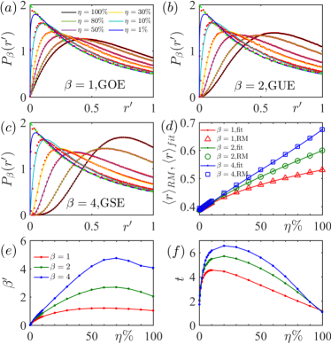
Figure 2: (a) - (c) Distribution of the stochastic level spacing ratios for the three Gaussian ensembles. Red dots are the numerical results from Gaussian matrices with size $N=10^{4}$ averaged over $2\cdot 10^{4}$ realizations, and the solid lines are corresponding best fit with Eq. 9. The green dashed lines are given by Eq. 10. (d) The average value of $r^{\prime}$, where $\langle r^{\prime}\rangle_{\text{RM}}$ (open symbols) are determined numerically from Gaussian ensembles and $\langle r^{\prime}\rangle_{\text{fit}}$ (solid lines) are calculated from Eq. 9. (e) - (f) fitted parameters of $\beta^{\prime}$ and $t$ as a function of $\eta$.

Poisson Ensemble. Now we consider the $(p,q)$ statistics for Poisson random variables $\{E_{i}\}$. Using the previous method, we find

$$P_{\text{PE}}(r,p,q)=\int_{0}^{\infty}\prod_{i=0}^{p+q}\text{d}\lambda_{i}e^{-\Lambda_{0}^{p+q}}\delta(r-\frac{\Lambda_{1+q}^{p+q}}{\Lambda_{1}^{p}}).$$ (11)

For $p\leq q$, the distribution $P_{\text{PE}}(r,p,q)$ is given by

$$P_{\text{PE}}(r,p,q)=\frac{1}{C_{p}}\frac{r^{p-1}}{(1+r)^{2p}}.$$ (12)

When $p=1$, this function yields Eq. 10. Then we obtain $\langle r\rangle_{\text{PE}}=_{2}F_{1}(2p,1+p;2+p;-1)\Gamma(1+p)p/_{2}F_{1}(p,2p;1+p;-1)\Gamma(2+p)$, where ${}_{2}F_{1}$ is the hypergeometric series Gasper and Rahman (2004); Bailey (1928). The values of this mean value for $p=1$ to $6$ can be found in Ref. ppd . This distribution also satisfies the inverse relation in Eq. 7.

For $p>q$, we denote $x=\Lambda_{q+1}^{p}$, then Eq. 11 can be rewritten as

$$P_{\text{PE}}(r,p,q)= \int_{0}^{\infty}\text{d}x\prod_{i=1}^{q}\text{d}\lambda_{i}\prod_{j=p+1}^{p+q}\text{d}\lambda_{j}e^{-\Lambda_{1}^{q}-\Lambda_{p+1}^{p+q}}$$

$$\cdot\frac{x^{p-q-1}}{(p-q-1)!e^{-x}}\delta(r-\frac{x+\Lambda_{p+1}^{p+q}}{\Lambda_{1}^{q}+x}),$$ (13)

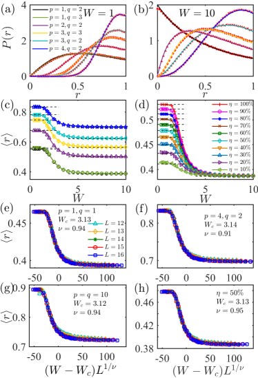
Figure 3: GOE with $\theta=0$. (a) In ergodic phase ($W=1$) and (b) in MBL phase ($W=10$), where symbols are data averaged over 4000 realizations in a chain with $L=14$, and dashed lines are these given by Eqs. 6, 11 and 14. (c) The $(p,q)$ statistics as a function of $W$. The symbols are the same as the six cases studied in (a). (d) The stochastic statistics for different reserved rate $\eta$. In (c) and (d) the horizontal dashed lines are given by $\langle r\rangle_{\text{th}}$, $\langle r^{\prime}\rangle_{\text{fit}}$ or $\langle r\rangle_{\text{PE}}$. (e) - (h) The data collapse used to extract the critical disorder strength $W_{c}$ and exponent $\nu$ for the different measurements. These data are averaged over 7000, 5000, 4000, 1000 and 300 realizations for $L=12-16$, respectively.

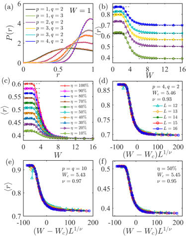
Figure 4: GUE with $\theta=\pi/28$. (a) In ergodic phase ($W=1$). (b) - (c) The variation of $\langle r\rangle$ for different $(p,q)$ and $\eta$, respectively. (e) - (f) Methods to extract $W_{c}$ and $\nu$. The other legend descriptions are the same as that in Fig. 3.

For $0<r<1$, we find $P_{\text{PE}}(r,p,q)$ can be expressed as

$$P_{\text{PE}}(r,p,q)=\frac{2r^{p-1}}{(1+r)^{2q}}\sum_{m=0}^{2q-1}r^{m}w_{m},$$ (14)

where $w_{m}$ is given by

$$w_{m}=(-1)^{n}\mathcal{Y}_{q,n+1}f_{m-n,q-1}^{p}f_{-q,m-n-(q+1)}^{p},$$ (15)

where $n=[m/2]$ and $\mathcal{Y}_{i,j}$ is a number of the $i$-th row and $j$-th column of the Yang Hui’s triangle Yadav and Mohan (2011), and $f_{a,b}^{p}=\Gamma(p+b+1)/\Gamma(p+a)$. For $q=1$, Eq. 14 will yields,

$$P_{\text{PE}}(r,p,1)=\left\{\begin{aligned} &{r^{p-1}(p+(p-1)r)\over(1+r)^{2}},\quad 0<r<1\\ &\frac{p-1+pr}{r^{p}(1+r)^{2}},\quad r>1\end{aligned}\right.$$ (16)

which was also shown in Atas et al. (2013b). These expressions also satisfy Eq. 7.

Many-body systems and MBL. Finally we use the above results to understand the distribution in Eq. 1. In GOE (Fig. 3), we consider $J=1/2$, $J_{z}=1$ and $\theta=0$ and in GUE (Fig. 4), we consider $J=J_{z}=1$ and $\theta=\pi/28$. We employ the exact diagonalization (ED) method to study these two new statistics in a finite system and compare them with the analytical expressions obtained in the previous paragraphs. We normalize the eigenvalues using $\varepsilon=(E-E_{\min})/(E_{\max}-E_{\min})$, where $E_{\min}$ $(E_{\max})$ are the energies of the ground state (highest excited state) of the system. For different $\varepsilon$, there is a different $W_{c}$, indicating of many-body mobility edges Mondragon-Shem et al. (2015); Luitz et al. (2015); Laumann et al. (2014); Baygan et al. (2015). In this paper, we mainly discuss the case of $\varepsilon=0.5\pm 0.15$ in the middle of the spectra. For $(p,q)$ level spacing ratios, the results are shown in Fig. 3 (a) - (b) and Fig. 4 (a), with $W=1$ to the physics in GOE or GUE, and $W=10$ to that in PE. In Fig. 3 (c) - (d) and Fig. 4 (b) - (c), we give the variation of $\langle r\rangle$ with $W$ for different $(p,q)$ and $\eta$. In Fig. 3 (e) - (h) and Fig. 4 (d) - (f), we show our new statistics also satisfy the scaling laws. For $\theta=0$ (GOE), we obtain $W_{c}\approx 3.13\pm 0.02$ and $\nu\approx 0.94\pm 0.03$, in consistent with Ref. Luitz et al. (2015) with $W_{c}\approx 3.72$ and $\nu\approx 0.91\pm 0.03$ Wcd . For $\theta=\pi/28$ (GUE), we obtain $W_{c}\approx 5.44\pm 0.03$ and $\nu\approx 0.95\pm 0.04$. All these results shown that the critical disorder strength $W_{c}$ and the exponent $\nu$ do not change significantly in these two measurements with different $(p,q)$ and $\eta$, demonstrating their universality in Gaussian ensembles.

Conclusion. We introduce two new approaches to characterize the long-distance energy level interactions in the disordered many-body systems. Some analytical distributions with high accuracy are obtained by benchmarking these results against the RMT. These expressions also automatically satisfy the inverse relation and duality relation. These new statistics also yield some universal scaling laws, in which the critical exponent and critical disorder strength are almost independent of the choice of the two different statistics. Our results indicate that although the physical models are made by short-range interaction, their energy levels are long-range correlated. These features may also be revealed from the entanglement entropy Ponte et al. (2015); Vasseur et al. (2015); Bera et al. (2015); Luitz et al. (2016), inverse participation ratios Serbyn et al. (2013); Iyer et al. (2013); Torres-Herrera and Santos (2015) and spin imbalance Luitz et al. (2016); Zhang et al. (2016) using only a fraction of spectra. Our results demonstrate the robustness of MBL phases and their universal features.

Acknowledgements. We thank Prof. Dang-Zheng Liu for valuable discussion. This work is supported by the National Youth Thousand Talents Program (No. KJ2030000001), the USTC start-up funding (No. KY2030000053), the NSFC (No. 11774328) and the National Key Research and Development Program of China (No. 2016YFA0301700).

References

- Anderson (1958) Philip W Anderson, “Absence of diffusion in certain random lattices,” Phys. Rev. 109, 1492 (1958).
- Abrahams (2010) Elihu Abrahams, 50 years of Anderson Localization (world scientific, 2010).
- Abrahams et al. (1979) Elihu Abrahams, PW Anderson, DC Licciardello, and TV Ramakrishnan, “Scaling theory of localization: Absence of quantum diffusion in two dimensions,” Phys. Rev. Lett. 42, 673 (1979).
- Wigner (1951) Eugene P Wigner, “On the statistical distribution of the widths and spacings of nuclear resonance levels,” in Math. Proc. Cambridge Philos. Soc., Vol. 47 (Cambridge University Press, 1951) pp. 790–798.
- Mehta (2004) Madan Lal Mehta, Random matrices, Vol. 142 (Elsevier, 2004).
- Wigner (1993a) Eugene P Wigner, “Characteristic vectors of bordered matrices with infinite dimensions i,” in The Collected Works of Eugene Paul Wigner (Springer, 1993) pp. 524–540.
- Wigner (1993b) Eugene P Wigner, “Characteristic vectors of bordered matrices with infinite dimensions ii,” in The Collected Works of Eugene Paul Wigner (Springer, 1993) pp. 541–545.
- Dyson (1962) Freeman J Dyson, “Statistical theory of the energy levels of complex systems. i,” J. Math. Phys. 3, 140–156 (1962).
- Altshuler and Shklovskii (1986) BL Altshuler and BI Shklovskii, “Repulsion of energy levels and conductivity of small metal samples,” Sov. Phys. JETP 64, 127–135 (1986).
- Beenakker (2015) CWJ Beenakker, “Random-matrix theory of majorana fermions and topological superconductors,” Rev. Mod. Phys. 87, 1037 (2015).
- Pal and Huse (2010) Arijeet Pal and David A Huse, “Many-body localization phase transition,” Phys. Rev. B 82, 174411 (2010).
- Žnidarič et al. (2008) Marko Žnidarič, Tomaž Prosen, and Peter Prelovšek, “Many-body localization in the heisenberg xxz magnet in a random field,” Phys. Rev. B 77, 064426 (2008).
- Kjäll et al. (2014) Jonas A Kjäll, Jens H Bardarson, and Frank Pollmann, “Many-body localization in a disordered quantum ising chain,” Phys. Rev. Lett. 113, 107204 (2014).
- Altman (2018) Ehud Altman, “Many-body localization and quantum thermalization,” Nature Phys. 14, 979 (2018).
- Oganesyan and Huse (2007) Vadim Oganesyan and David A Huse, “Localization of interacting fermions at high temperature,” Phys. Rev. B 75, 155111 (2007).
- Vosk et al. (2015) Ronen Vosk, David A Huse, and Ehud Altman, “Theory of the many-body localization transition in one-dimensional systems,” Phys. Rev. X 5, 031032 (2015).
- Luitz et al. (2015) David J Luitz, Nicolas Laflorencie, and Fabien Alet, “Many-body localization edge in the random-field heisenberg chain,” Phys. Rev. B 91, 081103 (2015).
- Serbyn and Moore (2016) Maksym Serbyn and Joel E Moore, “Spectral statistics across the many-body localization transition,” Phys. Rev. B 93, 041424 (2016).
- Zhang and Yao (2018) Shi-Xin Zhang and Hong Yao, “Universal properties of many-body localization transitions in quasiperiodic systems,” Phys. Rev. Lett. 121, 206601 (2018).
- Tasaki (1998) Hal Tasaki, “From quantum dynamics to the canonical distribution: general picture and a rigorous example,” Phys. Rev. Lett. 80, 1373 (1998).
- Rigol et al. (2008) Marcos Rigol, Vanja Dunjko, and Maxim Olshanii, “Thermalization and its mechanism for generic isolated quantum systems,” Nature 452, 854 (2008).
- Vitagliano et al. (2010) Giuseppe Vitagliano, Arnau Riera, and José Ignacio Latorre, “Volume-law scaling for the entanglement entropy in spin-1/2 chains,” New J. Phys. 12, 113049 (2010).
- Khemani et al. (2017) Vedika Khemani, DN Sheng, and David A Huse, “Two universality classes for the many-body localization transition,” Phys. Rev. Lett. 119, 075702 (2017).
- Canovi et al. (2011) Elena Canovi, Davide Rossini, Rosario Fazio, Giuseppe E Santoro, and Alessandro Silva, “Quantum quenches, thermalization, and many-body localization,” Phys. Rev. B 83, 094431 (2011).
- Ponte et al. (2015) Pedro Ponte, Z Papić, François Huveneers, and Dmitry A Abanin, “Many-body localization in periodically driven systems,” Phys. Rev. Lett. 114, 140401 (2015).
- Devakul and Singh (2015) Trithep Devakul and Rajiv RP Singh, “Early breakdown of area-law entanglement at the many-body delocalization transition,” Phys. Rev. Lett. 115, 187201 (2015).
- Huse et al. (2014) David A Huse, Rahul Nandkishore, and Vadim Oganesyan, “Phenomenology of fully many-body-localized systems,” Phys. Rev. B 90, 174202 (2014).
- Geraedts et al. (2016) Scott D Geraedts, Rahul Nandkishore, and Nicolas Regnault, “Many-body localization and thermalization: Insights from the entanglement spectrum,” Phys. Rev. B 93, 174202 (2016).
- Nandkishore and Huse (2015) Rahul Nandkishore and David A Huse, “Many-body localization and thermalization in quantum statistical mechanics,” Annu. Rev. Condens. Matter Phys. 6, 15–38 (2015).
- Alet and Laflorencie (2018) Fabien Alet and Nicolas Laflorencie, “Many-body localization: an introduction and selected topics,” Comp. Rendus Phys. (2018).
- Abanin et al. (2018) Dmitry A Abanin, Ehud Altman, Immanuel Bloch, and Maksym Serbyn, “Ergodicity, entanglement and many-body localization,” arXiv preprint arXiv:1804.11065 (2018).
- Atas et al. (2013a) Y. Y Atas, E Bogomolny, O Giraud, and G Roux, “Distribution of the ratio of consecutive level spacings in random matrix ensembles,” Phys. Rev. Lett. 110, 084101 (2013a).
- Chavda and Kota (2013) ND Chavda and VKB Kota, “Probability distribution of the ratio of consecutive level spacings in interacting particle systems,” Phys. Rev. A 377, 3009–3015 (2013).
- Janarek et al. (2018) Jakub Janarek, Dominique Delande, and Jakub Zakrzewski, “Discrete disorder models for many-body localization,” Phys. Rev. B 97, 155133 (2018).
- Serbyn et al. (2014a) Maksym Serbyn, Z Papić, and Dmitry A Abanin, “Quantum quenches in the many-body localized phase,” Phys. Rev. B 90, 174302 (2014a).
- Serbyn et al. (2014b) M Serbyn, Michael Knap, Sarang Gopalakrishnan, Z Papić, Norman Ying Yao, CR Laumann, DA Abanin, Mikhail D Lukin, and Eugene A Demler, “Interferometric probes of many-body localization,” Phys. Rev. Lett. 113, 147204 (2014b).
- Roy et al. (2018) Sthitadhi Roy, Achilleas Lazarides, Markus Heyl, and Roderich Moessner, “Dynamical potentials for nonequilibrium quantum many-body phases,” Phys. Rev. B 97, 205143 (2018).
- Serbyn et al. (2015) Maksym Serbyn, Z Papić, and Dmitry A Abanin, “Criterion for many-body localization-delocalization phase transition,” Phys. Rev. X 5, 041047 (2015).
- Luitz et al. (2016) David J Luitz, Nicolas Laflorencie, and Fabien Alet, “Extended slow dynamical regime close to the many-body localization transition,” Phys. Rev. B 93, 060201 (2016).
- (40) We consider periodic boundary condition, in which when , the phases between the neighboring sites can be gauged out by defining , in which we find . In a system with open boundary condition, this phase will not yields new different observations in the statistics of energy levels.
- Atas et al. (2013b) Y. Y Atas, E Bogomolny, O Giraud, P Vivo, and E Vivo, “Joint probability densities of level spacing ratios in random matrices,” J. Phys. A: Math. Theor. 46, 355204 (2013b).
- (42) We find that in both GOE and GSE are 0.8434, 0.8739, 0.8940, 0.9083 for 6, 8, 10, 12, respectively. We also find this value is 0.8602 in GOE ensemble for , while in GUE, it is 0.8605 for . The mean value are 0.3863, 0.500, 0.5625, 0.6042, 0.6348, 0.6586 for to , respectively.
- Forrester (2009) Peter J Forrester, “A random matrix decimation procedure relating = 2/(r+ 1) to = 2 (r+ 1),” Commun. Math. Phys. 285, 653–672 (2009).
- (44) for , 2, 4 are: , , for ; , , for ; , , for ; , , for ; , , for .
- Dumitriu and Edelman (2002) Ioana Dumitriu and Alan Edelman, “Matrix models for beta ensembles,” J. Math. Phys. 43, 5830–5847 (2002).
- Dumitriu and Edelman (2006) Ioana Dumitriu and Alan Edelman, “Global spectrum fluctuations for the -hermite and -laguerre ensembles via matrix models,” J. Math. Phys. 47, 063302 (2006).
- Gasper and Rahman (2004) George Gasper and Mizan Rahman, Basic hypergeometric series, Vol. 96 (Cambridge university press, 2004).
- Bailey (1928) Wilfrid Norman Bailey, “Products of generalized hypergeometric series,” Proc. London Math. Soc. 2, 242–254 (1928).
- Yadav and Mohan (2011) Bhuri Singh Yadav and Man Mohan, Ancient Indian leaps into mathematics (Springer, 2011).
- Mondragon-Shem et al. (2015) Ian Mondragon-Shem, Arijeet Pal, Taylor L Hughes, and Chris R Laumann, “Many-body mobility edge due to symmetry-constrained dynamics and strong interactions,” Phys. Rev. B 92, 064203 (2015).
- Laumann et al. (2014) Christopher R Laumann, A Pal, and A Scardicchio, “Many-body mobility edge in a mean-field quantum spin glass,” Phys. Rev. Lett. 113, 200405 (2014).
- Baygan et al. (2015) Elliott Baygan, SP Lim, and DN Sheng, “Many-body localization and mobility edge in a disordered spin-1 2 heisenberg ladder,” Phys. Rev. B 92, 195153 (2015).
- (53) In Ref. Luitz et al. (2015), is obtained using , while in this work, is used.
- Vasseur et al. (2015) R Vasseur, SA Parameswaran, and JE Moore, “Quantum revivals and many-body localization,” Phys. Rev. B 91, 140202 (2015).
- Bera et al. (2015) Soumya Bera, Henning Schomerus, Fabian Heidrich-Meisner, and Jens H Bardarson, “Many-body localization characterized from a one-particle perspective,” Phys. Rev. Lett. 115, 046603 (2015).
- Serbyn et al. (2013) Maksym Serbyn, Z Papić, and Dmitry A Abanin, “Local conservation laws and the structure of the many-body localized states,” Phys. Rev. Lett. 111, 127201 (2013).
- Iyer et al. (2013) Shankar Iyer, Vadim Oganesyan, Gil Refael, and David A Huse, “Many-body localization in a quasiperiodic system,” Phys. Rev. B 87, 134202 (2013).
- Torres-Herrera and Santos (2015) E. J Torres-Herrera and Lea F Santos, “Dynamics at the many-body localization transition,” Phys. Rev. B 92, 014208 (2015).
- Zhang et al. (2016) Liangsheng Zhang, Vedika Khemani, and David A Huse, “A floquet model for the many-body localization transition,” Phys. Rev. B 94, 224202 (2016).