Phenomenology of an extended IDM with loop-generated fermion mass hierarchies

Abstract

We perform a comprehensive analysis of the most distinctive and important phenomenological implications of the recently proposed mechanism of sequential loop generation of strong hierarchies in the Standard Model (SM) fermion mass spectra. This mechanism is consistently realized at the level of renormalizable interactions in an extended variant of the Inert Higgs Doublet model, possessing the additional $Z_{2}^{(1)}\times Z_{2}^{(2)}$ discrete and $U_{1X}$ gauge family symmetries, while the matter sectors of the SM are extended by means of $SU_{2L}$-singlet scalars, heavy vector-like leptons and quarks, as well as right-handed neutrinos. We thoroughly analyze the most stringent constraints on the model parameter space, coming from the $Z^{\prime}$ collider searches, related to the anomaly in lepton universality, and the muon anomalous magnetic moment, as well as provide benchmark points for further tests of the model and discuss possible “standard candle” signatures relevant for future explorations.

I Introduction

The hypothetical extensions of the Standard Model (SM) that accommodate a dynamical explanation of the mass and mixing hierarchies in the quark, lepton and neutrino sectors, are typically expected to contain many new interactions and states at high scales of the theory. In particular, additional scalar fields are required to break the high-scale (e.g. discrete or continuous family) symmetries, causing the formation of specific patterns in the fermion mass spectra across generations. The additional inert sectors, such as heavy right-handed neutrinos, are mandatory for see-saw type mechanisms of neutrino mass generation, and play a supplemental but important cosmological role in leptogenesis and also as candidates for DM. In practice, there are no strong constraints on how many additional heavy scalar singlet and vector-like fermion states could be added to the SM at the fundamental level, as they typically produce vanishing direct signatures in collider measurements, but may have indirect (e.g. via radiative corrections) signatures imprinted into the patterns of SM couplings and mass parameters.

In general, additional states are required to explain specific patterns in the SM fermion spectra. For example, to address only the quark sector and to explain the Cabbibo-like structure of the quark mixing simultaneously with the hierarchies in the quark mass spectrum, the addition of a gauged $U_{1X}$ or discrete family symmetry and few extra scalar fields seems to be enough (see Refs. Campos:2014zaa ; Hernandez:2015hrt ; Hernandez:2015dga ; Arbelaez:2016mhg ; Mantilla:2016lui ; CarcamoHernandez:2016pdu ; Bernal:2017xat ; CarcamoHernandez:2017cwi ; Mantilla:2017ijh ; Abbas:2017vws ; Dev:2018pjn ; CarcamoHernandez:2018hst ; Abbas:2018lga ; CarcamoHernandez:2019pmy ; CarcamoHernandez:2019vih ; CarcamoHernandez:2019cbd ). Such models, although not necessarily excluded, may generically suffer from large Flavor-Changing Neutral Currents (FCNCs) and from non-observability of Higgs partners in the few-hundreds GeV mass range. In order to explain the lepton mass hierarchy together with the highly decoupled neutrino mass spectrum, even more additional inputs are required on top of the SM. Due to a large number of states, such theories quickly become cumbersome to deal with and to verify phenomenologically. Therefore, the search for a particular model capable of explaining all the fermion mass and mixing hierarchies in a dynamical and fully renormalizable way, while still having it simple enough for a straightforward phenomenological verification, becomes a challenging and demanding, but very important task for the model-building community.

In addition, models having an extended scalar and (or) fermion sector are motivated by the search of a theoretical explanation for the Lepton Universality Violation (LUV) recently observed by the LHCb experiments. A concise review of New Physics models aimed at explaining the LUV and their possible connection to DM is provided in Ref. Vicente:2018xbv . Some theoretical explanations for the LUV are discussed in Refs. Crivellin:2015era ; Crivellin:2015lwa ; King:2018fcg ; Bonilla:2017lsq ; Barbieri:2017tuq ; King:2017anf ; Romao:2017qnu ; Antusch:2017tud ; Ko:2017quv ; Ko:2017yrd ; Chen:2017hir ; Assad:2017iib ; Angelescu:2018tyl ; DiLuzio:2018zxy ; Guadagnoli:2018ojc ; Fornal:2018dqn ; Aydemir:2018cbb ; Faber:2018qon ; Barman:2018jhz ; Heeck:2018ntp ; Grinstein:2018fgb ; Falkowski:2018dsl ; CarcamoHernandez:2018aon ; deMedeirosVarzielas:2018bcy ; Rocha-Moran:2018jzu ; Hu:2018veh ; Carena:2018cow ; Babu:2018vrl ; Allanach:2018lvl .

In Ref. CarcamoHernandez:2019cbd we have proposed such a possible candidate theory, capable of generating the SM fermion mass and mixing hierarchies via a sequential loop suppression mechanism, in terms of model parameters with no intrinsically imposed hierarchies between them. In this framework the only fermion that acquires its mass at tree level is the heavy top quark. Moderate and light quark masses are generated essentially at one- or two-loop level, respectively, while light active neutrinos become massive only via three-loop radiative seesaw mechanisms triggered after the electroweak symmetry breaking. We have found specific conditions on the minimal symmetry and particle content for a theory where this mechanism can be realized without adding the non-renormalizable (higher-dimensional) Yukawa operators or soft family-breaking mass terms. While such a construction is supposedly not unique, its minimality is manifest as every field plays a relevant role for producing the observed patterns in quark, lepton and neutrino sectors of the SM, with a required degree of suppression between the corresponding SM parameters.

II Review of the extended IDM model

With the aim of generating the hierarchy of SM charged fermion masses via the sequential loop suppression mechanism, proposed for the first time in Ref. CarcamoHernandez:2016pdu , we consider an extension of the inert two-Higgs doublet model (ITHDM), where the SM gauge symmetry is supplemented by an exactly preserved $Z_{2}^{(2)}$ and spontaneously broken $Z_{2}^{(1)}$ discrete groups, and by an $U_{1X}$ gauge symmetry. The scalar sector of the ITHDM is extended to include seven electrically neutral fields, i.e., $\sigma_{j}$ ($j=1,2,3$), $\rho_{k}$ ($k=1,2,3$), $\eta$ and five electrically charged $\varphi_{k}^{+}$ ($k=1,2,3,4,5$) $SU_{2L}$ scalar singlets. The fermion sector of the SM includes additionally six SM gauge-singlet charged leptons $E_{jL}$ and $E_{jR}$ ($j=1,2,3$), four right handed neutrinos $\nu_{jR}$  ($j=1,2,3$), $\Omega_{R}$ and twelve $SU_{2L}$ singlet heavy quarks $T_{L}$, $T_{R}$, $\widetilde{T}_{L}$,$\ \widetilde{T}_{R}$, $B_{kL}$, $B_{kR}$ ($k=1,2,3,4$). It is assumed that the heavy exotic $T$, $\widetilde{T}$ and $B_{k}$ quarks have electric charges equal to $\frac{2}{3}$ and $-\frac{1}{3}$, respectively. The scalar, quark and lepton assignments under the $SU_{3c}\times SU_{2L}\times U_{1Y}\times U_{1X}\times Z_{2}^{(1)}\times Z_{2}^{(2)}$ symmetry are shown in Tables 1, 2 and 3, respectively. It was shown in Ref. CarcamoHernandez:2016pdu that with this field content and the corresponding assignments the gauge anomaly cancellation conditions are satisfied in our model.

Field	$\phi_{1}$	$\phi_{2}$	$\sigma_{1}$	$\sigma_{2}$	$\sigma_{3}$	$\rho_{1}$	$\rho_{2}$	$\rho_{3}$	$\eta$	$\varphi_{1}^{+}$	$\varphi_{2}^{+}$	$\varphi_{3}^{+}$	$\varphi_{4}^{+}$	$\varphi_{5}^{+}$
$SU_{3c}$	$\mathbf{1}$	$\mathbf{1}$	$\mathbf{1}$	$\mathbf{1}$	$\mathbf{1}$	$\mathbf{1}$	$\mathbf{1}$	$\mathbf{1}$	$\mathbf{1}$	$\mathbf{1}$	$\mathbf{1}$	$\mathbf{1}$	$\mathbf{1}$	$\mathbf{1}$
$SU_{2L}$	$\mathbf{2}$	$\mathbf{2}$	$\mathbf{1}$	$\mathbf{1}$	$\mathbf{1}$	$\mathbf{1}$	$\mathbf{1}$	$\mathbf{1}$	$\mathbf{1}$	$\mathbf{1}$	$\mathbf{1}$	$\mathbf{1}$	$\mathbf{1}$	$\mathbf{1}$
$U_{1Y}$	$\frac{1}{2}$	$\frac{1}{2}$	$0$	$0$	$0$	$0$	$0$	$0$	$0$	$1$	$1$	$1$	$1$	$1$
$U_{1X}$	$1$	$2$	$-1$	$-1$	$-2$	$0$	$0$	$0$	$1$	$5$	$2$	$3$	$2$	$3$
$Z_{2}^{(1)}$	$1$	$1$	$1$	$1$	$-1$	$1$	$-1$	$-1$	$-1$	$-1$	$1$	$1$	$-1$	$-1$
$Z_{2}^{(2)}$	$1$	$-1$	$1$	$-1$	$-1$	$-1$	$-1$	$1$	$-1$	$1$	$1$	$-1$	$1$	$1$

Table 1: Scalars assignments under the $SU_{3c}\times SU_{2L}\times U_{1Y}\times U_{1X}\times Z_{2}^{(1)}\times Z_{2}^{(2)}$ symmetry.

Field	$q_{1L}$	$q_{2L}$	$q_{3L}$	$u_{1R}$	$u_{2R}$	$u_{3R}$	$d_{1R}$	$d_{2R}$	$d_{3R}$	$T_{L}$	$T_{R}$	$\widetilde{T}_{L}$	$\widetilde{T}_{R}$	$B_{1L}$	$B_{1R}$	$B_{2L}$	$B_{2R}$	$B_{3L}$	$B_{3R}$	$B_{4L}$	$B_{4R}$
$SU_{3c}$	$\mathbf{3}$	$\mathbf{3}$	$\mathbf{3}$	$\mathbf{3}$	$\mathbf{3}$	$\mathbf{3}$	$\mathbf{3}$	$\mathbf{3}$	$\mathbf{3}$	$\mathbf{3}$	$\mathbf{3}$	$\mathbf{3}$	$\mathbf{3}$	$\mathbf{3}$	$\mathbf{3}$	$\mathbf{3}$	$\mathbf{3}$	$\mathbf{3}$	$\mathbf{3}$	$\mathbf{3}$	$\mathbf{3}$
$SU_{2L}$	$\mathbf{2}$	$\mathbf{2}$	$\mathbf{2}$	$\mathbf{1}$	$\mathbf{1}$	$\mathbf{1}$	$\mathbf{1}$	$\mathbf{1}$	$\mathbf{1}$	$\mathbf{1}$	$\mathbf{1}$	$\mathbf{1}$	$\mathbf{1}$	$\mathbf{1}$	$\mathbf{1}$	$\mathbf{1}$	$\mathbf{1}$	$\mathbf{1}$	$\mathbf{1}$	$\mathbf{1}$	$\mathbf{1}$
$U_{1Y}$	$\frac{1}{6}$	$\frac{1}{6}$	$\frac{1}{6}$	$\frac{2}{3}$	$\frac{2}{3}$	$\frac{2}{3}$	$-\frac{1}{3}$	$-\frac{1}{3}$	$-\frac{1}{3}$	$\frac{2}{3}$	$\frac{2}{3}$	$\frac{2}{3}$	$\frac{2}{3}$	$-\frac{1}{3}$	$-\frac{1}{3}$	$-\frac{1}{3}$	$-\frac{1}{3}$	$-\frac{1}{3}$	$-\frac{1}{3}$	$-\frac{1}{3}$	$-\frac{1}{3}$
$U_{1X}$	$0$	$0$	$1$	$2$	$2$	$2$	$-1$	$-1$	$-1$	$1$	$2$	$1$	$1$	$0$	$-1$	$0$	$-1$	$-2$	$-2$	$-3$	$-3$
$Z_{2}^{(1)}$	$1$	$1$	$1$	$-1$	$-1$	$1$	$-1$	$-1$	$-1$	$1$	$1$	$-1$	$-1$	$1$	$1$	$1$	$1$	$1$	$1$	$1$	$1$
$Z_{2}^{(2)}$	$-1$	$-1$	$-1$	$-1$	$-1$	$-1$	$-1$	$-1$	$-1$	$1$	$1$	$-1$	$-1$	$1$	$1$	$1$	$1$	$1$	$1$	$-1$	$-1$

Table 2: Quark assignments under the $SU_{3c}\times SU_{2L}\times U_{1Y}\times U_{1X}\times Z_{2}^{(1)}\times Z_{2}^{(2)}$ symmetry.

Field	$l_{1L}$	$l_{2L}$	$l_{3L}$	$l_{1R}$	$l_{2R}$	$l_{3R}$	$E_{1L}$	$E_{1R}$	$E_{2L}$	$E_{2R}$	$E_{3L}$	$E_{3R}$	$\nu_{1R}$	$\nu_{2R}$	$\nu_{3R}$	$\Omega_{1R}$	$\Omega_{2R}$	$\Psi_{R}$
$SU_{3c}$	$\mathbf{1}$	$\mathbf{1}$	$\mathbf{1}$	$\mathbf{1}$	$\mathbf{1}$	$\mathbf{1}$	$\mathbf{1}$	$\mathbf{1}$	$\mathbf{1}$	$\mathbf{1}$	$\mathbf{1}$	$\mathbf{1}$	$\mathbf{1}$	$\mathbf{1}$	$\mathbf{1}$	$\mathbf{1}$	$\mathbf{1}$	$\mathbf{1}$
$SU_{2L}$	$\mathbf{2}$	$\mathbf{2}$	$\mathbf{2}$	$\mathbf{1}$	$\mathbf{1}$	$\mathbf{1}$	$\mathbf{1}$	$\mathbf{1}$	$\mathbf{1}$	$\mathbf{1}$	$\mathbf{1}$	$\mathbf{1}$	$\mathbf{1}$	$\mathbf{1}$	$\mathbf{1}$	$\mathbf{1}$	$\mathbf{1}$	$\mathbf{1}$
$U_{1Y}$	$-\frac{1}{2}$	$-\frac{1}{2}$	$-\frac{1}{2}$	$-1$	$-1$	$-1$	$-1$	$-1$	$-1$	$-1$	$-1$	$-1$	$0$	$0$	$0$	$0$	$0$	$0$
$U_{1X}$	$0$	$-3$	$0$	$-3$	$-6$	$-3$	$-3$	$-2$	$-6$	$-5$	$-3$	$-2$	$2$	$-1$	$2$	$-1$	$1$	$0$
$Z_{2}^{(1)}$	$1$	$-1$	$1$	$1$	$-1$	$1$	$-1$	$-1$	$-1$	$-1$	$1$	$1$	$1$	$-1$	$1$	$-1$	$-1$	$1$
$Z_{2}^{(2)}$	$-1$	$-1$	$-1$	$-1$	$-1$	$-1$	$1$	$1$	$1$	$1$	$1$	$1$	$1$	$1$	$1$	$-1$	$1$	$1$

Table 3: Lepton charge assignments under the $SU_{3c}\times SU_{2L}\times U_{1Y}\times U_{1X}\times Z_{2}^{(1)}\times Z_{2}^{(2)}$ symmetry.

Let us note that the SM Higgs doublet, i.e., $\phi_{1}$, as well as the SM scalar singlets $\sigma_{1}$ and $\rho_{3}$ are the only scalar fields neutral under the preserved $Z_{2}^{(2)}$ discrete symmetry. Since the $Z_{2}^{(2)}$ symmetry remains unbroken, the SM Higgs doublet $\phi_{1}$ and the SM scalar singlets $\sigma_{1}$ and $\rho_{3}$ are the only scalar fields which acquire nonvanishing vacuum expectation values. The SM scalar singlet $\sigma_{1}$ is required to spontaneously break the $U_{1X}$ local symmetry, whereas the scalar singlet $\rho_{3}$ spontaneously breaks the $Z_{2}^{(1)}$ discrete symmetry, due to its nontrivial $Z_{2}^{(1)}$ charge.

In the following we provide a brief justification for introducing different particles in our model. It is worth mentioning that the set of $SU_{2L}$-singlet heavy quarks $T_{L}$, $T_{R}$, $B_{iL}$, $B_{iR}$ ($i=1,2,3$) represents the minimal amount of exotic quark degrees of freedom needed to implement the one-loop radiative seesaw mechanism that gives rise to the charm, bottom and strange quark masses. In addition, to implement this one-loop radiative seesaw mechanism, one needs the extra $\phi_{2}$ scalar doublet, the gauge singlet scalars $\rho_{2}$, $\rho_{3}$ and $\eta$, charged under the preserved $Z_{2}^{(2)}$ symmetry as well as the scalar singlets $\sigma_{1}$ and $\rho_{3}$ that spontaneously break the $U_{1X}$ and $Z_{2}^{(1)}$ symmetries, respectively. Furthermore, in order to ensure the radiative seesaw mechanism responsible for the generation of the up and down quark masses at two-loop level, the $SU_{2L}$ singlet heavy quarks $\widetilde{T}_{L}$, $\widetilde{T}_{R}$, $B_{4L}$, $B_{4R}$, as well as the electrically neutral, $\sigma_{3}$, $\rho_{2}$, and electrically charged, $\varphi_{1}^{+}$, $\varphi_{2}^{+}$ scalar $SU_{2L}$-singlets should also be present in the particle spectrum. Furthermore, the generation of one-loop tau and muon masses is mediated by the electrically charged weak-singlet leptons $E_{rL}$ and $E_{rR}$ ($r=2,3$), by the inert scalar $SU_{2L}$-doublet, $\phi_{2}$, and by the $SU_{2L}$-singlets $\sigma_{2}$, $\rho_{1}$. On the other hand, to induce a non-zero electron mass at two-loop level, and extra weak-singlet charged $E_{1}$ and neutral $\nu_{mR}$ ($m=1,3$),  leptons $\Psi_{R}$ as well as the electrically charged scalar singlets $\varphi_{1}^{\pm}$, $\varphi_{k}^{\pm}$  ($k=3,4,5$) would be required for this purpose. Moreover, the three-loop radiative seesaw mechanism responsible for the generation of the light active neutrino masses is mediated by the right-handed neutrinos $\nu_{jR}$ ($j=1,2,3$), $\Omega_{R}$, as well as by the inert scalar $SU_{2L}$ doublet $\phi_{2}$ and the $SU_{2L}$-singlet $\sigma_{2}$. More details for the choice of the aforementioned particle content and symmetries are provided in our previous work in Ref. CarcamoHernandez:2019cbd .

With the above specified particle content, the following Yukawa interactions and exotic fermion mass terms are present at renormalizable level, invariant under the $SU_{3c}\times SU_{2L}\times U_{1Y}\times U_{1X}\times Z_{2}^{(1)}\times Z_{2}^{(2)}$ symmetry:

$$\tciLaplace_{\mathrm{F}} = y_{3j}^{\left(u\right)}\overline{q}_{3L}\widetilde{\phi}_{1}u_{3R}+\sum_{n=1}^{2}x_{n}^{\left(u\right)}\overline{q}_{nL}\widetilde{\phi}_{2}T_{R}+\sum_{n=1}^{2}z_{j}^{\left(u\right)}\overline{T}_{L}\eta^{\ast}u_{nR}+y_{T}\overline{T}_{L}\sigma_{1}T_{R}+m_{\widetilde{T}}\overline{\widetilde{T}}_{L}\widetilde{T}_{R}+x^{\left(T\right)}\overline{T}_{L}\rho_{2}\widetilde{T}_{R}$$ (1)

$$+\sum_{n=1}^{2}x_{n}^{\left(d\right)}\overline{q}_{3L}\phi_{2}B_{nR}+\sum_{n=1}^{2}\sum_{j=1}^{3}y_{nj}^{\left(d\right)}\overline{B}_{nL}\eta d_{jR}+\sum_{j=1}^{3}z_{j}^{\left(d\right)}\overline{B}_{3L}\eta^{\ast}d_{jR}+\sum_{n=1}^{2}w_{n}^{\left(u\right)}\overline{B}_{4L}\varphi_{1}^{-}u_{nR}$$

$$+\sum_{k=3}^{4}m_{B_{k}}\overline{B}_{kL}B_{kR}+\sum_{n=1}^{2}x_{n}^{\left(d\right)}\overline{q}_{nL}\phi_{2}B_{3R}+\sum_{n=1}^{2}\sum_{m=1}^{2}y_{nm}^{\left(B\right)}\overline{B}_{nL}\sigma_{1}^{\ast}B_{mR}+z^{\left(B\right)}\overline{B}_{3L}\sigma_{2}^{\ast}B_{4R}+\sum_{j=1}^{3}w_{j}^{\left(d\right)}\overline{\widetilde{T}}_{L}\varphi_{2}^{+}d_{jR}$$

$$+\sum_{k=1,3}x_{k3}^{\left(l\right)}\overline{l}_{kL}\phi_{2}E_{3R}+\sum_{k=1,3}y_{3k}^{\left(l\right)}\overline{E}_{3L}\rho_{1}l_{kR}+x_{22}^{\left(l\right)}\overline{l}_{2L}\phi_{2}E_{2R}+y_{22}^{\left(l\right)}\overline{E}_{2L}\rho_{1}l_{2R}$$

$$+\sum_{i=1}^{3}y_{i}^{\left(E\right)}\overline{E}_{iL}\sigma_{1}^{\ast}E_{iR}+x_{2}^{\left(\nu\right)}\overline{l}_{2L}\widetilde{\phi}_{2}\nu_{2R}+\sum_{k=1,3}z_{k}^{\left(l\right)}\overline{\Psi_{R}^{C}}\varphi_{3}^{+}l_{kR}+\sum_{k=1,3}z_{k}^{\left(\nu\right)}\overline{E}_{1L}\varphi_{1}^{-}\nu_{kR}+z^{\left(E\right)}\overline{\Psi_{R}^{C}}\varphi_{4}^{+}E_{1R}$$

$$+\sum_{k=1,3}\sum_{n=1,3}x_{kn}^{\left(\nu\right)}\overline{l}_{kL}\widetilde{\phi}_{2}\nu_{nR}+\sum_{k=1,3}y_{k}^{\left(\Omega\right)}\overline{\Omega_{1R}^{C}}\eta^{\ast}\nu_{kR}+y^{\left(\Omega\right)}\overline{\Omega_{1R}^{C}}\sigma_{3}^{\ast}\nu_{2R}$$

$$+x_{1}^{\left(\Psi\right)}\overline{\Omega_{1R}^{C}}\eta\Psi_{R}+x_{2}^{\left(\Psi\right)}\overline{\Omega_{2R}^{C}}\eta^{\ast}\Psi_{R}+z_{\Omega}\overline{\Omega_{1R}^{C}}\sigma_{2}^{\ast}\Omega_{2R}+m_{\Psi}\overline{\Psi_{R}^{C}}\Psi_{R}+h.c.\,,$$

where the dimensionless couplings are $\mathcal{O}(1)$ parameters. From the quark Yukawa terms it follows that the top quark mass only arises from the interaction with the SM Higgs doublet $\phi_{1}$. After the spontaneous breaking of the SM electroweak symmetry, the observed hierarchy of SM fermion masses arises by a sequential loop suppression, such that we have: tree-level top quark mass; one-loop bottom, strange, charm, tau and muon masses; two-loop masses for the up, down quarks as well as for the electron. Furthermore, light active neutrinos get their masses from a three-loop level radiative seesaw mechanism. Some of the one-, two- and three-loop Feynman diagrams contributing to the entries of the SM fermion mass matrices are shown in Figure 1. More details are given in our previous work.

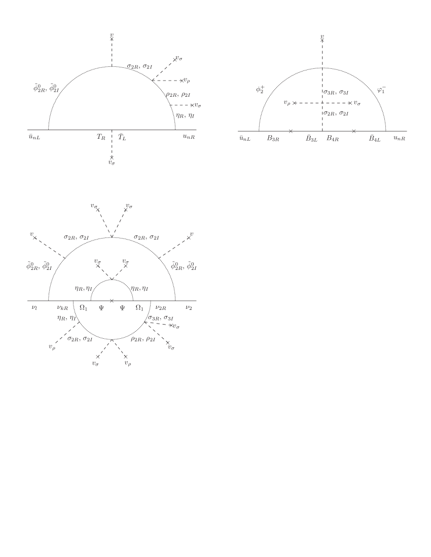
Figure 1: Some of the one-, two- and three-loop Feynman diagrams contributing to the entries of the SM fermion mass matrices. Here, $n,m=1,2$, $l,n=1,3$.

III Constraints on the $Z^{\prime}$ mass, couplings and production at the LHC

In this section, we discuss the constraints on the $Z^{\prime}$ mass and couplings in our model that emerge due to the $2.6\sigma$ lepton universality anomaly expressed as the ratio $R_{K}=\frac{Br\left(B\rightarrow K\mu^{+}\mu^{-}\right)}{Br\left(B\rightarrow Ke^{+}e^{-}\right)}$ measured by the LHCb collaboration. In addition, we will determine the LEP constraint on the $M_{Z^{\prime}}/g_{X}$ ratio. As we will show below, in our model the lepton universality violation is a consequence of the non-universal $U_{1X}$ charge assignments of the fermionic fields. From the $U_{1X}$ assignments for fermions, we find the following $Z^{\prime}$ interactions with the SM fermions:

$$\tciLaplace_{Z`} = g_{X}\overline{q}_{3L}\gamma^{\mu}q_{3L}Z_{\mu}^{\prime}+2g_{X}\sum_{j=1}^{3}\overline{u}_{jR}\gamma^{\mu}u_{jR}Z_{\mu}^{\prime}-g_{X}\sum_{j=1}^{3}\overline{d}_{jR}\gamma^{\mu}d_{jR}Z_{\mu}^{\prime}$$ (2)

$$-3g_{X}\overline{l}_{2L}\gamma^{\mu}l_{2L}Z_{\mu}^{\prime}-6g_{X}\overline{l}_{2R}\gamma^{\mu}l_{2R}Z_{\mu}^{\prime}-3g_{X}\sum_{k=1,3}\overline{l}_{kR}\gamma^{\mu}l_{kR}Z_{\mu}^{\prime}\,.$$

Then the non-universal $Z^{\prime}$ interactions with the SM fermions given above lead to the following effective Hamiltonian, where the fermionic fields are given in the physical basis:

$$\Delta H_{eff} = -\frac{g_{X}^{2}}{M_{Z^{\prime}}^{2}}\left(V_{DL}^{\ast}\right)_{32}\left(V_{DL}\right)_{33}x_{q_{3L}}\sum_{j=1}^{3}\left[x_{l_{jL}}\left(\overline{s}\gamma^{\mu}P_{L}b\right)\left(\overline{l}_{jL}\gamma^{\mu}l_{jL}\right)+x_{l_{jR}}\left(\overline{s}\gamma^{\mu}P_{L}b\right)\left(\overline{l}_{jR}\gamma^{\mu}l_{jR}\right)\right]$$ (3)

$$= -\frac{g_{X}^{2}}{M_{Z^{\prime}}^{2}}\left(V_{DL}^{\ast}\right)_{32}\left(V_{DL}\right)_{33}\left[-3\left(\overline{s}\gamma^{\mu}P_{L}b\right)\left(\overline{l}_{2L}\gamma^{\mu}l_{2L}\right)-6\left(\overline{s}\gamma^{\mu}P_{L}b\right)\left(\overline{l}_{2R}\gamma^{\mu}l_{2R}\right)\right.$$

$$-\left.3\left(\overline{s}\gamma^{\mu}P_{L}b\right)\left(\overline{l}_{1R}\gamma^{\mu}l_{1R}\right)-3\left(\overline{s}\gamma^{\mu}P_{L}b\right)\left(\overline{l}_{3R}\gamma^{\mu}l_{3R}\right)\right]$$

$$\supset \frac{9g_{X}^{2}}{2M_{Z^{\prime}}^{2}}\left(V_{DL}^{\ast}\right)_{32}\left(V_{DL}\right)_{33}\left(\overline{s}\gamma^{\mu}P_{L}b\right)\left(\overline{\mu}\gamma^{\mu}\mu\right)\,,$$

where the following relations have been taken into account:

$$\widetilde{M}_{f} = \left(M_{f}\right)_{diag}=V_{fL}^{\dagger}M_{f}V_{fR},\hskip 28.45274pt\hskip 28.45274ptf_{\left(L,R\right)}=V_{f\left(L,R\right)}\widetilde{f}_{\left(L,R\right)},$$

$$\overline{f}_{iL}\left(M_{f}\right)_{ij}f_{jR} = \overline{\widetilde{f}}_{kL}\left(V_{fL}^{\dagger}\right)_{ki}\left(M_{f}\right)_{ij}\left(V_{fR}\right)_{jl}\widetilde{f}_{lR}=\overline{\widetilde{f}}_{kL}\left(V_{fL}^{\dagger}M_{f}V_{fR}\right)_{kl}\widetilde{f}_{lR}=\overline{\widetilde{f}}_{kL}\left(\widetilde{M}_{f}\right)_{kl}\widetilde{f}_{lR}=m_{fk}\overline{\widetilde{f}}_{kL}\widetilde{f}_{kR},$$

$$k = 1,2,3\,.$$ (4)

Here, $\widetilde{f}_{k\left(L,R\right)}$ and $f_{k\left(L,R\right)}$ ($k=1,2,3$) are the SM fermionic fields in the mass and interaction bases, respectively.

Parameter	$\frac{\Delta C_{9}^{\mu\mu}}{C_{9}^{SM}}$
Best fit	$-0.21$
$1\sigma$ range	$-0.27$ up to $-0.13$
$2\sigma$ range	$-0.32$ up to $-0.08$

Table 4: Constraints on the $C_{9}^{\mu\mu}$ Wilson coefficient from the LHCb data. Taken from Ref. Hurth:2016fbr .

Let us note that the $R_{K}$ anomaly results from a shift in the Wilson coefficient $C_{9}^{\mu\mu}$ appearing in the following $\Delta B=1$ effective Hamiltonian:

$$\Delta H_{eff}=-\frac{G_{F}\alpha_{em}V_{tb}V_{ts}^{\ast}}{\sqrt{2}\pi}\sum_{\widetilde{l}=e,\mu,\tau}C_{9}^{\widetilde{l}\widetilde{l}}\left(\overline{s}\gamma^{\mu}P_{L}b\right)\left(\overline{\widetilde{l}}\gamma^{\mu}\widetilde{l}\right)\,.$$ (5)

Then, our model predicts the following correction to the $C_{9}^{\mu\mu}$ coefficient relative to its SM value:

$$\Delta C_{9}^{\mu\mu}=-\frac{9g_{X}^{2}}{2M_{Z^{\prime}}^{2}}\left(V_{DL}^{\ast}\right)_{32}\left(V_{DL}\right)_{33}\frac{\sqrt{2}\pi}{G_{F}\alpha_{em}V_{tb}V_{ts}^{\ast}}\simeq-\frac{9g_{X}^{2}}{2M_{Z^{\prime}}^{2}}\frac{\sqrt{2}\pi}{G_{F}\alpha_{em}}\,.$$ (6)

On the other hand, the LHCb data provide the constraints on the $C_{9}^{\mu\mu}$ coefficient given in Table 4. Requiring for the correction to the $C_{9}^{\mu\mu}$ coefficient predicted by our model to be inside the $1\sigma$ and $2\sigma$ experimentally allowed ranges, we find the constraints for the $M_{Z^{\prime}}/g_{X}$ ratio:

$$14\;\mbox{TeV}<\frac{M_{Z^{\prime}}}{g_{X}}<20\;\mbox{TeV}\;\;\mbox{at 1}\sigma,\hskip 28.45274pt\hskip 28.45274pt13\;\mbox{TeV}<\frac{M_{Z^{\prime}}}{g_{X}}<26\;\mbox{TeV}\;\;\mbox{at 2}\sigma\,.$$ (7)

With respect to the LEP bounds on the $M_{Z^{\prime}}/g_{X}$ ratio, it is worth mentioning that the tightest constraint arises from the $e^{+}e^{-}\rightarrow\mu^{+}\mu^{-}$ measurement at LEP. Using the effective leptonic interactions

$$\tciLaplace_{eff} = -\frac{g_{X}^{2}}{M_{Z^{\prime}}^{2}}\sum_{j=1}^{3}\left[x_{l_{1L}}x_{l_{jL}}\left(\overline{l}_{1}\gamma^{\mu}P_{L}l_{1}\right)\left(\overline{l}_{jL}\gamma^{\mu}l_{jL}\right)+x_{l_{1L}}x_{l_{jR}}\left(\overline{l}_{1}\gamma^{\mu}P_{L}l_{1}\right)\left(\overline{l}_{jR}\gamma^{\mu}l_{jR}\right)\right]$$ (8)

$$-\frac{g_{X}^{2}}{M_{Z^{\prime}}^{2}}\sum_{j=1}^{3}\left[x_{l_{1R}}x_{l_{jL}}\left(\overline{l}_{1}\gamma^{\mu}P_{R}l_{1}\right)\left(\overline{l}_{jL}\gamma^{\mu}l_{jL}\right)+x_{l_{1R}}x_{l_{jR}}\left(\overline{l}_{1}\gamma^{\mu}P_{R}l_{1}\right)\left(\overline{l}_{jR}\gamma^{\mu}l_{jR}\right)\right]\,,$$

we find that the $e^{+}e^{-}\rightarrow\mu^{+}\mu^{-}$ measurement at LEP imposes the following limit Schael:2013ita :

$$\frac{2M_{Z^{\prime}}}{g_{X}\sqrt{x_{l_{1L}}x_{l_{2L}}+x_{l_{1R}}x_{l_{2R}}+x_{l_{1R}}x_{l_{2L}}+x_{l_{1L}}x_{l_{2R}}}}>4.6\;\mbox{TeV}\,,$$ (9)

which for the leptonic charge assignments of our model takes the form:

$$\frac{2M_{Z^{\prime}}}{3\sqrt{3}g_{X}}\simeq 0.38\frac{M_{Z^{\prime}}}{g_{X}}>4.6\;\mbox{TeV}\,.$$ (10)

The latter yields the following lower bound on the $M_{Z^{\prime}}/g_{X}$ ratio:

$$\frac{M_{Z^{\prime}}}{g_{X}}>12\;\mbox{TeV}\,.$$ (11)

In what follows, we proceed with computing the total cross section for production of a heavy $Z^{\prime}$ gauge boson at the LHC via a  Drell-Yan (DY) mechanism. In this computation, we consider the dominant contribution due to the parton distribution functions of the light up, down and strange quarks, so that the total $Z^{\prime}$ production cross section via quark-antiquark annihilation in proton-proton collisions with center-of-mass energy $\sqrt{S}$ reads:

$$\sigma_{pp\rightarrow Z^{\prime}}^{\mathrm{DY}}\left(S\right) = \frac{g^{2}\pi}{6c_{W}^{2}S}\left\{4g_{X}^{2}\int_{\ln\sqrt{\frac{M_{Z^{\prime}}^{2}}{S}}}^{-\ln\sqrt{\frac{M_{Z^{\prime}}^{2}}{S}}}f_{p/u}\left(\sqrt{\frac{M_{Z^{\prime}}^{2}}{S}}e^{y},\mu^{2}\right)f_{p/\overline{u}}\left(\sqrt{\frac{M_{Z^{\prime}}^{2}}{S}}e^{-y},\mu^{2}\right)dy\right.$$ (12)

$$+\left.g_{X}^{2}\int_{\ln\sqrt{\frac{M_{Z^{\prime}}^{2}}{S}}}^{-\ln\sqrt{\frac{M_{Z^{\prime}}^{2}}{S}}}f_{p/d}\left(\sqrt{\frac{M_{Z^{\prime}}^{2}}{S}}e^{y},\mu^{2}\right)f_{p/\overline{d}}\left(\sqrt{\frac{M_{Z^{\prime}}^{2}}{S}}e^{-y},\mu^{2}\right)dy\right.$$

$$+\left.g_{X}^{2}\int_{\ln\sqrt{\frac{M_{Z^{\prime}}^{2}}{S}}}^{-\ln\sqrt{\frac{M_{Z^{\prime}}^{2}}{S}}}f_{p/s}\left(\sqrt{\frac{M_{Z^{\prime}}^{2}}{S}}e^{y},\mu^{2}\right)f_{p/\overline{s}}\left(\sqrt{\frac{M_{Z^{\prime}}^{2}}{S}}e^{-y},\mu^{2}\right)dy\right\}\,,$$

where $f_{p/u}\left(x_{1},\mu^{2}\right)$ ($f_{p/\overline{u}}\left(x_{2},\mu^{2}\right)$), $f_{p/d}\left(x_{1},\mu^{2}\right)$ ($f_{p/\overline{d}}\left(x_{2},\mu^{2}\right)$) and $f_{p/s}\left(x_{1},\mu^{2}\right)$ ($f_{p/\overline{s}}\left(x_{2},\mu^{2}\right)$) are the distributions of the light up, down and strange quarks (antiquarks) in the proton, respectively, which carry momentum fractions $x_{1}$ ($x_{2}$) of the proton. Here, $\mu=m_{Z^{\prime}}$ is the corresponding factorization scale.

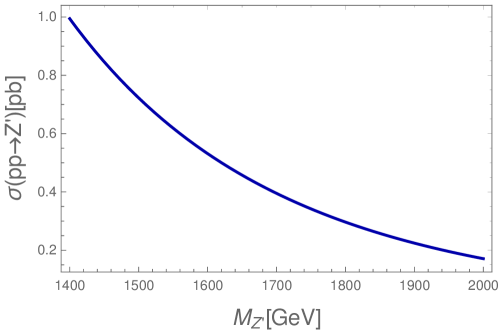
Figure 2: The total $Z^{\prime}$ production cross section via the DY mechanism at the LHC for $\sqrt{S}=13$ TeV and $g_{X}=0.1$ as a function of the $Z^{\prime}$ mass.

Figure 2 displays the total $Z^{\prime}$ production cross section via the DY mechanism at the LHC for $\sqrt{S}=13$ TeV and $g_{X}=0.1$ as a function of the $Z^{\prime}$ mass. The latter is varied from $1.4$ TeV up to $2$ TeV to satisfy the LEP constraint as well as the constraints imposed by the $2.6\sigma$ anomaly in lepton universality. For such as a region of $Z^{\prime}$ masses, we find that the total production cross section is found to be $0.2-1$ pb. On the other hand, at a future $100$ TeV proton-proton collider this cross section gets significantly enhanced reaching values of $9-29$ pb in the same mass interval, as indicated in Figure 3.

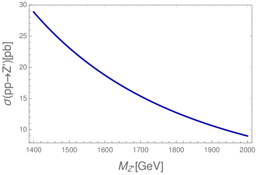
Figure 3: The total $Z^{\prime}$ production cross section via the DY mechanism at a future $pp$ collider for $\sqrt{S}=100$ TeV and $g_{X}=0.1$ as a function of the $Z^{\prime}$ mass.

Note that the dominant $Z^{\prime}$ production channel in pp collisions is via the Drell-Yan process $q\bar{q}\rightarrow Z^{\prime}$, $q=u,d,s$ (for the production cross section see Eq. (12)). The produced $Z^{\prime}$ then can decay into a leptonic pair $Z^{\prime}\rightarrow l\bar{l}$ which is a standard search channel for $Z^{\prime}$ at the LHC. Non-observation of such a decay channel at LEP-II yields the lower bound $M_{{}^{\prime}}/g_{X}>12$ TeV (see Eq. (11)). The hadron collider observables of $Z^{\prime}$ in hadronic and leptonic channels in the current model requires a dedicated analysis of the experimental bounds in each of the $Z^{\prime}$ decay channels, and should be left for future studies.

Finally, to close this section, we justify why our model is safe against Flavor Changing Neutral Currents (FCNCs) constraints. Since the model contains two electroweak doublet Higgs scalars $\phi_{1,2}$ we are required to take special care of this issue. Our model automatically implements the alignment limit for the lightest 125 GeV Higgs boson, because all other scalar states decouple in the mass spectrum and, hence, are very heavy by default. This means the SM-like Higgs boson does not have tree-level FCNCs while such contributions from the heavier scalars are strongly suppressed by their large mass scale. While a detailed study of the FCNC constraints goes beyond the scope of the present work, we can resort to the Glashow-Weinberg-Paschos the theorem Glashow:1976nt ; Paschos:1976ay in order to justify nonexistence of FCNCs in our model. This theorem states that there will be no tree-level FCNC coming from the scalar sector, if all right-handed fermions of a given electric charge couple to only one of the doublets. As seen from Eq. (1) this condition is satisfied in our model. So, despite of an obvious mass suppression, any possible FCNC corrections would emerge at a loop level only, guarantying the model to be safe with respect to the corresponding phenomenological constraints. Finally, any possible FCNC from the $Z^{\prime}$ mediation would be strongly suppressed by its large mass scale compared to the EW one, i.e. $m_{Z^{\prime}}>12$ TeV (for $g_{X}=1$), according to the LEP constraint.

IV Muon anomalous magnetic moment

In this section, we will determine the constraints on the parameter space of our model imposed by the experimental measurements of the muon anomalous magnetic moment. The latter receives one-loop contributions from vertex diagrams involving the $Z^{\prime}$ exchange as well as the exchanges of the heavy $Z_{2}^{\left(2\right)}$ charged neutral scalars $\mathop{\mathrm{R}e}\left(\rho_{1}\right)$, $\mathop{\mathrm{R}e}\left(\phi_{2}^{0}\right)$, $\mathop{\mathrm{I}m}\left(\phi_{2}^{0}\right)$, $\mathop{\mathrm{I}m}\left(\rho_{1}\right)$, that couple to the charged exotic lepton $E_{2}$. The scalar contributions to the muon anomalous magnetic moment include the Yukawa interactions $\overline{E}_{2L}\rho_{1}l_{2R}$ and $\overline{l}_{2L}\phi_{2}E_{2R}$ as well as the trilinear scalar interactions such as $\rho_{2}\left(\phi_{1}\cdot\phi_{2}^{\dagger}\right)\sigma_{1}^{\ast}$ giving rise to the $\phi_{2}^{0}$-$\rho_{2}$ mixing, which is crucial to generate those contributions.

In view of a huge amount of free parameters in the scalar potential of our model (which is shown explicitly in our previous work in Ref. CarcamoHernandez:2019cbd ), for the sake of simplicity, here we work with a simplified benchmark scenario where $\mathop{\mathrm{R}e}\left(\rho_{1}\right)$ ($\mathop{\mathrm{I}m}\left(\rho_{1}\right)$) and $\mathop{\mathrm{R}e}\left(\phi_{2}^{0}\right)$ ($\mathop{\mathrm{I}m}\left(\phi_{2}^{0}\right)$) mix between themselves only and do not mix with other scalar fields. In this scenario, we have the following relations:

$$\left(\begin{array}[]{c}H_{1}\\ H_{2}\end{array}\right)=\left(\begin{array}[]{cc}\cos\theta_{S}&\sin\theta_{S}\\ -\sin\theta_{S}&\cos\theta_{S}\end{array}\right)\left(\begin{array}[]{c}\mathop{\mathrm{R}e}\left(\rho_{1}\right)\\ \mathop{\mathrm{R}e}\left(\phi_{2}^{0}\right)\end{array}\right),\hskip 28.45274pt\hskip 28.45274pt\left(\begin{array}[]{c}A_{1}\\ A_{2}\end{array}\right)=\left(\begin{array}[]{cc}\cos\theta_{P}&\sin\theta_{P}\\ -\sin\theta_{P}&\cos\theta_{P}\end{array}\right)\left(\begin{array}[]{c}\mathop{\mathrm{I}m}\left(\rho_{1}\right)\\ \mathop{\mathrm{I}m}\left(\phi_{2}^{0}\right)\end{array}\right)$$ (13)

where $H_{1}$, $H_{2}$ are the physical CP-even scalars whereas $A_{1}$ and $A_{2}$ are the CP-odd scalars in the physical basis. In addition, without any loss of generality we set $\theta_{S}=\theta_{P}=\theta$ and $y_{22}^{\left(l\right)}=x_{22}^{\left(l\right)}=y$. Then, the muon anomalous magnetic moment in this scenario reads:

$$\Delta a_{\mu} = y^{2}\frac{m_{\mu}^{2}}{8\pi^{2}}\left[I_{S}\left(m_{E_{2}},m_{H_{1}}\right)-I_{S}\left(m_{E_{2}},m_{H_{2}}\right)+I_{P}\left(m_{E_{2}},m_{A_{1}}\right)-I_{P}\left(m_{E_{2}},m_{A_{2}}\right)\right]\sin\theta\cos\theta+\frac{m_{\mu}^{2}}{8\pi^{2}M_{Z^{\prime}}^{2}}I_{V}\left(M_{Z^{\prime}}\right)\,,$$

where the loop integrals are given by Diaz:2002uk ; Kelso:2014qka :

$$I_{S\left(P\right)}\left(m_{E},m\right) = \int_{0}^{1}\frac{x^{2}\left(1-x\pm\frac{m_{E}}{m_{\mu}}\right)}{m_{\mu}^{2}x^{2}+\left(m_{E}^{2}-m_{\mu}^{2}\right)x+m^{2}\left(1-x\right)}dx,$$

$$I_{V}\left(M_{Z^{\prime}}\right) = \int_{0}^{1}\frac{g_{V}^{2}P_{V}\left(x\right)+g_{A}^{2}P_{A}\left(x\right)}{\left(1-x\right)\left(1-\frac{m_{\mu}^{2}}{M_{Z^{\prime}}^{2}}x\right)+\frac{m_{\mu}^{2}}{M_{Z^{\prime}}^{2}}x}dx,\hskip 28.45274pt$$

$$P_{V}\left(x\right) = 2x^{2}\left(1-x\right),\hskip 28.45274pt\hskip 28.45274ptP_{A}\left(x\right)=2x^{2}\left(1-x\right)\left(x-4\right)-4\frac{m_{\mu}^{2}}{M_{Z^{\prime}}^{2}}x^{3}$$

$$g_{L} = -3g_{X},\hskip 28.45274pt\hskip 28.45274ptg_{L}=-6g_{X},\hskip 28.45274pt\hskip 28.45274ptg_{V,A}=g_{R}\pm g_{L}\,.$$ (15)

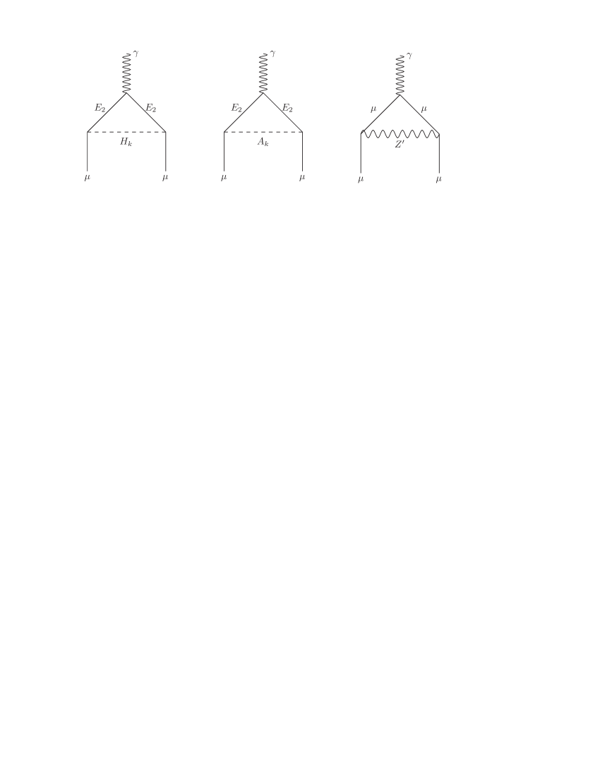
Figure 4: Loop Feynman diagrams contributing to the muon anomalous magnetic moment. Here $k=1,2$

In our numerical analysis we have fixed $\tan\theta=\frac{v}{v_{\sigma}}$, $M_{Z^{\prime}}=1.5$ TeV and $g_{X}=0.1$, in consistency with the $2.6\sigma$ $R_{K}$ anomaly. Considering that the muon anomalous magnetic moment is constrained to be in the range Hagiwara:2011af ; Nomura:2018lsx ; Nomura:2018vfz ,

$$\left(\Delta a_{\mu}\right)_{\exp}=\left(26.1\pm 8\right)\times 10^{-10}\,,$$ (16)

we plot in Figure 5 the allowed parameter space for $M_{S}$-$M_{E}$ (left panel) and $M_{A}$-$M_{E}$ (right panel) planes with different values for $\Delta a_{\mu}$. Here, we have set $M_{S}=\min\left(m_{H_{1}},m_{H_{2}}\right)$ and $M_{A}=\min\left(m_{A_{1}},m_{A_{2}}\right)$ and $M_{E}=m_{E_{2}}$. We found that our model can accommodate the experimental values of $\Delta a_{\mu}$ for a large region of parameter space.

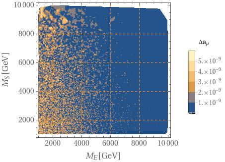
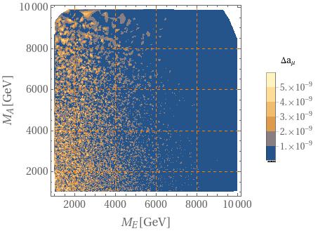
Figure 5: Allowed parameter space for $M_{S}$-$M_{E}$ (left panel) and $M_{A}$-$M_{E}$ (right panel) planes with different values of the muon anomalous magnetic moment.

V DM particle candidates

Note that due to the exact $Z_{2}^{(2)}$ discrete symmetry, our model has several stable scalar DM (DM) candidates, which can be the neutral components of the inert $SU_{2L}$ scalar doublet $\phi_{2}$ as well as the real and imaginary parts of the SM scalar singlets $\sigma_{2}$, $\sigma_{3}$, $\rho_{1}$, $\rho_{2}$ and $\eta$. Furthermore, the model can have a fermionic DM candidate, which is the only SM-singlet Majorana neutrino $\Omega_{1R}$ with a non-trivial $Z_{2}^{(2)}$ charge.

Considering a scenario with a scalar DM candidate, one has to ensure its stability. This can be done by assuming that it is the lightest among the inert scalar particles and is lighter than the exotic fermions. That scalar DM candidate annihilates mainly into $WW$, $ZZ$, $t\overline{t}$, $b\overline{b}$ and $hh$ via a Higgs portal scalar interaction $\left(\phi^{\dagger}_{1}\phi_{1}\right)\Phi^{\dagger}_{DM}\Phi_{DM}$, where $\phi_{1}$ is the SM Higgs doublet and $\Phi_{DM}$ the scalar DM candidate in our model. These annihilation channels will contribute to the DM relic density, which can be accommodated for appropriate values of the scalar DM mass and of the quartic scalar coupling of the corresponding Higgs portal scalar interaction $\left(\phi^{\dagger}_{1}\phi_{1}\right)\Phi^{\dagger}_{DM}\Phi_{DM}$, similarly as in Refs. CarcamoHernandez:2016pdu ; Bernal:2017xat ; CarcamoHernandez:2017kra ; Long:2018dun . Thus, for DM direct detection prospects, the scalar DM candidate would scatter off a nuclear target in a detector via Higgs boson exchange in the $t$-channel, giving rising to a constraint on the coupling of the $\left(\phi^{\dagger}_{1}\phi_{1}\right)\Phi^{\dagger}_{DM}\Phi_{DM}$ interaction. Given the large number of parameters in the scalar potential of our model (which is discussed in detail in our previous work CarcamoHernandez:2019cbd ), there is a lot of parametric freedom that allows us to reproduce

the observed value of the DM relic density and the parameter space of our model consistent with DM constraints will be similar to the one in Refs. CarcamoHernandez:2016pdu ; Bernal:2017xat ; CarcamoHernandez:2017kra ; Long:2018dun .

For instance, in the case, where $m_{{\Phi_{DM}}}^{2}>>v^{2}$, with $v=246$ GeV, and neglecting the annihilation channel of the scalar DM candidate into neutrino-antineutrino pairs as in Ref. Bernal:2017xat , the freeze-out of heavy scalar DM particle will be largely dominated by the annihilations into Higgs bosons and the corresponding thermally averaged cross section can be estimated as

$$<\sigma v>\simeq\frac{\gamma^{2}}{128\pi m_{{\Phi_{DM}}}^{2}},$$ (17)

which results in a DM relic abundance

$$\frac{\Omega_{DM}h^{2}}{0.12}=\frac{0.1pb}{0.12<\sigma v>}\simeq\left(\frac{1}{\gamma}\right)^{2}\left(\frac{m_{{\Phi_{DM}}}}{1.1TeV}\right)^{2},$$ (18)

with $\gamma$ being the quartic scalar coupling of the Higgs portal scalar interaction $\left(\phi^{\dagger}_{1}\phi_{1}\right)\Phi^{\dagger}_{DM}\Phi_{DM}$. Consequently, our model naturally reproduces the observed value Ade:2015xua

$$\Omega_{DM}h^{2}=0.1198$$ (19)

for the DM relic density.

In the scenario with a fermionic DM candidate, it follows from the Yukawa interactions $\overline{\Omega_{1R}^{C}}\eta^{\ast}\nu_{kR}$ and $\overline{\Omega_{1R}^{C}}\eta\Psi_{R}$ that the DM candidate $\Omega_{1R}$ can annihilate into a pair of the right-handed Majorana neutrinos $\nu_{kR}$ ($k=1,3$) and $\Psi_{R}$, via $t$ channel exchange of the real and imaginary parts of the gauge singlet scalar $\eta$. Additionally, the fermionic DM candidate $\Omega_{1R}$ can also annihilate into $\eta_{R}\eta_{R}$ and $\eta_{I}\eta_{I}$ via the the $t$ channel exchange of the right handed Majorana neutrinos $\nu_{kR}$ ($k=1,3$) and $\Psi_{R}$. Thus, the corresponding relic density will depend on the neutrino Yukawa coupling of the aforementioned Yukawa interactions, on the fermionic DM candidate mass $m_{\Omega_{1R}}$, on the masses of the the right-handed Majorana neutrinos $\nu_{kR}$ ($k=1,3$), $\Psi_{R}$, as well as on the masses of the real and imaginary parts of the gauge singlet scalar $\eta$.

Considering a scenario where $m_{{\Omega_{1R}}}^{2}{<<}m_{{\ \eta_{R}}}^{2}\sim m_{{\eta_{I}}}^{2}\sim m_{{\eta}}^{2}$, and the annihilation channel $\Omega_{1R}\Omega_{1R}\rightarrow\nu_{kR}\nu_{kR}$ ($k=1,3$), following Ref. Bernal:2017xat one can estimate the corresponding thermally averaged cross section as

$$<\sigma v>\simeq\frac{9y_{\Omega}^{4}m_{{\Omega}}^{2}}{16\pi m_{{\eta}}^{4}}.$$ (20)

Then, the DM relic abundance is

$$\frac{\Omega_{DM}h^{2}}{0.12}=\frac{0.1pb}{0.12<\sigma v>}\simeq\left(\frac{1}{y_{\Omega}}\right)^{4}\left(\frac{400GeV}{m_{{\Omega}}}\right)^{2}\left(\frac{m_{{\eta}}}{1.9TeV}\right)^{4},$$ (21)

showing that in the case of fermionic DM candidate our model also naturally reproduces the observed value (19).

VI Conclusions

We have studied some phenomenological aspects of the extended Inert Higgs Doublet model, which incorporates the mechanism of sequential loop-generation of the SM fermion masses, explaining the observed strong hierarchies between them as well as the corresponding mixing parameters. A particular emphasis has been made on analyzing the constraints on the $Z^{\prime}$ mass and couplings of our model, imposed by the $2.6\sigma$ anomaly in lepton universality, the LEP constraint on the $M_{Z^{\prime}}/g_{X}$ ratio and the constraints arising from the experimental measurements of the muon anomalous magnetic moment. Furthermore, we have studied production of the heavy $Z^{\prime}$ gauge boson in proton-proton collisions via the Drell-Yan mechanism. We found that the corresponding total cross section at the LHC is equal to $0.2-1$ pb when the heavy $Z^{\prime}$ mass is varied within $1.5-2$ TeV interval for the $U_{1X}$ gauge coupling $g_{X}=0.1$. The $Z^{\prime}$ production cross section gets significantly enhanced at a future $100$ TeV proton-proton collider reaching the typical values of $9-29$ pb. Additionally, we have found that the $2.6\sigma$ anomaly in lepton universality yields a tighter constraint than the one obtained from the $e^{+}e^{-}\rightarrow\mu^{+}\mu^{-}$ measurement at LEP and implies a lower bound of $\approx 13$ TeV on the $M_{Z^{\prime}}/g_{X}$ ratio. We have found that our model successfully accommodates the experimental values of the muon magnetic moment for a large region of parameter space. Finally, we have examined the possible fermion and scalar DM particle candidates of the model and showed that in both cases our predictions are compatible with the observed DM relic density abundance.

Acknowledgements This research has received funding from Fondecyt (Chile) grants No. 1170803, No. 1190845, No. 1180232, No. 3150472 and the UTFSM grant PIM175. R.P. is partially supported by the Swedish Research Council, contract numbers 621-2013-4287 and 2016-05996, by CONICYT grant MEC80170112, as well as by the European Research Council (ERC) under the European Union’s Horizon 2020 research and innovation programme (grant agreement No 668679). This work was supported in part by the Ministry of Education, Youth and Sports of the Czech Republic, project LTC17018. A.E.C.H thanks University of Lund, where part of this work was done, for hospitality as well as University of Southampton and Institute of Experimental and Applied Physics of the Czech Technical University in Praga for hospitality during the completion of this work.

References

- (1) M. D. Campos, A. E. Cárcamo Hernández, H. Pas and E. Schumacher, Phys. Rev. D 91, no. 11, 116011 (2015) doi:10.1103/PhysRevD.91.116011 [arXiv:1408.1652 [hep-ph]].
- (2) A. E. Cárcamo Hernández, Eur. Phys. J. C 76, no. 9, 503 (2016) doi:10.1140/epjc/s10052-016-4351-y [arXiv:1512.09092 [hep-ph]].
- (3) A. E. Cárcamo Hernández, I. de Medeiros Varzielas and E. Schumacher, Phys. Rev. D 93, no. 1, 016003 (2016) doi:10.1103/PhysRevD.93.016003 [arXiv:1509.02083 [hep-ph]].
- (4) C. Arbeláez, A. E. Cárcamo Hernández, S. Kovalenko and I. Schmidt, Eur. Phys. J. C 77, no. 6, 422 (2017) doi:10.1140/epjc/s10052-017-4948-9 [arXiv:1602.03607 [hep-ph]].
- (5) S. F. Mantilla, R. Martinez and F. Ochoa, Phys. Rev. D 95, no. 9, 095037 (2017) doi:10.1103/PhysRevD.95.095037 [arXiv:1612.02081 [hep-ph]].
- (6) N. Bernal, A. E. Cárcamo Hernández, I. de Medeiros Varzielas and S. Kovalenko, JHEP 1805, 053 (2018) doi:10.1007/JHEP05(2018)053 [arXiv:1712.02792 [hep-ph]].
- (7) A. E. Cárcamo Hernández, S. Kovalenko and I. Schmidt, JHEP 1702, 125 (2017) doi:10.1007/JHEP02(2017)125 [arXiv:1611.09797 [hep-ph]].
- (8) A. E. Cárcamo Hernández, S. Kovalenko, H. N. Long and I. Schmidt, JHEP 1807, 144 (2018) doi:10.1007/JHEP07(2018)144 [arXiv:1705.09169 [hep-ph]].
- (9) S. F. Mantilla and R. Martinez, Phys. Rev. D 96, no. 9, 095027 (2017) doi:10.1103/PhysRevD.96.095027 [arXiv:1704.04869 [hep-ph]].
- (10) G. Abbas, arXiv:1712.08052 [hep-ph].
- (11) A. Dev and R. N. Mohapatra, Phys. Rev. D 98, no. 7, 073002 (2018) doi:10.1103/PhysRevD.98.073002 [arXiv:1804.01598 [hep-ph]].
- (12) A. E. Cárcamo Hernández, S. Kovalenko, J. W. F. Valle and C. A. Vaquera-Araujo, JHEP 1902, 065 (2019) doi:10.1007/JHEP02(2019)065 [arXiv:1811.03018 [hep-ph]].
- (13) G. Abbas, arXiv:1807.05683 [hep-ph].
- (14) A. E. Cárcamo Hernández, J. Marchant González and U. J. Saldaña-Salazar, arXiv:1904.09993 [hep-ph].
- (15) A. E. Cárcamo Hernández, Y. Hidalgo Velásquez and N. A. Pérez-Julve, arXiv:1905.02323 [hep-ph].
- (16) A. E. Cárcamo Hernández, S. Kovalenko, R. Pasechnik and I. Schmidt, arXiv:1901.02764 [hep-ph].
- (17) A. Vicente, Adv. High Energy Phys. 2018, 3905848 (2018) doi:10.1155/2018/3905848 [arXiv:1803.04703 [hep-ph]].
- (18) A. Crivellin, L. Hofer, J. Matias, U. Nierste, S. Pokorski and J. Rosiek, Phys. Rev. D 92 (2015) no.5, 054013 doi:10.1103/PhysRevD.92.054013 [arXiv:1504.07928 [hep-ph]].
- (19) A. Crivellin, G. D’Ambrosio and J. Heeck, Phys. Rev. D 91 (2015) no.7, 075006 doi:10.1103/PhysRevD.91.075006 [arXiv:1503.03477 [hep-ph]].
- (20) S. F. King, JHEP 1809, 069 (2018) doi:10.1007/JHEP09(2018)069 [arXiv:1806.06780 [hep-ph]].
- (21) C. Bonilla, T. Modak, R. Srivastava and J. W. F. Valle, Phys. Rev. D 98, no. 9, 095002 (2018) doi:10.1103/PhysRevD.98.095002 [arXiv:1705.00915 [hep-ph]].
- (22) R. Barbieri and A. Tesi, Eur. Phys. J. C 78, no. 3, 193 (2018) doi:10.1140/epjc/s10052-018-5680-9 [arXiv:1712.06844 [hep-ph]].
- (23) S. F. King, JHEP 1708, 019 (2017) doi:10.1007/JHEP08(2017)019 [arXiv:1706.06100 [hep-ph]].
- (24) M. C. Romao, S. F. King and G. K. Leontaris, arXiv:1710.02349 [hep-ph].
- (25) S. Antusch, C. Hohl, S. F. King and V. Susic, arXiv:1712.05366 [hep-ph].
- (26) P. Ko, T. Nomura and H. Okada, Phys. Lett. B 772, 547 (2017) doi:10.1016/j.physletb.2017.07.021 [arXiv:1701.05788 [hep-ph]].
- (27) P. Ko, T. Nomura and H. Okada, Phys. Rev. D 95, no. 11, 111701 (2017) doi:10.1103/PhysRevD.95.111701 [arXiv:1702.02699 [hep-ph]].
- (28) C. H. Chen, T. Nomura and H. Okada, Phys. Lett. B 774, 456 (2017) doi:10.1016/j.physletb.2017.10.005 [arXiv:1703.03251 [hep-ph]].
- (29) N. Assad, B. Fornal and B. Grinstein, Phys. Lett. B 777, 324 (2018) doi:10.1016/j.physletb.2017.12.042 [arXiv:1708.06350 [hep-ph]].
- (30) A. Angelescu, D. Becirevic, D. A. Faroughy and O. Sumensari, JHEP 1810, 183 (2018) doi:10.1007/JHEP10(2018)183 [arXiv:1808.08179 [hep-ph]].
- (31) L. Di Luzio, J. Fuentes-Martin, A. Greljo, M. Nardecchia and S. Renner, JHEP 1811, 081 (2018) doi:10.1007/JHEP11(2018)081 [arXiv:1808.00942 [hep-ph]].
- (32) D. Guadagnoli, M. Reboud and O. Sumensari, JHEP 1811, 163 (2018) doi:10.1007/JHEP11(2018)163 [arXiv:1807.03285 [hep-ph]].
- (33) B. Fornal, S. A. Gadam and B. Grinstein, arXiv:1812.01603 [hep-ph].
- (34) U. Aydemir, D. Minic, C. Sun and T. Takeuchi, JHEP 1809, 117 (2018) doi:10.1007/JHEP09(2018)117 [arXiv:1804.05844 [hep-ph]].
- (35) T. Faber, M. Hudec, M. Malinsky, P. Meinzinger, W. Porod and F. Staub, Phys. Lett. B 787, 159 (2018) doi:10.1016/j.physletb.2018.10.051 [arXiv:1808.05511 [hep-ph]].
- (36) B. Barman, D. Borah, L. Mukherjee and S. Nandi, arXiv:1808.06639 [hep-ph].
- (37) J. Heeck and D. Teresi, JHEP 1812, 103 (2018) doi:10.1007/JHEP12(2018)103 [arXiv:1808.07492 [hep-ph]].
- (38) B. Grinstein, S. Pokorski and G. G. Ross, JHEP 1812, 079 (2018) [JHEP 2018, 079 (2020)] doi:10.1007/JHEP12(2018)079 [arXiv:1809.01766 [hep-ph]].
- (39) A. Falkowski, S. F. King, E. Perdomo and M. Pierre, JHEP 1808, 061 (2018) doi:10.1007/JHEP08(2018)061 [arXiv:1803.04430 [hep-ph]].
- (40) A. E. Cárcamo Hernández and S. F. King, arXiv:1803.07367 [hep-ph].
- (41) I. de Medeiros Varzielas and S. F. King, JHEP 1811, 100 (2018) doi:10.1007/JHEP11(2018)100 [arXiv:1807.06023 [hep-ph]].
- (42) P. Rocha-Moran and A. Vicente, arXiv:1810.02135 [hep-ph].
- (43) Q. Y. Hu, X. Q. Li and Y. D. Yang, arXiv:1810.04939 [hep-ph].
- (44) M. Carena, E. Megias, M. Quiros and C. Wagner, JHEP 1812, 043 (2018) doi:10.1007/JHEP12(2018)043 [arXiv:1809.01107 [hep-ph]].
- (45) K. S. Babu, R. N. Mohapatra and B. Dutta, arXiv:1811.04496 [hep-ph].
- (46) B. C. Allanach and J. Davighi, arXiv:1809.01158 [hep-ph].
- (47) T. Hurth, F. Mahmoudi and S. Neshatpour, Nucl. Phys. B 909, 737 (2016) doi:10.1016/j.nuclphysb.2016.05.022 [arXiv:1603.00865 [hep-ph]].
- (48) S. L. Glashow and S. Weinberg, Phys. Rev. D 15, 1958 (1977). doi:10.1103/PhysRevD.15.1958
- (49) E. A. Paschos, Phys. Rev. D 15, 1966 (1977). doi:10.1103/PhysRevD.15.1966
- (50) S. Schael et al. [ALEPH and DELPHI and L3 and OPAL and LEP Electroweak Collaborations], Phys. Rept. 532, 119 (2013) doi:10.1016/j.physrep.2013.07.004 [arXiv:1302.3415 [hep-ex]].
- (51) R. A. Diaz, R. Martinez and J. A. Rodriguez, Phys. Rev. D 67, 075011 (2003) doi:10.1103/PhysRevD.67.075011 [hep-ph/0208117].
- (52) C. Kelso, H. N. Long, R. Martinez and F. S. Queiroz, Phys. Rev. D 90, no. 11, 113011 (2014) doi:10.1103/PhysRevD.90.113011 [arXiv:1408.6203 [hep-ph]].
- (53) K. Hagiwara, R. Liao, A. D. Martin, D. Nomura and T. Teubner, J. Phys. G 38, 085003 (2011) doi:10.1088/0954-3899/38/8/085003 [arXiv:1105.3149 [hep-ph]].
- (54) T. Nomura and H. Okada, arXiv:1808.05476 [hep-ph].
- (55) T. Nomura and H. Okada, Phys. Rev. D 97, no. 9, 095023 (2018) doi:10.1103/PhysRevD.97.095023 [arXiv:1803.04795 [hep-ph]].
- (56) A. E.Cárcamo Hernández and H. N. Long, J. Phys. G 45, no. 4, 045001 (2018) doi:10.1088/1361-6471/aaace7 [arXiv:1705.05246 [hep-ph]].
- (57) H. N. Long, N. V. Hop, L. T. Hue, N. H. Thao and A. E. Cárcamo Hernández, arXiv:1810.00605 [hep-ph].
- (58) P. A. R. Ade et al. [Planck Collaboration], “Planck 2015 results. XIII. Cosmological parameters,” Astron. Astrophys. 594, A13 (2016) [arXiv:1502.01589 [astro-ph.CO]].