Black Box Submodular Maximization:
Discrete and Continuous Settings

Abstract

In this paper, we consider the problem of black box continuous submodular maximization where we only have access to the function values and no information about the derivatives is provided. For a monotone and continuous DR-submodular function, and subject to a bounded convex body constraint, we propose Black-box Continuous Greedy, a derivative-free algorithm that provably achieves the tight $[(1-1/e)OPT-\epsilon]$ approximation guarantee with $O(d/\epsilon^{3})$ function evaluations. We then extend our result to the stochastic setting where function values are subject to stochastic zero-mean noise. It is through this stochastic generalization that we revisit the discrete submodular maximization problem and use the multi-linear extension as a bridge between discrete and continuous settings. Finally, we extensively evaluate the performance of our algorithm on continuous and discrete submodular objective functions using both synthetic and real data.

1 Introduction

Black-box optimization, also known as zeroth-order or derivative-free optimization, has been extensively studied in the literature (Conn et al., 2009; Bergstra et al., 2011; Rios and Sahinidis, 2013; Shahriari et al., 2016). In this setting, we assume that the objective function is unknown and we can only obtain zeroth-order information such as (stochastic) function evaluations.

Fueled by a growing number of machine learning applications, black-box optimization methods are usually considered in scenarios where gradients (i.e., first-order information) are 1) difficult or slow to compute, e.g., graphical model inference (Wainwright et al., 2008), structure predictions (Taskar et al., 2005; Sokolov et al., 2016), or 2) inaccessible, e.g., hyper-parameter turning for natural language processing or image classifications Snoek et al. (2012); Thornton et al. (2013), black-box attacks for finding adversarial examples Chen et al. (2017c); Ilyas et al. (2018). Even though heuristics such as random or grid search, with undesirable dependencies on the dimension, are still used in some applications (e.g., parameter tuning for deep networks), there has been a growing number of rigorous methods to address the convergence rate of black-box optimization in convex and non-convex settings (Wang et al., 2017; Balasubramanian and Ghadimi, 2018; Sahu et al., 2018).

The focus of this paper is the constrained continuous DR-submodular maximization over a bounded convex body. We aim to design an algorithm that uses only zeroth-order information while avoiding expensive projection operations. Note that one way the optimization methods can deal with constraints is to apply the projection oracle once the proposed iterates land outside the feasibility region. However, computing the projection in many constrained settings is computationally prohibitive (e.g., projection over bounded trace norm matrices, flow polytope, matroid polytope, rotation matrices). In such scenarios, projection-free algorithms, a.k.a., Frank-Wolfe (Frank and Wolfe, 1956), replace the projection with a linear program. Indeed, our proposed algorithm combines efficiently the zeroth-order information with solving a series of linear programs to ensure convergence to a near-optimal solution.

Continuous DR-submodular functions are an important subset of non-convex functions that can be minimized exactly Bach (2016); Staib and Jegelka (2017) and maximized approximately Bian et al. (2017a, b); Hassani et al. (2017); Mokhtari et al. (2018a); Hassani et al. (2019); Zhang et al. (2019b) This class of functions generalize the notion of diminishing returns, usually defined over discrete set functions, to the continuous domains. They have found numerous applications in machine learning including MAP inference in determinantal point processes (DPPs) Kulesza et al. (2012), experimental design Chen et al. (2018c), resource allocation Eghbali and Fazel (2016), mean-field inference in probabilistic models Bian et al. (2018), among many others.

Motivation: Computing the gradient of a continuous DR-submodular function has been shown to be computationally prohibitive (or even intractable) in many applications. For example, the objective function of influence maximization is defined via specific stochastic processes (Kempe et al., 2003; Rodriguez and Schölkopf, 2012) and computing/estimating the gradient of the mutliliear extension would require a relatively high computational complexity. In the problem of D-optimal experimental design , the gradient of the objective function involves inversion of a potentially large matrix (Chen et al., 2018c). Moreover, when one attacks a submodular recommender model, only black-box information is available and the service provider is unlikely to provide additional first-order information (this is known as the black-box adversarial attack model) (Lei et al., 2019).

There has been very recent progress on developing zeroth-order methods for constrained optimization problems in convex and non-convex settings Ghadimi and Lan (2013); Sahu et al. (2018). Such methods typically assume the objective function is defined on the whole $\mathbb{R}^{d}$ so that they can sample points from a proper distribution defined on $\mathbb{R}^{d}$. For DR-submodular functions, this assumption might be unrealistic, since many DR-submodular functions might be only defined on a subset of $\mathbb{R}^{d}$, e.g., the multi-linear extension Vondrák (2008), a canonical example of DR-submodular functions, is only defined on a unit cube. Moreover, they can only guarantee to reach a first-order stationary point. However, Hassani et al. (2017) showed that for a monotone DR-submodular function, the stationary points can only guarantee $1/2$ approximation to the optimum. Therefore, if a state-of-the-art zeroth-order non-convex algorithm is used for maximizing a monotone DR-submodular function, it is likely to terminate at a suboptimal stationary point whose approximation ratio is only $1/2$.

Our contributions: In this paper, we propose a derivative-free and projection-free algorithm Black-box Continuous Greedy (BCG), that maximizes a monotone continuous DR-submodular function over a bounded convex body $\mathcal{K}\subseteq\mathbb{R}^{d}$. We consider three scenarios:

• In the deterministic setting, where function evaluations can be obtained exactly, BCG achieves the tight $[(1-1/e)OPT-\epsilon]$ approximation guarantee with $\mathcal{O}(d/\epsilon^{3})$ function evaluations.

• In the stochastic setting, where function evaluations are noisy, BCG achieves the tight $[(1-1/e)OPT-\epsilon]$ approximation guarantee with $\mathcal{O}(d^{3}/\epsilon^{5})$ function evaluations.

• In the discrete setting, Discrete Black-box Greedy (DBG) achieves the tight $[(1-1/e)OPT-\epsilon]$ approximation guarantee with $\mathcal{O}(d^{5}/\epsilon^{5})$ function evaluations.

Table 1: Number of function queries in different settings, where $D_{1}$ is the diameter of $\mathcal{K}$.

Function	Additional Assumptions	Function Queries
continuous DR-submodular	monotone, $G$-Lip., $L$-smooth	$\mathcal{O}(\max\{G,LD_{1}\}^{3}\cdot\frac{d}{\epsilon^{3}})$ [Theorem 1]
stoch. conti. DR-submodular	monotone, $G$-Lip., $L$-smooth	$\mathcal{O}(\max\{G,LD_{1}\}^{3}\cdot\frac{d^{3}}{\epsilon^{5}})$ [Theorem 2]
discrete submodular	monotone	$\mathcal{O}(\frac{d^{5}}{\epsilon^{5}})$ [Theorem 3]

All the theoretical results are summarized in Table 1.

We would like to note that in discrete setting, due to the conservative upper bounds for the Lipschitz and smooth parameters of general multilinear extensions, and the variance of the gradient estimators subject to noisy function evaluations, the required number of function queries in theory is larger than the best known result, $\mathcal{O}(d^{5/2}/\epsilon^{3})$ in Mokhtari et al. (2018a, b). However, our experiments show that empirically, our proposed algorithm often requires significantly fewer function evaluations and less running time, while achieving a practically similar utility.

Novelty of our work: All the previous results in constrained DR-submodular maximization assume access to (stochastic) gradients. In this work, we address a harder problem, i.e., we provide the first rigorous analysis when only (stochastic) function values can be obtained. More specifically, with the smoothing trick (Flaxman et al., 2005), one can construct an unbiased gradient estimator via function queries. However, this estimator has a large $\mathcal{O}(d^{2}/\delta^{2})$ variance which may cause FW-type methods to diverge. To overcome this issue, we build on the momentum method proposed by Mokhtari et al. (2018a) in which they assumed access to the first-order information.

Given a point $x$, the smoothed version of $F$ at $x$ is defined as $\mathbb{E}_{v\sim B^{d}}[F(x+\delta v)]$. If $x$ is close to the boundary of the domain $\mathcal{D},(x+\delta v)$ may fall outside of $\mathcal{D}$, leaving the smoothed function undefined for many instances of DR-submodular functions (e.g., the multilinear extension is only defined over the unit cube). Thus the vanilla smoothing trick will not work. To this end, we transform the domain $\mathcal{D}$ and constraint set $\mathcal{K}$ in a proper way and run our zeroth-order method on the transformed constraint set $\mathcal{K}^{\prime}$. Importantly, we retrieve the same convergence rate of $\mathcal{O}(T^{-1/3})$ as in Mokhtari et al. (2018a) with a minimum number of function queries in different settings (continuous, stochastic continuous, discrete).

We further note that by using more recent variance reduction techniques (Zhang et al., 2019b), one might be able to reduce the required number of function evaluations.

1.1 Further Related Work

Submodular functions Nemhauser et al. (1978), that capture the intuitive notion of diminishing returns, have become increasingly important in various machine learning applications. Examples include graph cuts in computer vision Jegelka and Bilmes (2011a, b), data summarization Lin and Bilmes (2011b, a); Tschiatschek et al. (2014); Chen et al. (2018a, 2017b), influence maximization Kempe et al. (2003); Rodriguez and Schölkopf (2012); Zhang et al. (2016), feature compression Bateni et al. (2019), network inference Chen et al. (2017a), active and semi-supervised learning Guillory and Bilmes (2010); Golovin and Krause (2011); Wei et al. (2015), crowd teaching Singla et al. (2014), dictionary learning Das and Kempe (2011), fMRI parcellation Salehi et al. (2017), compressed sensing and structured sparsity Bach (2010); Bach et al. (2012), fairness in machine learning Balkanski and Singer (2015); Celis et al. (2016), and learning causal structures Steudel et al. (2010); Zhou and Spanos (2016), to name a few. Continuous DR-submodular functions naturally extend the notion of diminishing returns to the continuous domains Bian et al. (2017b). Monotone continuous DR-submodular functions can be (approximately) maximized over convex bodies using first-order methods Bian et al. (2017b); Hassani et al. (2017); Mokhtari et al. (2018a). Bandit maximization of monotone continuous DR-submodular functions Zhang et al. (2019a) is a closely related setting to ours. However, to the best of our knowledge, none of the existing work has developed a zeroth-order algorithm for maximizing a monotone continuous DR-submodular function. For a detailed review of DFO and BBO, interested readers refer to book (Audet and Hare, 2017).

2 Preliminaries

Submodular Functions

We say a set function $f\mathrel{\mathop{\mathchar 58\relax}}2^{\Omega}\to\mathbb{R}$ is submodular, if it satisfies the diminishing returns property: for any $A\subseteq B\subseteq\Omega$ and $x\in\Omega\setminus B$, we have

$$f(A\cup\{x\})-f(A)\geq f(B\cup\{x\})-f(B).$$ (1)

In words, the marginal gain of adding an element $x$ to a subset $A$ is no less than that of adding $x$ to its superset $B$.

For the continuous analogue, consider a function $F\mathrel{\mathop{\mathchar 58\relax}}\mathcal{X}\to\mathbb{R}_{+}$, where $\mathcal{X}=\Pi_{i=1}^{n}\mathcal{X}_{i}$, and each $\mathcal{X}_{i}$ is a compact subset of $\mathbb{R}_{+}$. We define $F$ to be continuous submodular if $F$ is continuous and for all $x,y\in\mathcal{X}$, we have

$$F(x)+F(y)\geq F(x\vee y)+F(x\wedge y),$$ (2)

where $\vee$ and $\wedge$ are the component-wise maximizing and minimizing operators, respectively.

The continuous function $F$ is called DR-submodular Bian et al. (2017b) if $F$ is differentiable and $\forall\,x\leq y\mathrel{\mathop{\mathchar 58\relax}}\,\nabla F(x)\geq\nabla F(y).$ An important implication of DR-submodularity is that the function $F$ is concave in any non-negative directions, i.e., for $x\leq y$, we have

$$F(y)\leq F(x)+\langle\nabla F(x),y-x\rangle.$$ (3)

The function $F$ is called monotone if for $x\leq y$, we have $F(x)\leq F(y).$

Smoothing Trick

For a function $F$ defined on $\mathbb{R}^{d}$, its $\delta$-smoothed version is given as

$$\tilde{F}_{\delta}(x)\triangleq\mathbb{E}_{v\sim B^{d}}[F(x+\delta v)],$$ (4)

where $v$ is chosen uniformly at random from the $d$-dimensional unit ball $B^{d}$. In words, the function $\tilde{F}_{\delta}$ at any point $x$ is obtained by “averaging” $F$ over a ball of radius $\delta$ around $x$. In the sequel, we omit the subscript $\delta$ for the sake of simplicity and use $\tilde{F}$ instead of $\tilde{F}_{\delta}$.

Lemma 1 below shows that under the Lipschitz assumption for $F$, the smoothed version $\tilde{F}$ is a good approximation of $F$, and also inherits the key structural properties of $F$ (such as monotonicity and submodularity). Thus one can (approximately) optimize $F$ via optimizing $\tilde{F}$.

Lemma 1 (Proof in Appendix A).

If $F$ is monotone continuous DR-submodular and $G$-Lipschitz continuous on $\mathbb{R}^{d}$, then so is $\tilde{F}$ and

$$|\tilde{F}(x)-F(x)|\leq\delta G.$$ (5)

An important property of $\tilde{F}$ is that one can obtain an unbiased estimation for its gradient $\nabla\tilde{F}$ by a single query of $F$. This property plays a key role in our proposed derivative-free algorithms.

Lemma 2 (Lemma 6.5 in (Hazan, 2016)).

Given a function $F$ on $\mathbb{R}^{d}$, if we choose $u$ uniformly at random from the $(d-1)$-dimensional unit sphere $S^{d-1}$, then we have

$$\nabla\tilde{F}(x)=\mathbb{E}_{u\sim S^{d-1}}\left[\frac{d}{\delta}F(x+\delta u)u\right].$$ (6)

3 DR-Submodular Maximization

In this paper, we mainly focus on the constrained optimization problem:

$$\max_{x\in\mathcal{K}}F(x),$$ (7)

where $F$ is a monotone continuous DR-submodular function on $\mathbb{R}^{d}$, and the constraint set $\mathcal{K}\subseteq\mathcal{X}\subseteq\mathbb{R}^{d}$ is convex and compact.

For first-order monotone DR-submodular maximization, one can use Continuous Greedy Calinescu et al. (2011); Bian et al. (2017b), a variant of Frank-Wolfe Algorithm (Frank and Wolfe, 1956; Jaggi, 2013; Lacoste-Julien and Jaggi, 2015), to achieve the $[(1-1/e)OPT-\epsilon]$ approximation guarantee. At iteration $t$, the FW variant first maximizes the linearization of the objective function $F$:

$$v_{t}=\operatorname*{arg\,max}_{v\in\mathcal{K}}\langle v,\nabla F(x_{t})\rangle.$$ (8)

Then the current point $x_{t}$ moves in the direction of $v_{t}$ with a step size $\gamma_{t}\in(0,1]$:

$$x_{t+1}=x_{t}+\gamma_{t}v_{t}.$$ (9)

Hence, by solving linear optimization problems, the iterates are updated without resorting to the projection oracle.

Here we introduce our main algorithm Black-box Continuous Greedy which assumes access only to function values (i.e., zeroth-order information). This algorithm is partially based on the idea of Continuous Greedy. The basic idea is to utilize the function evaluations of $F$ at carefully selected points to obtain unbiased estimations of the gradient of the smoothed version, $\nabla\tilde{F}$. By extending Continuous Greedy to the derivative-free setting and using recently proposed variance reduction techniques, we can then optimize $\tilde{F}$ near-optimally. Finally, by Lemma 1 we show that the obtained optimizer also provides a good solution for $F$.

Recall that continuous DR-submodular functions are defined on a box $\mathcal{X}=\Pi_{i=1}^{n}\mathcal{X}_{i}$. To simplify the exposition, we can assume, without loss of generality, that the objective function $F$ is defined on $\mathcal{D}\triangleq\prod_{i=1}^{d}[0,a_{i}]$ Bian et al. (2017a). Moreover, we note that since $\tilde{F}=\mathbb{E}_{v\sim B^{d}}[F(x+\delta v)]$, for $x$ close to $\partial\mathcal{D}$ (the boundary of $\mathcal{D}$), the point $x+\delta v$ may fall outside of $\mathcal{D}$, leaving the function $\tilde{F}$ undefined.

To circumvent this issue, we shrink the domain $\mathcal{D}$ by $\delta$. Precisely, the shrunk domain is defined as

$$\mathcal{D}^{\prime}_{\delta}=\{x\in\mathcal{D}|d(x,\partial\mathcal{D})\geq\delta\}.$$ (10)

Since we assume $\mathcal{D}=\prod_{i=1}^{d}[0,a_{i}]$, the shrunk domain is $\mathcal{D}^{\prime}_{\delta}=\prod_{i=1}^{d}[\delta,a_{i}-\delta]$. Then for all $x\in\mathcal{D}^{\prime}_{\delta}$, we have $x+\delta v\in\mathcal{D}$. So $\tilde{F}$ is well-defined on $\mathcal{D}^{\prime}_{\delta}$. By Lemma 1, the optimum of $\tilde{F}$ on the shrunk domain $\mathcal{D}^{\prime}_{\delta}$ will be close to that on the original domain $\mathcal{D}$, if $\delta$ is small enough. Therefore, we can first optimize $\tilde{F}$ on $\mathcal{D}^{\prime}_{\delta}$, then approximately optimize $\tilde{F}$ (and thus $F$) on $\mathcal{D}$. For simplicity of analysis, we also translate the shrunk domain $\mathcal{D}^{\prime}_{\delta}$ by $-\delta$, and denote it as $\mathcal{D}_{\delta}=\prod_{i=1}^{d}[0,a_{i}-2\delta]$.

Besides the domain $\mathcal{D}$, we also need to consider the transformation on constraint set $\mathcal{K}$. Intuitively, if there is no translation, we should consider the intersection of $\mathcal{K}$ and the shrunk domain $\mathcal{D}^{\prime}_{\delta}$. But since we translate $\mathcal{D}^{\prime}_{\delta}$ by $-\delta$, the same transformation should be performed on $\mathcal{K}$. Thus, we define the transformed constraint set as the translated intersection (by $-\delta$) of $\mathcal{D}^{\prime}_{\delta}$ and $\mathcal{K}$:

$$\mathcal{K}^{\prime}\triangleq(\mathcal{D}^{\prime}_{\delta}\cap\mathcal{K})-\delta\mathbf{1}=\mathcal{D}_{\delta}\cap(\mathcal{K}-\delta\mathbf{1}).$$ (11)

It is well known that the FW Algorithm is sensitive to the accuracy of gradient, and may have arbitrarily poor performance with stochastic gradients Hazan and Luo (2016); Mokhtari et al. (2018b). Thus we incorporate two methods of variance reduction into our proposed algorithm Black-box Continuous Greedy which correspond to Step 7 and Step 8 in Algorithm 1, respectively. First, instead of the one-point gradient estimation in Lemma 2, we adopt the two-point estimator of $\nabla\tilde{F}(x)$ (Agarwal et al., 2010; Shamir, 2017):

$$\frac{d}{2\delta}(F(x+\delta u)-F(x-\delta u))u,$$ (12)

where $u$ is chosen uniformly at random from the unit sphere $S^{d-1}$.We note that (12) is an unbiased gradient estimator with less variance w.r.t. the one-point estimator. We also average over a mini-batch of $B_{t}$ independently sampled two-point estimators for further variance reduction. The second variance-reduction technique is the momentum method used in (Mokhtari et al., 2018a) to estimate the gradient by a vector $\bar{g}_{t}$ which is updated at each iteration as follows:

$$\bar{g}_{t}=(1-\rho_{t})\bar{g}_{t-1}+\rho_{t}g_{t}.$$ (13)

Here $\rho_{t}$ is a given step size, $\bar{g}_{0}$ is initialized as an all zero vector $\mathbf{0}$, and $g_{t}$ is an unbiased estimate of the gradient at iterate $x_{t}$. As $\bar{g}_{t}$ is a weighted average of previous gradient approximation $\bar{g}_{t-1}$ and the newly updated stochastic gradient $g_{t}$, it has a lower variance compared with $g_{t}$. Although $\bar{g}_{t}$ is not an unbiased estimation of the true gradient, the error of it will approach zero as time proceeds. The detailed description of Black-box Continuous Greedy is provided in Algorithm 1.

1:  Input: constraint set $\mathcal{K}$, iteration number $T$, radius $\delta$, step size $\rho_{t}$, batch size $B_{t}$

2:  Output: $x_{T+1}+\delta\mathbf{1}$

3:  $x_{1}\leftarrow\mathbf{0},\enspace\bar{g}_{0}\leftarrow\mathbf{0}$

4:  for $t=1$ to $T$ do

5:     Sample $u_{t,1},\dots,u_{t,B_{t}}$ i.i.d. from $S^{d-1}$

6:     For $i=1$ to $B_{t}$, let $y_{t,i}^{+}\leftarrow\delta\mathbf{1}+x_{t}+\delta u_{t,i},y_{t,i}^{-}\leftarrow\delta\mathbf{1}+x_{t}-\delta u_{t,i}$ and evaluate $F(y_{t,i}^{+}),F(y_{t,i}^{-})$

7:     $g_{t}\leftarrow\frac{1}{B_{t}}\sum_{i=1}^{B_{t}}\frac{d}{2\delta}[F(y_{t,i}^{+})-F(y_{t,i}^{-})]u_{t,i}$

8:     $\bar{g}_{t}\leftarrow(1-\rho_{t})\bar{g}_{t-1}+\rho_{t}g_{t}$

9:     $v_{t}\leftarrow\operatorname*{arg\,max}_{v\in\mathcal{K}^{\prime}}\langle v,\bar{g}_{t}\rangle$

10:     $x_{t+1}\leftarrow x_{t}+\frac{v_{t}}{T}$

11:  end for

12:  Output $x_{T+1}+\delta\mathbf{1}$

Algorithm 1 Black-box Continuous Greedy

Theorem 1 (Proof in Appendix B).

For a monotone continuous DR-submodular function $F$, which is also $G$-Lipschitz continuous and $L$-smooth on a convex and compact constraint set $\mathcal{K}$, if we set $\rho_{t}=2/(t+3)^{2/3}$ in Algorithm 1, then we have $\displaystyle(1-1/e)F(x^{*})-\mathbb{E}[F(x_{T+1}+\delta\mathbf{1})]$ $\displaystyle\leq{}$ $\displaystyle\frac{3D_{1}Q^{1/2}}{T^{1/3}}+\frac{LD_{1}^{2}}{2T}+\delta G(1+(\sqrt{d}+1)(1-1/e)).$ where $Q=\max\{4^{2/3}G^{2},4cdG^{2}/B_{t}+6L^{2}D_{1}^{2}\},c$ is a constant, $D_{1}=\operatorname*{diam}(\mathcal{K}^{\prime})$, and $x^{*}$ is the global maximizer of $F$ on $\mathcal{K}$.

Remark 1.

By setting $T=\mathcal{O}(1/\epsilon^{3})$, $B_{t}=d$, and $\delta=\epsilon/\sqrt{d}$, the error term (RHS) is guaranteed to be at most $\mathcal{O}(\epsilon)$. Also, the total number of function evaluations is at most $\mathcal{O}(d/\epsilon^{3})$.

We can also extend Algorithm 1 to the stochastic case in which we obtain information about $F$ only through its noisy function evaluations $\hat{F}(x)=F(x)+\xi$, where $\xi$ is stochastic zero-mean noise. In particular, in Step 6 of Algorithm 1, we obtain independent stochastic function evaluations $\hat{F}(y_{t,i}^{+})$ and $\hat{F}(y_{t,i}^{-})$, instead of the exact function values $F(y_{t,i}^{+})$ and $F(y_{t,i}^{-})$. For unbiased function evaluation oracles with uniformly bounded variance, we have the following theorem.

Theorem 2 (Proof in Appendix C).

Under the condition of Theorem 1, if we further assume that for all $x$, $\mathbb{E}[\hat{F}(x)]=F(x)$ and $\mathbb{E}[|\hat{F}(x)-F(x)|^{2}]\leq\sigma_{0}^{2}$, then we have $\displaystyle(1-1/e)F(x^{*})-\mathbb{E}[F(x_{T+1}+\delta\mathbf{1})]$ $\displaystyle\leq{}$ $\displaystyle\frac{3D_{1}Q^{1/2}}{T^{1/3}}+\frac{LD_{1}^{2}}{2T}+\delta G(1+(\sqrt{d}+1)(1-1/e)),$ where $D_{1}=\operatorname*{diam}(\mathcal{K}^{\prime}),Q=\max\{4^{2/3}G^{2},6L^{2}D_{1}^{2}+(4cdG^{2}+2d^{2}\sigma_{0}^{2}/\delta^{2})/B_{t}\},c$ is a constant, and $x^{*}$ is the global maximizer of $F$ on $\mathcal{K}$.

Remark 2.

By setting $T=\mathcal{O}(1/\epsilon^{3})$, $B_{t}=d^{3}/\epsilon^{2}$, and $\delta=\epsilon/\sqrt{d}$, the error term (RHS) is at most $\mathcal{O}(\epsilon)$. The total number of evaluations is at most $\mathcal{O}(d^{3}/\epsilon^{5})$.

4 Discrete Submodular Maximization

In this section, we describe how Black-box Continuous Greedy can be used to solve a discrete submodular maximization problem with a general matroid constraint, i.e., $\max_{S\in\mathcal{I}}f(S)$, where $f$ is a monotone submodular set function and $\mathcal{I}$ is a matroid.

For any monotone submodular set function $f\mathrel{\mathop{\mathchar 58\relax}}2^{\Omega}\to\mathbb{R}_{\geq 0}$, its multilinear extension $F\mathrel{\mathop{\mathchar 58\relax}}[0,1]^{d}\to\mathbb{R}_{\geq 0}$, defined as

$$F(x)=\sum_{S\subseteq\Omega}f(S)\prod_{i\in S}x_{i}\prod_{j\notin S}(1-x_{j}),$$ (14)

is monotone and DR-submodular (Calinescu et al., 2011). Here, $d=|\Omega|$ is the size of the ground set $\Omega$. Equivalently, we have $F(x)=\mathbb{E}_{S\sim x}[f(S)],$ where $S\sim x$ means that the each element $i\in\Omega$ is included in $S$ with probability $x_{i}$ independently.

It can be shown that in lieu of solving the discrete optimization problem one can solve the continuous optimization problem $\max_{x\in\mathcal{K}}F(x),$ where $\mathcal{K}=\text{conv}\{1_{I}\mathrel{\mathop{\mathchar 58\relax}}I\in\mathcal{I}\}$ is the matroid polytope (Calinescu et al., 2011). This equivalence is obtained by showing that (i) the optimal values of the two problems are the same, and (ii) for any fractional vector $x\in\mathcal{K}$ we can deploy efficient, lossless rounding procedures that produce a set $S\in\mathcal{I}$ such that $\mathbb{E}[f(S)]\geq F(x)$ (e.g., pipage rounding (Ageev and Sviridenko, 2004; Calinescu et al., 2011) and contention resolution (Chekuri et al., 2014)). So we can view $\tilde{F}$ as the underlying function that we intend to optimize, and invoke Black-box Continuous Greedy. As a result, we want that $F$ is $G$-Lipschitz and $L$-smooth as in Theorem 1. The following lemma shows these properties are satisfied automatically if $f$ is bounded.

Lemma 3.

For a submodular set function $f$ defined on $\Omega$ with $\sup_{X\subseteq\Omega}|f(X)|\leq M$, its multilinear extension $F$ is $2M\sqrt{d}$-Lipschitz and $4M\sqrt{d(d-1)}$-smooth.

We note that the bounds for Lipschitz and smoothness parameters actually depend on the norms that we consider. However, different norms are equivalent up to a factor that may depend on the dimension. If we consider another norm, some dimension factors may be absorbed into the norm. Therefore, we only study the Euclidean norm in Lemma 3.

We further note that computing the exact value of $F$ is difficult as it requires evaluating $f$ over all the subsets $S\in\Omega$. However, one can construct an unbiased estimate for the value $F(x)$ by simply sampling a random set $S\sim x$ and returning $f(S)$ as the estimate. We present our algorithm in detail in Algorithm 2, where we have $\mathcal{D}=[0,1]^{d}$, since $F$ is defined on $[0,1]^{d}$, and thus $\mathcal{D}_{\delta}=[0,1-2\delta]^{d}$. We state the theoretical result formally in Theorem 3.

1:  Input: matroid constraint $\mathcal{I}$, transformed constraint set $\mathcal{K}^{\prime}=\mathcal{D}_{\delta}\cap(\mathcal{K}-\delta\mathbf{1})$ where $\mathcal{K}=\text{conv}\{1_{I}\mathrel{\mathop{\mathchar 58\relax}}I\in\mathcal{I}\}$, number of iterations $T$, radius $\delta$, step size $\rho_{t}$, batch size $B_{t}$, sample size $S_{t,i}$

2:  Output: $X_{T+1}$

3:  $x_{1}\leftarrow\mathbf{0},\enspace\bar{g}_{0}\leftarrow\mathbf{0}$,

4:  for $t=1$ to $T$ do

5:     Sample $u_{t,1},\dots,u_{t,B_{t}}$ i.i.d. from $S^{d-1}$

6:     For $i=1$ to $B_{t}$, let $y_{t,i}^{+}\leftarrow\delta\mathbf{1}+x_{t}+\delta u_{t,i},y_{t,i}^{-}\leftarrow\delta\mathbf{1}+x_{t}-\delta u_{t,i}$, independently sample subsets $Y_{t,i}^{+}$ and $Y_{t,i}^{-}$ for $S_{t,i}$ times according to $y_{t,i}^{+},y_{t,i}^{-}$, get sampled subsets $Y_{t,i,j}^{+},Y_{t,i,j}^{-},\forall j\in[S_{t,i}]$, evaluate the function values $f(Y_{t,i,j}^{+}),f(Y_{t,i,j}^{-}),\forall j\in[S_{t,i}]$, and calculate the averages $\bar{f}_{t,i}^{+}\leftarrow\frac{\sum_{j=1}^{S_{t,i}}f(Y_{t,i,j}^{+})}{S_{t,i}},\bar{f}_{t,i}^{-}\leftarrow\frac{\sum_{j=1}^{S_{t,i}}f(Y_{t,i,j}^{-})}{S_{t,i}}$

7:     $g_{t}\leftarrow\frac{1}{B_{t}}\sum_{i=1}^{B_{t}}\frac{d}{2\delta}(\bar{f}_{t,i}^{+}-\bar{f}_{t,i}^{-})u_{t,i}$

8:     $\bar{g}_{t}\leftarrow(1-\rho_{t})\bar{g}_{t-1}+\rho_{t}g_{t}$

9:     $v_{t}\leftarrow\operatorname*{arg\,max}_{v\in\mathcal{K}^{\prime}}\langle v,\bar{g}_{t}\rangle$

10:     $x_{t+1}\leftarrow x_{t}+\frac{v_{t}}{T}$

11:  end for

12:  Output $X_{T+1}=\text{round}(x_{T+1}+\delta\mathbf{1})$

Algorithm 2 Discrete Black-box Greedy

Theorem 3 (Proof in Appendix E).

For a monotone submodular set function $f$ with $\sup_{X\subseteq\Omega}|f(X)|\leq M$, if we set $\rho_{t}=2/(t+3)^{2/3},S_{t,i}=l$ in Algorithm 2, then we have $\displaystyle(1-1/e)f(X^{*})-\mathbb{E}[f(X_{T+1})]$ $\displaystyle\leq{}$ $\displaystyle\frac{3D_{1}Q^{1/2}}{T^{1/3}}+\frac{2M\sqrt{d(d-1)}D_{1}^{2}}{T}$ $\displaystyle\quad+2M\delta\sqrt{d}(1+(\sqrt{d}+1)(1-1/e)).$ where $D_{1}=\operatorname*{diam}(\mathcal{K}^{\prime})$, $Q=\max\{\frac{2d^{2}M^{2}(\frac{1}{l\delta^{2}}+8c)}{B_{t}}+96d(d-1)M^{2}D_{1}^{2},4^{5/3}dM^{2}\},c$ is a constant, $X^{*}$ is the global maximizer of $f$ under matroid constraint $\mathcal{I}$.

Remark 3.

By setting $T=\mathcal{O}(d^{3}/\epsilon^{3})$, $B_{t}=1,l=d^{2}/\epsilon^{2}$, and $\delta=\epsilon/d$, the error term (RHS) is at most $\mathcal{O}(\epsilon)$. The total number of evaluations is at most $\mathcal{O}(d^{5}/\epsilon^{5})$.

We note that in Algorithm 2, $\bar{f}^{+}_{t,i}$ is the unbiased estimation of $F(y^{+}_{t,i})$, and the same holds for $\bar{f}^{-}_{t,i}$ and $F(y^{-}_{t,i})$. As a result, we can analyze the algorithm under the framework of stochastic continuous submodular maximization. By applying Theorem 2, Lemma 3, and the facts $\mathbb{E}[|\bar{f}^{+}_{t,i}-F(y^{+}_{t,i})|^{2}]\leq M^{2}/S_{t,i},\mathbb{E}[|\bar{f}^{-}_{t,i}-F(y^{-}_{t,i})|^{2}]\leq M^{2}/S_{t,i}$ directly, we can also attain Theorem 3.

5 Experiments

In this section, we will compare Black-box Continuous Greedy (BCG) and Discrete Black-box Greedy (DBG) with the following baselines:

• Zeroth-Order Gradient Ascent (ZGA) is the projected gradient ascent algorithm equipped with the same two-point gradient estimator as BCG uses. Therefore, it is a zeroth-order projected algorithm.

• Stochastic Continuous Greedy (SCG) is the state-of-the-art first-order algorithm for maximizing continuous DR-submodular functions Mokhtari et al. (2018a, b). Note that it is a projection-free algorithm.

• Gradient Ascent (GA) is the first-order projected gradient ascent algorithm Hassani et al. (2017).

The stopping criterion for the algorithms is whenever a given number of iterations is achieved. Moreover, the batch sizes $S_{t,i}$ in Algorithm 1 and $B_{t}$ in Algorithm 2 are both 1. Therefore, in the experiments, DBG uses 1 query per iteration while SCG uses $\mathcal{O}(d)$ queries.

We perform four sets of experiments which are described in detail in the following. The first two sets of experiments are maximization of continuous DR-submodular functions, which Black-box Continuous Greedy is designed to solve. The last two are submodular set maximization problems. We will apply Discrete Black-box Greedy to solve these problems. The function values at different rounds and the execution times are presented in Figs. 1 and 2. The first-order algorithms (SCG and GA) are marked in orange, and the zeroth-order algorithms are marked in blue.

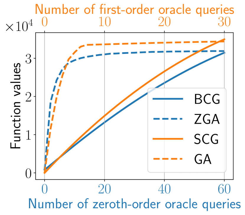
(a) NQP

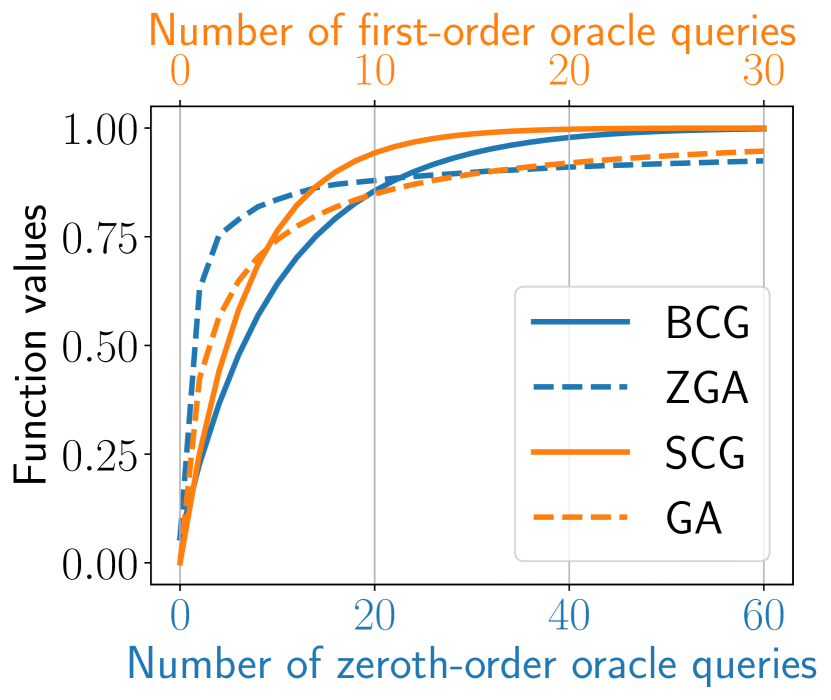
(b) Topic summarization

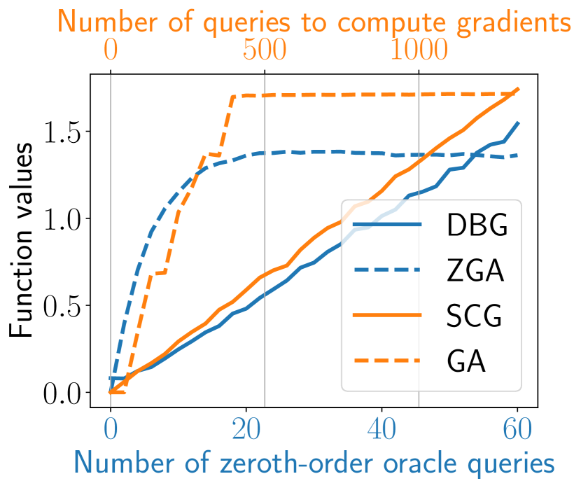
(c) Active set selection

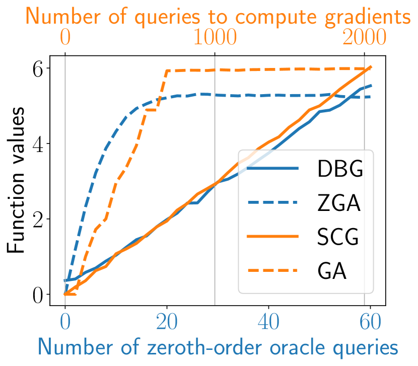
(d) Influence maximization

Figure 1: Function value vs. number of oracle queries. Note that every chart has dual horizontal axes. Orange lines use the orange horizontal axes above while blue lines use the blue ones below.

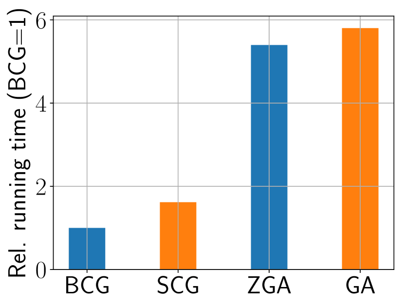
(a) NQP

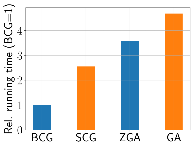
(b) Topic summarization

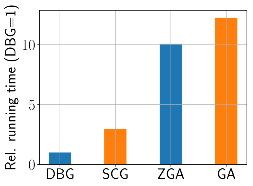
(c) Active set selection

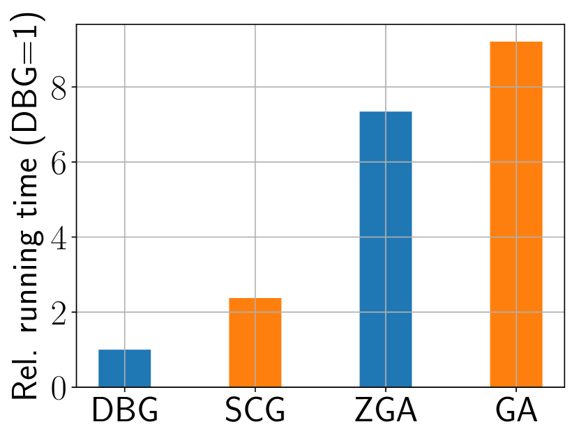
(d) Influence maximization

Figure 2: Relative running time normalized with respect to BCG (for continuous DR-submodular maximization in the first two sets of experiments) and DBG (for submodular set maximization in the last two sets of experiments).

Non-convex/non-concave Quadratic Programming (NQP): In this set of experiments, we apply our proposed algorithm and the baselines to the problem of non-convex/non-concave quadratic programming. The objective function is of the form $F(x)=\frac{1}{2}x^{\top}Hx+b^{\top}x$, where $x$ is a 100-dimensional vector, $H$ is a $100$-by-$100$ matrix, and every component of $H$ is an i.i.d. random variable whose distribution is equal to that of the negated absolute value of a standard normal distribution. The constraints are $\sum_{i=1}^{30}x_{i}\leq 30$, $\sum_{i=31}^{60}x_{i}\leq 20$, and $\sum_{i=61}^{100}x_{i}\leq 20$. To guarantee that the gradient is non-negative, we set $b_{t}=-H^{\top}\mathbf{1}$. One can observe from Fig. 1(a) that the function value that BCG attains is only slightly lower than that of the first-order algorithm SCG. The final function value that BCG attains is similar to that of ZGA.

Topic Summarization: Next, we consider the topic summarization problem (El-Arini et al., 2009; Yue and Guestrin, 2011), which is to maximize the probabilistic coverage of selected articles on news topics. Each news article is characterized by its topic distribution, which is obtained by applying latent Dirichlet allocation to the corpus of Reuters-21578, Distribution 1.0. The number of topics is set to 10. We will choose from 120 news articles. The probabilistic coverage of a subset of news articles (denoted by $X$) is defined by $f(X)=\frac{1}{10}\sum_{j=1}^{10}[1-\prod_{a\in X}(1-p_{a}(j))]$, where $p_{a}(\cdot)$ is the topic distribution of article $a$. The multilinear extension function of $f$ is $F(x)=\frac{1}{10}\sum_{j=1}^{10}[1-\prod_{a\in\Omega}(1-p_{a}(j)x_{a})]$, where $x\in[0,1]^{120}$ Iyer et al. (2014). The constraint is $\sum_{i=1}^{40}x_{i}\leq 25$, $\sum_{i=41}^{80}x_{i}\leq 30$, $\sum_{i=81}^{120}x_{i}\leq 35$. It can be observed from Fig. 1(b) that the proposed BCG algorithm achieves the same function value as the first-ordered algorithm SCG and outperforms the other two. As shown in Fig. 2(a), BCG is the most efficient method. The two projection-free algorithms BCG and SCG run faster than the projected methods ZGA and GA. We will elaborate on the running time later in this section.

Active Set Selection We study the active set selection problem that arises in Gaussian process regression Mirzasoleiman et al. (2013). We use the Parkinsons Telemonitoring dataset, which is composed of biomedical voice measurements from people with early-stage Parkinson’s disease (Tsanas et al., 2010). Let $\mathbf{X}\in\mathbb{R}^{n\times d}$ denote the data matrix. Each row $X[i,\mathrel{\mathop{\mathchar 58\relax}}]$ is a voice recording while each column $X[\mathrel{\mathop{\mathchar 58\relax}},j]$ denotes an attribute. The covariance matrix $\Sigma$ is defined by $\Sigma_{ij}=\exp(-\|X[\mathrel{\mathop{\mathchar 58\relax}},i]-X[\mathrel{\mathop{\mathchar 58\relax}},j]\|^{2})/h^{2}$, where $h$ is set to $0.75$. The objective function of the active set selection problem is defined by $f(S)=\log\det(I+\Sigma_{S,S})$, where $S\subseteq[d]$ and $\Sigma_{S,S}$ is the principal submatrix indexed by $S$. The total number of 22 attributes are partitioned into 5 disjoint subsets with sizes 4, 4, 4, 5 and 5, respectively. The problem is subject to a partition matroid requiring that at most one attribute should be active within each subset. Since this is a submodular set maximization problem, in order to evaluate the gradient (i.e., obtain an unbiased estimate of gradient) required by first-order algorithms SCG and GA, it needs $2d$ function value queries. To be precise, the $i$-th component of gradient is $\mathbb{E}_{S\sim x}[f(S\cup\{i\})-f(S)]$ and requires two function value queries. It can be observed from Fig. 1(c) that DBG outperforms the other zeroth-order algorithm ZGA. Although its performance is slightly worse than the two first-order algorithms SCG and GA, it require significantly less number of function value queries than the other two first-order methods (as discussed above).

Influence Maximization In the influence maximization problem, we assume that every node in the network is able to influence all of its one-hop neighbors. The objective of influence maximization is to select a subset of nodes in the network, called the seed set (and denoted by $S$), so that the total number of influenced nodes, including the seed nodes, is maximized. We choose the social network of Zachary’s karate club Zachary (1977) in this study. The subjects in this social network are partitioned into three disjoint groups, whose sizes are 10, 14, and 10 respectively. The chosen seed nodes should be subject to a partition matroid; i.e., We will select at most two subjects from each of the three groups. Note that this problem is also a submodular set maximization problem. Similar to the situation in the active set selection problem, first-order algorithms need function value queries to obtain an unbiased estimate of gradient. We can observe from Fig. 1(d) that DBG attains a better influence coverage than the other zeroth-order algorithm ZGA. Again, even though SCG and GA achieve a slightly better coverage, due to their first-order nature, they require a significantly larger number of function value queries.

Running Time

The running times of the our proposed algorithms and the baselines are presented in Fig. 2 for the above-mentioned experimental set-ups. There are two main conclusions. First, the two projection-based algorithms (ZGA and GA) require significantly higher time complexity compared to the projection-free algorithms (BCG, DBG, and SCG), as the projection-based algorithms require solving quadratic optimization problems whereas projection-free ones require solving linear optimization problems which can be solved more efficiently. Second, when we compare first-order and zeroth-order algorithms, we can observe that zeroth-order algorithms (BCG, DBG, and ZGA) run faster than their first-order counterparts (SCG and GA).

Summary

The above experiment results show the following major advantages of our method over the baselines including SCG and ZGA.

• BCG/DBG is at least twice faster than SCG and ZGA in all tasks in terms of running time (Figs. 2(a), 2(b), 2(c) and 2(d))

• DBG requires remarkably fewer function evaluations in the discrete setting (Figs. 1(c) and 1(d))

• In addition to saving function evaluations, BCG/DBG achieves an objective function value comparable to that of the first-order baselines SCG and GA.

Furthermore, we note that the number of first-order queries required by SCG is only half the number required by BCG. However, as is shown in Figs. 2(a) and 2(b), BCG runs significantly faster than SCG since a zeroth-order evaluation is faster than a first-order one.

In the topic summarization task (Fig. 1(b)), BCG exhibits a similar performance to that of the first-order baselines SCG and GA, in terms of the attained objective function value. In the other three tasks, BCG/DBG runs notably faster while achieving an only slightly inferior function value. Therefore, BCG/DBG is particularly preferable in a large-scale machine learning task and an application where the total number of function evaluations or the running time is subject to a budget.

6 Conclusion

In this paper, we presented Black-box Continuous Greedy, a derivative-free and projection-free algorithm for maximizing a monotone and continuous DR-submodular function subject to a general convex body constraint. We showed that Black-box Continuous Greedy achieves the tight $[(1-1/e)OPT-\epsilon]$ approximation guarantee with $\mathcal{O}(d/\epsilon^{3})$ function evaluations. We then extended the algorithm to the stochastic continuous setting and the discrete submodular maximization problem. Our experiments on both synthetic and real data validated the performance of our proposed algorithms. In particular, we observed that Black-box Continuous Greedy practically achieves the same utility as Continuous Greedy while being way more efficient in terms of number of function evaluations.

Appendix A Proof of Lemma 1

Proof.

Using the assumption that $F$ is $G$-Lipschitz continuous, we have

$$|\tilde{F}(x)-\tilde{F}(y)|= |\mathbb{E}_{v\sim B^{d}}[F(x+\delta v)-F(y+\delta v)]|$$ (15)

$$\leq \mathbb{E}_{v\sim B^{d}}[|F(x+\delta v)-F(y+\delta v)|]$$ (16)

$$\leq \mathbb{E}_{v\sim B^{d}}[G\|(x+\delta v)-(y+\delta v)\|]$$ (17)

$$= G\|x-y\|,$$ (18)

and

$$|\tilde{F}(x)-F(x)|= |\mathbb{E}_{v\sim B^{d}}[F(x+\delta v)-F(x)]|$$ (19)

$$\leq \mathbb{E}_{v\sim B^{d}}[|F(x+\delta v)-F(x)|]$$ (20)

$$\leq \mathbb{E}_{v\sim B^{d}}[G\delta\|v\|]$$ (21)

$$\leq \delta G.$$ (22)

If $F$ is $G$-Lipschitz continuous and monotone continuous DR-submodular, then $F$ is differentiable. For $\forall x\leq y$, we also have

$$\nabla F(x)\geq\nabla F(y),$$ (23)

and

$$F(x)\leq F(y).$$ (24)

By definition of $\tilde{F}$, we have $\tilde{F}$ is differentiable and for $\forall x\leq y$,

$$\nabla\tilde{F}(x)-\nabla\tilde{F}(y)= \nabla\mathbb{E}_{v\sim B^{d}}[F(x+\delta v)]-\nabla\mathbb{E}_{v\sim B^{d}}[F(y+\delta v)]$$ (25)

$$= \mathbb{E}_{v\sim B^{d}}[\nabla F(x+\delta v)-\nabla F(y+\delta v)]$$ (26)

$$\geq \mathbb{E}_{v\sim B^{d}}[0]$$ (27)

$$= 0,$$ (28)

and

$$\tilde{F}(x)-\tilde{F}(y)= \mathbb{E}_{v\sim B^{d}}[F(x+\delta v)]-\mathbb{E}_{v\sim B^{d}}[F(y+\delta v)]$$ (29)

$$= \mathbb{E}_{v\sim B^{d}}[F(x+\delta v)-F(y+\delta v)]$$ (30)

$$\leq \mathbb{E}_{v\sim B^{d}}[0]$$ (31)

$$= 0,$$ (32)

i.e., $\nabla\tilde{F}(x)\geq\nabla\tilde{F}(y),\tilde{F}(x)\leq\tilde{F}(y).$ So $\tilde{F}$ is also a monotone continuous DR-submodular function. ∎

Appendix B Proof of Theorem 1

In order to prove Theorem 1, we need the following variance reduction lemmas [Shamir, 2017, Chen et al., 2018b], where the second one is a slight improvement of Lemma 2 in [Mokhtari et al., 2018a] and Lemma 5 in [Mokhtari et al., 2018b].

Lemma 4 (Lemma 10 of [Shamir, 2017]).

It holds that

$$\mathbb{E}_{u\sim S^{d-1}}[\frac{d}{2\delta}(F(z+\delta u)-F(z-\delta u))u|z]=\nabla\tilde{F}(z),$$ (33)

$$\mathbb{E}_{u\sim S^{d-1}}[\|\frac{d}{2\delta}(F(z+\delta u)-F(z-\delta u))u-\nabla\tilde{F}(z)\|^{2}|z]\leq cdG^{2},$$ (34)

where $c$ is a constant.

Lemma 5 (Theorem 3 of [Chen et al., 2018b]).

Let $\{a_{t}\}_{t=0}^{T}$ be a sequence of points in $\mathbb{R}^{n}$ such that $\|a_{t}-a_{t-1}\|\leq G_{0}/(t+s)$ for all $1\leq t\leq T$ with fixed constants $G_{0}\geq 0$ and $s\geq 3$. Let $\{\tilde{a}_{t}\}_{t=1}^{T}$ be a sequence of random variables such that $\mathbb{E}[\tilde{a}_{t}|\mathcal{F}_{t-1}]=a_{t}$ and $\mathbb{E}[\|\tilde{a}_{t}-a_{t}\|^{2}|\mathcal{F}_{t-1}]\leq\sigma^{2}$ for every $t\geq 0$, where $\mathcal{F}_{t-1}$ is the $\sigma$-field generated by $\{\tilde{a}_{i}\}_{i=1}^{t}$ and $\mathcal{F}_{0}=\varnothing$. Let $\{d_{t}\}_{t=0}^{T}$ be a sequence of random variables where $d_{0}$ is fixed and subsequent $d_{t}$ are obtained by the recurrence

$$d_{t}=(1-\rho_{t})d_{t-1}+\rho_{t}\tilde{a}_{t}$$ (35)

with $\rho_{t}=\frac{2}{(t+s)^{2/3}}$. Then, we have

$$\mathbb{E}[\|a_{t}-d_{t}\|^{2}]\leq\frac{Q}{(t+s+1)^{2/3}},$$ (36)

where $Q\triangleq\max\{\|a_{0}-d_{0}\|^{2}(s+1)^{2/3},4\sigma^{2}+3G_{0}^{2}/2\}$.

Now we turn to prove Theorem 1.

Proof of Theorem 1.

First of all, we note that technically we need the iteration number $T\geq 4$, which always holds in practical applications.

Then we show that $\forall t=1,\dots,T+1$, $x_{t}\in\mathcal{D}_{\delta}$. By the definition of $x_{t}$, we have $x_{t}=\sum_{i=1}^{t-1}\frac{v_{i}}{T}$. Since $v_{t}$’s are non-negative vectors, we know that $x_{t}$’s are also non-negative vectors and that $0=x_{1}\leq x_{2}\leq\dots\leq x_{T+1}$. It suffices to show that $x_{T+1}\in\mathcal{D}_{\delta}$. Since $x_{T+1}$ is a convex combination of $v_{1},\dots,v_{T}$ and $v_{t}$’s are in $\mathcal{D}_{\delta}$, we conclude that $x_{T+1}\in\mathcal{D}_{\delta}$. In addition, since $v_{t}$’s are also in $\mathcal{K}-\delta\mathbf{1}$, $x_{T+1}$ is also in $\mathcal{K}-\delta\mathbf{1}$. Therefore our final choice $x_{T+1}+\delta\mathbf{1}$ resides in the constraint $\mathcal{K}$.

Let $z_{t}\triangleq x_{t}+\delta\mathbf{1}$ and the shrunk domain (without translation) $\mathcal{D}_{\delta}^{\prime}\triangleq\mathcal{D}_{\delta}+\delta\mathbf{1}=\prod_{i=1}^{d}[\delta,a_{i}-\delta]\subseteq\mathcal{D}$. By Jensen’s inequality and the fact $F$ has $L$-Lipschitz continuous gradients, we have

$$\|\nabla\tilde{F}(x)-\nabla\tilde{F}(y)\|\leq L\|x-y\|.$$ (37)

Thus,

$$\tilde{F}(z_{t+1})-\tilde{F}(z_{t})= \tilde{F}(z_{t}+\frac{v_{t}}{T})-\tilde{F}(z_{t})$$ (38)

$$\geq \frac{1}{T}\nabla\tilde{F}(z_{t})^{\top}v_{t}-\frac{L}{2T^{2}}\|v_{t}\|^{2}$$ (39)

$$\geq \frac{1}{T}\nabla\tilde{F}(z_{t})^{\top}v_{t}-\frac{L}{2T^{2}}D_{1}^{2}$$ (40)

$$= \frac{1}{T}\left(\bar{g}_{t}^{\top}v_{t}+(\nabla\tilde{F}(z_{t})-\bar{g}_{t})^{\top}v_{t}\right)-\frac{L}{2T^{2}}D_{1}^{2}.$$ (41)

Let $x^{*}_{\delta}\triangleq\operatorname*{arg\,max}_{x\in\mathcal{D}_{\delta}^{\prime}\cap\mathcal{K}}\tilde{F}(x)$. Since $x^{*}_{\delta},z_{t}\in\mathcal{D}_{\delta}^{\prime}$, we have $v_{t}^{*}\triangleq(x^{*}_{\delta}-z_{t})\vee 0\in\mathcal{D}_{\delta}$. We know $z_{t}+v_{t}^{*}=x_{\delta}^{*}\vee z_{t}\in\mathcal{D}_{\delta}^{\prime}$ and

$$v_{t}^{*}+\delta\mathbf{1}=(x_{\delta}^{*}-x_{t})\vee\delta\mathbf{1}\leq x_{\delta}^{*}.$$ (42)

Since we assume that $F$ is monotone continuous DR-submodular, by Lemma 1, $\tilde{F}$ is also monotone continuous DR-submodular. As a result, $\tilde{F}$ is concave along non-negative directions, and $\nabla\tilde{F}$ is entry-wise non-negative. Thus we have

$$\tilde{F}(z_{t}+v_{t}^{*})-\tilde{F}(z_{t})\leq \nabla\tilde{F}(z_{t})^{\top}v_{t}^{*}$$ (43)

$$\leq \nabla\tilde{F}(z_{t})^{\top}(x_{\delta}^{*}-\delta\mathbf{1}).$$ (44)

Since $x_{\delta}^{*}-\delta\mathbf{1}\in\mathcal{K}^{\prime}$, we deduce

$$\bar{g}_{t}^{\top}v_{t}\geq \bar{g}_{t}^{\top}(x_{\delta}^{*}-\delta\mathbf{1})$$ (45)

$$= \nabla\tilde{F}(z_{t})^{\top}(x_{\delta}^{*}-\delta\mathbf{1})+(\bar{g}_{t}-\nabla\tilde{F}(z_{t}))^{\top}(x_{\delta}^{*}-\delta\mathbf{1})$$ (46)

$$\geq \tilde{F}(z_{t}+v_{t}^{*})-\tilde{F}(z_{t})+(\bar{g}_{t}-\nabla\tilde{F}(z_{t}))^{\top}(x_{\delta}^{*}-\delta\mathbf{1})$$ (47)

$$\geq \tilde{F}(x_{\delta}^{*})-\tilde{F}(z_{t})+(\bar{g}_{t}-\nabla\tilde{F}(z_{t}))^{\top}(x_{\delta}^{*}-\delta\mathbf{1}).$$ (48)

Therefore, we obtain

$$\bar{g}_{t}^{\top}v_{t}+(\nabla\tilde{F}(z_{t})-\bar{g}_{t})^{\top}v_{t}\geq\tilde{F}(x_{\delta}^{*})-\tilde{F}(z_{t})+(\nabla\tilde{F}(z_{t})-\bar{g}_{t})^{\top}(v_{t}-(x_{\delta}^{*}-\delta\mathbf{1})).$$ (49)

By plugging Eq. 49 into Eq. 41, after re-arrangement of the terms, we obtain

$$h_{t+1}\leq(1-\frac{1}{T})h_{t}+\frac{1}{T}(\nabla\tilde{F}(z_{t})-\bar{g}_{t})^{\top}((x_{\delta}^{*}-\delta\mathbf{1})-v_{t})+\frac{L}{2T^{2}}D_{1}^{2},$$ (50)

where $h_{t}\triangleq\tilde{F}(x_{\delta}^{*})-\tilde{F}(z_{t})$. Next we derive an upper bound for $(\nabla\tilde{F}(z_{t})-\bar{g}_{t})^{\top}((x_{\delta}^{*}-\delta\mathbf{1})-v_{t})$. By Young’s inequality, it can be deduced that for any $\beta_{t}>0$,

$$(\nabla\tilde{F}(z_{t})-\bar{g}_{t})^{\top}((x_{\delta}^{*}-\delta\mathbf{1})-v_{t})\leq \frac{\beta_{t}}{2}\|\nabla\tilde{F}(z_{t})-\bar{g}_{t}\|^{2}+\frac{1}{2\beta_{t}}\|(x_{\delta}^{*}-\delta\mathbf{1})-v_{t}\|^{2}$$ (51)

$$\leq \frac{\beta_{t}}{2}\|\nabla\tilde{F}(z_{t})-\bar{g}_{t}\|^{2}+\frac{1}{2\beta_{t}}D_{1}^{2}.$$ (52)

Now let $\mathcal{F}_{1}\triangleq\varnothing$ and $\mathcal{F}_{t}$ be the $\sigma$-field generate by $\{\bar{g}_{1},\dots,\bar{g}_{t-1}\}$, then by Lemma 4, we have

$$\mathbb{E}[\frac{d}{2\delta}(F(y_{t,i}^{+})-F(y_{t,i}^{-}))u_{t,i}|\mathcal{F}_{t-1}]=\nabla\tilde{F}(z_{t}),$$ (53)

and

$$\mathbb{E}[\|\frac{d}{2\delta}(F(y_{t,i}^{+})-F(y_{t,i}^{-}))u_{t,i}-\nabla\tilde{F}(z_{t})\|^{2}|\mathcal{F}_{t-1}]\leq cdG^{2}.$$ (54)

Therefore,

$$\mathbb{E}[g_{t}|\mathcal{F}_{t-1}]= \mathbb{E}[\frac{1}{B_{t}}\sum_{i=1}^{B_{t}}\frac{d}{2\delta}(F(y_{t,i}^{+})-F(y_{t,i}^{-}))u_{t,i}|\mathcal{F}_{t-1}]$$ (55)

$$= \nabla\tilde{F}(z_{t}),$$ (56)

and

$$\mathbb{E}[\|g_{t}-\nabla\tilde{F}(z_{t})\|^{2}|\mathcal{F}_{t-1}]= \frac{1}{B_{t}^{2}}\sum_{i=1}^{B_{t}}\mathbb{E}[\|\frac{d}{2\delta}(F(y_{t,i}^{+})-F(y_{t,i}^{-}))u_{t,i}-\nabla\tilde{F}(z_{t})\|^{2}|\mathcal{F}_{t-1}]$$ (57)

$$\leq \frac{cdG^{2}}{B_{t}}.$$ (58)

By Jensen’s inequality and the assumption $F$ is $L$-smooth, we have

$$\|\nabla\tilde{F}(z_{t})-\nabla\tilde{F}(z_{t-1})\|\leq L\frac{D_{1}}{T}\leq\frac{2LD_{1}}{t+3}.$$ (59)

Then by Lemma 5 with $s=3,d_{t}=\bar{g}_{t},\forall t\geq 0,\tilde{a}_{t}=g_{t},a_{t}=\nabla\tilde{F}(z_{t}),\forall t\geq 1,a_{0}=\nabla\tilde{F}(z_{1}),G_{0}=2LD_{1}$, we have

$$\mathbb{E}[\|\nabla\tilde{F}(z_{t})-\bar{g}_{t}\|^{2}]\leq\frac{Q}{(t+4)^{2/3}},$$ (60)

where $Q\triangleq\max\{\|\nabla\tilde{F}(x_{1}+\delta\mathbf{1})\|^{2}4^{2/3},\frac{4cdG^{2}}{B_{t}}+6L^{2}D_{1}^{2}\}$. Note that by Lemma 1, we have $\|\nabla\tilde{F}(x)\|\leq G$, thus we can re-define $Q=\max\{4^{2/3}G^{2},\frac{4cdG^{2}}{B_{t}}+6L^{2}D_{1}^{2}\}$.

Using Eqs. 50, 52 and 60 and taking expectation, we obtain

$$\mathbb{E}[h_{t+1}]\leq(1-\frac{1}{T})\mathbb{E}[h_{t}]+\frac{1}{T}\left(\frac{\beta_{t}}{2}\cdot\frac{Q}{(t+4)^{2/3}}+\frac{D_{1}^{2}}{2\beta_{t}}\right)+\frac{L}{2T^{2}}D_{1}^{2}\leq(1-\frac{1}{T})\mathbb{E}[h_{t}]+\frac{D_{1}Q^{1/2}}{T(t+4)^{1/3}}+\frac{L}{2T^{2}}D_{1}^{2},$$ (61)

where we set $\beta_{t}=\frac{D_{1}(t+4)^{1/3}}{Q^{1/2}}$. Using the above inequality recursively, we have

$$\mathbb{E}[h_{T+1}]\leq (1-\frac{1}{T})^{T}(\tilde{F}(x_{\delta}^{*})-\tilde{F}(\delta\mathbf{1}))+\sum_{t=1}^{T}\frac{D_{1}Q^{1/2}}{T(t+4)^{1/3}}+\frac{L}{2T}D_{1}^{2}$$ (62)

$$\leq e^{-1}(\tilde{F}(x_{\delta}^{*})-\tilde{F}(\delta\mathbf{1}))+\frac{D_{1}Q^{1/2}}{T}\int_{0}^{T}\frac{\operatorname{d\!}x}{(x+4)^{1/3}}+\frac{L}{2T}D_{1}^{2}$$ (63)

$$\leq e^{-1}(\tilde{F}(x_{\delta}^{*})-\tilde{F}(\delta\mathbf{1}))+\frac{D_{1}Q^{1/2}}{T}\frac{3}{2}(T+4)^{2/3}+\frac{L}{2T}D_{1}^{2}$$ (64)

$$\leq e^{-1}(\tilde{F}(x_{\delta}^{*})-\tilde{F}(\delta\mathbf{1}))+\frac{D_{1}Q^{1/2}}{T}\frac{3}{2}(2T)^{2/3}+\frac{L}{2T}D_{1}^{2}$$ (65)

$$\leq e^{-1}(\tilde{F}(x_{\delta}^{*})-\tilde{F}(\delta\mathbf{1}))+\frac{3D_{1}Q^{1/2}}{T^{1/3}}+\frac{LD_{1}^{2}}{2T}.$$ (66)

By re-arranging the terms, we conclude

$$(1-\frac{1}{e})\tilde{F}(x_{\delta}^{*})-\mathbb{E}[\tilde{F}(z_{T+1})]\leq -e^{-1}\tilde{F}(\delta\mathbf{1})+\frac{3D_{1}Q^{1/2}}{T^{1/3}}+\frac{LD_{1}^{2}}{2T}$$ (67)

$$\leq \frac{3D_{1}Q^{1/2}}{T^{1/3}}+\frac{LD_{1}^{2}}{2T},$$ (68)

where the second inequality holds since the image of $F$ is in $\mathbb{R}_{+}$.

By Lemma 1, we have $\tilde{F}(z_{T+1})\leq F(z_{T+1})+\delta G$ and

$$\tilde{F}(x_{\delta}^{*})\geq\tilde{F}(x^{*})-\delta G\sqrt{d}\geq F(x^{*})-\delta G(\sqrt{d}+1).$$ (69)

Therefore,

$$(1-\frac{1}{e})F(x^{*})-\mathbb{E}[F(z_{T+1})]\leq\frac{3D_{1}Q^{1/2}}{T^{1/3}}+\frac{LD_{1}^{2}}{2T}+\delta G(1+(\sqrt{d}+1)(1-\frac{1}{e})).$$ (70)

∎

Appendix C Proof of Theorem 2

Proof.

By the unbiasedness of $\hat{F}$ and Lemma 4, we have

$$\mathbb{E}[\frac{d}{2\delta}(\hat{F}(y_{t,i}^{+})-\hat{F}(y_{t,i}^{-}))u_{t,i}|\mathcal{F}_{t-1}]= \mathbb{E}[\mathbb{E}[\frac{d}{2\delta}(\hat{F}(y_{t,i}^{+})-\hat{F}(y_{t,i}^{-}))u_{t,i}|\mathcal{F}_{t-1},u_{t,i}]|\mathcal{F}_{t-1}]$$ (71)

$$= \mathbb{E}[\frac{d}{2\delta}(F(y_{t,i}^{+})-F(y_{t,i}^{-}))u_{t,i}|\mathcal{F}_{t-1}]$$ (72)

$$= \nabla\tilde{F}(z_{t}),$$ (73)

where $z_{t}=x_{t}+\delta\mathbf{1}$, and

$$\mathbb{E}[\|\frac{d}{2\delta}(\hat{F}(y_{t,i}^{+})-\hat{F}(y_{t,i}^{-}))u_{t,i}-\nabla\tilde{F}(z_{t})\|^{2}|\mathcal{F}_{t-1}]$$ (74)

$$= \mathbb{E}[\mathbb{E}[\|\frac{d}{2\delta}(F(y_{t,i}^{+})-F(y_{t,i}^{-}))u_{t,i}-\nabla\tilde{F}(z_{t})$$ (75)

$$+\frac{d}{2\delta}(\hat{F}(y_{t,i}^{+})-F(y_{t,i}^{+}))u_{t,i}$$ (76)

$$-\frac{d}{2\delta}(\hat{F}(y_{t,i}^{-})-F(y_{t,i}^{-}))u_{t,i}\|^{2}|\mathcal{F}_{t-1},u_{t,i}]|\mathcal{F}_{t-1}]$$ (77)

$$= \mathbb{E}[\mathbb{E}[\|\frac{d}{2\delta}(F(y_{t,i}^{+})-F(y_{t,i}^{-}))u_{t,i}-\nabla\tilde{F}(z_{t})\|^{2}|\mathcal{F}_{t-1},u_{t,i}]|\mathcal{F}_{t-1}]$$ (78)

$$+\mathbb{E}[\mathbb{E}[\|\frac{d}{2\delta}(\hat{F}(y_{t,i}^{+})-F(y_{t,i}^{+}))u_{t,i}\|^{2}|\mathcal{F}_{t-1},u_{t,i}]|\mathcal{F}_{t-1}]$$ (79)

$$+\mathbb{E}[\mathbb{E}[\|\frac{d}{2\delta}(\hat{F}(y_{t,i}^{-})-F(y_{t,i}^{-}))u_{t,i}\|^{2}|\mathcal{F}_{t-1},u_{t,i}]|\mathcal{F}_{t-1}]$$ (80)

$$\leq \mathbb{E}[\|\frac{d}{2\delta}(F(y_{t,i}^{+})-F(y_{t,i}^{-}))u_{t,i}-\nabla\tilde{F}(z_{t})\|^{2}|\mathcal{F}_{t-1}]$$ (81)

$$+\frac{d^{2}}{4\delta^{2}}\mathbb{E}[\mathbb{E}[|\hat{F}(y_{t,i}^{+})-F(y_{t,i}^{+})|^{2}\cdot\|u_{t,i}\|^{2}|\mathcal{F}_{t-1},u_{t,i}]|\mathcal{F}_{t-1}]$$ (82)

$$+\frac{d^{2}}{4\delta^{2}}\mathbb{E}[\mathbb{E}[|\hat{F}(y_{t,i}^{-})-F(y_{t,i}^{-})|^{2}\cdot\|u_{t,i}\|^{2}|\mathcal{F}_{t-1},u_{t,i}]|\mathcal{F}_{t-1}]$$ (83)

$$\leq cdG^{2}+\frac{d^{2}}{4\delta^{2}}\sigma_{0}^{2}+\frac{d^{2}}{4\delta^{2}}\sigma_{0}^{2}$$ (84)

$$= cdG^{2}+\frac{d^{2}}{2\delta^{2}}\sigma_{0}^{2}.$$ (85)

Then we have

$$\mathbb{E}[g_{t}|\mathcal{F}_{t-1}]= \mathbb{E}[\frac{1}{B_{t}}\sum_{i=1}^{B_{t}}\frac{d}{2\delta}(\hat{F}(y_{t,i}^{+})-\hat{F}(y_{t,i}^{-}))u_{t,i}|\mathcal{F}_{t-1}]$$ (86)

$$= \nabla\tilde{F}(z_{t}),$$ (87)

and

$$\mathbb{E}[\|g_{t}-\nabla\tilde{F}(z_{t})\|^{2}|\mathcal{F}_{t-1}]= \frac{1}{B_{t}^{2}}\sum_{i=1}^{B_{t}}\mathbb{E}[\|\frac{d}{2\delta}(\hat{F}(y_{t,i}^{+})-\hat{F}(y_{t,i}^{-}))u_{t,i}-\nabla\tilde{F}(z_{t})\|^{2}|\mathcal{F}_{t-1}]$$ (88)

$$\leq \frac{cdG^{2}+\frac{d^{2}}{2\delta^{2}}\sigma_{0}^{2}}{B_{t}}.$$ (89)

Similar to the proof of Theorem 1, we have

$$\mathbb{E}[\|\nabla\tilde{F}(z_{t})-\bar{g}_{t}\|^{2}]\leq\frac{Q}{(t+4)^{2/3}},$$ (90)

where $Q=\max\{4^{2/3}G^{2},6L^{2}D_{1}^{2}+\frac{4cdG^{2}+2d^{2}\sigma_{0}^{2}/\delta^{2}}{B_{t}}\}$. Thus we conclude

$$(1-\frac{1}{e})F(x^{*})-\mathbb{E}[F(z_{T+1})]\leq\frac{3D_{1}Q^{1/2}}{T^{1/3}}+\frac{LD_{1}^{2}}{2T}+\delta G(1+(\sqrt{d}+1)(1-\frac{1}{e})).$$ (91)

∎

Appendix D Proof of Lemma 3

Proof.

Recall that $F(x)=\mathbb{E}_{X\sim x}[f(X)]=\sum_{S\subseteq\Omega}f(S)\prod_{i\in S}x_{i}\prod_{j\notin S}(1-x_{j})$, then for any fixed $i\in[d]$, where $d=|\Omega|$, we have

$$|\frac{\partial F(x)}{\partial x_{i}}|= |\sum_{\begin{subarray}{c}S\subseteq\Omega\\ i\in S\end{subarray}}f(S)\prod_{\begin{subarray}{c}j\in S\\ j\neq i\end{subarray}}x_{j}\prod_{\begin{subarray}{c}k\notin S\\ k\neq i\end{subarray}}(1-x_{k})-\sum_{\begin{subarray}{c}S\subseteq\Omega\\ i\notin S\end{subarray}}f(S)\prod_{\begin{subarray}{c}j\in S\\ j\neq i\end{subarray}}x_{j}\prod_{\begin{subarray}{c}k\notin S\\ k\neq i\end{subarray}}(1-x_{k})|$$ (92)

$$\leq M[\sum_{\begin{subarray}{c}S\subseteq\Omega\\ i\in S\end{subarray}}\prod_{\begin{subarray}{c}j\in S\\ j\neq i\end{subarray}}x_{j}\prod_{\begin{subarray}{c}k\notin S\\ k\neq i\end{subarray}}(1-x_{k})+\sum_{\begin{subarray}{c}S\subseteq\Omega\\ i\notin S\end{subarray}}\prod_{\begin{subarray}{c}j\in S\\ j\neq i\end{subarray}}x_{j}\prod_{\begin{subarray}{c}k\notin S\\ k\neq i\end{subarray}}(1-x_{k})]$$ (93)

$$= 2M.$$ (94)

So we have

$$\|\nabla F(x)\|\leq 2M\sqrt{d}.$$ (95)

Then $F$ is $2M\sqrt{d}$-Lipschitz.

Now we turn to prove that $F$ has Lipschitz continuous gradients. Thanks to the multilinearity, we have

$$\frac{\partial F}{\partial x_{i}}=F(x|x_{i}=1)-F(x|x_{i}=0).$$ (96)

Since

$$F(x|x_{i}=1)=\sum_{\begin{subarray}{c}S\subseteq\Omega\\ i\in S\end{subarray}}f(S)\prod_{\begin{subarray}{c}j\in S\\ j\neq i\end{subarray}}x_{j}\prod_{\begin{subarray}{c}k\notin S\\ k\neq i\end{subarray}}(1-x_{k}),$$ (97)

we have

$$\frac{\partial F(x|x_{i}=1)}{\partial x_{i}}=0,$$ (98)

and for any fixed $j\neq i$,

$$|\frac{\partial F(x|x_{i}=1)}{\partial x_{j}}|= |\sum_{\begin{subarray}{c}S\subseteq\Omega\\ i,j\in S\end{subarray}}f(S)\prod_{\begin{subarray}{c}l\in S\\ l\notin\{i,j\}\end{subarray}}x_{l}\prod_{\begin{subarray}{c}k\notin S\\ k\notin\{i,j\}\end{subarray}}(1-x_{k})-\sum_{\begin{subarray}{c}S\subseteq\Omega\\ i\in S,j\notin S\end{subarray}}f(S)\prod_{\begin{subarray}{c}l\in S\\ l\notin\{i,j\}\end{subarray}}x_{l}\prod_{\begin{subarray}{c}k\notin S\\ k\notin\{i,j\}\end{subarray}}(1-x_{k})|$$ (99)

$$\leq M[\sum_{\begin{subarray}{c}S\subseteq\Omega\\ i,j\in S\end{subarray}}\prod_{\begin{subarray}{c}l\in S\\ l\notin\{i,j\}\end{subarray}}x_{l}\prod_{\begin{subarray}{c}k\notin S\\ k\notin\{i,j\}\end{subarray}}(1-x_{k})+\sum_{\begin{subarray}{c}S\subseteq\Omega\\ i\in S,j\notin S\end{subarray}}\prod_{\begin{subarray}{c}l\in S\\ l\notin\{i,j\}\end{subarray}}x_{l}\prod_{\begin{subarray}{c}k\notin S\\ k\notin\{i,j\}\end{subarray}}(1-x_{k})]$$ (100)

$$= 2M.$$ (101)

Similarly, we have $\frac{\partial F(x|x_{i}=0)}{\partial x_{i}}=0$, and $|\frac{\partial F(x|x_{i}=0)}{\partial x_{j}}|\leq 2M$ for $j\neq i$. So we conclude that

$$|\frac{\partial^{2}F}{\partial x_{j}\partial x_{i}}|\leq\begin{cases}0,&\quad\text{if }j=i,\\ 4M,&\quad\text{if }j\neq i.\end{cases}$$ (102)

Then $\|\nabla\frac{\partial F}{\partial x_{i}}\|\leq 4M\sqrt{d-1}$, i.e., $\frac{\partial F}{\partial x_{i}}$ is $4M\sqrt{d-1}$-Lipschitz.

Then we deduce that

$$\|\nabla F(z_{1})-\nabla F(z_{2})\|= \left[\sum_{i=1}^{d}\left(\frac{\partial F(z_{1})}{\partial x_{i}}-\frac{\partial F(z_{2})}{\partial x_{i}}\right)^{2}\right]^{1/2}$$ (103)

$$\leq \left[\sum_{i=1}^{d}(4M\sqrt{d-1})^{2}\|z_{1}-z_{2}\|^{2}\right]^{1/2}$$ (104)

$$= \sqrt{\sum_{i=1}^{d}(4M\sqrt{d-1})^{2}}\cdot\|z_{1}-z_{2}\|$$ (105)

$$= 4M\sqrt{d(d-1)}\|z_{1}-z_{2}\|.$$ (106)

So $F$ is $4M\sqrt{d(d-1)}$-smooth. ∎

Appendix E Proof of Theorem 3

Proof.

Recall that we define $z_{t}=x_{t}+\delta\mathbf{1}$. Then we have

$$\mathbb{E}[\|g_{t}-\nabla\tilde{F}(z_{t})\|^{2}|\mathcal{F}_{t-1}]= \frac{1}{B_{t}^{2}}\sum_{i=1}^{B_{t}}\mathbb{E}[\|\frac{d}{2\delta}(\bar{f}_{t,i}^{+}-\bar{f}_{t,i}^{-})u_{t,i}-\nabla\tilde{F}(z_{t})\|^{2}|\mathcal{F}_{t-1}]$$ (107)

$$= \frac{1}{B_{t}^{2}}\sum_{i=1}^{B_{t}}\mathbb{E}[\|[\frac{d}{2\delta}(F(y_{t,i}^{+})-F(y_{t,i}^{-}))u_{t,i}-\nabla\tilde{F}(z_{t})]$$ (108)

$$\quad+\frac{d}{2\delta}[\bar{f}_{t,i}^{+}-F(y_{t,i}^{+})]u_{t,i}-\frac{d}{2\delta}[\bar{f}_{t,i}^{-}-F(y_{t,i}^{-})]u_{t,i}\|^{2}|\mathcal{F}_{t-1}]$$ (109)

$$= \frac{1}{B_{t}^{2}}\sum_{i=1}^{B_{t}}\mathbb{E}[\|[\frac{d}{2\delta}(F(y_{t,i}^{+})-F(y_{t,i}^{-}))u_{t,i}-\nabla\tilde{F}(z_{t})]\|^{2}|\mathcal{F}_{t-1}]$$ (110)

$$\quad+\frac{1}{B_{t}^{2}}\sum_{i=1}^{B_{t}}\mathbb{E}[|\frac{d}{2\delta}[\bar{f}_{t,i}^{+}-F(y_{t,i}^{+})]|^{2}|\mathcal{F}_{t-1}]$$ (111)

$$\quad+\frac{1}{B_{t}^{2}}\sum_{i=1}^{B_{t}}\mathbb{E}[|\frac{d}{2\delta}[\bar{f}_{t,i}^{-}-F(y_{t,i}^{-})]|^{2}|\mathcal{F}_{t-1}],$$ (112)

where we used the independence of $\bar{f}^{\pm}_{t,i}$ and the facts that $\mathbb{E}[\bar{f}^{\pm}_{t,i}]=F(y^{\pm}_{t,i}),\mathbb{E}[\frac{d}{2\delta}(F(y_{t,i}^{+})-F(y_{t,i}^{-}))u_{t,i}]=\nabla\tilde{F}(z_{t})$.

Then same to Eq. 58 and by Lemma 3, the first item is no more than $\frac{4cd^{2}M^{2}}{B_{t}}$. To upper bound the last two items, we have for every $i\in[B_{t}]$,

$$\begin{split}\mathbb{E}[|\frac{d}{2\delta}[\bar{f}_{t,i}^{+}-F(y_{t,i}^{+})]|^{2}|\mathcal{F}_{t-1}]&=\frac{d^{2}}{4\delta^{2}}\mathbb{E}[[\sum_{j=1}^{l}[f(Y_{t,i,j}^{+})-F(y_{t,i}^{+})]/l]^{2}|\mathcal{F}_{t-1}]\\ &\leq\frac{d^{2}}{4\delta^{2}}\cdot l\cdot\frac{M^{2}}{l^{2}}\\ &=\frac{d^{2}M^{2}}{4l\delta^{2}}.\end{split}$$ (113)

Similarly, we have

$$\mathbb{E}[|\frac{d}{2\delta}[\bar{f}_{t,i}^{-}-F(y_{t,i}^{-})]|^{2}|\mathcal{F}_{t-1}]\leq\frac{d^{2}M^{2}}{4l\delta^{2}}.$$ (114)

As a result, we have

$$\begin{split}\mathbb{E}[\|g_{t}-\nabla\tilde{F}(z_{t})\|^{2}|\mathcal{F}_{t-1}]&\leq\frac{4cd^{2}M^{2}}{B_{t}}+\frac{1}{B_{t}^{2}}\cdot B_{t}\cdot\frac{d^{2}M^{2}}{4l\delta^{2}}+\frac{1}{B_{t}^{2}}\cdot B_{t}\cdot\frac{d^{2}M^{2}}{4l\delta^{2}}\\ &=\frac{4cd^{2}M^{2}}{B_{t}}+\frac{d^{2}M^{2}}{2B_{t}l\delta^{2}}.\end{split}$$ (115)

Then same to the proof for Theorem 1, we have

$$(1-\frac{1}{e})F(x^{*})-\mathbb{E}[F(z_{T+1})]\leq\frac{3D_{1}Q^{1/2}}{T^{1/3}}+\frac{2M\sqrt{d(d-1)}D_{1}^{2}}{T}+2M\delta\sqrt{d}(1+(\sqrt{d}+1)(1-\frac{1}{e})).$$ (116)

where $D_{1}\triangleq\operatorname*{diam}(\mathcal{K}^{\prime})$, $Q=\max\{4^{5/3}dM^{2},\frac{2d^{2}M^{2}(8c+\frac{1}{l\delta^{2}})}{B_{t}}+96d(d-1)M^{2}D_{1}^{2}\}$, $x^{*}$ is the global maximizer of $F$ on $\mathcal{K}$.

Note that since the rounding scheme is lossless, we have

$$(1-\frac{1}{e})f(X^{*})-\mathbb{E}[f(X_{T+1})]\leq(1-\frac{1}{e})F(x^{*})-\mathbb{E}[F(z_{T+1})].$$ (117)

Combine Eqs. 117 and 116, we have

$$(1-\frac{1}{e})f(X^{*})-\mathbb{E}[f(X_{T+1})]\leq\frac{3D_{1}Q^{1/2}}{T^{1/3}}+\frac{2M\sqrt{d(d-1)}D_{1}^{2}}{T}+2M\delta\sqrt{d}(1+(\sqrt{d}+1)(1-\frac{1}{e})).$$ (118)

∎

References

- Agarwal et al. [2010] Alekh Agarwal, Ofer Dekel, and Lin Xiao. Optimal algorithms for online convex optimization with multi-point bandit feedback. In COLT, pages 28–40. Citeseer, 2010.
- Ageev and Sviridenko [2004] Alexander A Ageev and Maxim I Sviridenko. Pipage rounding: A new method of constructing algorithms with proven performance guarantee. Journal of Combinatorial Optimization, 8(3):307–328, 2004.
- Audet and Hare [2017] Charles Audet and Warren Hare. Derivative-free and blackbox optimization. Springer, 2017.
- Bach [2016] Francis Bach. Submodular functions: from discrete to continuous domains. Mathematical Programming, pages 1–41, 2016.
- Bach et al. [2012] Francis Bach, Rodolphe Jenatton, Julien Mairal, Guillaume Obozinski, et al. Optimization with sparsity-inducing penalties. Foundations and Trends® in Machine Learning, 4(1):1–106, 2012.
- Bach [2010] Francis R Bach. Structured sparsity-inducing norms through submodular functions. In Advances in Neural Information Processing Systems, pages 118–126, 2010.
- Balasubramanian and Ghadimi [2018] Krishnakumar Balasubramanian and Saeed Ghadimi. Zeroth-order (non)-convex stochastic optimization via conditional gradient and gradient updates. In Advances in Neural Information Processing Systems, pages 3459–3468, 2018.
- Balkanski and Singer [2015] Eric Balkanski and Yaron Singer. Mechanisms for fair attribution. In Proceedings of the Sixteenth ACM Conference on Economics and Computation, pages 529–546. ACM, 2015.
- Bateni et al. [2019] Mohammadhossein Bateni, Lin Chen, Hossein Esfandiari, Thomas Fu, Vahab Mirrokni, and Afshin Rostamizadeh. Categorical feature compression via submodular optimization. In International Conference on Machine Learning, pages 515–523, 2019.
- Bergstra et al. [2011] James S Bergstra, Rémi Bardenet, Yoshua Bengio, and Balázs Kégl. Algorithms for hyper-parameter optimization. In Advances in neural information processing systems, pages 2546–2554, 2011.
- Bian et al. [2017a] An Bian, Kfir Levy, Andreas Krause, and Joachim M Buhmann. Continuous dr-submodular maximization: Structure and algorithms. In Advances in Neural Information Processing Systems, pages 486–496, 2017a.
- Bian et al. [2018] An Bian, Joachim M Buhmann, and Andreas Krause. Optimal dr-submodular maximization and applications to provable mean field inference. arXiv preprint arXiv:1805.07482, 2018.
- Bian et al. [2017b] Andrew An Bian, Baharan Mirzasoleiman, Joachim Buhmann, and Andreas Krause. Guaranteed non-convex optimization: Submodular maximization over continuous domains. In Artificial Intelligence and Statistics, pages 111–120, 2017b.
- Calinescu et al. [2011] Gruia Calinescu, Chandra Chekuri, Martin Pál, and Jan Vondrák. Maximizing a monotone submodular function subject to a matroid constraint. SIAM Journal on Computing, 40(6):1740–1766, 2011.
- Celis et al. [2016] L Elisa Celis, Amit Deshpande, Tarun Kathuria, and Nisheeth K Vishnoi. How to be fair and diverse? arXiv preprint arXiv:1610.07183, 2016.
- Chekuri et al. [2014] Chandra Chekuri, Jan Vondrák, and Rico Zenklusen. Submodular function maximization via the multilinear relaxation and contention resolution schemes. SIAM Journal on Computing, 43(6):1831–1879, 2014.
- Chen et al. [2017a] Lin Chen, Forrest W Crawford, and Amin Karbasi. Submodular variational inference for network reconstruction. In UAI, 2017a.
- Chen et al. [2017b] Lin Chen, Andreas Krause, and Amin Karbasi. Interactive submodular bandit. In NeurIPS, pages 141–152, 2017b.
- Chen et al. [2018a] Lin Chen, Moran Feldman, and Amin Karbasi. Weakly submodular maximization beyond cardinality constraints: Does randomization help greedy? In ICML, pages 804–813, 2018a.
- Chen et al. [2018b] Lin Chen, Christopher Harshaw, Hamed Hassani, and Amin Karbasi. Projection-free online optimization with stochastic gradient: From convexity to submodularity. In ICML, pages 813–822, 10–15 Jul 2018b.
- Chen et al. [2018c] Lin Chen, Hamed Hassani, and Amin Karbasi. Online continuous submodular maximization. In AISTATS, pages 1896–1905, 2018c.
- Chen et al. [2017c] Pin-Yu Chen, Huan Zhang, Yash Sharma, Jinfeng Yi, and Cho-Jui Hsieh. Zoo: Zeroth order optimization based black-box attacks to deep neural networks without training substitute models. In Proceedings of the 10th ACM Workshop on Artificial Intelligence and Security, pages 15–26. ACM, 2017c.
- Conn et al. [2009] Andrew R Conn, Katya Scheinberg, and Luis N Vicente. Introduction to derivative-free optimization, volume 8. Siam, 2009.
- Das and Kempe [2011] Abhimanyu Das and David Kempe. Submodular meets spectral: Greedy algorithms for subset selection, sparse approximation and dictionary selection. arXiv preprint arXiv:1102.3975, 2011.
- Eghbali and Fazel [2016] Reza Eghbali and Maryam Fazel. Designing smoothing functions for improved worst-case competitive ratio in online optimization. In Advances in Neural Information Processing Systems, pages 3287–3295, 2016.
- El-Arini et al. [2009] Khalid El-Arini, Gaurav Veda, Dafna Shahaf, and Carlos Guestrin. Turning down the noise in the blogosphere. In Proceedings of the 15th ACM SIGKDD international conference on Knowledge discovery and data mining, pages 289–298. ACM, 2009.
- Flaxman et al. [2005] Abraham D Flaxman, Adam Tauman Kalai, and H Brendan McMahan. Online convex optimization in the bandit setting: gradient descent without a gradient. In Proceedings of the sixteenth annual ACM-SIAM symposium on Discrete algorithms, pages 385–394. Society for Industrial and Applied Mathematics, 2005.
- Frank and Wolfe [1956] Marguerite Frank and Philip Wolfe. An algorithm for quadratic programming. Naval research logistics quarterly, 3(1-2):95–110, 1956.
- Ghadimi and Lan [2013] Saeed Ghadimi and Guanghui Lan. Stochastic first-and zeroth-order methods for nonconvex stochastic programming. SIAM Journal on Optimization, 23(4):2341–2368, 2013.
- Golovin and Krause [2011] Daniel Golovin and Andreas Krause. Adaptive submodularity: Theory and applications in active learning and stochastic optimization. Journal of Artificial Intelligence Research, 42:427–486, 2011.
- Guillory and Bilmes [2010] Andrew Guillory and Jeff Bilmes. Interactive submodular set cover. arXiv preprint arXiv:1002.3345, 2010.
- Hassani et al. [2017] Hamed Hassani, Mahdi Soltanolkotabi, and Amin Karbasi. Gradient methods for submodular maximization. In Advances in Neural Information Processing Systems, pages 5841–5851, 2017.
- Hassani et al. [2019] Hamed Hassani, Amin Karbasi, Aryan Mokhtari, and Zebang Shen. Stochastic continuous greedy++: When upper and lower bounds match. In Advances in Neural Information Processing Systems, pages 13066–13076, 2019.
- Hazan [2016] Elad Hazan. Introduction to online convex optimization. Foundations and Trends® in Optimization, 2(3-4):157–325, 2016.
- Hazan and Luo [2016] Elad Hazan and Haipeng Luo. Variance-reduced and projection-free stochastic optimization. In International Conference on Machine Learning, pages 1263–1271, 2016.
- Ilyas et al. [2018] Andrew Ilyas, Logan Engstrom, Anish Athalye, Jessy Lin, Anish Athalye, Logan Engstrom, Andrew Ilyas, and Kevin Kwok. Black-box adversarial attacks with limited queries and information. In Proceedings of the 35th International Conference on Machine Learning,ICML 2018, 2018.
- Iyer et al. [2014] Rishabh Iyer, Stefanie Jegelka, and Jeff Bilmes. Monotone closure of relaxed constraints in submodular optimization: Connections between minimization and maximization. In Uncertainty in Artificial Intelligence (UAI), Quebic City, Quebec Canada, July 2014. AUAI.
- Jaggi [2013] Martin Jaggi. Revisiting frank-wolfe: Projection-free sparse convex optimization. In ICML (1), pages 427–435, 2013.
- Jegelka and Bilmes [2011a] Stefanie Jegelka and Jeff Bilmes. Submodularity beyond submodular energies: coupling edges in graph cuts. 2011a.
- Jegelka and Bilmes [2011b] Stefanie Jegelka and Jeff A Bilmes. Approximation bounds for inference using cooperative cuts. In Proceedings of the 28th International Conference on Machine Learning (ICML-11), pages 577–584, 2011b.
- Kempe et al. [2003] David Kempe, Jon Kleinberg, and Éva Tardos. Maximizing the spread of influence through a social network. In Proceedings of the ninth ACM SIGKDD international conference on Knowledge discovery and data mining, pages 137–146. ACM, 2003.
- Kulesza et al. [2012] Alex Kulesza, Ben Taskar, et al. Determinantal point processes for machine learning. Foundations and Trends® in Machine Learning, 5(2–3):123–286, 2012.
- Lacoste-Julien and Jaggi [2015] Simon Lacoste-Julien and Martin Jaggi. On the global linear convergence of frank-wolfe optimization variants. In Advances in Neural Information Processing Systems, pages 496–504, 2015.
- Lei et al. [2019] Qi Lei, Lingfei Wu, Pin-Yu Chen, Alexandros Dimakis, Inderjit Dhillon, and Michael Witbrock. Discrete adversarial attacks and submodular optimization with applications to text classification. Systems and Machine Learning (SysML), 2019.
- Lin and Bilmes [2011a] Hui Lin and Jeff Bilmes. A class of submodular functions for document summarization. In Proceedings of the 49th Annual Meeting of the Association for Computational Linguistics: Human Language Technologies-Volume 1, pages 510–520. Association for Computational Linguistics, 2011a.
- Lin and Bilmes [2011b] Hui Lin and Jeff Bilmes. Word alignment via submodular maximization over matroids. In Proceedings of the 49th Annual Meeting of the Association for Computational Linguistics: Human Language Technologies: short papers-Volume 2, pages 170–175. Association for Computational Linguistics, 2011b.
- Mirzasoleiman et al. [2013] Baharan Mirzasoleiman, Amin Karbasi, Rik Sarkar, and Andreas Krause. Distributed submodular maximization: Identifying representative elements in massive data. In Advances in Neural Information Processing Systems, pages 2049–2057, 2013.
- Mokhtari et al. [2018a] Aryan Mokhtari, Hamed Hassani, and Amin Karbasi. Conditional gradient method for stochastic submodular maximization: Closing the gap. In AISTATS, pages 1886–1895, 2018a.
- Mokhtari et al. [2018b] Aryan Mokhtari, Hamed Hassani, and Amin Karbasi. Stochastic conditional gradient methods: From convex minimization to submodular maximization. arXiv preprint arXiv:1804.09554, 2018b.
- Nemhauser et al. [1978] George L Nemhauser, Laurence A Wolsey, and Marshall L Fisher. An analysis of approximations for maximizing submodular set functions—i. Mathematical programming, 14(1):265–294, 1978.
- Rios and Sahinidis [2013] Luis Miguel Rios and Nikolaos V Sahinidis. Derivative-free optimization: a review of algorithms and comparison of software implementations. Journal of Global Optimization, 56(3):1247–1293, 2013.
- Rodriguez and Schölkopf [2012] Manuel Gomez Rodriguez and Bernhard Schölkopf. Influence maximization in continuous time diffusion networks. arXiv preprint arXiv:1205.1682, 2012.
- Sahu et al. [2018] Anit Kumar Sahu, Manzil Zaheer, and Soummya Kar. Towards gradient free and projection free stochastic optimization. arXiv preprint arXiv:1810.03233, 2018.
- Salehi et al. [2017] Mehraveh Salehi, Amin Karbasi, Dustin Scheinost, and R Todd Constable. A submodular approach to create individualized parcellations of the human brain. In International Conference on Medical Image Computing and Computer-Assisted Intervention, pages 478–485. Springer, 2017.
- Shahriari et al. [2016] Bobak Shahriari, Kevin Swersky, Ziyu Wang, Ryan P Adams, and Nando De Freitas. Taking the human out of the loop: A review of bayesian optimization. Proceedings of the IEEE, 104(1):148–175, 2016.
- Shamir [2017] Ohad Shamir. An optimal algorithm for bandit and zero-order convex optimization with two-point feedback. Journal of Machine Learning Research, 18(52):1–11, 2017.
- Singla et al. [2014] Adish Singla, Ilija Bogunovic, Gábor Bartók, Amin Karbasi, and Andreas Krause. Near-optimally teaching the crowd to classify. In ICML, pages 154–162, 2014.
- Snoek et al. [2012] Jasper Snoek, Hugo Larochelle, and Ryan P Adams. Practical bayesian optimization of machine learning algorithms. In Advances in neural information processing systems, pages 2951–2959, 2012.
- Sokolov et al. [2016] Artem Sokolov, Julia Kreutzer, Stefan Riezler, and Christopher Lo. Stochastic structured prediction under bandit feedback. In Advances in Neural Information Processing Systems, pages 1489–1497, 2016.
- Staib and Jegelka [2017] Matthew Staib and Stefanie Jegelka. Robust budget allocation via continuous submodular functions. arXiv preprint arXiv:1702.08791, 2017.
- Steudel et al. [2010] Bastian Steudel, Dominik Janzing, and Bernhard Schölkopf. Causal markov condition for submodular information measures. arXiv preprint arXiv:1002.4020, 2010.
- Taskar et al. [2005] Ben Taskar, Vassil Chatalbashev, Daphne Koller, and Carlos Guestrin. Learning structured prediction models: A large margin approach. In Proceedings of the 22nd international conference on Machine learning, pages 896–903. ACM, 2005.
- Thornton et al. [2013] Chris Thornton, Frank Hutter, Holger H Hoos, and Kevin Leyton-Brown. Auto-weka: Combined selection and hyperparameter optimization of classification algorithms. In Proceedings of the 19th ACM SIGKDD international conference on Knowledge discovery and data mining, pages 847–855. ACM, 2013.
- Tsanas et al. [2010] Athanasios Tsanas, Max A Little, Patrick E McSharry, and Lorraine O Ramig. Enhanced classical dysphonia measures and sparse regression for telemonitoring of parkinson’s disease progression. In Acoustics Speech and Signal Processing (ICASSP), 2010 IEEE International Conference on, pages 594–597. IEEE, 2010.
- Tschiatschek et al. [2014] Sebastian Tschiatschek, Rishabh K Iyer, Haochen Wei, and Jeff A Bilmes. Learning mixtures of submodular functions for image collection summarization. In Advances in neural information processing systems, pages 1413–1421, 2014.
- Vondrák [2008] Jan Vondrák. Optimal approximation for the submodular welfare problem in the value oracle model. In Proceedings of the fortieth annual ACM symposium on Theory of computing, pages 67–74. ACM, 2008.
- Wainwright et al. [2008] Martin J Wainwright, Michael I Jordan, et al. Graphical models, exponential families, and variational inference. Foundations and Trends® in Machine Learning, 1(1–2):1–305, 2008.
- Wang et al. [2017] Yining Wang, Simon Du, Sivaraman Balakrishnan, and Aarti Singh. Stochastic zeroth-order optimization in high dimensions. arXiv preprint arXiv:1710.10551, 2017.
- Wei et al. [2015] Kai Wei, Rishabh Iyer, and Jeff Bilmes. Submodularity in data subset selection and active learning. In International Conference on Machine Learning, pages 1954–1963, 2015.
- Yue and Guestrin [2011] Yisong Yue and Carlos Guestrin. Linear submodular bandits and their application to diversified retrieval. In Advances in Neural Information Processing Systems, pages 2483–2491, 2011.
- Zachary [1977] Wayne W Zachary. An information flow model for conflict and fission in small groups. Journal of anthropological research, 33(4):452–473, 1977.
- Zhang et al. [2019a] Mingrui Zhang, Lin Chen, Hamed Hassani, and Amin Karbasi. Online continuous submodular maximization: From full-information to bandit feedback. In Advances in Neural Information Processing Systems, pages 9206–9217, 2019a.
- Zhang et al. [2019b] Mingrui Zhang, Zebang Shen, Aryan Mokhtari, Hamed Hassani, and Amin Karbasi. One sample stochastic frank-wolfe. arXiv preprint arXiv:1910.04322, 2019b.
- Zhang et al. [2016] Yuanxing Zhang, Yichong Bai, Lin Chen, Kaigui Bian, and Xiaoming Li. Influence maximization in messenger-based social networks. In GLOBECOM, pages 1–6. IEEE, 2016.
- Zhou and Spanos [2016] Yuxun Zhou and Costas J Spanos. Causal meets submodular: Subset selection with directed information. In Advances in Neural Information Processing Systems, pages 2649–2657, 2016.