Forward and backward comparative study of jet properties in $pp$ collisions at $\sqrt{s}$=7 TeV

Abstract

We propose a forward method, based on the PYTHIA6.4, to study theoretically the jet properties in the ultra-relativistic $pp$ collisions. In the forward method, the partonic initial states are first generated with PYTHIA6.4 and then hadronized in the Lund srting fragmentation regime, and finally hadronic jets are constructed from the created hadrons. Jet properties calculated in the forward method for $pp$ collisions at $\sqrt{s}$=7 TeV are comparable with the corresponding ones calculated with usual anti-$k_{t}$ algorithm (backward method) in the PYTHIA6.4. The comparison between the results in the backward and forward methods may bring benefit to the understanding of the partonic origin of jets in the backward method.

I Introduction

In the early stage of ultra-relativistic heavy ion collisions, the hard parton scatterings generate high transverse momentum partons which traverse the medium and then hadronize into sprays of particles called jets Connors . Jet studies play an important role in understanding the properties of the medium created in ultra-relativistic heavy-ion collisions Solana . The “jet-quenching” together with the “elliptic flow” reveal much essential characters of the strongly coupled quark-gluon plasma (sQGP) in the ultra-relativistic heavy ion collisions at RHIC rhic1 ; rhic2 ; rhic3 ; rhic4 and LHC ALICE1 ; CMS1 ; ATLAS1 energies. With the higher collision energy, higher luminosity, and better detectors for jet measurements, the LHC experiments are able to measure the jet properties more precisely. Recently, the ATLAS, CMS, and ALICE collaborations have published a series results of jet properties in the pp, p+Pb, and Pb+Pb collisions at LHC energies ATLAS2 ; ATLAS3 ; ATLAS4 ; ATLAS5 ; ATLAS6 ; ALICE2 ; CMS2 ; CMS3 , where some new physics is arisen and needs to be studied urgently.

The perturbative Quantum Chromodynamics (pQCD) is able to describe the hard parton-parton scattering process and related initial and final state parton showers quantitatively. However, one can not apply the pQCD to directly describe the properties of particles within the jets, as the hadronization of partons is a non-perturbative process. To predict the intra-jet properties, phenomenological models may have to be employed. Several Monte Carlo (MC) event generators, like PYTHIA6.4 PYTHIA6.4 , PYTHIA8 PYTHIA8.2 , HERWIG HERWIG , HERWIG++ HERWIG++ , and SHERPA SHERPA etc., are available in the market. The results of MC event generators are sensitive to the model parameters assumed, which must be tuned to fit experimental data. In the end a number of PYTHIA tunes, such as Perugia 2011 tune Perugia etc., exist.

In the PYTHIA model, the Leading Order perturbative QCD (LO-pQCD) is used to generate the $2\rightarrow 2$ hard processes (parton-parton collisions). The parton shower model ps1 ; ps2 ; ps3 is employed to describe the initial and final state parton radiations. As for the soft processes (non-perturbative processes) several empirical options are availableunder1 ; under3 . Finally, the Lund string hadronization regime is used for the hadronization of partons string1 ; string2 ; string3 . In this work, the PYTHIA6.4 PYTHIA6.4 is employed to investigate the properties of particles in the jets in $pp$ collisions at $\sqrt{s}$=7 TeV using both the backward (usual anti-$k_{t}$ algorithm) and forward methods.

II Backward method for jet study

In the backward method we first employ PYTHIA6.4 to generate the final hadronic state for pp collisions at $\sqrt{s}$=7 TeV. Then the jet-finding algorithms, i.e. the anti-$k_{t}$ technique antik ; Salam , is used to backward reconstruct the jets as done in usual experimental jet analysis ATLAS3 . From the final hadronic state to the reconstructed hadronic jets, and to the searching for their partonic origin, this routine is opposite to the nature time evolution process of collisions, as sketched in the left part of Fig.(1). Hence it is referred to as backward method.

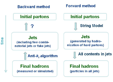
Figure 1: (color online) A sketch of backward method vs. forward method.

In the anti-$k_{t}$ algorithm, the distance $d_{ij}$ between entities (particle or energetic cluster) $i$ and $j$ is defined as antik :

$$d_{ij}={\rm min}(k^{-2}_{ti},k^{-2}_{tj})\frac{(\Delta R)^{2}_{ij}}{R^{2}},$$ (1)

where

$$(\Delta R)^{2}_{ij}=(y_{i}-y_{j})^{2}+(\phi_{i}-\phi_{j})^{2},$$ (2)

and $k_{ti}$, $y_{i}$ and $\phi_{i}$ are the transverse momentum, rapidity and azimuthal angle of particle $i$, respectively. The distance between particles $i$ and beam (B) $d_{iB}$ is defined as

$$d_{iB}=k^{-2}_{ti}.$$ (3)

With the distances $d_{ij}$ and $d_{iB}$, a list is compiled containing all the $d_{ij}$ and $d_{iB}$ for the particles in an event. If the smallest entry is a $d_{ij}$, particles $i$ and $j$ are combined (their four-vectors are added) as a jet. If the smallest entry is a $d_{iB}$, the particle $i$ is considered as a complete jet and removed from the list. The distances for all entities are recalculated and the procedure repeated until no entities are left. Thus the distance parameter $R$ in anti-$k_{t}$ algorithm is an essential quantity, within which the particles are reconstructed to a jet. If a hard particle has no hard neighbor within the distance 2$R$, then it will simply accumulate all the soft particles within a circle of radius $R$, resulting in a perfectly conical jet. If there is another hard particle $2$ in the area of $R<\Delta R_{12}<2R$, then there will be two jets. The shape of jet $1$ will be conical and jet $2$ will be partly conical when $k_{t1}\gg k_{t2}$; or both cones will be clipped when $k_{t1}\sim k_{t2}$ antik . The anti-$k_{t}$ algorithm is infrared and collinear safe and produces geometrically “conelike” jets, so it is widely used for jet reconstruction in experimental data analysis ATLAS2 ; ALICE2 ; CMS2 . The jets are reconstructed from the final hadronic state and hopefully to be attributed to the initial partonic state.

Based on the hadronic final states of $pp$ collisions at $\sqrt{s}$=7 TeV generated by the PYTHIA6.4, we use the anti-$k_{t}$ algorithm to reconstruct the jets. Following ATLAS ATLAS3 the charged particles with transverse momentum $p_{T}>$ 300 MeV/c and pseudorapidity $|\eta|<2.5$ are counted and the distance parameter $R$=0.6 is used. After the jet reconstruction, the clusters with $p_{T}>$ 4 GeV/c and $|y|<$ 1.9 are accepted as the jets, including those with only one particle in the cluster. The jets are divided into five bins according to their transverse momentum $p_{\rm{T,jet}}$, namely 4-6, 6-10, 10-15, 15-24 and 24-40 GeV/c. The jets with $p_{T}>$ 40 GeV/c and the particles not belong to any jet are excluded in the calculations.

After jets have been reconstructed in the anti-$k_{t}$ algorithm, we calculate the intra-jet particle distributions ATLAS3 :

$$F(z,p_{\rm{T,jet}})\equiv\frac{1}{N_{jet}}\frac{dN_{ch}}{dz},$$

$$f(p_{T}^{rel},p_{\rm{T,jet}})\equiv\frac{1}{N_{jet}}\frac{dN_{ch}}{dp_{T}^{rel}},$$

$$\rho_{ch}(r,p_{\rm{T,jet}})\equiv\frac{1}{N_{jet}}\frac{dN_{ch}}{2\pi rdr}.$$ (4)

The $N_{ch}$ and $N_{jet}$ in Eq. (II) are respectively the charged particle and jet numbers in a given jet $p_{\rm{T,jet}}$ bin. The variable $z$ (known as the fragmentation variable)

$$z=\frac{\vec{p}_{ch}\cdot\vec{p}_{jet}}{|\vec{p}_{jet}|^{2}}$$ (5)

is defined for each charged particle in a jet, and the variable $r$ stands for the radial distance from the charged particle to the axis of its jet,

$$r=\sqrt{(\phi_{ch}-\phi_{jet})^{2}+(y_{ch}-y_{jet})^{2}},$$ (6)

and the variable $p_{T}^{rel}$ refers to the momentum of charged particles in a jet, transverse to the jet axis,

$$p_{T}^{rel}=\frac{|\vec{p}_{ch}\times\vec{p}_{jet}|}{|\vec{p}_{jet}|^{2}},$$ (7)

where $\vec{p}_{ch}$ and $\vec{p}_{jet}$ are the momentum of the charged particle and the jet, respectively.

III Forward method for jet study

Beside the backward method we propose a forward method for the theoretical study of the jet analysis. In the forward method, we first employ the PYTHIA6.4 PYTHIA6.4 with the hadronization switched off temporarily to generate the partonic initial state for the $pp$ collisions at $\sqrt{s}$=7 TeV. The partonic initial state is originally composed of simple (without gluons between two quark ends) strings and complex (with gluons between two quark ends) strings. The gluons are first removed from the complex strings. All the gluons are then split into quark pairs, and each quark pair is modeled as a simple string. Hence the partonic initial state of the $pp$ collision is finally composed of simple strings only.

Secondly, each simple string in the the partonic initial state is hadronized in the Lund string hadronization model (i. e. by the subroutine of PYSTRF in the PYTHIA 6.4) individually. The hadrons from the hadronization of a simple string are first cataloged into two groups (related to the two quark ends) according to their relative transverse momentum to the quark ends. The hadrons bearing momenta closer to the momentum of one end of the string are grouped together. For instance, a hadron is grouped as the candidate of the left quark end jet if its relative transverse momentum to the left quark end is less than its relative transverse momentum to the right quark end.

Thirdly, the candidate of a quark end jet is determined to be the constituent of the jet if its distance relative to this quark end satisfies Eqs. (1) and (2) ($R=0.6$) in the rapidity and azimuthal (y-$\phi$) phase space. Finally, two original quark ends of a simple string are thus developed into two hadronic jets, a two-to-two correspondence.

The routine in forward method is as follows: 1) We create the partonic initial state by PYTHIA. 2) The simple strings are then constructed. 3) Each simple string is hadronized individually by Lund string fragmentation regime. 4) Final hadrons from two quark ends in a simple string are constructed to two jets. 5) The final hadronic state is resulted eventually. The process is parallel to the natural time evolution of collisions, as sketched in right part of Fig.(1). Therefore it is referred to as forward method.

IV Results

To show the solidity of the forward method we first employ it to calculate the final state charged particle transverse momentum and pseudorapidity distributions in pp collisions at $\sqrt{s}$=7 TeV. The results are shown in Figure (2) as triangles up and compared with the CMS experimental data (solid squares) CMS . In the calculation the K factor, “multiplying the differential cross section for hard parton-parton processes” in the PYTHIA6.4, is tuned to 4 from the default value of 1.5. One sees in Figure (2) that both the theoretical transverse momentum distribution and pseudorapidity distributions agree well with the CMS data. This tuned K factor of 4 is applied to all the later calculations.

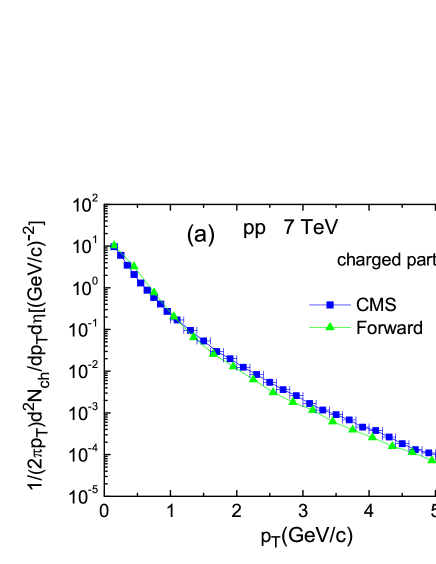
Figure 2: (color online) The transverse momentum (a) and pseudorapidity (b) distributions of final state charged particle in $pp$ collisions at $\sqrt{s}$=7 TeV calculated with forward method are compared with the CMS data (taken from Ref. CMS )

.

Then the intra-jet charged particle distributions of $F(z,p_{\rm{T,jet}})$, $f(p_{T}^{rel},p_{\rm{T,jet}})$ and $\rho_{ch}(r,p_{\rm{T,jet}})$ calculated in the backward method are compared with the corresponding ATLAS experimental data ATLAS3 (analyzed by anti-$k_{t}$ algorithm, i. e. by backward method) in Fig.(3a)-(3c) for the $pp$ collisions at $\sqrt{s}$ =7 TeV. We see in this figure that the theoretical results of the backward method fairly well agree with the ATLAS data except the theoretical results of $f(p_{T}^{rel},p_{\rm{T,jet}})$ is smaller than the ATLAS data at high $p_{T}^{rel}$ region for $p_{T,jet}$ bin of 10-15, 15-24 and 24-40.

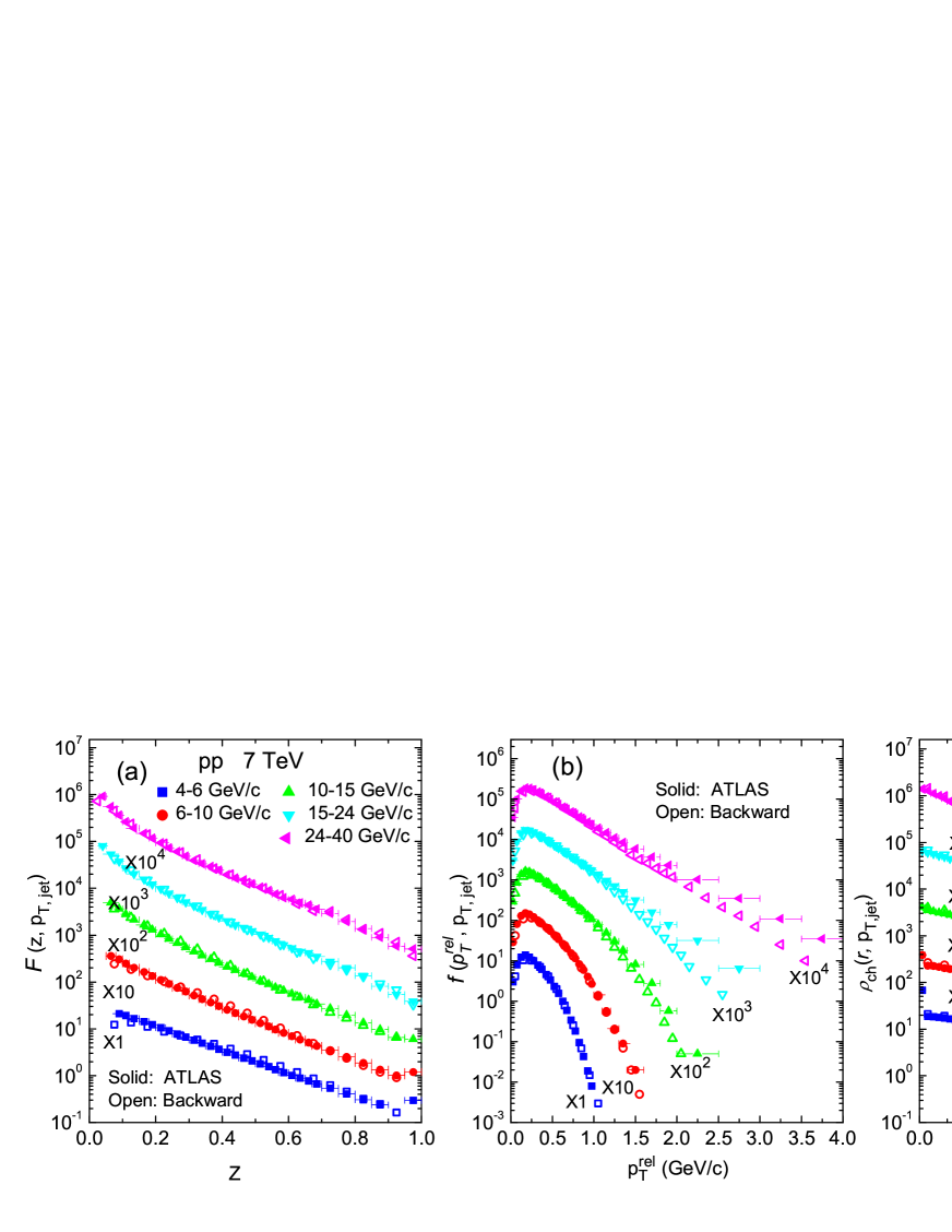
Figure 3: (color online) The intra-jet charged particle distributions of (a) $F(z,p_{\rm{T,jet}})$, (b) $f(p_{T}^{rel},p_{\rm{T,jet}})$ and (c) $\rho_{ch}(r,p_{\rm{T,jet}})$ in $p_{\rm{T,jet}}$ bins of 4-6, 6-10, 10-15, 15-24 and 24-40 GeV/c in $pp$ collisions at $\sqrt{s}$=7 TeV. The solid and open symbols are the ATLAS data ATLAS3 and results of backward method, respectively. The results in 6-10, 10-15, 15-24 and 24-40 GeV/c bins are multiplied by 10, $10^{2}$, $10^{3}$ and $10^{4}$, respectively. The distance parameter $R$=0.6 is assumed.

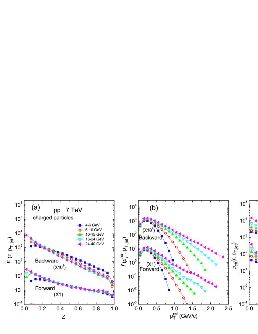
Figure 4: (color online) The intra-jet charged particle distributions of (a) $F(z,p_{\rm{T,jet}})$, (b) $f(p_{T}^{rel},p_{\rm{T,jet}})$ and (c) $\rho_{ch}(r,p_{\rm{T,jet}})$ calculated by forward method are compared to the ones calculated by backward methods for $p_{\rm{T,jet}}$ bins of 4-6, 6-10, 10-15, 15-24 and 24-40 GeV/c in $pp$ collisions at $\sqrt{s}$=7 TeV. The results of backward method are multiplied by $10^{2}$.

Furthermore, the intra-jet charged particle distributions of $F(z,p_{\rm{T,jet}})$, $f(p_{T}^{rel},p_{\rm{T,jet}})$ and $\rho_{ch}(r,p_{\rm{T,jet}})$ calculated in the forward method are compared with the ones calculated in the backward method in Fig.(4a)-(4c) for $pp$ collisions at $\sqrt{s}$=7 TeV. Fig. (4) shows that the results of the forward method are comparable with the backward method ones. We see the scaling phenomena in the $F(z,p_{T,jet})$ distributions for the high $p_{T,jet}$ bin of 10-15, 15-24 and 24-40 in backward methods and for all $p_{T,jet}$ bins in the forward method.

V Discussions and Conclusions

In this paper a forward method based on PYTHIA6.4 is proposed to study theoretically the properties of intra-jet charged particle distributions of $F(z,p_{\rm{T,jet}})$, $f(p_{T}^{rel},p_{\rm{T,jet}})$ and $\rho_{ch}(r,p_{\rm{T,jet}})$, and the calculated results are compared with ones calculated in backward method (usual anti-$k_{t}$ algorithm). The ATLAS data (analyzed with anti-$k_{t}$ algorithm) ATLAS3 of the intra-jet charged particle distributions of $F(z,p_{\rm{T,jet}})$ , $f(p_{T}^{rel},p_{\rm{T,jet}})$ and $\rho_{ch}(r,p_{\rm{T,jet}})$ in $pp$ collisions at $\sqrt{s}$=7 TeV are well reproduced in the backward method, as shown in Fig.(3). These distributions calculated in the forward method are comparable with the ones calculated in the backward method, as shown in Fig.(4a)-(4c).

By comparing the $F(z,p_{\rm{T,jet}})$, $f(p_{T}^{rel},p_{\rm{T,jet}})$ and $\rho_{ch}(r,p_{\rm{T,jet}})$ distributions resulted in the backward method to the ones resulted in the forward method, some light might shed on the problem of the correspondence between final hadronic jets and initial partons in the backward method. The forward method is possible to relate the final hadronic jet to its initial partonic origin, which helps to eliminate the effect from combinatorial jets or fake jets. The results of forward method can also serve a theoretical reference for the results of backward method in jet study. Of course, it has to be further studied.

As mentioned in Connors , one key problem of jet study in the backward method both experimentally and theoretically is to identify the jets which are really generated from hard scattered partons, and to eliminate the effect of combinatorial jets and fake jets. However, this problem does not exist in the forward method where the final hadronic jets are all constructed directly from the initial partonic strings. Therefore, the comparison between the $F(z,p_{\rm{T,jet}})$, $f(p_{T}^{rel},p_{\rm{T,jet}})$ and $\rho_{ch}(r,p_{\rm{T,jet}})$ distributions in the backward method and in the forward method may help to evaluate and/or to eliminate the effect of combinatorial jets and fake jets in the backward method. It needs to be further studied as well.

Acknowledgments This work was supported by the National Natural Science Foundation of China under grant Nos.: 11477130, 11775094 and by the 111 project of the foreign expert bureau of China. YLY, AL and YY acknowledge the financial support from Suranaree University of Technology and the Office of the Higher Education Commission under the NRU project of Thailand. YLY acknowledge the financial support from Key Laboratory of Quark and Lepton Physics in Central China Normal University under grant No. QLPL201805 and the Continuous Basic Scientific Research Project (No, WDJC-2019-13).

References

- (1) Megan Connors, Christine Nattrass, Rosi Reed, and Sevil Salur, Rev. Mod. Phys. 90, 025005 (2018).
- (2) J. Casalderrey-Solana and C. A. Salgado, Acta Phys. Polon. B 38 (2007) 3731.
- (3) I. Arsene, et al., BRAHMS Collaboration, Nucl. Phys. A 757 (2005) 1.
- (4) B. B. Back, et al.,PHOBOS Collaboration, Nucl. Phys. A 757 (2005) 28.
- (5) J. Admas, et al., STAR Collaboration, Nucl. Phys. A 757 (2005) 102.
- (6) K. Adcox, et al., PHENIX Collaboration, Nucl. Phys. A 757 (2005) 184.
- (7) K. Aamodt, et al., ALICE Collaboration, Phys. Lett. B 696 (2011) 30.
- (8) S. Chatrchyan, et al., CMS Collaboration, Eur. Phys. J. C 72 (2012) 1945.
- (9) G. Aad, et al., ATLAS Collaboration, Phys. Rev. C 86 (2012) 014907.
- (10) G. Aad, et al., ATLAS Collaboration, Phys. Rev. D 83 (2011) 052003.
- (11) G. Aad, et al., ATLAS Collaboration, Phys. Rev. D 84 (2011) 054001.
- (12) G. Aad, et al., ATLAS Collaboration, Eur. Phys. J. C 71 (2011) 1795.
- (13) G. Aad, et al., ATLAS Collaboration, Phys. Lett. B 739 (2014) 320.
- (14) M. Aaboud, et al., ATLAS Collaboration, CERN-EP-2017-065, arXiv:1706.02859.
- (15) R. Ma, ALICE Collaboration, Nucl. Phys. A 910-911 (2013) 319.
- (16) S. Chatrchyan, et al., CMS Collaboration, Phys. Rev. C 90 (2014) 024908.
- (17) S. Chatrchyan, et al., CMS Collaboration, J. High Energy Phys. 10 (2012) 087.
- (18) T. Sjöstrand, S. Mrenna, P. Skands, J. High Energy Phys., 05 (2006) 026, arXiv:hep-ph/0603175.
- (19) T. Sjöstrand, S. Ask, J. R. Christiansen, et al., Computer Physics Commun., 2015, 191: 159 C177.
- (20) G. Corcella, I.G. Knowles, G. Marchesini, S. Moretti, K. Odagiri, P. Richardson, M.H. Seymour and B.R. Webber, JHEP 0101 (2001) 010, arXiv:hep-ph/0011363.
- (21) M.Bähr et al., Eur. Phys. J. C58 (2008) 639, arXiv:0803.0883.
- (22) T. Gleisberg et al., JHEP 0902, 007 (2009), arXiv:hep-ph/0811.4622.
- (23) P. Z. Skands, Phys. Rev. D 82 (2010) 074018.
- (24) M. Bengtsson and T. Sjöstrand, Nucl. Phys. B 289 (1987) 810.
- (25) M. Bengtsson and T. Sjöstrand, Phys. Lett. B 185 (1987) 435.
- (26) T. Sjöstrand and P. Z. Skands, Eur. Phys. J. C 39 (2005) 129.
- (27) G.A. Schuler and T. Sjöstrand, Nucl. Phys. B 407 (1993) 539.
- (28) G.A. Schuler and T. Sjöstrand, Phys. Rev. D 49 (1994) 2257.
- (29) B. Andersson, G. Gustafson, G. Ingelman, and T. Sjöstrand, Phys. Rep. 97 (1983) 31.
- (30) B. Andersson, G. Gustafson, and B. Söderberg, Z. Phys. C 20 (1983) 317.
- (31) T. Sjöstrand, Nucl. Phys. B 248 (1984) 469.
- (32) M. Cacciari, G. P. Salam, and G. Soyez, J. High Energy Phys. 04 (2008) 063.
- (33) Gavin P. Salam, Eur. Phys. J. C 67 (2010) 637.
- (34) V. Khachatryan et al. (CMS Collaboration), Phys. Rev. Lett. 105 (2010) 022002.