Open clusters in APOGEE and GALAH

Abstract

Context. Open clusters are ideal laboratories to investigate a variety of astrophysical topics, from the properties of the Galactic disk to stellar evolutionary models. Knowing their metallicity and possibly detailed chemical abundances is therefore important. However, the number of systems with chemical abundances determined from high resolution spectroscopy is still small.

Aims. To increase the number of open clusters with radial velocities and chemical abundances determined from high resolution spectroscopy we used publicly available catalogues of surveys in combination with Gaia data.

Methods. Open cluster stars have been identified in the APOGEE and GALAH spectroscopic surveys by cross-matching their latest data releases with stars for which high-probability astrometric membership has been derived in many clusters on the basis of the Gaia second data release.

Results. Radial velocities have been determined for 131 and 14 clusters from APOGEE and GALAH data, respectively. This is the first radial velocity determination from high resolution spectra for 16 systems. Iron abundances have been obtained for 90 and 14 systems from APOGEE and GALAH samples, respectively. To our knowledge 66 of these clusters (57 in APOGEE and 9 in GALAH) do not have previous determinations in the literature. For 90 and 7 clusters in the APOGEE and GALAH samples, respectively, we have also determined average abundances for Na, Mg, Al, Si, Ca, Cr, Mn, and Ni.

1 Introduction

Open clusters (OCs) are groupings of between 10 and a few thousand stars that share chemo-dynamical features with a common birth-time and place. They are probably the only chemically homogeneous stellar populations (e.g. De Silva et al., 2007; Bovy, 2016) but see also Liu et al. (2016). These systems play a fundamental role in our understanding of both individual and group stellar evolution allowing to investigate a variety of astrophysical topics such as initial mass function, initial binary fraction, the creation of blue stragglers, mass loss, or atomic diffusion among others. Thanks to the fact that OCs cover a wide range of ages and are found everywhere in the Galactic disk, they have been widely used to trace both the disk chemistry, e.g. disk metallicity gradient (e.g. Friel et al., 2002; Donati et al., 2015a; Jacobson et al., 2016; Netopil et al., 2016; Casamiquela et al., 2017) and its evolution with time (e.g. Andreuzzi et al., 2011; Carrera & Pancino, 2011), and dynamics, e.g. individual orbits (e.g. Cantat-Gaudin et al., 2016; Reddy et al., 2016) or radial migration (e.g. Roškar et al., 2008; Anders et al., 2017).

A detailed characterisation of the OCs chemical composition is necessary to fully exploit their capabilities to address the topics described above. High-resolution spectroscopy ($R\geq$20,000) is the most direct way to obtain chemical abundances; however, for some OCs these studies have been limited to the determination of the iron content, widely known as metallicity. Moreover, this kind of analysis has been performed for slightly more than 100 objects (see e.g. the literature compilations by Carrera & Pancino, 2011; Yong et al., 2012; Heiter et al., 2014; Donati et al., 2015a; Netopil et al., 2016). They represent the 10% of the about 3000 known OCs according to the updated versions of the two most used OCs compilations by Dias et al. (2002, DAML) and Kharchenko et al. (2013, MWSC). The real cluster population is still largely unknown; not only many of these 3000 objects need to be confirmed as real clusters (see e.g. Kos et al., 2018b; Cantat-Gaudin et al., 2018, for objects that are likely not clusters), but new clusters are being discovered thanks to surveys like the Gaia mission (see later).

The Gaia mission (Gaia Collaboration et al., 2016) is carrying out a revolution in astronomy providing an unprecedented large volume of high quality positions, parallaxes and proper motions. This is supplemented by very high-accuracy all-sky photometric measurements. Additionally, for the brightest stars Gaia is also providing radial velocities (Sartoretti et al., 2018) and in the future it will provide some information about their chemical composition (Bailer-Jones et al., 2013).

Complementing the limited spectroscopic capabilities of Gaia is the motivation of the several ongoing and forthcoming ground-based high-resolution spectroscopic surveys providing radial velocities and chemical abundances for more than 20 chemical species. At the moment the Gaia-ESO Survey (GES Gilmore et al., 2012; Randich et al., 2013) is the only high-resolution survey which has dedicated a significant fraction of time to target open clusters. Gaia-ESO is providing an homogeneous set for about 80 clusters (see e.g. Jacobson et al., 2016; Randich et al., 2018, and references therein) observed extensively (100-1000 stars targeted in each of them). The other two high-resolution surveys with data published until now, APOGEE (Apache Point Observatory Galactic Evolution Experiment; Majewski et al., 2017) and GALAH (Galactic Archaeology with HERMES; De Silva et al., 2015), do not have such a large and specific program on OCs, although they are targeting some of them, also for calibration purposes (see e.g. Donor et al. 2018; Kos et al. 2018a). Their latest data releases include about 277,000 (Holtzman et al., 2018) and 340,000 (Buder et al., 2018) stars, respectively.

This paper is the third of a series devoted to the study of OCs on the basis of Gaia DR2. In the first one, membership probabilities for OCs were derived from the Gaia DR2 astrometric solutions (Cantat-Gaudin et al., 2018). In the second, the Gaia DR2 radial velocities were used to investigate the distribution of OCs in the 6D space (Soubiran et al., 2018). The goal of this paper is to search for cluster stars hidden in both the APOGEE and GALAH catalogues in order to increase the number of OCs with radial velocities and chemical abundances derived from high resolution spectroscopy. To do so, we use the astrometric membership probabilities obtained by Cantat-Gaudin et al. (2018).

This paper is organized as follows. The observational material utilized in the paper is described in Sect. 2. The radial velocities are discussed in Sect. 3. The iron and other elements abundances are presented in Sect. 4 and 5, respectively. An example of the usefulness of the results obtained in previous sections to investigate the radial and vertical chemical distribution of OCs in the Galactic disk is shown in Sect.6. Finally, the main conclusions of this paper are discussed in Sect. 7.

2 The Data

The Gaia DR2 provides 5-parameter astrometric solution (positions, proper motions $\mu_{\alpha*}$, $\mu_{\delta}$, and parallaxes $\varpi$; Lindegren et al., 2018) and magnitudes in three photometric bands ($G$, $G_{BP}$ and $G_{RP}$; Evans et al., 2018) for more than 1.3 billion sources (Gaia Collaboration et al., 2018), plus radial velocities (RV) for more than 7 million stars (Katz et al., 2018). On the basis of Gaia DR2, Cantat-Gaudin et al. (2018) determined membership probabilities for stars in 1229 OCs, 60 of which are new clusters serendipitously discovered in the fields analysed. Because of the large uncertainties of the proper motion and parallax determinations for faint objects, the analysis was limited to stars with $G\leq$ 18, corresponding to a typical uncertainty of 0.3 mas yr^-1 and 0.15 mas in proper motion and parallax, respectively. To assign the membership probabilities, $p$, they used the unsupervised photometric membership assignment in stellar clusters (UPMASK) developed by Krone-Martins & Moitinho (2014). We refer the reader to that paper for details on how the probabilities are assigned.

2.1 APOGEE

In the framework of the third and fourth phases of the Sloan Digital Sky Survey (Eisenstein et al., 2011; Blanton et al., 2017), APOGEE (Majewski et al., 2017) obtained $R\sim$22,500 spectra in the infrared $H$-band, 1.5-1.7 $\mu$m. The fourteenth Data Release (DR14, Abolfathi et al., 2018; Holtzman et al., 2018) includes about 277,000 stars and provides RVs with a typical uncertainty of $\sim$0.1 km s^-1 (Nidever et al., 2015). Because APOGEE tries to observe each star at least three times, the RV uncertainty, called $RV\_scatter$ and defined as the scatter among the individual RV determinations, provides a possible indication of stellar binarity. Stellar parameters and abundances for 19 chemical species are determined with the APOGEE stellar parameter and chemical abundance pipeline (ASPCAP; García Pérez et al., 2016). Briefly, ASPCAP works in two steps: it first determines stellar parameters using a global fit over the entire spectral range by comparing the observed spectrum with a grid of synthetic spectra, and then it fits sequentially for individual elemental abundances over limited spectral windows using the initially derived parameters.

Table 1: Number of stars with a membership probability above a given cut, and the corresponding number of OCs with at least one star.

$p$	Nr Stars	Nr OCs
$\geq$0.1	1638	175
$\geq$0.2	1559	164
$\geq$0.3	1494	152
$\geq$0.4	1447	138
$\geq$0.5	1406	131
$\geq$0.6	1370	129
$\geq$0.7	1315	124
$\geq$0.8	1222	119
$\geq$0.9	1082	108
$=$1.0	852	84

APOGEE has observed a few OCs to serve as calibrators (see Holtzman et al., 2018). Other OC stars have been observed in the framework of the Open Cluster Chemical Abundances and Mapping (OCCAM) survey (Frinchaboy et al., 2013; Donor et al., 2018) when the clusters were in the field of view of a main survey pointing. Finally, there may be also cluster stars observed by chance among the survey targets. The latter is the main goal of this paper.

We cross-matched the Gaia DR2 high probability OC members with the whole APOGEE DR14 dataset. We excluded those objects flagged in STARFLAG as having: many bad pixels ($\geq 40\%$), low signal-to-noise ratio ($\leq 50$ per half-resolution element), or potentially binary stars with significant RV variation among visits ($RV\_scatter\geq$5 km s^-1). We rejected also those objects that are clearly out of the cluster sequences, which usually have low probabilities, $p\leq$0.6. Finally, a dozen of stars were rejected because they have been reported as non cluster members on basis of their radial velocities in the literature. This step rejects one cluster, Berkeley 44, where the observed star has an astrometric membership of 0.6 but it is a field object according to Hayes & Friel (2014). In fact the RV of this star is quite different from the mean value derived for this cluster in the literature.

Cantat-Gaudin et al. (2018) provide discrete astrometric probabilities $p$ for each star to belong to its parent cluster. It takes values between 0.1, least likely, and 1.0, most likely, with a step of 0.1. The derived average RV and chemical abundances can significantly change as a function of the probability threshold used to select the most probable members. Moreover, the total number of OCs for which a mean RV, and also chemical composition, can be computed also depends on the adopted probability cut, as shown in Table 1. Although using a low probability cut can add stars and clusters to the analysis, it also increases the dispersion of the derived values since some low probability members are not real members. It is necessary, therefore, to find an optimal selection threshold. To do so, the strategy developed in Soubiran et al. (2018) has been followed computing the average RV for the 30 clusters with 4 or more stars with $p=$1 using different probability cuts. The mean RV values have been obtained using

$$RV=\frac{\sum_{i}RV_{i}\times g_{i}}{\sum_{i}g_{i}}$$ (1)

where $RV_{i}$ is the individual RV derived by APOGEE with the weight $g_{i}$ defined as $g_{i}=1/(RV\_scatter_{i})^{2}$, where, $RV\_scatter_{i}$ is the radial velocity scatter provided by APOGEE.

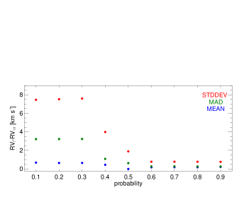
Figure 1: Run of standard deviation (STDDEV, red), median absolute deviation (MAD, green), and mean (blue) of the difference between the mean RV obtained using different probability cuts and those obtained only for stars with p$=$1 for the 30 clusters with 4 or more stars with the highest probability.

In Fig. 1 we have plotted the standard deviation (STDDEV, red), median absolute deviation (MAD; green), and mean (blue) of the difference between the mean RV obtained using different probability cuts, RV_i, and the value obtained using only stars with p=1, RV_1.0. The mean of the difference does not change significantly for the different cuts, but we see a decrease at $p>0.5$. The MAD is almost flat for p$\geq$0.4 and it differs significantly between p=0.3 and p=0.4. The same trend is observed in the standard deviation but in this case the main increase is observed between p=0.4 and p=0.5. As a result of this analysis we limit our analysis to those stars with p$\geq$0.5. We note that Soubiran et al. (2018) considered members with probabilities p$\geq$0.4 based on other reference values from the literature.

In total we found 1406 stars with $p\geq$0.5 belonging to 131 open clusters in common between APOGEE DR14 and Gaia-DR2 (Cantat-Gaudin et al., 2018). These 131 systems are listed in Table 2. A few examples of colour-magnitude diagrams (CMD) of these clusters are shown in Fig. 2. The individual stars are listed in Table LABEL:A1.

Table 2: The 131 open clusters in common between APOGEE DR14 and Cantat-Gaudin et al. (2018).

Cluster	Star	RV	$\sigma_{RV}$	eRV	Nr	RVlit	$\sigma_{RV,lit}$	Nrlit	RVGDR2	$\sigma_{GDR2}$	NrGDR2	[Fe/H]	$\sigma_{[Fe/H]}$	e[Fe/H]	Nr	[Fe/H]lit	$\sigma_{[Fe/H],lit}$	Nrlit	Ref.
	type	(km s-1)				(km s-1)			(km s-1)			(dex)				(dex)
Alessi 20	MS	-14.89		0.37	1	-11.5	0.01	2	-5.04	3.3	7								1
ASCC 124	MS	-23.35	0.54	0.38	2
ASCC 16	MS	17.41		0.62	1				23.18	3.4	15
ASCC 21	MS	16.30	5.66	1.30	19	18.57	2.12	9	18.7	4.45	9	0.01	0.09	0.03	10				2
Basel 11b	RGB	2.68	0.06	0.04	2				3.43	1.46	3	0.014	0.05	0.04	2
Berkeley 17	RGB	-73.34	0.41	0.13	9	-73.4	0.4	7	-71.95	1.77	7	-0.10	0.04	0.01	9	-0.11	0.03	7	3
Berkeley 19	RGB	17.44	0.0	0.08	1				17.65	0.42	1	-0.22		0.01	1
Berkeley 29	RGB	25.27	0.53	0.30	3	24.8	1.13	11	50.58	0.94	1								1
Berkeley 31	RGB	57.87	0.65	0.46	2	61.0	3.75	17				-0.305	0.037	0.026	2	-0.31	0.06	2	1,12
Berkeley 33	RGB	77.80	0.56	0.28	4	76.6	0.5	5	78.82	1.12	4	-0.23	0.11	0.05	4				2
Berkeley 43	RGB	29.712		0.136	1				29.15	1.42	9	0.00		0.01	1
Berkeley 53	RGB	-35.77	0.82	0.29	8	-36.3	0.5	4	-34.9	1.81	7	-0.02	0.03	0.01	6	0.00	0.02	5	3

(1) Kharchenko et al. (2013); (2) Dias et al. (2002); (3) Donor et al. (2018); (4) Casamiquela et al. (2016); (5) Carrera et al. (2017); (6) Donati et al. (2015b); (7) Magrini et al. (2017); (8) Schiappacasse-Ulloa et al. (2018); (9) Blanco-Cuaresma et al. (2015); (10) Heiter et al. (2014); (11) Začs et al. (2011); (12) Friel et al. (2010); (13) Monroe & Pilachowski (2010).

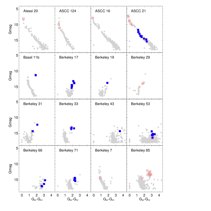
Figure 2: Gaia DR2 colour-magnitude diagrams for OCs with stars in common with APOGEE DR14. Grey circles are Gaia DR2 stars with a membership probability above 0.5. Open red squares are stars in common with APOGEE DR14 used in the RV determination (see text for details). Filled blue squares are objects used in the [Fe/H] analysis.

2.2 GALAH

The GALAH survey (De Silva et al., 2015; Martell et al., 2017) is a Large Observing Program using the High Efficiency and Resolution Multi-Element Spectrograph (HERMES, Barden et al. 2010; Sheinis et al. 2015). HERMES provides simultaneous spectra of up to 392 objects with a resolution power of 28,000 in four wavelength bands: 4713-4903 Å (blue arm), 5648-5873 Å (green arm), 6478-6737 Å (red arm), and 7585-7887 Å (infrared arm). The GALAH second Data Release (DR2 Buder et al., 2018) includes about 340,000 stars. Radial velocities and their uncertainties in GALAH are computed by cross-correlating the observed spectra with 15 synthetic AMBRE spectra (de Laverny et al., 2012). The typical RV uncertainty in GALAH DR2 is $\sim$0.1 km s^-1 (Zwitter et al., 2018). GALAH chemical analysis is performed in two steps (see Buder et al., 2018, for details). Briefly, the stellar parameters and abundances of a training set of about 10,500 stars are first found by spectral synthesis with the Spectroscopy Made Easy code (SME, Valenti & Piskunov, 1996; Piskunov & Valenti, 2017). The obtained results are then used to train the The Cannon (Ness et al., 2015) data-driven algorithm to find stellar parameters and abundances for the whole GALAH sample.

According to Buder et al. (2018), open clusters are not part of the fields already released by GALAH but are observed by several separate programmes with HERMES, i.e. with the same instrument. Some OCs were used in Buder et al. (2018) as a test of the GALAH results (see later for further details). Kos et al. (2018a) combined Gaia DR2 and GALAH to study five candidate low-density, high-latitude clusters, finding that only one of them, NGC 1901, can be considered a cluster, while the others are only chance projections of stars. Similar results have been found by Cantat-Gaudin et al. (2018) for many high-latitude candidate clusters.

While GALAH and the linked private projects are targeting OCs on purpose, there may be also cluster stars observed serendipitously and we looked for them. After cross-matching the Cantat-Gaudin et al. (2018) high-probability members ($p\geq 0.5$) with GALAH DR2 we found 122 stars in 14 OCs. We list in Table LABEL:A2 parameters from Gaia ($G$, $G_{BP}$-$G_{RP}$, $\varpi$, $\mu_{\alpha*}$, $\mu_{\delta}$) and GALAH (RV, T_eff, $\log g$, $v\sin i$, [Fe/H]) for the individual stars. Among them, we selected those stars without problems during The Cannon analysis, labelled as flag_cannon=0, or that need only some extrapolation, flag_cannon=1 (see Buder et al., 2018, for more details). After applying these constrains we are left with 82 stars in 14 clusters.

Since the majority of the clusters are young, the stars targeted are mostly on the main-sequence (MS; there are giants only in NGC 2243 and NGC 2548). Furthermore, they are often of early spectral types and may show high rotational velocities. Their RV determination is then less reliable (the same is valid for metallicity, see Sect. 4.2) and we tried to keep only the stars with $v\sin i$ values lower than 20 km s^-1. In addition, candidate members according to astrometry show discrepant RVs in some clusters (see Table LABEL:A2). To select only the highest probability cluster members based both on astrometry and RV, we used the average cluster RVs determined by Soubiran et al. (2018) using Gaia DR2 data (at least 4 stars were sampled in all these OCs). This affects only five clusters: ASCC 21, Alessi 24, Alessi-Teutsch 12, NGC 5640, and Turner 5. One discrepant radial velocity star have been discarded in each of them.

After all this weeding we ended up with 29 stars in 14 clusters; in half of the cases only one star survived the selections. The properties of these stars are summarised in Table 6, Fig. 3 shows the CMD of the 14 OCs and the stars used in our analysis indicated, while Table 3 lists the 14 OCs and their mean RV and metallicity.

Figure 3: As in Fig. 2 for the 14 clusters in the GALAH sample. Note that one star in NGC 2516 and one in Turner 5 have no colour information and were arbitrarily plotted at $G_{BP}$-$G_{RP}$=0.

Table 3: Properties of the 14 open clusters in common between GALAH DR2 and Cantat-Gaudin et al. (2018).

Cluster	Star	RV	$\sigma_{RV}$	eRV	$\left\langle{\rm v}\sin i\right\rangle$star	Nr	RVGDR2	$\sigma_{GDR2}$	NrGDR2	[Fe/H]	$\sigma_{[Fe/H]}$	e[Fe/H]	Nr	[Fe/H]lit	$\sigma_{[Fe/H],lit}$	Nrlit	Ref.
	type	(km s-1)					(km s-1)			(dex)				(dex)
Alessi 24	MS	10.44		0.11	11.63	1	12.32	2.24	14	-0.13		0.07	1
Alessi 9	MS	-5.64		0.11	5.70	1	-6.44	1.14	39	-0.06		0.07	1
Alessi-Teutsch 12	MS	-11.00		0.12	5.35	1	-5.88	3.54	6	0.40		0.08	1
ASCC 16	MS	22.01		0.17	38.82	1	23.18	3.40	15	-0.08		0.06	1
ASCC 21	MS	20.05		1.06	19.99	1	18.70	4.45	9	-0.13		0.08	1
Collinder 135	MS	17.08	0.96	0.68	18.31	2	16.03	2.21	51	-0.09	0.03	0.02	2
Collinder 359	MS	8.30		1.79	57.53	1	5.28	3.25	12	-0.66		0.08	1
Mamajek 4	MS	-28.09	2.19	0.98	6.95	5	-26.32	3.17	34	0.09	0.17	0.08	5
NGC 2243	RGB	59.32	0.57	0.23	7.36	6	59.63	1.06	4	-0.31	0.05	0.02	6	-0.43	0.04	16	1
NGC 2516	MS	26.01	1.40	0.81	34.10	3	23.85	2.01	132	-0.26	0.05	0.03	3	0.06	0.05	13	1
NGC 2548	RGB	8.45	0.40	0.28	5.20	2	8.85	1.08	14	0.16	0.01	0.04	2
NGC 3680	MS	2.98		1.99	33.54	1	1.74	1.36	30	-0.26		0.07	1	-0.01	0.06	10	2
NGC 5460	MS	-5.16	0.31	0.22	23.79	2	-4.61	2.77	5	-0.32	0.15	0.11	2
Turner 5	MS	-2.83	0.09	0.07	11.77	2	-3.49	1.93	6	0.02	0.17	0.12	2

(1) Magrini et al. (2017); (2) Netopil et al. (2016)

3 Radial Velocities

3.1 APOGEE

The mean RV for each cluster has been computed using equation 1 described above. The internal velocity dispersion is derived as

$$\sigma_{RV}=\sqrt{\frac{n}{n-1}\times\frac{\sum_{i}g_{i}\times(RV_{i}-RV)^{2}}{\sum_{i}g_{i}}}$$ (2)

with an uncertainty of

$$e_{RV}=\frac{\sigma_{RV}}{\sqrt{n}}$$ (3)

For those clusters with only one star sampled we did not compute $\sigma_{RV}$ and we assumed $e_{RV}=RV\_scatter_{i}$. The obtained values are listed in Table 2. In total we have determined mean RV for 131 clusters. For 78 of them, about 65% of the total, this RV determination is based on less than 4 stars and the values have to be taken with caution. For the other 53 systems the RV is determined from 4 stars or more. In principle these values are more reliable except if they show a large $\sigma_{RV}$. Large $\sigma_{RV}$ values can be due to undetected binaries but also by residual field stars contamination.

For the majority of the OCs the RV determination is based on either giant or MS stars. In general, the systems whose RVs have been determined from MS stars have larger $\sigma_{RV}$ values because of the larger RV uncertainties for these stars. There are 9 clusters with both kind of stars sampled: Berkeley 71, Berkeley 85, Berkeley 9, King 7, NGC 1664, NGC 1857, NGC 2682, NGC 6811, and NGC 7782. Except for NGC 1664, at least 5 stars have been observed in each of them. There are not significant differences in the mean RV values if we use only MS stars or giants.

There are 104 clusters in common with the recent work by Soubiran et al. (2018). They derived mean RVs for 861 OCs based on the Gaia DR2 catalogue and the RVs obtained with the Gaia RVS instrument, using a pre-selection done on our same astrometric membership probabilities (Cantat-Gaudin et al., 2018). The top panel of Fig. 4 shows the comparison between the RV for the 104 clusters in common. The RV differences, $\Delta RV$, defined as $RV_{\textit{Gaia}\leavevmode\nobreak\ DR2}-RV_{APOGEE}$, are shown in the bottom panel of Fig. 4. In general, there is a very good agreement between both samples for most of the clusters in spite of the Gaia DR2 typical uncertainties being larger than 2.5 km s^-1. The median difference between Gaia DR2 and our APOGEE sample is 0.4 km s^-1 with a median absolute deviation of 3.2 km s^-1. However, there are a few cases that show significantly different RVs. All these clusters have only a few sampled stars either in our APOGEE sample or in the Gaia DR2 sample. For example, in the case of the system with the largest difference, IC 4996, the values in both samples have been obtained for only one candidate member. The RV from the star observed by APOGEE is 78.5$\pm$0.3 km s^-1, while in Gaia DR2, from a different star, the obtained value is -29.1$\pm$2.9 km s^-1. None of them is similar to the value of -2.5$\pm$5.7 km s^-1 based on 4 stars cited in Kharchenko et al. (2013), or to the value of $-12\pm 5$ km s^-1 found from pre-main-sequence stars by Delgado et al. (1999). More data are required in cases such as this.

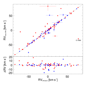
Figure 4: Comparison between RV derived from APOGEE DR14 and Gaia DR2. Blue points are clusters with 4 or more stars while red points are systems with less then 4 stars.

In addition to the Soubiran et al. (2018) work, we have compiled other RV determinations in the literature using the updated version of the DAML and MWSC catalogues as starting point and adding recent determinations available in the literature. In total we have compiled RVs for 75 of the 131 OCs in our sample (see Table 2 where also references are indicated). The comparison between the RV values obtained in this work and the literature is shown in the top panel of Fig. 5, while the bottom panel shows the behaviour of the differences between them. As before, the largest discrepancies are generally observed for those clusters with less than 4 stars sampled (red points). In fact, the literature determinations for these clusters are also based on 4 objects or less, with the exception of NGC 457. In Czernik 20 and Trumpler 2 we have 7 and 5 stars, respectively. For Trumpler 2 we found a large $\sigma_{RV}$ which implies that our RV determination is not very reliable (see below). In the case of Czernik 20 the literature value has been obtained from a single star with an uncertainty of 10 km s^-1. This value is much larger than the internal dispersion found in our work from 7 stars. For this reason we consider our RV determination more reliable.

To our knowledge this is the first RV determination for 16 clusters: ASCC 124, Berkeley 7, Berkeley 98, Czernik 18, Dolidze 3, FSR 0826, FSR 0941, Kronberger 57, L 1641S, NGC 1579, NGC 6469, Ruprecht 148, Stock 4, Teutsch 1, Teutsch 12, and Tombaugh 4. In the case of L 1641S our RV determination is based on 43 stars with an internal dispersion $\sigma_{RV}\sim$2 km s^-1. Two clusters, Berkeley 98 and Teutsch 12, have 5 potential members with a $\sigma_{RV}$ of 3.3 and 2.3 km s^-1, respectively. Due to the number of objects used in these three systems to derive their mean RV and given their small $\sigma_{RV}$, we believe that our determinations are reliable. For the remaining clusters the RV determinations are based on one star only, with the exception of ASCC 124 and Czernik 18 with two and three stars, respectively. As commented before, their RV are less reliable.

Eight systems have $\sigma_{RV}$ values larger than 6 km s^-1. The largest internal dispersion is obtained for NGC 366 with $\sigma_{RV}\sim$21 km s^-1. This value has been obtained from 4 stars with $p\geq$0.9 but with very different individual RV. In the case of NGC 2183 we found $\sigma_{RV}\sim$13 km s^-1. This value is obtained from 5 stars with RVs between 7.4 and 43.1  km s^-1. However the two stars with the highest priorities, $p$=1 and 0.8, have RV of 28.9$\pm$0.2 and 25.4$\pm$0.1 km s^-1, respectively. All the stars in NGC 2183 have only one APOGEE visit and therefore the RV determinations are more uncertain. The remaining six clusters (Koposov 36, NGC 2304, NGC 7086, Rosland 6, Trumpler 2, and Trumpler 3) have $\sigma_{RV}$ between 6 and 10 km s^-1. The number of potential members sampled by APOGEE in these systems is between 4 and 8 stars. Almost all the stars in these clusters have higher membership probabilities, $p\geq$0.8. Since all of them are main-sequence stars, their individual RV determination can be affected by the large rotational velocities. Three of these clusters have determination of their RV in the literature (see Table 2). In spite of the large RV dispersion observed in two of these clusters, NGC 2304 and NGC 7086, we find a good agreement with the values listed in the literature (Wu et al., 2009; Kharchenko et al., 2013).

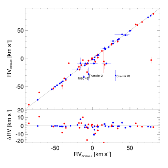
Figure 5: Comparison between RV derived from APOGEE DR14 and literature. Blue and red points have the same meaning as in Fig 4.

3.2 GALAH

Figure 6: Comparison between RV derived from GALAH DR2 and Gaia DR2, colour-coded according to $\left\langle{\rm v}\sin i\right\rangle$.

The same procedure followed above for APOGEE has been used to derive the mean RV, internal velocity dispersion, and uncertainty for the 14 OCs in the GALAH sample. The obtained values are listed in Table 3.

Radial velocities for all the clusters in the GALAH sample have been determined previously by Soubiran et al. (2018) from Gaia DR2. The comparison between the RVs measured by GALAH and those by Gaia DR2 for the 14 clusters is shown in Fig. 6. The median difference between Gaia DR2 and GALAH is 0.3 km s^-1 with a median absolute deviation of 1.5 km s^-1. The RVs are in reasonable agreement taken into account that the individual RV uncertainties in the Gaia DR2 are on average of 2.5 km s^-1. The largest differences for some clusters (e.g. Collinder 359 and NGC 2517) are explained by their large average $\left\langle{\rm v}\sin i\right\rangle$ values.

The clusters NGC 2243 and NGC 2516 have been observed also by Gaia-ESO and their mean RV are +60.2 (rms 1.0) km s^-1 and +23.6 (rms 0.8) km s^-1, respectively (Jackson et al., 2016; Magrini et al., 2017). For NGC 2243 we obtained 59.3 km s^-1 with $\sigma_{RV}$=0.6 km s^-1 from 6 giant stars. The values are in good agreement within the uncertainties. In the case of NGC 2516 we obtained 26.0 km s^-1 with $\sigma_{RV}$=1.4 km s^-1 from 3 MS stars. The difference between GALAH and Gaia-ESO mean RV could be due to the fact that the three stars in the GALAH sample have v$\sin i$ larger than 29 km s^-1.

Four of the GALAH clusters are also among the APOGEE systems discussed in previous section. These clusters are ASCC 16, ASCC 21, Collinder 359, and NGC 2243. In the case of NGC 2243 there is a good agreement between the values obtained from both samples in spite of the APOGEE value being based on only one star. For the other three clusters the differences between GALAH and APOGEE are of the order of $\pm$4 km s^-1. This is not a large difference taken into account that all the stars sampled in these clusters by GALAH have $v\sin i$ larger than 20 km s^-1.

4 Metallicity

4.1 APOGEE

Before deriving average metallicity we excluded the stars for which the ASPCAP pipeline is not able to find a proper solution (or not a solution at all) because they are outside of or close to the edges of the synthetic library used in the analysis, e.g. hot stars (see García Pérez et al., 2016; Holtzman et al., 2018, for details). In this case the stars are flagged in ASPCAPFLAG as STAR_BAD or NO_ASPCAP_RESULT, respectively. After rejecting these objecys, the sample is reduced to 862 stars belonging to 90 clusters. Most of the rejected stars are fast rotating or low gravity objects.

Together with the individual iron abundance [Fe/H] for each star, APOGEE DR14 provides the scaled-solar general metallicity, [M/H]. The former is obtained from individual Fe lines whereas the latter is determined as a fundamental atmospheric parameter at the same time as effective temperature, surface gravity, and microturbulent velocity. In this paper we focus on the individual iron abundances. In contrast with the RV case, the average [Fe/H] of each cluster has been obtained as the un-weighted mean of the individual iron abundances. We have computed also $\sigma_{[Fe/H]}$ as the un-weighted standard deviation and $e_{[Fe/H]}$ as $\frac{\sigma_{[Fe/H]}}{\sqrt{n}}$. Again for those clusters with only one sampled star we did not compute the standard deviation, $\sigma_{[Fe/H]}$, and we assume the uncertainty $e_{[Fe/H]}$, as the uncertainty for this star, $\sigma_{[Fe/H],i}$.

The obtained values are listed in Table 2. For 32 systems our [Fe/H] determination is based on 4 stars or more. Except for Berkeley 33, the $\sigma_{[Fe/H]}$ is lower than 0.1 dex, the typical uncertainty in the APOGEE [Fe/H] determination. The [Fe/H] determination for the other 58 clusters is based on less than 4 stars and typically on only one object.

To our knowledge there are previous determinations of iron abundances from high resolution spectra for a third of the total sample. The comparison between the values derived here and the literature (see Table 2 for references) is shown in Fig. 7. In general, there is a very good agreement, with a median difference 0.00 dex with a median absolute deviation of 0.02 dex. This is not unexpected since several OCs have been used as reference to calibrate the whole APOGEE sample assuming values available in the literature (see Holtzman et al., 2018, for details).

For the 57 clusters not studied previously only in 9 of them the metallicity determination is based on 4 or more stars. Two or three stars have been sampled for 16 of these systems. Finally, the metallicity determination for 32 previously unstudied clusters is based on a single star.

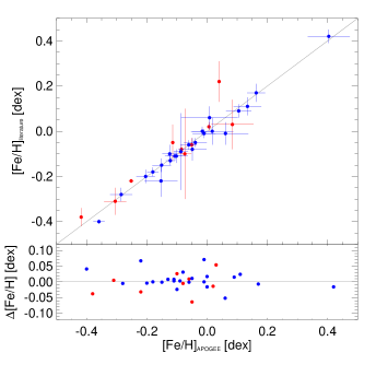
Figure 7: Comparison between [Fe/H] derived from APOGEE DR14 and literature. Red and blue points are clusters with less and more than 4 stars, respectively.

4.2 GALAH

In the case of GALAH the constraints applied initially also ensure that the iron abundance has been determined for all the stars in the sample. The average metallicities for the clusters in the GALAH sample has been derived using the same procedure as in the case of APOGEE. The obtained values are listed in Table 3.

Only in two clusters (Mamajek 4 and NGC 2243) our analysis is based on more than 4 stars. The value obtained here for NGC 2243 is in good agreement with the result obtained by e.g. Magrini et al. (2017) and other literature sources. This cluster is also among the clusters studied in the previous section from APOGEE. Although the APOGEE analysis is based on a single star, the values are in agreement within the uncertainties.

Due to the early spectral type and high rotational velocity of the members, we judged as unreliable the metallicity determination for 6 clusters (ASCC 16, ASCC 21, Collinder 359, NGC 2516, NGC 3680, and NGC 5460). Moreover, their [Fe/H] values have been determined from 3 stars or less. One of these clusters, ASCC 21, has been also analysed from APOGEE data. The values obtained from APOGEE and GALAH samples show a difference of only 0.1 dex, in spite of the large $v\sin i$ and high temperature of the only star in GALAH DR2 for this cluster. Other two of these clusters, NGC 2516 and NGC 3680, have been studied previously in the literature Magrini et al. (e.g. 2017) and Netopil et al. (2016). In comparison with these works, the [Fe/H] values obtained here are about 0.25 dex lower. Buder et al. (2018) discussed possible shortcomings of GALAH DR2 catalogue. They note that the double-step analysis is tailored on single, non-peculiar stars of F, G, and K spectral types and that some systematic trends may be present. In particular, they note difficulties for hot stars (i.e., hotter than late-F spectral type) because they have weaker metal lines, often rotate significantly, and are not present in the training set; all stars hotter than 7000 K are then in extrapolation. Furthermore, there is a trend in the derived temperatures, with hotter stars showing lower temperatures than the comparison samples (e.g. the Gaia Benchmark stars or stars for which the IRFM was available, their Fig. 14). In turn, this implies a trend towards lower metallicities. This is noticeable, for instance, in the T_eff, $\log g$ diagrams for open clusters (their Fig. 19), with brighter MS stars showing systematically lower abundances. This is also what we found for NGC 2516 and NGC 3680.

In summary, the GALAH DR2 sample provides the first [Fe/H] determination for 10 clusters although with different degrees of reliability because of the large rotational velocities of some of the stars analysed.

5 Other elements

5.1 APOGEE

Although APOGEE DR14 provides abundances for 22 chemical elements, not all of them are completely reliable (see Jönsson et al., 2018; Holtzman et al., 2018). For this reason we limit our analysis to the elements that show small systematic differences in comparison with other literature samples according to Jönsson et al. (2018). This includes $\alpha$-elements (Mg, Si, and Ca) and proton-capture elements (Na and Al) as well as elements of the iron-peak group (Cr, Mn and Ni). For each element we have excluded the stars flagged by ASPCAP with problems in the abundance determination.

We have been able to determine abundances for all the 90 clusters with iron abundances for the majority of elements: Mg, Si, Ca, Mn, and Ni (Table LABEL:tab:apogee_abun). Aluminum abundances have been derived for 89 systems (the missing cluster, IC 1805, has only one star). Several stars have been rejected in the determination of chromium content so that the abundances of this element have been determined for 84 systems. Sodium is the element for which we reject more stars, with Na abundances obtained for only 65 of the 90 clusters. The abundance of Na is determined in APOGEE from two weak and probably blended lines, that are easily measured only in GK giants (see Jönsson et al., 2018, for details). Therefore, Na abundances cannot be determined for many stars in the sample because they are outside this range.

As before, the values obtained here should be used with caution. Only the abundances obtained for at least 4 stars and with small internal dispersion can be considered reliable. Owing to the large heterogeneity of the abundance determinations available in the literature we have not tried a comparison.

In Fig. 8 we show trends of the abundance ratios obtained with [Fe/H] and among all other elements. The most discrepant values are due to clusters with less than 4 stars sampled (grey points). Clusters with more than 4 stars analysed show, in general, a scatter compatible with the typical uncertainties. The exceptions are Na and in less degree Cr. The well know differences of Na abundances between dwarfs and giants due to extra-mixing can explain this scatter. There is one cluster, NGC 2168, for which we obtained [Ca/Fe]=-0.17 dex from 10 stars. Although this value is lower than the bulk, its dispersion of $\sigma_{[Ca/Fe]}$=0.21 dex (probably due to the difficulties in measuring main-sequence stars in APOGEE) makes it still compatible with the majority.

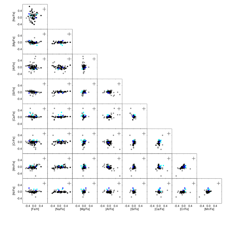
Figure 8: Plot of the abundance ratios for APOGEE and GALAH clusters. Grey and black circles are APOGEE clusters with less and more than 4 stars in the determination of [Fe/H], respectively. Cyan and blue circles are GALAH clusters with less and more than 4 stars in the determination of [Fe/H], respectively. Typical error bars have been plotted in top-right corners.

5.2 GALAH

The GALAH DR2 provides abundances for 23 chemical elements including iron (see Buder et al., 2018). For homogeneity with the APOGEE sample, we computed average abundances for the same 8 elements than above. Following the Buder et al. (2018) recommendations we only use those stars that do not have problems in the determination of the abundance of a given element (i.e. flag_X_FE=0). Moreover, we also excluded those clusters with $v\sin i>$20 km s^-1 because the values obtained for these stars are not reliable. As a result of this, abundances have been determined for only 7 clusters and not for all elements. The obtained values are listed in Table LABEL:A3.

The GALAH ratios have been plotted in Fig. 8 as cyan (less than 4 stars) and blue (more than 4 objects) filled circles. Although the GALAH sample is small, we see that there are no significant differences between APOGEE and GALAH samples for any of the elements studied. Only the metal-poor cluster NGC 2243 seems to have a large [Ni/Fe] ratio, +0.22 dex ($\sigma_{[Ni/Fe]}$=0.14 dex) obtained from 5 stars, in comparison with other APOGEE clusters of the same [Fe/H]. This cluster is the only one in common with the APOGEE sample with reliable abundances in GALAH. For direct comparison, in the case of APOGEE we obtained [Ni/Fe]=0.01 dex from a single star with e_[Ni/Fe]=0.02 dex. Also for Si we found a difference larger than the the uncertainties: [Si/Fe]=0.09 and -0.04 dex from APOGEE and GALAH, respectively. Again the APOGEE value has been derived from a single star with e_[Si/Fe]=0.03 dex while the GALAH one has been determined from 4 stars with $\sigma_{[Ni/Fe]}$=0.04 dex. For the other elements studied the ratios obtained from APOGEE and GALAH samples are in agreement within the uncertainties.

6 Galactic trends

As commented in Sect. 1, information about the chemical composition of OCs is necessary to address a variety of astrophysical topics. A clear example of the applicability of the sample obtained in this work is the study of the chemical gradients in the Galactic disk. Generally the chemical gradients in the Galactic disk are studied using iron (e.g. Netopil et al., 2016), which is produced in approximately equal measure by core collapse and type Ia supernovae. Additionally, we present here the behaviour of magnesium as best representative of the $\alpha$-elements. Not only the production of magnesium is dominated by core collapse supernovae, but also the Mg abundances derived by APOGEE and GALAH show the best agreement with external measurements in comparison with other elements of this group (Jönsson et al., 2018; Buder et al., 2018). Given the much larger number of clusters involved, the APOGEE data dominate the following discussion. The run of [Fe/H] as a function of Galactocentric distance, R_gc, is plotted in the bottom panel of Fig. 9, while the top panel shows the behaviour of [Mg/Fe] with R_gc. Galactocentric distances have been computed by Cantat-Gaudin et al. (2018) from Gaia-DR2 parallaxes; we refer the reader to that paper for details about the distance determination.

The clusters with 4 or more stars, with more trustful measurements (blue symbols), cover a range in R_gc between $\sim$6.5 and $\sim$13 kpc. Grey symbols are clusters with less reliable measurements. There is no full agreement about the slope of the gradient in this R_gc range and we can found in the literature values between $\frac{d[FeH]}{dR_{gc}}\sim$-0.035 dex kpc^-1 (Cunha et al., 2016) and -0.1 dex kpc^-1 (Jacobson et al., 2016). Using all the clusters in the APOGEE and GALAH samples with at least 4 stars we found $\frac{d[Fe/H]}{dR_{gc}}$=-0.052$\pm$0.003 dex kpc^-1 (red dashed line). The slope of the gradients may depend on the presence of the innermost cluster in the sample, NGC 6705, and the most metal-rich one, NGC 6791. Both are peculiar clusters. NGC 6705 is a young metal-rich system (see e.g. Cantat-Gaudin et al., 2014) with an unexpected high $\alpha$-elements abundance (Casamiquela et al., 2018; Magrini et al., 2017). On the contrary, NGC 6791 is an intriguing old very metal-rich and massive system located almost 1 kpc above the Galactic plane. It has been suggested that NGC 6791 has likely migrated to its current location from its birth position (Linden et al., 2017) or even has an extragalactic origin (Carraro et al., 2006) although both claims are disputed. If we exclude these two clusters from the analysis, the [Fe/H] gradient flattens to -0.047$\pm$0.004 dex kpc^-1. This does not imply that former value is preferred. It only shows how the gradient changes as a function of the outliers.

If we separate the clusters in two groups inside and outside R${}_{gc}=$11 kpc we find $\frac{d[Fe/H]}{dR_{gc}}$=-0.077$\pm$0.007 dex kpc^-1 in the inner region and $\frac{d[Fe/H]}{dR_{gc}}$=0.018$\pm$0.009 dex kpc^-1 for the outer region. A similar result has been reported previously (e.g. Carrera & Pancino, 2011; Andreuzzi et al., 2011; Frinchaboy et al., 2013; Cantat-Gaudin et al., 2016, among many). If we exclude the two metal-poor cluster at R${}_{gc}\sim$11 kpc (NGC 2243 and Trumpler 5) the slope increases until $\frac{d[Fe/H]}{dR_{gc}}$=-0.04$\pm$0.01 dex kpc^-1. Therefore, the behaviour in the outermost region is highly dependent on these clusters. All these results are in good agreement with Donor et al. (2018) who also used chemical abundances obtained from APOGEE DR14 with a different cluster membership selection. Furthermore, the observed gradient may change as a function of the age of the clusters used in the analysis (e.g. Friel et al., 2002; Andreuzzi et al., 2011; Carrera & Pancino, 2011; Jacobson et al., 2016). However, age is yet unknown for a large fraction of our clusters and we postpone to a forthcoming paper a detailed analysis of the evolution of the gradient with the age of the clusters.

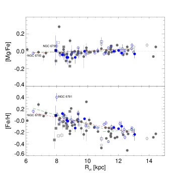
Figure 9: Gradient in [Mg/Fe] (top) and [Fe/H] (bottom) as a function of R_gc for APOGEE (circles) and GALAH (triangles) clusters. Grey symbols are clusters with less than four stars. Blue symbols are clusters with 4 or more stars sampled. Filled symbols are the clusters for which this is the first metallicity determination from high resolution spectroscopy. Green and orange lines show different linear fits (see text for details). The positions of NGC 6705 and NGC 6791 have been marked.

The run of $\alpha$-element abundances as a function of Galactocentric radius is still an open discussion (e.g. Donati et al., 2015a; Cantat-Gaudin et al., 2016). Donor et al. (2018) reported a mild positive gradient for magnesium and other $\alpha$-elements such as oxygen or silicon. On contrast, Yong et al. (2012) and Friel et al. (2014) did not found any dependence with R_gc. A similar result has been found by Cantat-Gaudin et al. (2016) and also by Magrini et al. (2017) using OCs and field stars homogeneously analysed by the $Gaia$-ESO survey. The top panel of Fig. 9 does not show a clear trend. The slope of the linear fit (red dashed line) to the whole range of R_gc is $\frac{d[Mg/Fe]}{dR_{gc}}$=0.003$\pm$0.002 dex kpc^-1. The clusters within R${}_{gc}\sim$10 kpc have, in general, a [Mg/Fe] below the solar one. This includes the innermost cluster, NGC 6705, for which Casamiquela et al. (2018) has reported a higher value of [Mg/Fe]=+0.14$\pm$0.07 dex, in agreement with the $Gaia$-ESO result of $+0.10\pm 0.07$ (Magrini et al., 2017). There is a group of clusters at $\sim$8 kpc which [Mg/Fe] are compatible with the solar one within the uncertainties. At R${}_{gc}\sim$8.5 kpc the [Mg/Fe] is clearly lower than the solar. From there the [Mg/Fe] ratio increases until $\sim$10 kpc and it flattens from thereof. This behaviour has been reported previously in the literature (e.g. Cantat-Gaudin et al., 2016; Magrini et al., 2017) and it has been predicted by Galactic chemical evolution models (e.g. Minchev et al., 2014; Kubryk et al., 2015b, a; Grisoni et al., 2018).

The existence of a vertical gradient is also controversial. Several authors do not find any trend of [Fe/H] with the distance to the Galactic plane, Z (e.g. Jacobson et al., 2011; Carrera & Pancino, 2011). Instead, other studies reported the existence of a vertical gradient with a slope between -0.34 and -0.25 dex kpc^-1 (e.g Piatti et al., 1995; Carraro et al., 1998). In Fig.10 we plot [Fe/H] and [Mg/Fe] as a function of Z (bottom and upper panel, respectively). In both cases there are no hints of the existence of vertical gradients in agreement with most previous studies. We also confirm that clusters located at larger Galactocentric distances cover a larger range of Z. The exception is NGC 6791 located at R${}_{gc}\sim$8 kpc and with a height above the plane of $Z\sim$900 pc. We have already commented that this is a peculiar and not well understood system.

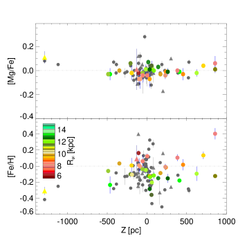
Figure 10: The run of [Mg/Fe] (top) and [Fe/H] (bottom) as a function of the distance to the Galactic plane $Z$. Symbols are as in Fig. 9.

7 Summary

Using Gaia DR2 Cantat-Gaudin et al. (2018) determined astrometric membership probabilities for stars belonging to 1229 open clusters. We have cross-matched this catalogue with the latest data releases of two of the largest Galactic high-resolution spectroscopic surveys, APOGEE and GALAH, with the goal of finding high probability OC members.

• In the case of APOGEE we have detected stars belonging to 131 clusters for which we have determined average radial velocities. For 46 systems our determination is based on 4 or more stars. To our knowledge this is the first radial velocity determination for 16 systems. For the other clusters there is a good agreement between the obtained values and those available in the literature. [Fe/H] has been obtained for 90 open clusters, almost two thirds of them without previous determinations in the literature. Finally, for the same 90 clusters we have also determined abundances for six elements: Na, Mg, Al, Si, Ca, Cr, Mn, and Ni.

• In the case of GALAH we have found stars belonging to 14 clusters for which we have determined both radial velocities and iron abundances. Except for two clusters, NGC 2243 and NGC 2548, the GALAH sample is composed by main-sequence stars, in some cases with significant $v\sin i$ values. These 14 clusters have previous radial velocity determination from Gaia DR2. Excluding the two clusters in common with APOGEE sample, nine of these systems do not have previous determinations in the literature from high resolution spectroscopy. For seven clusters we have determined abundances for the same chemical elements that in the case of APOGEE.

In summary, to our knowledge this is the first RV determination from high resolution spectra for 16 open clusters. In the same way, we provide for the first time iron abundances for 39 open clusters, 30 from APOGEE and 9 from GALAH, respectively.

The obtained catalogue of chemical abundances has been used to investigate the existence of radial and vertical trends using the distances computed from Gaia DR2. Our findings are in agreement with previous investigations where the radial [Fe/H] gradient appears to flatten in the outer region. We do not find any hint, at least above the 1$\sigma$ level, of the existence of a vertical metallicity gradient.

Appendix A Tables

Table 4: Information on APOGEE DR14 stars in common with candidate members in Gaia DR2 (Cantat-Gaudin et al. 2018).

Cluster	star_id	source_id	RA	DEC	$\varpi$	$\sigma_{\varpi}$	$\mu_{\alpha*}$	$\sigma_{\mu_{\alpha*}}$	$\mu_{\delta}$	$\sigma_{\mu_{\delta}}$	$G$	$G_{BP}-G_{RP}$	p	RV	$\sigma_{RV}$	Teff	$\sigma_{\rm Teff}$	$\log g$	$\sigma_{\log g}$	[Fe/H]	$\sigma_{[Fe/H]}$
ASCC 124	2M22450300+4613588	1982689777242358912	341.26249155537	46.23300470968	1.3276718736945818	0.04611155225642544	0.2996917390783982	0.06885027846654153	-2.0589048051205565	0.0662293265210654	9.92051	0.12712765		0.5	-18.1821	0.673

Table 5: Information on GALAH DR2 stars in common with candidate members in Gaia DR2 (Cantat-Gaudin et al. 2018).

CLUSTER	star_id	source_id	RA	DEC	$\varpi$	$\sigma_{\varpi}$	$\mu_{\alpha*}$	$\sigma_{\mu_{\alpha*}}$	$\mu_{\delta}$	$\sigma_{\mu_{\delta}}$	$G$	$G_{BP}-G_{RP}$	p	RV	$\sigma_{RV}$	f_c	Teff	$\sigma_{\rm Teff}$	$\log g$	$\sigma_{\log g}$	[Fe/H]	$\sigma_{[Fe/H]}$	$v\sin i$	$\sigma_{v\sin i}$
ASCC 16	05251613+0231412	3234352820498417024	81.3172531	2.5281074	2.809	0.058	1.187	0.09	-0.546	0.075	10.041	0.231	0.6	19.85	0.18	1	7557	48	4.45	0.14	-0.25	0.06	23.92	0.83

Table 6: Individual stars in the GALAH DR2 clusters retained in the analysis.

Cluster	star_id	source_id	$G$	$G_{BP}-G_{RP}$	RV	Teff	$\log g$	[Fe/H]	$v\sin i$	flagcannon
ASCC 16	05242648+0126492	3222160885813451776	11.044314	0.81302357	22.0104529617	5870.960626083559	4.205298815473945	-0.07787835749222094	33.6240327478691	1

Table 7: Abundances obtained for OCs in the APOGEE sample.

Cluster	Na	$\sigma_{Na}$	$e_{Na}$	NrNa	Mg	$\sigma_{Mg}$	$e_{Mg}$	NrMg	Al	$\sigma_{Al}$	$e_{Al}$	NrAl	Si]	$\sigma_{Si}$	eSi	NrSi	Ca	$\sigma_{Ca}$	eCa	NrCa	Cr	$\sigma_{Cr}$	eCr	NrCr	Mn	$\sigma_{Mn}$	eMn	NrMn	Ni	$\sigma_{Ni}$	eN	NrNi
ASCC 21					-0.07	0.04	0.01	10	0.04	0.12	0.04	10	-0.02	0.06	0.02	10	0.04	0.07	0.03	8	-0.21	0.12	0.08	2	-0.09	0.04	0.01	10	-0.07	0.05	0.02	10

Table 8: Mean [X/Fe] abundance ratios for the GALAH clusters.

Cluster	Na	$\sigma_{Na}$	$e_{Na}$	NrNa	Mg	$\sigma_{Mg}$	$e_{Mg}$	NrMg	Al	$\sigma_{Al}$	$e_{Al}$	NrAl	Si]	$\sigma_{Si}$	eSi	NrSi	Ca	$\sigma_{Ca}$	eCa	NrCa	Cr	$\sigma_{Cr}$	eCr	NrCr	Mn	$\sigma_{Mn}$	eMn	NrMn	Ni	$\sigma_{Ni}$	eN	NrNi
Alessi 24	0.11	0.0	0.05	1	-0.11	0.0	0.07	1	-0.1	0.0	0.04	1	0.07	0.0	0.07	1	0.12	0.0	0.05	1	-0.01	0.0	0.05	1	-0.03	0.0	0.06	1	0.01	0.0	0.06	1

Table 9: The 131 open clusters in common between APOGEE DR14 and Cantat-Gaudin et al. (2018).

Cluster	Star	RV	$\sigma_{RV}$	eRV	Nr	RVlit	$\sigma_{RV,lit}$	Nrlit	RVGDR2	$\sigma_{GDR2}$	NrGDR2	[Fe/H]	$\sigma_{[Fe/H]}$	e[Fe/H]	Nr	[Fe/H]lit	$\sigma_{[Fe/H],lit}$	Nrlit	Ref.
	type	(km s-1)				(km s-1)			(km s-1)			(dex)				(dex)
Alessi 20	MS	-14.89		0.37	1	-11.5	0.01	2	-5.04	3.3	7								1
ASCC 124	MS	-23.35	0.54	0.38	2
ASCC 16	MS	17.41		0.62	1				23.18	3.4	15
ASCC 21	MS	16.30	5.66	1.30	19	18.57	2.12	9	18.7	4.45	9	0.01	0.09	0.03	10				2
Basel 11b	RGB	2.68	0.06	0.04	2				3.43	1.46	3	0.014	0.05	0.04	2
Berkeley 17	RGB	-73.34	0.41	0.13	9	-73.4	0.4	7	-71.95	1.77	7	-0.10	0.04	0.01	9	-0.11	0.03	7	3
Berkeley 19	RGB	17.44	0.0	0.08	1				17.65	0.42	1	-0.22		0.01	1
Berkeley 29	RGB	25.27	0.53	0.30	3	24.8	1.13	11	50.58	0.94	1								1
Berkeley 31	RGB	57.87	0.65	0.46	2	61.0	3.75	17				-0.305	0.037	0.026	2	-0.31	0.06	2	1,12
Berkeley 33	RGB	77.80	0.56	0.28	4	76.6	0.5	5	78.82	1.12	4	-0.23	0.11	0.05	4				2
Berkeley 43	RGB	29.712		0.136	1				29.15	1.42	9	0.00		0.01	1
Berkeley 53	RGB	-35.77	0.82	0.29	8	-36.3	0.5	4	-34.9	1.81	7	-0.02	0.03	0.01	6	0.00	0.02	5	3
Berkeley 66	RGB	-50.14	0.21	0.09	5	-50.1	0.3	6	-76.19	3.28	1	-0.12	0.01	0.01	5	-0.13	0.02	6	3
Berkeley 71	both	-9.63	0.38	0.16	6	-8.7	2.3	7	-26.7	4.19	1	-0.20	0.03	0.01	6	-0.2	0.03	7	3
Berkeley 7	MS	18.73		1.15	1
Berkeley 85	both	-34.93	0.37	0.12	9				-33.72	1.4	18
Berkeley 86	MS	151.90		0.83	1	-25.54	2.6	2											2
Berkeley 87	MS	1.98	5.42	2.049	7	-8.6	1.88	2	-7.5	0.0	1								1
Berkeley 91	RGB	-51.37		0.07	1				-45.11	2.41	2	0.11		0.01	1
Berkeley 98	RGB	-67.22	3.27	1.46	5							0.033	0.02	0.01	5
Berkeley 9	both	-18.47	1.77	0.79	5				-17.4	0.51	3	-0.172	0.18	0.10	3
Collinder 359	MS	3.61	0.05	0.03	3	-5.37	2.46	10	5.28	3.25	12								2
Collinder 69	MS	27.45	4.00	0.37	118	31.38	1.42	4	29.1	3.24	29	-0.01	0.06	0.01	24				2
Collinder 95	MS	16.24	0.43	0.31	2	-11.0	7.4	1	8.47	4.74	2	-0.03	0.02	0.01	2				2
Czernik 18	MS	-15.01	0.49	0.28	3							-0.13	0.10	0.06	3
Czernik 20	RGB	30.85	0.75	0.28	7	-29.97	10.0	1				-0.12	0.04	0.02	7				2
Czernik 21	RGB	44.92	0.67	0.39	3				45.52	1.64	2	-0.24	0.01	0.01	3
Czernik 23	RGB	17.75		0.04	1				13.09	10.31	2	-0.25		0.01	1
Czernik 30	RGB	81.29	0.50	0.35	2	79.9	1.5	17				-0.285	0.02	0.01	2				2
Dolidze 3	MS	-7.65		1.87	1
Dolidze 5	MS	-37.78		0.03	1	-35.0	0.0	1	-20.4	0.33	4								2
Feibelman 1	MS	-6.18		2.50	1	-8.9	0.74	1											2
FSR 0306	RGB	-38.41		0.10	1				-34.63	4.13	3	0.21		0.01	1
FSR 0336	MS	-26.58		3.12	1				-27.32	1.88	2
FSR 0496	RGB	-23.26		0.16	1				-22.98	1.11	12	-0.07		0.01	1
FSR 0542	RGB	-74.09		0.16	1				-63.93	0.0	1	-0.19		0.01	1
FSR 0667	RGB	2.11	0.07	0.05	2				2.5	3.55	2	0.03	0.01	0.01	2
FSR 0716	RGB	7.33		0.05	1				11.18	0.0	1	-0.30		0.01	1
FSR 0826	RGB	-4.08		0.07	1							-0.14		0.01	1
FSR 0883	RGB	15.07		0.07	1	-5.0	20.5	3	15.28	1.11	2	-0.18		0.01	1				2
FSR 0941	RGB	20.17		0.05	1							-0.23		0.01	1
FSR 0942	RGB	29.06		0.06	1				31.88	0.0	1	-0.27		0.01	1
FSR 1063	RGB	56.81		0.13	1				59.76	1.2	1	-0.12		0.01	1
Gulliver 23	RGB	-6.21		0.09	1				-3.33	1.47	9
Gulliver 6	MS	27.26		0.01	1				28.35	5.36	15	-0.10		0.01	1
Haffner 4	RGB	59.65		0.16	1				57.05	0.0	1	-0.126		0.008	1
IC 1369	RGB	-48.83	0.09	0.05	3				-48.25	2.17	9	-0.02	0.01	0.01	3
IC 166	RGB	-39.85	2.07	0.48	19	-40.5	1.5	15	-39.82	3.81	4	-0.05	0.05	0.01	19	-0.08	0.05	13	2,8
IC 1805	MS	-40.60		0.21	1	-48.5	6.11	6	-42.39	1.28	2	0.32		0.01	1				1
IC 348	MS	15.83	2.61	0.25	11	18.1	3.5	4	19.71	1.57	6								2
IC 4996	MS	78.51		0.3	1	-2.5	5.75	4	-29.11	2.94	1								2
IC 5146	MS	-5.48	0.35	0.25	2	-3.6	1.65	2	-2.12	5.64	2	-0.01	0.01	0.01	2				1
King 15	RGB	-64.80		0.08	1				-65.81	1.27	3	-0.05		0.01	1
King 1	RGB	-52.43		0.01	1	-53.1	3.1	28	-53.2	2.0	27	-0.02		0.01	1				5
King 2	RGB	-135.79		0.04	1	-144.25	5.92	7				-0.28		0.01	1				2
King 5	RGB	-43.78	0.93	0.42	5	-44.3	1.5	5	-44.39	2.39	14	-0.11	0.02	0.01	5	-0.11	0.02	5	3
King 7	both	-10.29	1.43	0.41	12	-11.9	2.0	4	-9.57	1.25	12	-0.04	0.04	0.01	7	-0.05	0.02	4	3
King 8	RGB	-1.18		0.12	1	-1.0	3.0	2	22.8	0.0	1								2
Koposov 36	MS	4.23	9.33	4.17	5				52.26		1
Koposov 63	RGB	-7.09		0.11	1				13.68		1	-0.51		0.01	1
Kronberger 57	RGB	-1.57		0.05	1							0.02		0.01	1
L 1641S	MS	22.11	2.08	0.32	43
Melotte 20	MS	0.21	2.04	0.59	12	-1.4	0.65	90	-0.1	2.05	126	0.08	0.07	0.04	3	0.03	0.11	1	1,9
Melotte 22	MS	6.57	3.06	0.17	308	5.5	0.33	106	5.92	1.35	212	0.061	0.08	0.01	217	-0.01	0.05	12	1,10
Melotte 71	RGB	50.83	0.42	0.19	5	50.1	0.14	11	51.26	1.65	21	-0.09	0.02	0.01	5	-0.09	0.17	1	1,9
Negueruela 1	MS	-71.39		0.4	51	-60.3	0.01	2	-5.02	2. 94	1								2
NGC 1193	RGB	-85.16	0.18	0.13	2	-82.0	10.39	4	-83.24	0.51	1	-0.25	0.01	0.01	2	-0.22	0.01	2	10
NGC 1245	RGB	-29.38	0.47	0.09	27	-29.2	0.8	23	-29.6	1.06	19	-0.06	0.903	0.01	27	-0.06	0.02	23	3
NGC 129	MS	-35.67		0.09	1	-38.0	0.82	5	-37.89	6.84	2								1
NGC 1333	MS	15.76	2.67	0.42	40				1.92	5.91	1	-0.04		0.01	1
NGC 136	RGB	-52.13		0.06	1				-47.38	5.46	1	-0.22		0.01	1
NGC 1579	MS	11.02		1.11	1							-0.18		0.01	1
NGC 1664	both	6.70	0.04	0.03	2	7.5	0.05	2	6.38	0.4	2	-0.01		0.01	1				2
NGC 1798	RGB	2.55	1.05	0.33	10	-2.0	1.7	9	2.66	0.82	4	-0.18	0.02	0.01	10	-0.18	0.02	9	3
NGC 1817	RGB	66.20		0.04	1	65.31	0.09	31	66.07	1.22	40	-0.08		0.01	1	-0.08	0.02	5	2,4
NGC 1857	both	-1.00	5.68	1.80	10				0.49	0.76	6	-0.12	0.01	0.01	2
NGC 188	RGB	-41.82	0.71	0.15	21	-42.35	0.05	472	-41.7	0.96	27	0.13	0.05	0.01	21	0.11	0.04	8	2,10
NGC 1907	RGB	2.56	0.18	0.10	3	2.3	0.5	5	2.78	0.69	6	-0.05	0.01	0.01	3	-0.06	0.03	5	4
NGC 1912	RGB	-0.65	0.71	0.50	2	1.0	0.58	1	-1.49	3.57	3	-0.07	0.02	0.01	2	-0.1	0.2	1	1
NGC 2158	RGB	27.37	1.76	0.41	18	26.9	1.9	27	26.65	2.4	12	-0.15	0.03	0.01	18	-0.15	0.03	18	2,3
NGC 2168	MS	-6.37	0.54	0.14	15	-8.17	0.22	3	-7.9	0.75	14	-0.13	0.07	0.02	11				2
NGC 2183	MS	23.99	13.67	6.11	5				27.11	12.2	2	-0.08	0.08	0.06	2
NGC 2232	MS	25.77		0.11	1	26.6	0.77	4	25.35	3.39	16	0.04		0.014	1	0.22	0.09	5	2,13
NGC 2243	RGB	60.11		0.3	1	59.84	0.41	2	59.63	1.06	4	-0.41		0.01	1	-0.38	0.04	16	2,7
NGC 2244	MS	33.61	1.21	0.70	3	30.67	2.3	12	75.18	3.14	3	-0.23	0.09	0.06	2				2
NGC 2264	MS	21.65	1.78	0.35	25	20.7	1.53	10	20.22	8.51	2								1
NGC 2304	RGB	39.49	9.92	4.05	6	43.4	0.35	2	53.29	6.72	2	-0.09	0.09	0.04	6				1
NGC 2318	RGB	8.26		0.03	1				8.66	0.06	2	0.01		0.01	1
NGC 2324	RGB	43.95	3.36	1.37	6	41.81	0.25	8	41.76	2.2	7	-0.15	0.05	0.02	6	-0.22	0.07	2	1,10
NGC 2355	RGB	35.28		0.03	1	35.1	0.14	9	36.85	1.72	6	-0.11		0.01	1	-0.05	0.08	3	1,10
NGC 2420	RGB	74.26	0.25	0.06	16	73.57	0.15	18	74.22	0.93	14	-0.12	0.02	0.01	16	-0.1	0.04	7	2,4
NGC 2682	both	33.92	1.32	0.10	179	33.62	0.08	148	33.8	1.06	64	0.02	0.07	0.01	174	0.0	0.06	52	2,10
NGC 366	MS	-0.09	21.64	10.82	4				83.14	15.82	1
NGC 457	MS	-11.57	0.88	0.44	4	-32.7	3.47	7											1
NGC 6469	MS	-3.32		0.13	1
NGC 6494	MS	-31.73		0.01	1	-8.18	0.09	4	-8.37	2.09	9								2
NGC 6531	MS	-18.22	1.85	1.31	2	-14.7	5.12	9				0.08		0.01	1				1
NGC 6649	MS	1.54	4.53	1.85	6	-8.59	0.2	4	-8.87	0.92	4								2
NGC 6705	RGB	35.34	1.16	0.34	12	35.08	0.32	15	36.01	1.6	16	0.16	0.03	0.01	12	0.17	0.04	8	2,4
NGC 6791	RGB	-47.46	1.08	0.18	37	-47.4	0.13	193	-45.85	1.64	8	0.40	0.07	0.01	35	0.42	0.03	31	2,3
NGC 6811	both	7.62	0.46	0.14	10	6.68	0.08	5	7.7	0.43	10	-0.01	0.04	0.01	9	-0.01	0.02	4	2,3
NGC 6819	RGB	2.78	1.17	0.17	45	2.3	0.04	537	3.31	1.93	48	0.10	0.04	0.01	44	0.09	0.03	6	2,4
NGC 6866	RGB	12.55	0.67	0.39	3	13.68	0.06	2	12.83	0.86	3	0.04	0.02	0.011	3				2
NGC 6913	MS	-17.42		3.04	1	-19.6	1.9	6											2
NGC 7058	MS	-19.58	0.15	0.07	4				-16.78	3.53	5	0.12	0.04	0.02	4
NGC 7062	RGB	-22.26		0.14	1				-22.05	3.35	5	0.04		0.01	1
NGC 7086	MS	-20.14	6.87	2.43	8	-18.95	0.76	1	-22.34	4.4	4								2
NGC 752	MS	6.13	0.90	0.52	3	5.54	0.14	54	5.69	0.88	94	0.01		0.01	1	0.02	0.02	7	2,4
NGC 7788	MS	-7.28		0.80	1	-24.0	5.2	1											2
NGC 7789	both	-54.49	1.22	0.25	23	-54.7	0.13	88	-54.15	1.53	153	0.01	0.09	0.02	21	0.06	0.05	7	1,4
Roslund 3	MS	-12.91		0.21	1	-2.6	0.32	13	-21.67	1.18	1								1
Roslund 6	MS	-6.09	8.24	4.12	4				-12.89	5.92	51
RSG 7	MS	-6.58	4.09	2.05	4				-11.51	4.28	14	0.10		0.01	1
RSG 8	MS	2.47	4.49	2.01	5				-9.64	5.75	16
Ruprecht 148	MS	15.49		0.03	1
SAI 16	RGB	-66.10	0.80	0.57	2				-65.59	0.4	1	-0.18	0.01	0.01	2
Stock 10	MS	-16.16	4.53	2.03	5	-8.16	10.0	1	-11.67	2.08	16								2
Stock 1	MS	-10.22		0.47	1				-19.51	2.91	30
Stock 2	MS	7.08		0.09	1	1.8	1.82	27	8.19	1.77	183								1
Stock 4	MS	13.08		0.86	1
Stock 7	MS	1.18		0.01	1				4.79	0.09	2
Teutsch 10	RGB	3.94		0.08	1				1.72	5.5	2	-0.30		0.01	1
Teutsch 12	both	51.18	2.32	1.04	5							-0.14	0.02	0.01	4
Teutsch 1	MS	16.29		0.07	1
Teutsch 51	RGB	17.13	0.59	0.26	5	17.0	1.4	5				-0.28	0.04	0.02	5	-0.28	0.03	5	3
Teutsch 7	RGB	5.05	0.8	0.57	2				6.49	3.73	1	0.13	0.06	0.04	2
Tombaugh 4	RGB	-89.84		0.36	1							-0.47		0.01	1
Trumpler 26	RGB	-8.10	0.15	0.11	2	-9.6	0.16	2	-7.59	0.48	4	0.278	0.05	0.03	2				2
Trumpler 2	MS	-5.15	9.03	4.04	5	-27.5	11.5	2	-4.12	0.28	11								7
Trumpler 3	MS	18.52	6.20	3.10	4	-8.58	1.12	2	-19.46	3.59	5	-0.22		0.01	1				2
Trumpler 5	RGB	49.99	1.34	0.47	8	49.46	1.84	3	51.33	1.4	16	-0.36	0.02	0.01	8	-0.4	0.01	3	11