Frequency truncated discrete-time system norm

Abstract

Multirate digital signal processing and model reduction applications require computation of the frequency truncated norm of a discrete-time system. This paper explains how to compute the frequency truncated norm of a discrete-time system. To this end, a much-generalized problem of integrating a transfer function of a discrete-time system given in the descriptor form over an interval of limited frequencies is also discussed along with its computation.

1 Introduction

The frequency truncated discrete-time system norm of a linear discrete-time-invariant $\mathcal{G}$ (with the transfer function $G(z)$ in $z$-domain) defined as

$$\|\mathcal{G}\|^{2}_{[\theta_{1},\theta_{2}]}:=\frac{1}{2\pi}\operatorname{tr}\int_{\theta_{1}}^{\theta_{2}}G^{\sim}(\mathrm{e}^{\mathrm{j}\theta})G(\mathrm{e}^{\mathrm{j}\theta})\;d\theta,$$ (1)

where the conjugate system $G^{\sim}(z):=G^{*}(\bar{z}^{-1})$ ($*$ is the adjoint operation and $\bar{z}$ is complex conjugate of $z$). The need for the frequency truncated discrete-time system norm arises naturally in the multi-rate discrete signal processing. For example, consider a simple setup of multi-rate discrete signal processing as shown in Figure 1.

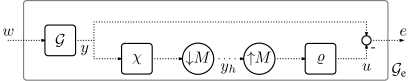
Figure 1: A setup for multi-rate discrete signal processing

Here, the input discrete signal ${y}$ is real and represented as the output of a system $\mathcal{G}$ driven by the discrete white Gaussian noise with zero mean. The transfer function (in $z$-domain) of $\mathcal{G}$ is represented by $G(z)$. Hence, the power spectral density of ${y}$ is given by $|G(\mathrm{e}^{\mathrm{j}\theta})|^{2}$ for all frequencies $\theta\in[-\pi,\pi]$. $\chi$ is the analysis filter whose output is down-sampled by a factor $M$. The down-sampled output is again upsampled by a factor $M$ followed by a synthesis filter $\varrho$. The reconstructed output ${u}$ is compared with the input signal ${y}$. The aim is to design both the analysis and synthesis filter given $G(z)$ in such a way that time averaged mean square error

$$J=\lim_{N\to\infty}\frac{1}{2N+1}\sum_{n=-N}^{N}E(e^{2}[n])$$

is minimised [9]. Here, $E$ is the expectation operator. Assume that the $\mathcal{G}$ is stable and $G(\mathrm{e}^{\mathrm{j}\theta})$ is dominant in the frequency band $[-\frac{\pi}{M},\frac{\pi}{M}]$ that means $|G(\mathrm{e}^{\mathrm{j}\theta_{1}})|>|G(\mathrm{e}^{\mathrm{j}\theta_{2}})|$ if $\theta_{1}\in[-\frac{\pi}{M},\frac{\pi}{M}]$ and $\theta_{2}\in[-\pi,\pi]\backslash[-\frac{\pi}{M},\frac{\pi}{M}]$. In this case, optimal synthesis and analysis filter give the error (see [9] for details)

$$J=\|\mathcal{G}\|_{{\textup{L}^{2}}}^{2}-\frac{1}{2\pi}\operatorname{tr}\int_{-\frac{\pi}{M}}^{\frac{\pi}{M}}G^{\sim}(\mathrm{e}^{\mathrm{j}\theta})G(\mathrm{e}^{\mathrm{j}\theta})\;d\theta.$$ (2)

Here, $\|\mathcal{G}\|_{{\textup{L}^{2}}}:=\|\mathcal{G}\|_{[-\pi,\pi]}$ represents the ${\textup{L}^{2}}$ norm of the system. Thus, we can see that truncated system norms naturally arises in multi-rate discrete signal processing. For a general $G(\mathrm{e}^{\mathrm{j}\theta})$, computation of (1) is needed [9].

It is further assumed that the discrete-time system $\mathcal{G}$ in (1) is linear discrete-time-invariant (LDTI) and its transfer function $G(z)$ is a proper rational transfer function with real coefficients. These type of systems can be represented in state space as $G(z)=D+C(zI-A)^{-1}B$ where $A,B,C$ and $D$ are real matrices. For simplicity of exposition, it is assumed that $D=0$ throughout this paper. It will be shown later in the paper that evaluation of the frequency truncated discrete-time system norm is a special case of the generalized problem of integration of a transfer function given in the descriptor form i.e

$$\int_{\theta_{1}}^{\theta_{2}}C(\mathrm{e}^{\mathrm{j}\theta}E-A)^{-1}B\;d\theta$$ (3)

where $A,B,C$, and $E$ are real matrices. The above integral is also helpful in the evaluation of the frequency-domain controllability and the observability Grammian of a system with transfer function $C(zI-A)^{-1}B$ [10, 5, 8, 2].

An expression for the frequency truncated discrete-time system norm for a stable discrete-time system is given in [8, Theorem 3.8] which depends upon invertibility of the $A$ matrix. This paper provides a modification which resolves this problem for a stable discrete-time system. This paper further generalizes the result of [8, Theorem 3.8] and provides an expression for (1) with minimal restriction on the system poles. Integral of a transfer function (of a discrete-time system) in the descriptor form and a numerically viable expression for its computation is also given in the paper. As a by-product, similar results for a continuous time system given in the descriptor form are briefly mentioned.

Section 2 contains an expression for the frequency truncated discrete-time system norm for a stable system and Section 3 contains an expression for the frequency truncated discrete-time system norm for a generic case. Integration of a transfer function given in the descriptor form is discussed in Section 3 and a method for its computation is given in Section 4. Section 5 contains results related to frequency truncated norm of a continuous time system given in the descriptor form.

Notation: $\mathbb{R}$ and $\mathbb{C}$ denote the set of real and complex numbers respectively. ${\bar{\mathbb{R}}^{-}}$ denotes the closed negative real axis (i.e. the negative real axis including zero). $\operatorname{Arg}(z)$ denotes the principal argument i.e. argument of the complex number $z$ in $(-\pi,\pi]$ and $\operatorname{wrap}(\theta):=\operatorname{Arg}(\mathrm{e}^{\mathrm{j}\theta})$ for all $\theta\in\mathbb{R}$. For square complex matrices $A$ and $E$, the matrix pencil $(A,E)$ is called regular if $\alpha E+\beta A$ is invertible for at-least one set of complex numbers $\alpha$ and $\beta$. An eigenvalue $\lambda\in\mathbb{C}$ of a matrix pencil $(A,E)$ satisfies $\det(A-\lambda E)=0$. We define $\mathrm{j}:=\sqrt{-1}$. $\sigma(A,E)$ denotes spectrum (the set of eigenvalues) of the matrix pencil $(A,E)$. A function $f$ is defined on $\sigma(A)$ if it follows definition $1.1$ of [3]. If $A\in\mathbb{C}^{n\times n}$ does not have any eigenvalues on the ${\bar{\mathbb{R}}^{-}}$ then there is a unique logarithm $Q=\log(A)$ whose all eigenvalues lie in the open horizontal strip $\{z\in\mathbb{C}|−\pi<\operatorname{imag}(z)<\pi\}$ of the complex plane [3, Theorem 1.31]. The $Q$ is known as the principal logarithm. The Fréchet derivative of a matrix function $f:\mathbb{C}^{n\times n}\to\mathbb{C}^{n\times n}$ at $A$ in the direction $X$ is denoted by $L_{f}(Q,X)$ [3, §3.1].

2 Stable Case

A discrete-time system $\mathcal{G}$ is defined stable if $A$ is Schur (i.e., all eigenvalues of $A$ are strictly inside the unit circle in the complex plane). It is well known that for a stable discrete-time system $\mathcal{G}$, the squared $L^{2}$ norm is given by

$$\|\mathcal{G}\|^{2}_{{\textup{L}^{2}}}:=\frac{1}{2\pi}\operatorname{tr}\int_{-\pi}^{\pi}G^{\sim}(\mathrm{e}^{\mathrm{j}\theta})G(\mathrm{e}^{\mathrm{j}\theta})\;d\theta=\operatorname{tr}B^{T}PB$$ (4)

where $P$ is the unique solution of the discrete Lyapunov equation

$$A^{T}PA-P+C^{T}C=0.$$ (5)

The frequency truncation discrete-time system norm can be calculated by evaluating an anti-derivative (or primitive) $\int G^{\sim}(\mathrm{e}^{\mathrm{j}\theta})G(\mathrm{e}^{\mathrm{j}\theta})\;d\theta$ first.

Theorem 2.1

Let discrete-time system $\mathcal{G}$ be stable and strictly proper and $G(\mathrm{e}^{\mathrm{j}\theta})=C(\mathrm{e}^{\mathrm{j}\theta}I-A)^{-1}B$ with A, B, C real matrices. Then, an anti-derivative $\int G^{\sim}(\mathrm{e}^{\mathrm{j}\theta})G(\mathrm{e}^{\mathrm{j}\theta})\;d\theta$ equals

$$B^{T}PB\theta+2\operatorname{imag}(B^{T}P\log(I-\mathrm{e}^{-\mathrm{j}\theta}A)B)$$

where $P$ is the unique solution of (5) and $\log$ denotes the principal logarithm and $\theta\in[-\pi,\pi]$.

• Consider function

  $$f(z,\theta)=\begin{cases}-\mathrm{j}z^{-1}\log(1-\mathrm{e}^{-\mathrm{j}\theta}z)&\text{if }z\neq 0\\ \mathrm{j}\mathrm{e}^{-\mathrm{j}\theta}&\text{if }z=0\end{cases}$$

  For a given $\theta\in[-\pi,\pi]$, $f(z,\theta)$ is analytic in the open unit disk around zero (in the complex plane) as $1-\mathrm{e}^{-\mathrm{j}\theta}z$ never lies on the closed negative real axis ${\bar{\mathbb{R}}^{-}}$. Clearly,

  $$\frac{\partial f(z,\theta)}{\partial\theta}=(\mathrm{e}^{\mathrm{j}\theta}-z)^{-1}$$

  is also analytic (for a given $\theta\in[-\pi,\pi]$) in the open unit disk around zero. Hence, it follows from [4, Theorem 6.2.27] that $f(A,\theta)$ is an anti-derivative of $(\mathrm{e}^{\mathrm{j}\theta}I-A)^{-1}$. Also, note that

  $$G^{\sim}(\mathrm{e}^{\mathrm{j}\theta}) G(\mathrm{e}^{\mathrm{j}\theta})=B^{T}(I-\mathrm{e}^{\mathrm{j}\theta}A^{T})^{-1}PB$$

  $$+B^{T}PA(\mathrm{e}^{\mathrm{j}\theta}I-A)^{-1}B$$

  $$= B^{T}PB+\mathrm{e}^{\mathrm{j}\theta}B^{T}(I-\mathrm{e}^{\mathrm{j}\theta}A^{T})^{-1}A^{T}PB$$

  $$+B^{T}PA(\mathrm{e}^{\mathrm{j}\theta}I-A)^{-1}B.$$

  Now, using the anti-derivative of $(\mathrm{e}^{\mathrm{j}\theta}I-A)^{-1}$ and the fact that integration (w.r.t. $\theta$) of the complex conjugate is the conjugate of integration, we have the result.         

The proof of the Theorem 2.1 is essentially similar to the proof of [8, Theorem 3.8] without the need for inversion of the $A$ matrix. Using [3, Theorem 1.31], we have

$$\|\mathcal{G}\|_{[-\pi,\pi]}^{2}=\operatorname{tr}B^{T}PB=\|\mathcal{G}\|_{{\textup{L}^{2}}}^{2}.$$

3 General case

In the previous section, the poles of a discrete-time system must be in the unit circle. We know that integration of a meromorphic function is possible as long as we are not integrating over a pole. Hence, systems with poles on the unit circle as well as inside and outside of the unit circle (apart from poles within the limits of integration) would be a more general case. This section is about the integration of a transfer function given in the descriptor form (see (3)) for the general case. This will further help in obtaining an expression for the frequency truncated discrete-time system norm in the general case. It is assumed that eigenvalue of the matrix pencil $(A,E)$ can lie on the unit circle as well as inside and outside of the unit circle. The result needs logarithm of matrices as expected. However, there are few mathematical technicalities which we have to take care.

The first issue is $\int(\mathrm{e}^{\mathrm{j}\theta}E-A)^{-1}\;d\theta$ is a function of two matrices $E$ and $A$. Hence, the definition of a matrix function given in [3] does not help here as it is. If $A$ or $E$ matrix is invertible then $\int(\mathrm{e}^{\mathrm{j}\theta}E-A)^{-1}\;d\theta$ can be written as a function of $EA^{-1}$ or $E^{-1}A$ respectively. However, the situation is a little complicated if both $E$ and $A$ are singular. Things can be simplified if we assume that the matrix pencil $(A,E)$ is regular. To illustrate this further, assume that the $(A,E)$ is regular and $\alpha\neq 0$ then

$$(zE-A)^{-1} =\alpha(\alpha E+\beta A)^{-1}(z(I-\beta Q)-\alpha Q)^{-1}$$

where $Q:=A(\alpha E+\beta A)^{-1}$. Hence, we need $\int\alpha(z(I-\beta Q)-\alpha Q)^{-1}\;d\theta$ which is a function of just one matrix $Q$. If $\alpha=0$ then $A$ is invertible. This case has been discussed already.

The second issue is related to the principal logarithm of a matrix as it does not exist if eigenvalues of the matrix lie on the closed negative real axis ${\bar{\mathbb{R}}^{-}}$. The critical task here is to choose the right anti-derivative of $\alpha(z(I-\beta Q)-\alpha Q)^{-1}$ such that the principal logarithm is defined. Furthermore, $Q$ can have eigenvalues on the unit circle as well as inside and outside of the unit circle. Hence, obtaining the right anti-derivative is quite challenging. For example, assume $\beta=0$, $\alpha=1$ and $A$ has at least one eigenvalue outside the unit circle. In this case, $Q=A$ and $\log(I-\mathrm{e}^{-\mathrm{j}\theta}A)$ (which we obtained in the stable case) is not a valid anti-derivative of $(zI-A)^{-1}$ as there exists a value of $\theta\in[-\pi,\pi]$ where eigenvalues of $I-\mathrm{e}^{-\mathrm{j}\theta}A$ lie on ${\bar{\mathbb{R}}^{-}}$. In this work, the right anti-derivative is obtained by the well-known tangent half-angle substitution i.e.

$$\mathrm{e}^{\mathrm{j}\theta}=\frac{1+\mathrm{j}t}{1-\mathrm{j}t}=-\frac{t-\mathrm{j}}{t+\mathrm{j}}$$ (6)

Here $t=\tan(\frac{\theta}{2})$. Selection of the right anti-derivative is also an issue in [7] which was solved by taking $\mathrm{j}$ out of the integrand whenever necessary. This technique is also used here along with the half-angle substitution.

Theorem 3.1

Assume that a discrete-time system $K$ can be represented in the descriptor form as $K(z)=(zE-A)^{-1}$ with real matrices $A$ and $E$. Also, assume that $\theta_{1},\theta_{2}\in(-\pi,\pi)$ and the matrix pencil $(A,E)$ is regular i.e. $W:=\alpha E+\beta A$ is invertible for at-least one set of complex numbers $\alpha$ and $\beta$. If $\mathrm{e}^{\mathrm{j}\phi}$ not an eigenvalue of $(A,E)$ for any $\phi\in\mathbb{R}$ and $\operatorname{wrap}(\phi)\in[\theta_{1},\theta_{2}]$ then

$$\int_{\theta_{1}}^{\theta_{2}}{K}(\mathrm{e}^{\mathrm{j}\theta})\;d\theta$$

$$=\lim_{\epsilon\to 0}\frac{1}{\mathrm{j}}A_{\epsilon}^{-1}\left(-\eta I+\log\left(\Gamma(\theta_{2},\epsilon)\Gamma(\theta_{1},\epsilon)^{-1}\right)\right)$$ (7a)

$$=\lim_{\epsilon\to 0}\frac{1}{\mathrm{j}}\left(-\eta I+\log\left(\Gamma(\theta_{1},\epsilon)^{-1}\Gamma(\theta_{2},\epsilon)\right)\right)A_{\epsilon}^{-1}$$ (7b)

where $A_{\epsilon}:=A+\alpha\epsilon I$, $E_{\epsilon}:=E-\beta\epsilon I$, $\epsilon\in\mathbb{C}$, $\eta:=\log\left(\frac{\tan(0.5\theta_{2})-\mathrm{j}}{\tan(0.5\theta_{1})-\mathrm{j}}\right)$ and $\Gamma(\theta,\epsilon):=(E_{\epsilon}+A_{\epsilon})\tan(0.5\theta)-\mathrm{j}(E_{\epsilon}-A_{\epsilon})$.

• Assume that $\alpha\neq 0$. Define

  $$f_{d}(z,\theta):=\begin{cases}\frac{1}{\mathrm{j}z}\left(-\eta+\log\frac{\Omega(z,t)}{\Omega(z,t_{1})}\right),&z\neq 0\\ \frac{\alpha}{\mathrm{j}}(\mathrm{e}^{-\mathrm{j}\theta_{1}}-\mathrm{e}^{-\mathrm{j}\theta})&z=0\end{cases}$$

  where $t:=\tan(\frac{\theta}{2})$ and $t_{1}:=\tan(\frac{\theta_{1}}{2})$ and $\Omega(z,t):=t(1-\beta z+\alpha z)-\mathrm{j}(1-\beta z-\alpha z)$ for a real $t$. If $z$ is an eigenvalue of $Q:=A(\alpha E+\beta A)^{-1}$ then $\frac{z\alpha}{1-\beta z}$ is also an eigenvalue of $(A,E)$. Hence, for all $\theta\in[\theta_{1},\theta_{2}]$, $f_{d}(z,\theta)$ is defined on $\sigma(Q)$ as long as $\mathrm{e}^{\mathrm{j}\phi}$ not an eigenvalue of $(A,E)$ for any $\operatorname{wrap}(\phi)\in[\theta_{1},\theta_{2}]$ (see Theorem A.1). Also,

  $$\frac{\partial f_{d}(z,\theta)}{\partial\theta} =\alpha\frac{1}{\mathrm{e}^{\mathrm{j}\theta}(1-\beta z)-\alpha z}.$$

  Now, it follows from Theorem A.2 and [4, Theorem 6.2.27] that $\int_{\theta_{1}}^{\theta_{2}}{K}(\mathrm{e}^{\mathrm{j}\theta})\;d\theta=W^{-1}\int_{\theta_{1}}^{\theta_{2}}\alpha(z(I-\beta Q)-\alpha Q)^{-1}\;d\theta=W^{-1}f_{d}(Q,\theta_{2})$. From [3, Theorem 3.8] and Theorem A.1, the Fréchet derivative $L_{f_{d}}(Q,X)$ of $f_{d}$ at $Q$ in the direction $X$ exists. Hence, $f_{d}(Q+\epsilon\alpha W^{-1})=f_{d}(Q)+\epsilon L_{f_{d}}(Q,\alpha W^{-1})+o(|\epsilon\alpha|\|W^{-1}\|)$. Hence, we have (7a). Equation (7b) follows from [3, Theorem 1.13.c].

  On the other hand, if $\alpha=0$ then $A$ is invertible and $\beta\neq 0$ by the regularity of $(A,E)$. Hence, $\int_{\theta_{1}}^{\theta_{2}}{K}(\mathrm{e}^{\mathrm{j}\theta})\;d\theta=A^{-1}\int_{\theta_{1}}^{\theta_{2}}(\mathrm{e}^{\mathrm{j}\theta}EA^{-1}-I)^{-1}\;d\theta$. Define for a complex $z$

  $$f_{i}(z,\theta):=\frac{1}{\mathrm{j}}\left(-\eta+\log\frac{t(z+1)-\mathrm{j}(z-1)}{t_{1}(z+1)-\mathrm{j}(z-1)}\right)$$

  where $t:=\tan(\frac{\theta}{2})$ and $t_{1}:=\tan(\frac{\theta_{1}}{2})$. If $z$ is an eigenvalue of $EA^{-1}$ then $\frac{1}{z}$ is an eigenvalue of $(A,E)$. Hence, for all $\theta\in[\theta_{1},\theta_{2}]$, $f_{i}(z,\theta)$ is defined on all eigenvalues of $EA^{-1}$ as long as $\mathrm{e}^{\mathrm{j}\phi}$ not an eigenvalue of $(A,E)$ for any $\operatorname{wrap}(\phi)\in[\theta_{1},\theta_{2}]$ (see Theorem A.2). Now, it follows from Theorem A.2 and [4, Theorem 6.2.27] that $\int_{\theta_{1}}^{\theta_{2}}{K}(\mathrm{e}^{\mathrm{j}\theta})\;d\theta=A^{-1}\int_{\theta_{1}}^{\theta_{2}}(\mathrm{e}^{\mathrm{j}\theta}EA^{-1}-I)\;d\theta=A^{-1}f_{i}(EA^{-1},\theta_{2})$. Equivalence to the limits can be proved in a manner similar the $\alpha\neq 0$ case.

          

Equation (7) can be extended for $\theta=\pi$ as shown in the following result.

Corollary 3.2

Let $k(z)$ be as in Theorem 3.1. Assume that $\theta_{1}\in(-\pi,\pi]$ and the matrix pencil $(A,E)$ is regular i.e. $W:=\alpha E+\beta A$ is invertible for at-least one set of complex numbers $\alpha$ and $\beta$. If $\mathrm{e}^{\mathrm{j}\phi}$ not an eigenvalue of $(A,E)$ for any $\phi\in\mathbb{R}$ and $\operatorname{wrap}(\phi)\in[\theta_{1},\pi]$ then $\int_{\theta_{1}}^{\pi}{K}(\mathrm{e}^{\mathrm{j}\theta})\;d\theta$ equals

$$\lim_{\epsilon\to 0}\frac{1}{\mathrm{j}}A_{\epsilon}^{-1}\left(\eta_{f}I-\log\left(t_{1}I-\mathrm{j}\Phi_{-}(\epsilon)\Phi_{+}(\epsilon)^{-1}\right)\right)$$

$$=\lim_{\epsilon\to 0}\frac{1}{\mathrm{j}}\left(\eta_{f}I-\log\left(t_{1}I-\mathrm{j}\Phi_{+}(\epsilon)^{-1}\Phi_{-}(\epsilon)\right)\right)A_{\epsilon}^{-1}$$ (8)

where $t_{1}:=\tan(\frac{\theta_{1}}{2})$, $A_{\epsilon}:=A+\alpha\epsilon I$, $E_{\epsilon}:=E-\beta\epsilon I$, $\epsilon\in\mathbb{C}$, $\eta_{f}:=\log(t_{1}-\mathrm{j})$, $\Phi_{+}(\epsilon)=E_{\epsilon}+A_{\epsilon}$ and $\Phi_{-}(\epsilon)=E_{\epsilon}-A_{\epsilon}$.

• Since $-1$ is not an eigenvalue of the matrix pencil $(A,E)$, $E+A$ is invertible. Define $t:=\tan(\frac{\theta}{2})$, $Q_{\epsilon}:=A_{\epsilon}W^{-1}$ and $\tilde{Q}:=(I-\beta Q_{\epsilon}-\alpha Q_{\epsilon})(I-\beta Q_{\epsilon}+\alpha Q_{\epsilon})^{-1}$. Now,

  $$\log\left(tI-\mathrm{j}(E_{\epsilon}-A_{\epsilon})(E_{\epsilon}+A_{\epsilon})^{-1}\right)=\log\left(tI-\mathrm{j}\tilde{Q}\right)$$

  For sufficiently small $|\epsilon|$, the above logarithm exits if $\mathrm{e}^{\mathrm{j}\phi}$ not an eigenvalue of $(A,E)$ for any $\phi\in\mathbb{R}$ and $\operatorname{wrap}(\phi)\in[\theta_{1},\pi]$ (the proof is similar to the proof Theorem A.1). Hence, [3, Theorem 11.3,Theorem 11.2] implies that

  $$\log\left(\frac{t-\mathrm{j}}{t_{1}-\mathrm{j}}\right) =\log(t-\mathrm{j})-\log(t_{1}-\mathrm{j})$$

  $$\log(Q_{t}) =\log(tI-\mathrm{j}\tilde{Q})-\log(t_{1}I-\mathrm{j}\tilde{Q}).$$

  where $Q_{t}:=(tI-\mathrm{j}\tilde{Q})(t_{1}I-\mathrm{j}\tilde{Q})^{-1}$. Now, using $\int_{\theta_{1}}^{\pi}{K}(\mathrm{e}^{\mathrm{j}\theta})\;d\theta=\lim_{\theta\to\pi}\int_{\theta_{1}}^{\theta_{2}}{K}(\mathrm{e}^{\mathrm{j}\theta})\;d\theta$ the result follows from [7, Lemma 5(2)].         

Similar results can be obtained if integral limits are $[-\pi,\theta_{1}]$ or $[-\pi,\pi]$. Note that if $A$ is invertible then (7) and (3.2) can be simplified by taking $\epsilon=0$. Otherwise, (7) and (3.2) needs a proper limit. Section 4 contains other forms of (7) and (3.2) which are independent of any limit. However, the current form is useful in obtaining a simple expression for the frequency truncated discrete-time system norm as explained in the following result.

Theorem 3.3

Suppose a discrete-time system $\mathcal{G}$ can be represented in state-space as $G(z)=C(zI-A)^{-1}B$ with real matrices A, B, and C. Define

$$A_{h} :=\begin{bmatrix}A&0\\ C^{T}C&I\end{bmatrix},\quad E_{h}:=\begin{bmatrix}I&0\\ 0&A^{T}\end{bmatrix},\quad$$

$$C_{h} :=\begin{bmatrix}0&-B^{T}\end{bmatrix},\quad\text{and}\quad B_{h}:=\begin{bmatrix}B\\ 0\end{bmatrix}.$$

Assume that $\theta_{1},\theta_{2}\in(-\pi,\pi)$. If $\mathrm{e}^{\mathrm{j}\phi}$ not an eigenvalue of $A$ for any $\phi\in\mathbb{R}$ such that $wrap(\phi)\in[\theta_{1},\theta_{2}]\cup[-\theta_{1},-\theta_{2}]$ then

$$\int_{\theta_{1}}^{\theta_{2}}G^{\sim}(\mathrm{e}^{\mathrm{j}\theta})G(\mathrm{e}^{\mathrm{j}\theta})\;d\theta=\frac{1}{\mathrm{j}}C_{h}\log\left(\Gamma_{d}(\theta_{1})^{-1}\Gamma_{d}(\theta_{2})\right)B_{h}$$

where $\Gamma_{d}(\theta):=(E_{h}+A_{h})\tan(0.5\theta)-\mathrm{j}(E_{h}-A_{h})$.

• The system $G^{\sim}(z)G(z)$ can be expressed as $G^{\sim}(z)G(z)=zC_{h}(zE_{h}-A_{h})^{-1}B_{h}$. Clearly,

  $$\int_{\theta_{1}}^{\theta_{2}}G^{\sim}(\mathrm{e}^{\mathrm{j}\theta})G(\mathrm{e}^{\mathrm{j}\theta})\;d\theta =\int_{\theta_{1}}^{\theta_{2}}C_{h}\left(E_{h}-\mathrm{e}^{-\mathrm{j}\theta}A_{h}\right)^{-1}B_{h}\;d\theta$$

  $$=\int_{-\theta_{1}}^{-\theta_{2}}C_{h}\left(\mathrm{e}^{\mathrm{j}\theta}A_{h}-E_{h}\right)^{-1}B_{h}\;d\theta$$

  Assume that $\lambda_{max}$ and $\lambda_{min}$ represents the maximum and minimum absolute values of eigenvalues of $A$. Now, $\det(E_{h}-\mu A_{n})=\det(I-\mu A)\det(A^{T}-\mu I)\neq 0$ if $\mu$ and $1/\mu$ is not an eigenvalue of $A$. Hence, the matrix pencil $(E_{h},A_{h})$ is regular. It also shows that the eigenvalues of $(E_{h},A_{h})$ are eigenvalues of $A$ and $A^{-1}$. This means, for any $\phi\in[\theta_{1},\theta_{2}]$, if $\mathrm{e}^{\mathrm{j}\phi}$ is not an eigenvalue of $(A_{h},E_{h})$ then $\mathrm{e}^{-\mathrm{j}\phi}$ not an eigenvalue of $(A_{h},E_{h})$. This implies $\mathrm{e}^{\mathrm{j}\phi}$ not an eigenvalue of $A$ for any $\phi\in[\theta_{1},\theta_{2}]\cup[-\theta_{1},-\theta_{2}]$. Note that $\lim_{\epsilon\to 0}(E_{h}+\epsilon\alpha I)^{-1}B_{h}=B_{h}$ and $C_{h}B_{h}=0$. Finally, equivalence to the limit needed in (7b) can be proved in a manner given in the proof of Theorem 3.1.         

Note that the above result does not need any limits.

4 Computation

Equation (7) can be converted into another form (independent of $\epsilon$) which uses exponential of matrices and

$$\psi_{1}(A):=\sum_{j=0}^{\infty}\frac{1}{(j+1)!}A^{j}$$ (9)

The advantage is that both of these functions have numerically accurate and reliable implementation [3, §10.5, §10.7.4].

Theorem 4.1

Let $\psi_{1}$ be as in (9). Using notations and conditions of Theorem 3.1, we have that $\int_{\theta_{1}}^{\theta_{2}}{K}(\mathrm{e}^{\mathrm{j}\theta})\;d\theta$ equals

$$\frac{1}{\mathrm{j}}W^{-1}\left(-\alpha L(\mathrm{e}^{-\mathrm{j}\theta_{2}}I-\mathrm{e}^{-\mathrm{j}\theta_{1}}\mathrm{e}^{Y})+\beta Y\right)$$ (10)

where $Y_{\epsilon}:=-\eta I+\log\left(\Gamma(\theta_{1},\epsilon)^{-1}\Gamma(\theta_{2},\epsilon)\right)$, $Y:=\lim_{\epsilon\to 0}Y_{\epsilon}=-\eta I+\log\left(\Gamma(\theta_{2},0)\Gamma(\theta_{1},0)^{-1}\right)$ and $L:=\lim_{\epsilon\to 0}(\mathrm{e}^{Y_{\epsilon}}-I)^{-1}Y_{\epsilon}=\psi_{1}(Y)^{-1}$.

• $Y=\lim_{\epsilon\to 0}Y_{\epsilon}$ due to Theorem A.1.

Note that

$$(E_{\epsilon}+A_{\epsilon})t-\mathrm{j}(E_{\epsilon}-A_{\epsilon})=(t-\mathrm{j})(E_{\epsilon}-\mathrm{e}^{-\mathrm{j}\theta}A_{\epsilon})$$ (11)

where $t:=\tan(\frac{\theta}{2})$. Now,

$$\exp\left(-\eta I+\log\left(\Gamma(\theta_{2},\epsilon)\Gamma(\theta_{1},\epsilon)^{-1})\right)\right)=\mathrm{e}^{Y_{\epsilon}}.$$

Using [3, Theorem 10.2,Theorem 1.17], we have

$$\frac{t_{1}-\mathrm{j}}{t_{2}-\mathrm{j}}\left(\Gamma(\theta_{2},\epsilon)\Gamma(\theta_{1},\epsilon)^{-1})\right)=\mathrm{e}^{Y_{\epsilon}}$$

where $t_{i}:=\tan(\frac{\theta_{i}}{2})$. Assume $\alpha\neq 0$. Using (11), we have

$$\alpha(1-\mathrm{e}^{Y_{\epsilon}})E_{\epsilon}W^{-1} =\alpha(\mathrm{e}^{-\mathrm{j}\theta_{2}}I-\mathrm{e}^{-\mathrm{j}\theta_{1}}\mathrm{e}^{Y_{\epsilon}})A_{\epsilon}W^{-1}$$

$$(1-\mathrm{e}^{Y_{\epsilon}})\alpha(E-\beta\epsilon I)W^{-1} =\alpha MA_{\epsilon}W^{-1}$$

where $W:=\alpha E+\beta A$ and $M_{\epsilon}:=\mathrm{e}^{-\mathrm{j}\theta_{2}}I-\mathrm{e}^{-\mathrm{j}\theta_{1}}\mathrm{e}^{Y_{\epsilon}}$. Further, simplifying using $\alpha EW^{-1}=I-\beta AW^{-1}$, $Q_{\epsilon}:=A_{\epsilon}W^{-1}=AW^{-1}+\alpha\epsilon W^{-1}$ and $\alpha E_{\epsilon}W^{-1}:=I-\beta Q_{\epsilon}$, we have $I-\mathrm{e}^{Y_{\epsilon}}=(\alpha M_{\epsilon}+(I-\mathrm{e}^{Y_{\epsilon}})\beta)Q_{\epsilon}$. Using [3, Theorem 1.13.a] and

$$\int_{\theta_{1}}^{\theta_{2}}K(\mathrm{e}^{\mathrm{j}\theta})d\theta=\lim_{\epsilon\to 0}\frac{1}{\mathrm{j}}W^{-1}Q_{\epsilon}^{-1}Y_{\epsilon},$$

we have the result. Equivalence of $L$ and $\psi$ is standard [3, §10.7.4]. Note that $L$ is invertible because it has no zero eigenvalues.

If $\alpha=0$ then $A$ is invertible and $\beta\neq 0$ by the regularity of $(A,E)$. Hence, $\int_{\theta_{1}}^{\theta_{2}}{K}(\mathrm{e}^{\mathrm{j}\theta})\;d\theta=\frac{1}{\mathrm{j}}A^{-1}Y$.         

Equation (3.2) can be also modified in a manner similar to Theorem 4.1.

Corollary 4.2

Let $\psi_{1}$ be as in (9). Using notations and conditions of Corollary 3.2, we have that

$$\int_{\theta_{1}}^{\pi}{K}(\mathrm{e}^{\mathrm{j}\theta})\;d\theta =\frac{1}{\mathrm{j}}W^{-1}L_{f}\left(\mathrm{e}^{Y}(\alpha-\beta)+(\mathrm{e}^{-\mathrm{j}\theta_{1}}\alpha+\beta)I\right)$$

where $Y_{\epsilon}:=-\eta_{f}I+\log\left(tI-\mathrm{j}\Phi_{-}(\epsilon)\Phi_{+}(\epsilon)^{-1}\right)$, $Y:=\lim_{\epsilon\to 0}Y_{\epsilon}=-\eta_{f}I+\log\left(tI-\mathrm{j}\Phi_{-}(0)\Phi_{+}(0)^{-1}\right)$ and $L_{f}:=\lim_{\epsilon\to 0}(\mathrm{e}^{Y_{\epsilon}}-I)^{-1}Y_{\epsilon}=\psi_{1}(Y)$.

5 A brief note on the continuous time system

Similar to Theorem 3.1 and Theorem 4.1, the results of [7] can be extended to the continuous time descriptor systems. These results are useful in the model reduction applications [6]. The proof is similar to Theorem 3.1 and Theorem 4.1.

Theorem 5.1

Let $\psi_{1}$ be as in (9). Assume that a continuous time system $K$ can be represented in the descriptor form as $K(s)=(sE-A)^{-1}$ with real matrices $A$ and $E$. Also, assume that $\omega_{1},\omega_{2}\in\mathbb{R}$ and the matrix pencil $(A,E)$ is regular i.e. $W:=\alpha E+\beta A$ is invertible for at-least one set of complex numbers $\alpha$ and $\beta$. If the matrix pencil $(A,E)$ has no imaginary eigenvalue $\mathrm{j}\lambda$ with $\lambda\in[\omega_{1},\omega_{2}]$ then

$$\int_{\omega_{1}}^{\omega_{2}}{K}(\mathrm{j}\omega)\;d\omega =\lim_{\epsilon\to 0}\frac{1}{\mathrm{j}}E_{\epsilon}^{-1}\log\left(\tilde{\Omega}(\omega_{2},\epsilon)\tilde{\Omega}(\omega_{1},\epsilon)^{-1}\right)$$

$$=\lim_{\epsilon\to 0}\frac{1}{\mathrm{j}}\log\left(\tilde{\Omega}(\omega_{1},\epsilon)^{-1}\tilde{\Omega}(\omega_{2},\epsilon)\right)E_{\epsilon}^{-1}$$

$$=-W^{-1}\left(\beta\tilde{L}(\omega_{2}I-\mathrm{e}^{\tilde{Y}}\omega_{1})+\mathrm{j}\alpha\tilde{Y}\right)$$

where $A_{\epsilon}:=A+\alpha\epsilon I$, $E_{\epsilon}:=E-\beta\epsilon I$, $\epsilon\in\mathbb{C}$, $\tilde{\Omega}(\omega,\epsilon):=\omega E_{\epsilon}+\mathrm{j}A_{\epsilon}$, $\tilde{Y}_{\epsilon}:=\log\left(\tilde{\Omega}(\omega_{2},\epsilon)\tilde{\Omega}(\omega_{1},\epsilon)^{-1}\right)$ $\tilde{Y}:=\lim_{\epsilon\to 0}\tilde{Y}_{\epsilon}=\log\left(\tilde{\Omega}(\omega_{2},0)\tilde{\Omega}(\omega_{1},0)^{-1}\right)$ and $\tilde{L}:=\lim_{\epsilon\to 0}(\mathrm{e}^{\tilde{Y}_{\epsilon}}-1)^{-1}\tilde{Y}_{\epsilon}=\psi_{1}(\tilde{Y})^{-1}$.

6 Conclusions

Computation of the frequency truncated discrete-time system norm arises in different signal processing and model reduction applications. This paper contains expressions for integral of the transfer function of a discrete-time system given in the descriptor form. The result for the descriptor system is used in obtaining the frequency truncated norm of a discrete-time system in the general case. Simplified results in case of stable systems are also given in the paper. Similar results for the continuous time systems given in the descriptor form, are also mentioned briefly.

Appendix A Appendix

The results in this section explain when the functions required in the proof of Theorem 3.1 are defined. Note that an analytic function in domain $D$ is always defined at all $z\in D$.

Theorem A.1

Let $\alpha$ and $\beta$ be any two complex numbers and $\theta_{1},\theta\in(-\pi,\pi)$. Define a complex function

$$f_{d}(z,\theta):=\begin{cases}\frac{1}{\mathrm{j}z}\left(-\eta+\log\frac{\Omega(z,t)}{\Omega(z,t_{1})}\right),&z\neq 0\\ \frac{\alpha}{\mathrm{j}}(\mathrm{e}^{-\mathrm{j}\theta_{1}}-\mathrm{e}^{-\mathrm{j}\theta})&\text{elsewhere}\end{cases}$$

where $\eta:=\log\left(\frac{\tan(0.5\theta)-\mathrm{j}}{\tan(0.5\theta_{1})-\mathrm{j}}\right)$, $t:=\tan(\frac{\theta}{2})$ and $t_{1}:=\tan(\frac{\theta_{1}}{2})$ and $\Omega(z,t):=t(1-\beta z+\alpha z)-\mathrm{j}(1-\beta z-\alpha z)$ for a real $t$. Assume that $\alpha\neq 0$. Then, $f_{d}(z,\theta)$ is analytic in $\mathbb{C}\backslash\hat{D}$ where $\hat{D}:=\{z\in\mathbb{C}|\frac{\alpha z}{1-\beta z}=\mathrm{e}^{\mathrm{j}\theta},\operatorname{wrap}(\phi)\in[\theta_{1},\theta]\}$. Here, $\mathbb{C}\backslash\hat{D}$ is an open set.

• It is straightforward to verify that $\eta$ is well defined.

It is now shown that $\mathbb{C}\backslash\hat{D}$ is an open set. Assume $\beta=0$, then the result is trivial. Assume $\beta\neq 0$ then $g(z):=\frac{\alpha z}{1-\beta z}$ is continuous apart from the point $z=\frac{1}{\beta}$. Since the set $Y:=\{\mathrm{e}^{\mathrm{j}\phi}|\phi\in[\theta_{1},\theta]\}$ is closed and $g^{-1}(Y)$ does not contain $z=\frac{1}{\beta}$, continuity of $g$ in $\mathbb{C}\backslash\{0\}$ implies that $\mathbb{C}\backslash\hat{D}$ is an open set.

To check whether $\log\frac{\Omega(z,t)}{\Omega(z,t_{1})}$ is well defined or not, first assume that $1-\beta z\neq 0$. Then, $\Omega(z,t_{1})=(t_{1}+\mathrm{j})(-\mathrm{e}^{\mathrm{j}\theta_{1}}(1-\beta z)+\alpha z)$. Hence, $\Omega(z,t_{1})$ is invertible as $z\notin\hat{D}$. Assume that the principal log does not exist for a $z\notin\hat{D}$. This means

$$\log\frac{\Omega(z,t)}{\Omega(z,t_{1})} =\frac{t(1+a)-\mathrm{j}(1-a)}{t_{1}(1+a)-\mathrm{j}(1-a)}=-\rho$$

for all $\rho\geq 0$. Here, $a:=\frac{\alpha z}{1-\beta z}$. The above implies that $a$ must be on unit circle i.e. $a=\mathrm{e}^{\mathrm{j}\psi}$. If $a=-1$ (i.e. $\psi=\pi$) then it is trivial to see that the principal log exist. On the other hand if $a=\mathrm{e}^{\mathrm{j}\psi}$ and $a\neq-1$ then

$$\frac{(1+a)t-\mathrm{j}(1-a)}{(1+a)t_{1}-\mathrm{j}(1-a)} =\frac{t-\tan{\frac{\psi}{2}}}{t_{1}-\tan{\frac{\psi}{2}}}=-\rho$$

iff $\tan{\frac{\psi}{2}}=\frac{\rho t_{1}+t}{\rho+1}$. This means $\psi\in[\theta_{1},\theta]$. Hence, $z\in\hat{D}$. Contradiction. Therefore, the principal log exists for all $z\notin\hat{D}$.

Now, assume $1-\beta z=0$. Then, $\beta\neq 0$, $z\neq 0$ and $\Omega(z,t_{1})=(t_{1}+\mathrm{j})\alpha z$. Hence, $\Omega(z,t_{1})$ is invertible as $\alpha\neq 0$. Also, $\log\frac{\Omega(z,t)}{\Omega(z,t_{1})}=\log(\frac{t+\mathrm{j}}{t_{1}+\mathrm{j}})$. It is straightforward to see that this logarithm exists.

The above analysis implies that $\frac{1}{\mathrm{j}z}\left(-\eta+\log\frac{\Omega(z,t)}{\Omega(z,t_{1})}\right)$ is analytic on an open set $\mathbb{C}\backslash\hat{D}$ apart from $z=0$ where it has a removable singularity. Clearly, $\lim_{z\to 0}f_{d}(z,\theta)=f_{d}(0,\theta)$. Hence, $f_{d}(z,\theta)$ is analytic in $\mathbb{C}\backslash\hat{D}$ (see e.g. [1, §16.20]).         

The proof of the following result is similar to the proof of Theorem A.1.

Theorem A.2

Let $\eta$ be as in Theorem A.1 and $\theta_{1},\theta\in(-\pi,\pi)$. Define a complex function

$$f_{i}(z,\theta):=\frac{1}{\mathrm{j}}\left(-\eta+\log\frac{t(z+1)-\mathrm{j}(z-1)}{t_{1}(z+1)-\mathrm{j}(z-1)}\right)$$

where $t:=\tan(\frac{\theta}{2})$ and $t_{1}:=\tan(\frac{\theta_{1}}{2})$. Now, $f_{i}(z,\theta)$ is analytic in $\mathbb{C}\backslash\tilde{D}$ where $\tilde{D}:=\{\mathrm{e}^{-\mathrm{j}\phi}|\operatorname{wrap}(\phi)\in[\theta_{1},\theta]\}$. Here, $\mathbb{C}\backslash\hat{D}$ is an open set.

References

• [1] T.M. Apostol. Mathematical Analysis. Addison-Wesley, 1974.
• [2] A.Β Ghafoor and V.Β Sreeram. Model reduction via limited frequency interval gramians. IEEE Transactions on Circuits and Systems I: Regular Papers, 55:2806 – 2812, 11 2008.
• [3] N.J. Higham. Functions of Matrices: Theory and Computation. SIAM, 2008.
• [4] R.A. Horn and C.R. Johnson. Topics in Matrix Analysis. Cambridge University Press, 1991.
• [5] L.G. Horta, J.Β Juang, and R.W. Longman. Discrete-time model reduction in limited frequency ranges. Journal of Guidance, Control and Dynamics, 16(6):1125–1130, 1993.
• [6] M.Β Imran and A.Β Ghafoor. Model reduction of descriptor systems using frequency limited gramians. Journal of the Franklin Institute, 352(1):33–51, 2015.
• [7] G.Β Meinsma and H.Β S. Shekhawat. Frequency-truncated system norms. Automatica, 47(8):1842 – 1845, 2011.
• [8] D.Β Petersson. A Nonlinear Optimization Approach to $H_{2}$-Optimal Modeling and Control. PhD thesis, LinkΓΆping University, 2013.
• [9] M.K. Tsatsanis and G.B. Giannakis. Principal component filter banks for optimal multiresolution analysis. IEEE Transaction Signal Processing, 43(8):1766 –1777, aug 1995.
• [10] D.Β Wang and A.Β Zilouchian. Model reduction of discrete linear systems via frequency-domain balanced structure. IEEE Transactions on Circuits and Systems I: Fundamental Theory and Applications, 47:830 – 837, 07 2000.