Spectral Calibration of K $-$ M Giants from medium resolution near-infrared HK-band spectra

Supriyo Ghosh,¹ Soumen Mondal,¹ Ramkrishna Das¹ and Dhrimadri Khata¹
¹Satyendra Nath Bose National Centre for Basic Sciences, Block-JD, Sector-III, Salt Lake, Kolkata-700 106, India
E-mail: supriyo12a@bose.res.in (SG)

(Accepted 2019 January 23. Received 2019 January 23; in original form 2018 August 29)

Abstract

We present here new medium resolution spectra ( $\lambda/\Delta\lambda$ $\sim$ 1200) of K $-$ M giants covering wavelength range 1.50 $-$ 1.80 and 1.95 $-$ 2.45 $\mu$ m. The sample includes 72 K0 $-$ M8 giants from our TIRSPEC observations and all available 35 giants in that spectral range from archival IRTF spectral library. We have calibrated here the empirical relations between fundamental parameters (e.g., effective temperature, surface gravity) and equivalent widths of some important spectral features like Si I, Na I, Ca I, ¹²CO. We find that the ¹²CO first overtone band at 2.29 $\mu$ m and second overtone band at 1.62 $\mu$ m are a reasonably good indicator of temperature above 3400 K and surface gravity. We show that the dispersion of empirical relations between ¹²CO and $T_{eff}$ significantly improve considering the effect of surface gravity.

keywords:

stars: fundamental parameters – infrared: stars – techniques: spectroscopic – methods: observational

^†^†pubyear: 2017^†^†pagerange: Spectral Calibration of K

-

M Giants from medium resolution near-infrared HK-band spectra–A

1 Introduction

Stellar spectral libraries have a particularly important role to understand and classify the stellar population as well as an evolutionary synthesis for the individual sources in the field, star clusters of our Galaxy and integrated stellar lights in the extra-Galactic sources. For example, the original stellar classification process, developed by Morgan et al. (1943), uses a set of reference stellar spectra to compare the spectrum of an individual star (see Garrison 1994). Precise estimation of their fundamental parameters, e.g., effective temperature ( $T_{eff}$ ), surface gravity (log $g$ ), metallicity [Fe/H], mass (M), and radius (r), from spectroscopic techniques is still challenging.

Several optical spectral libraries (e.g., ELODIE (Prugniel & Soubiran, 2001), STELIB (Le Borgne et al., 2003), CFLIB (Valdes et al., 2004), Indo-US (Valdes et al., 2004), MILES (Sánchez-Blázquez et al., 2006), CaT (Cenarro et al., 2001, 2007)) are used to construct reasonable stellar population models. The near-infrared (NIR) spectral regions are more advantageous than optical as it suffers relatively less interstellar extinction, and the NIR regime allows us to probe long distance in the galaxy. NIR spectra are particularly useful for understanding the physics of cool stars like K $-$ M giants (e.g., Joyce et al. 1998; Gautschy-Loidl et al. 2004) as these cool stars ( $T_{eff}\sim 3000-6000$ ) emit maximum energy (peak near 1 $\mu$ m) in the NIR, which can probe the deepest regions of the stellar photosphere (Förster Schreiber, 2000). Particularly, classifying and characterizing of individual stars in nearby embedded young clusters (e.g., Greene & Meyer 1995; Peterson et al. 2008) and optically obscured regions of the Galaxy (e.g., Figer et al. 1995; Frogel et al. 2001; Kurtev et al. 2007; Lançon et al. 2007; Riffel et al. 2008) are much benefited by the use of NIR spectra.

Since the pioneering work of Johnson & Méndez (1970), significant progress was made by several authors in the NIR regions (see, e.g., Origlia et al. 1993; Wallace & Hinkle 1997; Meyer et al. 1998 for reviews). Subsequently, several spectral libraries have been developed to construct stellar population synthesis models from NIR spectra (e.g., Kleinmann & Hall 1986; Terndrup et al. 1990; Origlia et al. 1993; Wallace & Hinkle 1996, 1997, 2002; Blum et al. 1996; Joyce et al. 1998; Förster Schreiber 2000; Lançon & Wood 2000; Ivanov et al. 2004; Mármol-Queraltó et al. 2008; Rayner et al. 2009; Chen et al. 2014; Feldmeier-Krause et al. 2017; Villaume et al. 2017). Among those libraries, the NASA Infrared Telescope Facility (IRTF) spectral library offers a unique advantage of continuous coverage in the NIR and mid-IR (MIR) regime (0.8 $-$ 5 $\mu$ m) but provides limited coverage of stellar parameter range (Cushing et al., 2005; Rayner et al., 2009). The X-Shooter stellar library (Chen et al., 2014) that covers optical to near-IR (0.35 $-$ 2.5 $\mu$ m) would be beneficial once it is complete. Moreover, ongoing large-scale spectroscopic surveys like, Sloan Extension for Galactic Understanding and Exploration (SEGUE; Yanny et al. 2009), the Radial Velocity Experiment (Steinmetz et al., 2006), the Apache Point Observatory Galactic Evolution Experiment (Eisenstein et al., 2011), the LAMOST Spectroscopic Survey of the Galactic Anti-center (LSS-GAC; Liu et al. 2014; Yuan et al. 2015) and Gaia (Perryman et al., 2001), will be valuable for our understanding about the formation and evolution of the Milky Way.

Despite all these efforts in the understanding of stellar population in different systems, precise estimation of fundamental parameters of cool giants still remains a challenge because of their molecular near-photospheric environment (Lançon & Wood, 2000). The spectral database of these cool giants is highly sparse, and more additional database would be highly valuable for their classification and characterization. Furthermore, the understanding of quantitative diagnostic tools and quality of spectral indices have an important role to quantify the stellar absorption features. In this paper a new NIR stellar spectral library of K $-$ M giants has been undertaken using the medium resolution spectra ( $\lambda/\Delta\lambda$ $\sim$ 1200) covering the wavelength range 1.50 $-$ 2.45 $\mu$ m. The main motivation of the present work is to widen the existing cool stellar libraries, and more importantly, investigate how accurately the fundamental parameters (e.g., T_eff and log $g$ ) can be estimated from the medium-resolution NIR HK-band spectra. In addition, the present work evaluates the systematic differences between our established relations in this paper and the existing relations in the literature derived from relatively high-resolution spectra. Particularly, the present calibration could be used to derive the fundamental parameters for relatively faint sources in the high-extinction regions from such medium-resolution spectra compared to higher-resolution spectra using big aperture telescopes. Moreover, the estimation of fundamental parameters of K- and M-giants, precisely later than M3, is still a challenging task, and none of the existing libraries contains a large sample of later M3 giants for such calibrations. The paper is organized as the details of our observations and data reduction procedures are described in section 2, section 3 presents different spectral analysis tools, and section 4 deals with our new results and discussion. Finally, the summary and conclusion of our studies are presented in section 5.

2 Observations and Data reductions

Table 1: Identification of Stars observed with TIRSPEC and SpeX instruments

Stars	V	ST	$T_{eff}$	log $g$	[Fe/H]	Parallax	Date Of	Exposure	SNR $\ddagger$	Sky	Ref
Names	mag		(K)	(cm/ $s^{2}$ )	(dex)	(mas)	Observation	Time (s) $\dagger$		Conditions
TIRSPEC :
HD54810	4.92	K0III	4715	2.395	-0.25	16.08	2014-12-12	2(560)	138	clear sky	T1,M1
HD99283	5.70	K0III	4874	2.476	-0.18	10.63	2017-04-09	2(3100)	181	clear sky	T1,M2
HD102224	3.72	K0III	4482	1.844	-0.33	17.76	2015-01-17	2(517)	171	clear sky	T1,M5
HD69994	5.79	K1III	4571	2.157	-0.07	5.79	2017-04-07	2(580)	144	clear sky	T1,M2
HD40657	4.52	K1.5III	4400	1.389	-0.58	7.75	2014-12-12	2(525)	130	clear sky	T1,M2
HD85503	3.88	K2III	4504	2.306	0.25	26.28	2015-01-14	2(540)	116	clear sky	T1,M1
HD26846	4.86	K2III	4547	2.125	0.09	13.46	2014-12-12	2(550)	106	clear sky	T1,M6
HD30834	4.77	K3III	4096	0.925	-0.24	5.42	2015-01-13	2(540)	164	clear sky	T1,M5
HD92523	4.99	K3III	4115	1.349	-0.38	7.81	2015-01-17	2(532)	240	clear sky	T1,M2
HD97605	5.79	K3III	4606	2.701	–	16.51	2017-04-09	2(380)	130	clear sky	T1
HD49161	4.77	K4III	4243	1.212	-0.03	6.62	2014-12-12	2(530)	121	clear sky	T1,M2
HD70272	4.25	K4+III	3900	0.914	-0.24	8.53	2015-01-17	2(58)	174	clear sky	T1,M9
HD99167	4.80	K5III	3865	1.133	-0.06	8.67	2015-01-14	2(530)	153	clear sky	T1, M10
HD83787	5.84	K6III	3816	0.892	-0.21	4.22	2015-01-14	2(570)	117	clear sky	T1,M7
HD6953	5.79	K7III	4021	1.662	–	8.28	2014-12-12	2(650)	103	clear sky	T1
HD6966	6.04	M0III	3998	1.483	–	6.06	2015-12-18	2(340)	144	clear sky	T1
HD18760	6.13	M0III	3605	0.569	–	3.92	2016-12-20	2(530)	133	clear sky	T1
HD38944	4.74	M0III	3799	0.727	–	6.24	2015-01-14	2(525)	95	clear sky	T1
HD60522	4.06	M0III	3881	1.110	-0.36	12.04	2014-12-12	2(57)	79	thin cloud	T1,M9
HD216397	4.93	M0III	3889	1.352	–	10.03	2015-08-11	2(330)	117	thin cloud	T1
HD7158	6.11	M1III	3747	0.700	–	5.16	2015-12-18	2(330)	123	clear sky	T1
HD82198	5.37	M1III	3875	1.153	–	6.80	2015-01-14	2(340)	101	clear sky	T1
HD218329	4.52	M1III	3874	1.123	0.17	9.92	2015-08-11	2(315)	86	thin cloud	T1,M5
HD219215	4.22	M1III	4307	1.749	–	16.14	2015-08-11	2(67)	71	thin cloud	T1
HD119149	5.01	M1.5III	3675	0.714	–	6.40	2015-01-14	2(530)	94	clear sky	T1
HD1013	4.80	M2III	3792	1.028	–	8.86	2015-12-18	2(37)	131	clear sky	T1
HD33463	6.42	M2III	3491	0.299	-0.05	3.11	2015-01-14	2(530)	115	clear sky	T1, M3
HD39732	7.43	M2III	3448	0.380	–	2.42	2016-12-19	2(525)	111	clear sky	T1
HD43151	8.49	M2III	3335	0.231	–	1.99	2016-12-19	2(530)	170	clear sky	T1
HD92620	6.02	M2III	3500	–	–	4.02	2016-12-19	2(520)	182	clear sky	T1
HD115521	4.80	M2III	3690	0.418	–	4.83	2015-01-17	2(47)	142	clear sky	T1
HD16058	5.37	M3III	3572	0.489	0.08	5.16	2015-01-13	2(520)	94	clear sky	T1, M11
HD28168	8.42	M3III	3344	0.497	–	2.77	2015-01-13	2(560)	83	clear sky	T1
HD66875	5.99	M3III	3509	0.441	–	4.38	2016-12-19	2(512)	143	clear sky	T1
HD99056	8.79	M3III	3137	0.439	–	4.52	2016-12-19	2(56)	119	clear sky	T1
HD215953	6.84	M3III	3460	0.823	–	4.17	2015-08-11	2(3100)	80	thin cloud	T1
HD223637	5.78	M3III	3622	0.567	–	3.86	2015-12-19	2(315)	125	clear sky	T1
HD25921	7.10	M3/M4III	3522	0.721	–	3.62	2016-12-20	2(540)	110	clear sky	T1
HD33861	8.64	M3.5III	3365	0.565	–	2.49	2015-01-13	2(570)	115	clear sky	T1
HD224062	5.61	M3/M4III	3429	0.299	–	5.12	2015-12-19	2(35)	93	clear sky	T1
HD5316	6.24	M4III	3481	0.693	–	5.75	2015-12-18	2(310)	129	clear sky	T1
HD34269	5.65	M4III	3427	0.353	–	5.79	2015-01-13	2(510)	141	clear sky	T1
HD64052	6.39	M4III	3460	0.783	–	6.45	2016-12-19	2(510)	84	clear sky	T1
HD81028	6.89	M4III	3482	0.147	–	2.08	2016-12-19	2(520)	135	clear sky	T1
HD206632	6.23	M4III	3367	0.195	–	4.77	2015-08-11	2(35)	73	thin cloud	T1
HD16896	8.25	M5III	3358	0.360	–	2.68	2016-12-20	2(530)	123	clear sky	T1
HD17491	6.90	M5III	3313	0.071	–	3.90	2016-12-20	2(56)	107	clear sky	T1

V mag $-$ visual magnitude, ST $-$ spectral type, T_eff $-$ effective temperature, log $g$ $-$ surface gravity, [Fe/H] $-$ metallicity
$\dagger$ Exposure Time = no. of dither position*(no. of frame in each dither position* integration time)
$\ddagger$ SNR $-$ signal to noise ratio, are estimated by the method as in Stoehr et al. (2008) considering the whole H-band.
Ref $-$ references of $T_{eff}$ , log $g$ and [Fe/H]. T corresponds to the reference of $T_{eff}$ and log $g$ ; M corresponds to the reference of [Fe/H]
Ref : (T1) McDonald et al. (2017); (T2) McDonald et al. (2012) ; (T3) Wright et al. (2003); (T4, M4) Cesetti et al. (2013) ; (T5, M5) Prugniel et al. (2011);
(M1) Jofré et al. (2015); (M2) Soubiran et al. (2016); (M3) Ho et al. (2017); (M6) Massarotti et al. (2008); (M7) Wu et al. (2011); (M8) McWilliam (1990); (M9) Reffert et al. (2015); (M10) Gáspár, Rieke & Ballering (2016); (M11) Boeche, Smith & Grebel et al. (2018); (M12) Luck & Heiter (2007); (M13) Luo et al. (2016)
V mag, ST, Parallax are taken from SIMBAD

Table 2: continued

Stars	V	ST	$T_{eff}$	log $g$	[Fe/H]	Parallax	Date Of	Exposure	SNR	Sky	Ref
Names	mag		(K)	(cm/ $s^{2}$ )	(dex)	(mas)	Observation	Time (s)		Conditions
HD17895	7.16	M5III	3294	-0.021	–	2.72	2016-12-20	2(57)	120	clear sky	T1
HD22689	7.16	M5III	3144	-0.135	–	3.85	2015-12-18	2(34)	77	clear sky	T1
HD26234	8.90	M5III	3191	0.390	–	2.95	2015-01-13	2(550)	94	clear sky	T1
HD39983	8.26	M5III	3145	0.430	-0.23	4.73	2016-12-19	2(510)	154	clear sky	T1,M3
HD46421	8.21	M5III	3225	0.215	–	3.57	2016-12-19	2(510)	114	clear sky	T1
HD66175	7.04	M5III	3156	0.158	–	3.41	2015-01-17	2(512)	128	clear sky	T1
HD103681	6.20	M5III	3215	-0.056	–	2.81	2016-12-19	2(550)	124	clear sky	T1
HD105266	7.18	M5III	3246	0.001	–	3.69	2015-01-14	2(510)	83	clear sky	T1
HD64657	6.85	M5/M6III	3269	0.031	–	3.78	2016-12-19	2(56)	114	clear sky	T1
HD65183	6.40	M5/M6III	3359	0.020	–	2.93	2016-12-19	2(56)	94	thin cloud	T1
HD223608	8.86	M5/M6III	3228	–	–	0.57	2015-12-19	2(315)	136	clear sky	T2
HD7861	8.54	M6III	3259	–	–	4.20	2015-01-13	2(540)	100	clear sky	T2
HD18191	5.93	M6III	3336	0.332	-0.24	9.28	2015-12-18	2(34)	98	clear sky	T1,M5
HD27957	8.03	M6III	3383	0.298	–	2.38	2016-12-20	2(540)	127	clear sky	T1
HD70421	8.55	M6III	3120	-0.112	–	2.22	2016-12-19	2(512)	104	clear sky	T1
HD73844	6.67	M6III	3206	0.109	–	6.40	2015-12-18	2(35)	87	clear sky	T1
HIP44601	9.20	M6III	3200	–	–	1.25	2015-03-02	2(550)	151	clear sky	T2
HIC55173	7.42	M6III	3288	0.280	–	4.48	2016-12-19	2(510)	134	clear sky	T1
HIP57504	8.74	M6III	2920	0.011	–	3.86	2016-12-19	2(510)	150	clear sky	T1
HD115322	7.21	M6III	3458	–	–	1.3	2015-01-16	2(535)	97	clear sky	T2
HD203378	7.32	M6III	3284	0.035	–	3.23	2015-08-11	2(320)	57	clear sky	T1
HD43635	7.93	M7III	3240	–	–	–	2015-12-19	2(310)	115	clear sky	T3
HIC51353	9.84	M7III	3224	–	–	-0.39	2015-01-14	2(670)	65	clear sky	T2
HIC68357	9.03	M7III	3138	0.362	–	3.58	2015-01-14	2(660)	91	clear sky	T1
HD141265	10.45	M8III	2701	–	–	2.35	2015-12-18	2(320)	82	clear sky	T2
SpeX :
HD100006	5.54	K0III	4714	2.288	-0.12	10.36	–	–	260	–	T1,M12
HD9852	7.92	K0.5III	4750	–	–	1.58	–	–	210	–	T4
HD25975	6.09	K1III	5022	3.320	-0.20	22.68	–	–	244	–	T1,M4
HD36134	5.78	K1-III	4519	1.893	–	6.62	–	–	244	–	T1
HD91810	6.53	K1-III	4561	2.059	–	5.22	–	–	192	–	T1
HD124897	-0.05	K1.5III	4280	1.70	-0.52	88.53	–	–	261	–	T5,M1
HD137759	3.29	K2III	4570	2.248	0.03	32.23	–	–	215	–	T1,M1
HD132935	6.69	K2III	4220	1.483	–	3.59	–	–	248	–	T1
HD2901	6.92	K2III	4319	1.850	-0.02	4.32	–	–	278	–	T1,M3
HD221246	6.15	K3III	4145	1.255	–	3.61	–	–	184	–	T1
HD178208	6.43	K3III	4315	1.803	–	5.18	–	–	167	–	T1
HD35620	5.05	K3III	4239	1.449	0.11	7.20	–	–	174	–	T1,M8
HD99998	4.77	K3+III	3976	0.864	-0.39	5.40	–	–	189	–	T1,M8
HD114960	6.53	K3.5III	4130	1.795	–	6.19	–	–	168	–	T1
HD207991	6.85	K4-III	3837	1.002	–	2.97	–	–	197	–	T1
HD181596	7.51	K5III	3893	0.588	–	1.24	–	–	168	–	T1
HD120477	4.07	K5.5III	3962	1.263	-0.23	12.38	–	–	167	–	T1,M8
HD3346	5.12	K6III	3820	0.782	–	5.29	–	–	166	–	T1
HD194193	5.93	K7III	3819	0.850	–	3.86	–	–	169	–	T1
HD213893	6.73	M0III	3855	1.278	-0.09	4.22	–	–	182	–	T1,M11
HD204724	4.50	M1+III	3847	0.967	–	8.28	–	–	176	–	T1
HD120052	5.43	M2III	3598	0.488	–	4.82	–	–	160	–	T1
HD219734	4.86	M2.5III	3677	0.525	0.04	5.79	–	–	145	–	T1,M5
HD39045	6.26	M3III	3582	0.871	–	5.44	–	–	143	–	T1
HD28487	6.99	M3.5III	3441	0.533	–	3.59	–	–	132	–	T1
HD4408	5.38	M4III	3492	0.155	–	4.20	–	–	128	–	T1
HD204585	5.95	M4.5III	3379	0.161	–	4.90	–	–	117	–	T1
HD27598	7.04	M4III	3490	0.489	–	2.94	–	–	135	–	T1
HD19058	3.39	M4+III	3479	0.302	-0.15	10.60	–	–	124	–	T1,M4
HD214665	5.16	M4+III	3476	0.482	–	7.23	–	–	122	–	T1
HD175865	4.00	M5III	3363	0.092	0.14	10.94	–	–	112	–	T1,M4
HD94705	5.78	M5.5III	3371	0.379	–	8.39	–	–	113	–	T1
HD196610	5.89	M6III	3227	0.180	–	8.56	–	–	114	–	T1
HD108849	7.28	M7-III	2936	–	-0.34	5.53	–	–	88	–	T1,M13
BRI2339-0447	-	M7-8III	3200	–		–	–	–	76	–	T4

2.1 Observations

Refer to caption — Figure 1: Effective temperature ( $T_{eff}$ ) and Spectral type (ST) distribution of the sample are shown in the top-left and top-right panel respectively. $T_{eff}$ vs. ST and $T_{eff}$ vs. V $-$ K for the sample are shown in the bottom-left and bottom-right panel respectively.

NIR spectra of seventy-two K $-$ M giants are obtained using medium resolution TIFR Near-Infrared Spectrometer and Imager (TIRSPEC) on the 2.0-m Himalayan Chandra Telescope (HCT) located at Hanle, India. Additional details of the TIRSPEC instrument can be found in Ninan et al. (2014). The spectra are taken with cross-disperser mode (1.50 $-$ 1.84 $\mu$ m and 1.95 $-$ 2.45 $\mu$ m) with a slit width 1.97 $\arcsec$ during several observing runs spanning over 2014 to 2017, and the log of observations is mentioned in Table 1. The spectra are taken at two different positions along the slit one after another, immediately to subtract the sky, and several frames are observed to improve the signal to noise ratio (SNR). The integration time varied from 4s to 100s depending on the magnitude of stars. The spectral type (ST) of sample stars spans from K0 to M8 with declination higher than $-$ 32 degrees. The main criterion is to populate the space with the sample stars of $T_{eff}$ from 2500 K to 5000 K. Special attention is given to observe the stars of M3 III or later. About 60% giants in our sample have ST M3 or beyond for better characterization in late M-region. We select very bright sample stars in order to get high SNR. Suitable standard stars of ST A0V to A1V are observed after each observation.

To populate our sample, we have used all available thirty-five giants spanning spectral range K0 to M8 in the IRTF spectral library (Cushing et al., 2005; Rayner et al., 2009). Those spectra are observed with the medium-resolution ( $\lambda/\Delta\lambda\sim$ 2000) SpeX infrared spectrograph in the wavelength range 0.8-2.4 $\mu$ m mounted on the 3.0-m IRTF at Mauna Kea, Hawaii. Thus, we have assembled one hundred seven giants for the present study. We ignore the known Mira variables and OH/IR stars belonging to M-spectral types of the IRTF library from our study.

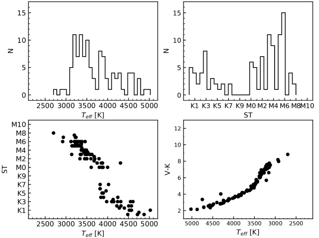
The photometric data of those stars are taken from literature as shown in Table 1. The T_eff and log $g$ of the sample giants (97 out of 107) are uniformly taken from McDonald et al. (2017), which are derived by comparing multi-wavelength archival photometry to BT-Settle model atmospheres. The uncertainties in their measurements are $\pm$ 125 K in T_eff. The parameters of the rest 10 giants are taken from other literature as mentioned in Table 1. The metallicity of only 32 giants in our sample are available in the literature (see, Table 1). Figure 1 represents T_eff and ST distribution of the sample, and their population in the T_eff $-$ ST and T_eff $-$ (V $-$ K) planes.

2.2 Data Reduction

The spectroscopic analysis is done using APALL task of IRAF. The TIRSPEC data have been reduced with TIRSPEC pipe-line¹¹1https://github.com/indiajoe/TIRSPEC/wiki (Ninan et al., 2014), and are cross-checked with the Image Reduction and Analysis Facility (IRAF ²²2http://iraf.noao.edu/). The data reduction consists of flat-fielding, sky subtraction, bad pixel correction, cosmic-ray removal, subtracting the pairs of images taken at two different slit positions, the wavelength calibration with Argon arc lamp, and finally, the spectrum extraction. To remove the telluric features of the Earth’s atmosphere the spectra of program stars are divided by the spectra of the standard star, which is taken on the same night. Prior to division, all hydrogen lines are removed from the spectra of the standard stars by interpolating the stellar continua. This is followed by the flux calibration of the target stars by using their Two Micron All Sky Survey (2MASS) H and K band photometric magnitudes.

3 Equivalent widths measurement

Table 3: Definitions of Spectral Bands to Measure Equivalent Widths.

Index	Feature	Feature	Continuum	Ref.
		Bandpass ( $\mu$ m)	Bandpass ( $\mu$ m)
SiI	Si I (1.59 $\mu$ m)	1.5870-1.5910	1.5830-1.5870, 1.5910-1.5950	1
CO1	¹²CO(2-0) (1.58 $\mu$ m)	1.5752-1.5812	1.5705-1.5745, 1.5830-1.5870	2
CO2	¹²CO(2-0) (1.62 $\mu$ m)	1.6175-1.6220	1.6145-1.6175, 1.6255-1.6285	1
NaI	Na I (2.21 $\mu$ m)	2.2040-2.2107	2.1910-2.1966, 2.2125-2.2170	3
CaI	Ca I (2.26 $\mu$ m)	2.2577-2.2692	2.2450-2.2560, 2.2700-2.2720	3
CO3	¹²CO(2-0) (2.29 $\mu$ m)	2.2910-2.3020	2.2420-2.2580, 2.2840-2.2910	2
CO4	¹²CO(3-1) (2.32 $\mu$ m)	2.3218-2.3272	2.2325-2.2345, 2.2695-2.2715	2

Ref : (1) Origlia et al. (1993); (2) This work; (3) Frogel et al. (2001)

The standard definition of equivalent width (EWs) is

EW_{\lambda}=\int_{\lambda 1}^{\lambda 2}\bigg{[}1-\frac{F(\lambda)}{F_{c}(\lambda)}\bigg{]}d\lambda

(1)

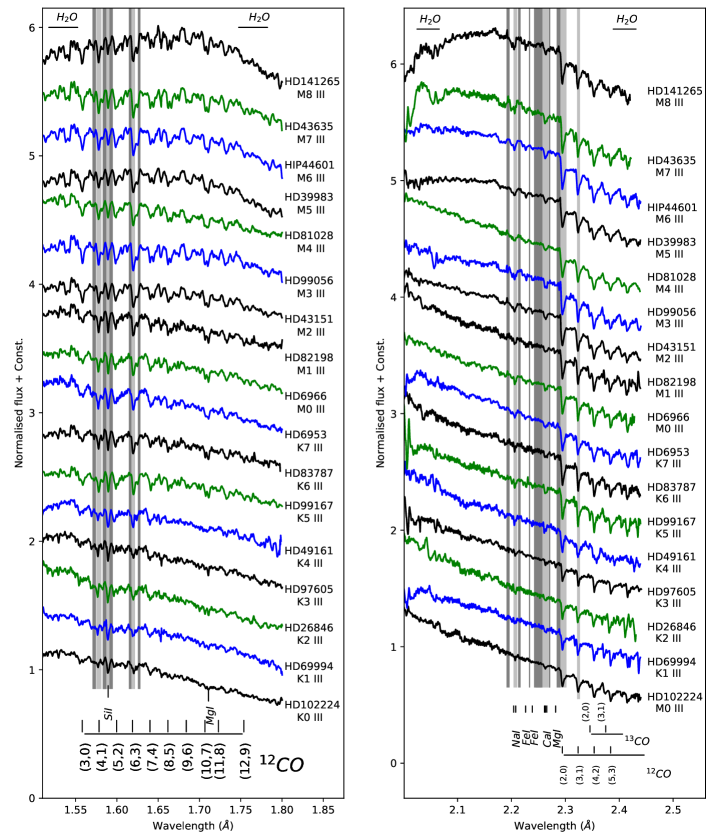
Here, F( $\lambda$ ) represents the flux density inside the feature bandpass from $\lambda 1$ to $\lambda 2$ , $F_{c}(\lambda)$ represents the value of the local continuum (Cesetti et al., 2013). To measure EWs feature band and continua bands are adopted as shown in Table 3 and in Figure 2. Bands of ¹²CO at 1.58 $\mu$ m are newly defined in this study. We compute the ¹²CO at 1.62 $\mu$ m band-strength according to the recipe of Origlia et al. (1993). Instead of four continua adopted by Frogel et al. (2001) to measure ¹²CO at 2.29 $\mu$ m absorption depth, we use here two continua as mentioned in Table 3. We adopt the feature bandpass of ¹²CO at 2.32 $\mu$ m from Kleinmann & Hall (1986), however, we use two different continua bands instead of one continuum used in Kleinmann & Hall (1986). Different continuum bands are also verified as mentioned in Ivanov et al. (2004); Cesetti et al. (2013), but better results are obtained from our selected band-passes.

Before computing EWs, the spectral features are corrected for the zero velocity by shifting. The EWs are estimated with the IDL script³³3https://github.com/ernewton/nirew (Newton et al., 2014). In the script, pseudo-continuum, i.e. continuum in featured bandpass, is defined by fitting a straight line through the continuum bandpass and EWs are measured by numerically integrating (trapezoidal method) the flux within the feature bandpass.

The average spectral resolution of TIRSPEC data is, R $\sim$ 1200. The spectral resolution varies with wavelengths and such resolution variation in TIRSPEC can be found in Ninan et al. (2014). The resolution of SpeX data is R $\sim$ 2000. The SpeX spectra are degraded to the same spectral resolution as of TIRSPEC before all the indices are estimated. Uncertainties on the EWs are computed with the Monte Carlo approach in the IDL script. The script adds normally-distributed (Gaussian) random noise to the stars’ spectrum by using RANDOMN function (Newton et al., 2014). Provided errors (photon, residual sky, and read noise) in SpeX pipeline are used for Gaussian random noise simulation to estimate uncertainties in EWs. But, our TIRSPEC pipeline does not provide such errors, and the errors are estimated using the technique provided by Stoehr et al. (2008). The computed EWs of our sample are listed in Table 5 along with their uncertainties.

4 RESULT AND DISCUSSION

4.1 Behaviour of spectral features

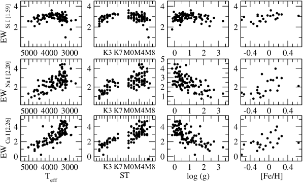
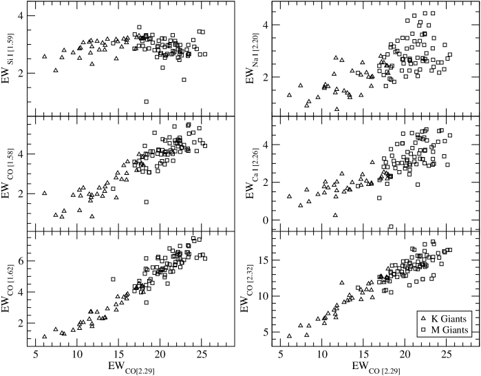
We have studied here the behaviour of spectral signatures of the giants with stellar atmospheric parameters like T_eff, ST, log $g$ and [Fe/H]. The most prominent atomic lines of HK band spectra are Si I at 1.59 $\mu$ m, Na I at 2.20 $\mu$ m, and Ca I at 2.26 $\mu$ m as shown in Figure 2. EWs of those lines are estimated using the methods as described in section 3. The behaviour of those lines with T_eff, ST, log $g$ , and [Fe/H] are shown in Figure 3. The Si I lines is one of the strongest absorption features in K giants, and it’s strength steadily increases as the temperature decreases from 5000 to 4000 K, after that remains unchanged up to 3500 K and decreases further below 3500 K. The corresponding behaviour of Si I with ST is also observed, e.g., increasing in the range K0 $-$ K7, unchanged to M4 and decreasing further, and it appears insensitive to the log $g$ .

The strengths of Na I and Ca I strongly depend on $T_{eff}$ and show an increasing trend with decreasing T_eff as found by others (Kleinmann & Hall, 1986; Ramírez et al., 1997; Förster Schreiber, 2000; Frogel et al., 2001; Ivanov et al., 2004; Rayner et al., 2009; Cesetti et al., 2013). Correlation of Na I line with ST shows increasing strength for K-giants, but no trend is conclusive for M giants. In the case of Ca I, the strength indicates an increasing trend with ST, similar to T_eff. The Na I and Ca I lines get stronger with decreasing log $g$ .

There is a significant dispersion in both correlations (T_eff and ST) for all the atomic lines. The poor band strengths in our medium-resolution spectra have some important role in such dispersion. Furthermore, contamination from other atomic lines are also affecting such studies, and relatively better spectral resolution are required for better characterization. Origlia et al. (1993) mentioned that Si I feature is somewhat contaminated by OH line at lower temperature and strength of OH line dominated beyond M2, i.e., T_eff $\leq$ 3800 K. The Na doublet at 2.2 $\mu$ m are blended with metallic lines like Si I (2.2069 $\mu$ m), Sc I (2.2058 and 2.2071 $\mu$ m) and V I (2.2097 $\mu$ m) in our medium-resolution spectra, and such dispersion in M-giants might be related to other lines behaviour (Wallace & Hinkle, 1996). For late M-giants, few low excitation lines like Ti I (2.2627 and 2.2639 $\mu$ m) and Sc I (2.2642 and 2.2663 $\mu$ m) contaminate the Ca triplet at 2.26 $\mu$ m.

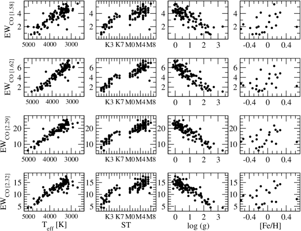
In the 1.5 $-$ 2.4 $\mu$ m regions, the first-overtone ( $\Delta\nu$ =2) and the second-overtone ( $\Delta\nu$ =3) band heads of ¹²CO are the dominant features in K $-$ M giants, and show increasing strength from K to M. In Figure 4, comparative behaviour of different CO bandheads (1.58 (CO1), 1.62 (CO2), 2.29 (CO3) and 2.32 (CO4) $\mu$ m) with T_eff, ST, log $g$ and [Fe/H] show an increasing trend of band strengths with decreasing T_eff, early to late ST, and decreasing value of log $g$ (see, e.g., Origlia et al. 1993; Ramírez et al. 1997; Cesetti et al. 2013). The behaviour of EWs with metallicity [Fe/H] in Figure 3 and Figure 4 does not show any conclusive trend as expected because most of our sample belong to solar-neighbourhood giants.

To investigate the origin of the dispersion especially in Figure 3, we plot index-index relations as shown in Figure 5. Figure 5 shows a tight index-index correlation at least for CO[1.62] $-$ CO[2.29] and CO[2.32] $-$ CO[2.29] as CO-bands are strong features in the medium-resolution spectra. Small dispersion of CO index-index correlations might be due to various reasons, such as the variation of abundance ratios, residuals of telluric lines. Note that we discard the known Mira variables and OH/IR stars belonging to M-spectral type of the IRTF library due to their large variability, and they might have different behaviour compared to the static giants (Lançon & Wood, 2000).

4.2 Empirical Calibrations

Table 4: Comparison between Goodness of Fit for various correlations.

Index	T	N	R	Rsqr	SEE	a0 $\dagger$	a1 $\dagger$	a2 $\dagger$	Remarks*
					T_eff	= f(EW) :
¹²CO (4-1)	107	101	0.90	0.82	207	5114 $\pm$ 70	-390 $\pm$ 19	-	1
1.58 $\mu$ m	98	93	0.90	0.82	197	5070 $\pm$ 69	-372 $\pm$ 19	-	2
(CO1)	70	67	0.90	0.82	177	5039 $\pm$ 68	-346 $\pm$ 20	-	3
¹²CO (6-3)	107	102	0.96	0.92	140	5049 $\pm$ 42	-279 $\pm$ 8	-	1
1.62 $\mu$ m	98	95	0.96	0.92	130	5038 $\pm$ 40	-274 $\pm$ 8	-	2
(CO2)	70	67	0.96	0.92	124	5092 $\pm$ 45	-287 $\pm$ 11	-	3
¹²CO (2-0)	107	100	0.96	0.93	130	5619 $\pm$ 54	-103 $\pm$ 3	-	1
2.29 $\mu$ m	98	93	0.97	0.93	119	5563 $\pm$ 51	-99 $\pm$ 3	-	2
(CO3)	70	67	0.97	0.94	104	5571 $\pm$ 53	-99 $\pm$ 3	-	3
¹²CO (3-1)	107	100	0.94	0.88	166	5603 $\pm$ 71	-149 $\pm$ 5	-	1
2.32 $\mu$ m	98	94	0.95	0.90	147	5549 $\pm$ 64	-143 $\pm$ 5	-	2
(CO4)	70	65	0.95	0.91	127	5532 $\pm$ 65	-140 $\pm$ 6	-	3
					log $g$	= f(EW) :
CO2	97	92	0.91	0.82	0.29	2.69 $\pm$ 0.01	-0.40 $\pm$ 0.02	-	1
CO3	97	93	0.93	0.86	0.29	3.75 $\pm$ 0.13	-0.16 $\pm$ 0.01	-	1
					T_eff	= f(EW, log $g$ ) :
CO2	97	90	0.99	0.97	78	4148 $\pm$ 72	-142 $\pm$ 11	315 $\pm$ 25	1
CO3	97	92	0.98	0.96	90	4465 $\pm$ 116	-54 $\pm$ 5	308 $\pm$ 30	1

T - total nos. of data points; N - no. of points used for fitting after eliminating 2 $\sigma$ outlayers
R - correlation coefficient; Rsqr - coefficient of determination; SEE - standard error of estimate
$\dagger$ T_eff = a0 + a1 $\times$ EWs + a2 $\times$ log $g$
*1 - Fitting with all the sample stars
*2 - Fitting with sample stars; T_eff $\geq$ 3200
*3 - Fitting with sample stars; T_eff $\geq$ 3400

4.2.1 Correlation between Effective Temperature and Equivalent Width

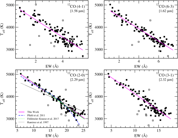
The most strong CO(2 $-$ 0) bandhead at 2.29 $\mu$ m has been widely used as a stellar $T_{eff}$ indicator. Several index definitions have been adopted to measure its strength (see Kleinmann & Hall 1986; Ramírez et al. 1997; Frogel et al. 2001; Blum et al. 2003; Maness et al. 2007; Mármol-Queraltó et al. 2008). Different index definitions lead to overestimation of the stellar temperatures (see Pfuhl et al. 2011). Pfuhl et al. (2011) computed the CO strength according to the recipe of Frogel et al. (2001) to determine T_eff using thirty-three giants with ST G0 $-$ M7, and have found smaller systematic error than other definitions. Other ¹²CO bandheads at 2.32 $\mu$ m and 1.62 $\mu$ m are also used as a reasonable good temperature indicator (see Kleinmann & Hall 1986; Origlia et al. 1993; Ivanov et al. 2004; Schultheis et al. 2016). Schultheis et al. (2016) showed ¹²CO(3 $-$ 1) bandhead at 2.32 $\mu$ m is an excellent temperature indicator in alternative of the strong ¹²CO bandhead at 2.29 $\mu$ m.

We used all of the four bandheads CO1, CO2, CO3, and CO4 for new empirical relations of the giants, and for relative comparison of their effectiveness. Following Origlia et al. (1993) and Frogel et al. (2001), we have used the bandpasses as mentioned in Table 3. In case of CO1, we have defined here new bandpasses as in Table 3 that has not explored earlier. For CO3 and CO4, we have used two bands of the continuum from Frogel et al. (2001), where the authors had used four bands of the continuum. The estimated EWs for all the sample stars are listed in Table 5. The EW of COs is plotted against T_eff shown in Figure 6. To establish the empirical relation between EW of COs and T_eff, a linear fit is explored for each bandhead separately using the linear equation T_eff = a0 + a1 $\times$ EWs (where, a0, a1 are the coefficients of the fit). The 2 $\sigma$ outliers are excluded for such fittings. Three different cases are excised for the best-fit, where case 1 is considered for all the 107 giants in our sample, case 2 for T_eff $\geq$ 3200 with 98 giants and case 3 for T_eff $\geq$ 3400 with 70 giants. The result of fitting in three different cases are listed in Table 4. The best-fit is judged by the three parameters $-$ correlation coefficient(R), the coefficient of determination (Rsqr) and the standard error of estimate (SEE). In case 1 (all the sample), SEE are 207 K, 140 K, 130 K, and 166 K for CO1, CO2, CO3, and CO4, respectively. In a comparison with all four bandheads, the SEE is minimum in case of strong bandhead CO3. We find that a better fit is obtained by narrowing down the temperature range and SEE improves from case 1 to case 3 for all bandheads. The least-square linear fits for case 1 only are shown in Figure 6. For comparison, the existing relations in the literature are also over-plotted in Figure 6, where the green dot line is the linear-fit from Feldmeier-Krause et al. (2017), blue dash line is the three-degree polynomial fit of the Pfuhl et al. (2011) and black dot-dashed line is the linear fit from Ramírez et al. (1997).

To establish the empirical relations, Feldmeier-Krause et al. (2017) used 69 stars with luminosity classes II-IV at a R $\sim$ 3310 $-$ 4660, Pfuhl et al. (2011) used 33 giants at R $\sim$ 2000 and R $\sim$ 3000, and Ramírez et al. (1997) used 43 giants at R $\sim$ 1380 and R $\sim$ 4830. Our correlation with T_eff $-$ CO3 differs significantly from the correlation of Ramírez et al. (1997), and the difference could be due to different bandpass and continuum used to measure EWs. However, the correlation of T_eff $-$ CO3 agrees well with that of Pfuhl et al. (2011) for T_eff > 3000 K and Feldmeier-Krause et al. (2017). However, we reproduced almost the same or better correlation with lower residual scatter (SEE) in spite of using the lower resolution spectra. It is important to note here that spectral resolution (i.e. R $\sim$ 3310 $-$ 4660 vs. R $\sim$ 1200) is insensitive to the T_eff $-$ CO3 correlation as seen in Feldmeier-Krause et al. (2017). Also, EWs of CO3 (2.29) are estimated using the two continuum bands, out of four continua as in Frogel et al. (2001). However, our established correlation shows no significant variation compared with the relations of Pfuhl et al. (2011) and Feldmeier-Krause et al. (2017) as shown in Figure 6, where the authors had used four continua of Frogel et al. (2001). Thus, two continua could be used instead of four to calculate EWs of CO3 without any systematic offset.

We also investigate simple parametrizations of the multi-line functions (e.g., CO1 $-$ SiI, CO1/SiI, CO2/CO1, CO2 $-$ CO1, CO3 $-$ (NaI+CaI), CO3/(NaI+CaI), etc.), and perform least-square regression to test the correlation with T_eff for each combination qualitatively. No combining feature results significant improvement of the relationship discussed above. It is noted that the correlation between combined features follows the trends of the stronger feature of that combination. Further discussion on the combined features is therefore excluded.

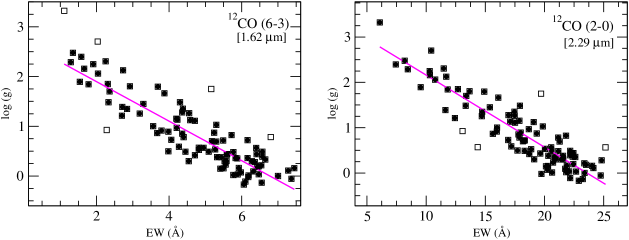
4.2.2 Correlation between Surface Gravity and Equivalent Width

To establish the empirical relation between EWs and log $g$ , a linear fit is explored for CO2 and CO3 bandhead separately using the linear equation log $g$ = $a_{0}$ + $a_{1}$ $\times$ EWs. We have used here CO2 and CO3 bands as their SNR are relatively better than other CO bands. Among 107 giants, 97 have known log $g$ in the literature and we have used here for the fit. We excluded the limiting 2 $\sigma$ outliers for fitting. The least-square linear fits are shown in Figure 7. The number of the stars used for the fit after 2 $\sigma$ clipping and the coefficients of fit are listed in Table 4 along with SEE. The best-fit is judged on the basis of SEE, which is 0.29 for both bands. Our study suggests that both CO2 and CO3 are good log $g$ indicator and the result differs from Origlia et al. (1993), who demonstrated that CO2 is a better representative of log $g$ than CO3 from the behaviour of synthetic spectra.

4.2.3 Effect of Surface Gravity on Effective Temperature vs Equivalent Width correlation

To take into account the effects of log $g$ on the calibration of T_eff and the EWs of ¹²CO at 1.62 and 2.29 $\mu$ m, we recalibrate the empirical relations as,

T_{eff}=a_{0}+a_{1}{EW}+a_{2}\log{g}.

(2)

where, $a_{i}$ (i=0,…,2) are the coefficients of the fit obtained iteratively. The SEE corresponds to 78 and 90 K for CO2 and CO3, respectively. The results of fitting are listed in Table 4. To test the effects of log $g$ quantitatively, we fit the equation (2) without considering log $g$ i.e. making $a_{2}$ =0. The SEE is equivalent to 132 K for both cases. It is noted that the SEE is improved significantly when the effect of log $g$ is considered in the T_eff vs EWs correlation. However, we did not consider the metallicity effect on T_eff $-$ CO correlation since metallicity is unavailable for most of the stars in our sample. Schultheis et al. (2016) found no critical metallicity dependence on the T_eff $-$ CO[2.29] correlation in the temperature range 3200 $-$ 4500 K within metallicity range $-$ 1.2 to +0.5 dex.

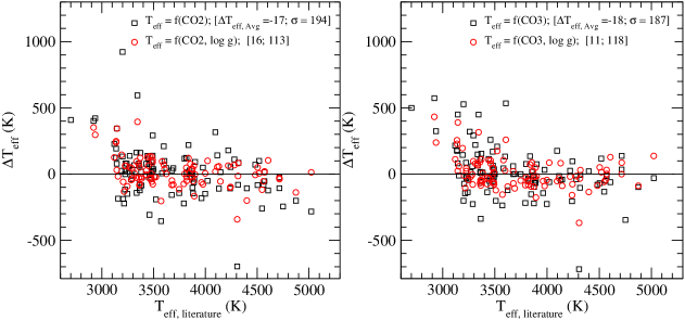
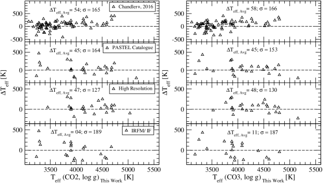
The T_eff obtained from our empirical calibrations are compared with the previous published values of T_eff estimated using various techniques. It is to be noted that we obtain the best T_eff considering the effect of log $g$ along with the EWs of CO as described earlier. Hence, we derive values of T_eff from the equation 2 using both CO2 and CO3 features, and compare distinctly with the literature values as shown in Figure 9. First, we focus on the Catalog of Earth-Like Exoplanet Survey Targets (CELESTA), a database of habitable zones around 37000 nearby stars (Chandler, McDonald & Kane, 2016). We have 85 giants in common with our current sample of giants, but 5 of them (HD92620, HD115322, HD7861, HIP44601, HD141265) have not been considered owing to absence of log $g$ values in the literatures. We find that their T_eff are on average $\sim$ 50 K cooler than our measurements, with a standard deviation, $\sigma$ $\sim$ 165 K for both (CO2 and CO3) cases. A total of 27 giants are found in common with PASTEL catalogue (Soubiran et al., 2016). We find that the T_eff of giants obtained in this work are on average 45 K warmer than the measurement in the PASTEL catalogue, with $\sigma$ $\sim$ 155 K. Estimation of T_eff from high resolution spectra are available for 25 giants with our current sample⁴⁴4HD54810, HD137759 (Jofré et al., 2015); HD99283 (Reffert et al., 2015); HD102224, HD70272, HD60522, HD124897 (Hekker & Meléndez, 2007); HD69994, HD26846, HD97605, HD83787, HD91810, HD178208 (Feuillet et al., 2016); HD85503 (Bruntt, Frandsen & Thygesen, 2011); HD30834, HD92523, HD49161, HD99167, HD35620, HD99998, HD120477 (McWilliam, 1990); HD100006 (Luck & Heiter, 2007); HD25975, HD19058 Smith & Lambert (1986); HD207991 Kovtyukh (2007).. A comparison of common objects provide an average difference of 16 K (CO2) and 11 K (CO3), with $\sigma$ = 113 K (CO2) and 118 K (CO3). T_eff of 4 giants are derived from IRFM method⁵⁵5HD54810 (Blackwell & Lynas-Gray, 1998); HD219215, HD35620, HD99998 (Alonso, Arribas & Martínez-Roger, 1999a) and 16 giants are measured from interferometric data⁶⁶6HD102224, HD85503, HD92523, HD70272, HD99167, HD6953, HD38944, HD60522, HD216397, HD137759, HD120477, HD3346 (Bordé, Coudé, Chagnon & Perrin, 2002), HD18191, HD175865, HD196610, HD108849 (Dyck & van Belle, 1998). The mean difference is $\sim$ 10 K, with $\sigma$ $\sim$ 180 K considering all the 20 giants.

4.3 Application of our empirical relations

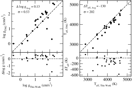
To inspect reliability of our empirical relations, we estimate T_eff and log $g$ from the spectra (R $\sim$ 1250) of K $-$ M giants observed with Near Infrared Camera Spectrometer (NICS) on 3.58 m Telescopic Nazionale Galileo (TNG) at Roque de los Muchachos Observatory, La Palma, Spain (Mármol-Queraltó et al., 2008). A total of 25 K $-$ M giants yield the opportunity to compare the parameters measured from our empirical relations with that of literature values⁷⁷7https://webs.ucm.es/info/Astrof/ellipt/CO.html. The log $g$ is estimated from log $g$ $-$ CO3 relation. The results are in good agreement with average difference, $\Delta\log g_{Avg}$ = 0.13 $cm/s^{2}$ and standard deviation, $\sigma$ = 0.53 $cm/s^{2}$ . The T_eff are estimated using the measured log $g$ and CO3 from equation 2. The T_eff are on average 130 K cooler than literature value with a standard deviation, $\sigma$ = 202 K. Excluding the two giants, HD232708 (residual=572 K), a long period variable and HD126327 (residual=448 K), an asymptotic giant branch star, the $\Delta T_{eff,Avg}$ and $\sigma$ reduce to -97 K and 146 K respectively. The origin of this discrepancies might be due to the fact that pulsating long period variables behave differently than the static giants (Bessell et al., 1989; Alvarez & Plez, 1998; Lançon & Wood, 2000; Ghosh et al., 2018). The dispersion of two fundamental parameters from our measurements is shown in Figure 10.

5 Summary and Conclusions

We have constructed a new medium resolution (R $\sim$ 1200) NIR (1.50 $-$ 2.45 $\mu$ m) spectral library of 72 K $-$ M giant stars with the aim of populating existing NIR stellar libraries with cool giants specifically after the M3 spectral type. The EWs of prominent atomic (Si I at 1.59 $\mu$ m, Na I at 2.20 $\mu$ m, Ca I at 2.26 $\mu$ m) and molecular (¹²CO first overtone bandheads at 2.29 $\mu$ m, 2.32 $\mu$ m and, second overtone bandheads at 1.58 $\mu$ m, 1.62 $\mu$ m) are estimated. We have studied here the behaviour of those EWs with the fundamental parameters (e.g., effective temperature, spectral type, surface gravity, and metallicity). The main results are summarized as

1.

We obtained reliable new empirical relations between the EWs of ¹²CO bandheads and T_eff. We found that the ¹²CO first overtone band at 2.29 $\mu$ m and second overtone band at 1.62 $\mu$ m are reasonably good temperature indicator above 3400 K. This relation is also insensitive to the spectral resolution, and therefore, could be used more generally.
2.

We present the empirical calibrations between the EWs of ¹²CO bandheads (CO2 and CO3) and log $g$ . Our study suggests that both ¹²CO are a very good indicator of log $g$ .
3.

We find that the significant improvement of empirical relations between ¹²CO and T_eff on the inclusion of log $g$ , and more reliable T_eff could be predicted. However, we do not investigate the metallicity effects of these correlations from such medium-resolution spectra in narrow metallicity range of our sample. Further investigation regarding metallicity from high-resolution spectra would be greatly appreciated.

Acknowledgements

The authors are very much thankful to the reviewer, Dr. R. Peletier, for his critical and valuable comments, which helped us to improve the paper. This research work is supported by S N Bose National Centre for Basic Sciences under Department of Science and Technology, Government of India. The authors thank the staff of IAO, Hanle and CREST, Hosakote, who made these observations possible. The facilities at IAO and CREST are operated by the Indian Institute of Astrophysics, Bangalore. We acknowledge the usage of the TIFR Near Infrared Spectrometer and Imager (TIRSPEC). SG is thankful to Joe Philip Ninan for helpful discussions and valuable suggestions about the data reduction on TIRSPEC-pipeline.

References

Alonso, Arribas & Martínez-Roger (1999a) Alonso, A., Arribas, S., Martínez-Roger, C., 1999, A&AS, 139, 335
Alvarez & Plez (1998) Alvarez, R., Plez, B., 1998, A& A, 330, 1109
Bessell et al. (1989) Bessell, M. S., Brett, J. M., Wood, P. R., Scholz, M., 1989, A&A, 213, 209
Blackwell & Lynas-Gray (1998) Blackwell, D. E., Lynas-Gray, A. E., 1998, A&AS, 129, 505
Blum et al. (1996) Blum, R. D., Sellgren, K., Depoy, D. L., 1996, AJ, 112, 1988
Blum et al. (2003) Blum, R. D., Ramírez, Solange V., Sellgren, K., Olsen, K., 2003, ApJ, 597, 323
Boeche, Smith & Grebel et al. (2018) Boeche, C., Smith, M. C., Grebel, E. K., et al., 2018, AJ, 155, 181
Bordé, Coudé, Chagnon & Perrin (2002) Bordé, P., Coudé du Foresto, V., Chagnon, G., Perrin, G., 2002, A&A, 393, 183
Bruntt, Frandsen & Thygesen (2011) Bruntt, H., Frandsen, S., Thygesen, A. O., 2011, A&A, 528, 121
Cenarro et al. (2001) Cenarro, A. J., Gorgas, J., Cardiel, N., et al. 2001, MNRAS, 326, 981
Cenarro et al. (2007) Cenarro, A. J., Peletier, R. F., Sánchez-Blázquez, P., et al. 2007, MNRAS, 374, 664
Cesetti et al. (2013) Cesetti, M., Pizzella, A., Ivanov, V. D., Morelli, L., Corsini, E. M., Dalla Bontà, E., 2013, A&A, 549, 129
Chandler, McDonald & Kane (2016) Chandler, C. O., McDonald, I., Kane, S. R., 2016, AJ, 151, 59
Chen et al. (2014) Chen, Yan-Ping, Trager, S. C., Peletier, R. F., Lançon, A., Vazdekis, A., Prugniel, Ph., Silva, D. R., Gonneau, A., 2014, A& A, 565, 117
Cushing et al. (2005) Cushing, Michael C., Rayner, John T., Vacca, William D., 2005, ApJ, 623, 1115
Dyck & van Belle (1998) Dyck, H. M.; van Belle, G. T.; Thompson, R. R., 1998, AJ, 116, 981
Eisenstein et al. (2011) Eisenstein, D. J., Weinberg, D. H., Agol, E., et al. 2011, AJ, 142, 72
Feldmeier-Krause et al. (2017) Feldmeier-Krause, A., Kerzendorf, W., Neumayer, N. et al., 2017, MNRAS, 464, 194
Feuillet et al. (2016) Feuillet, D. K.; Bovy, Jo; Holtzman, J., et al, 2016, ApJ, 817, 40
Figer et al. (1995) Figer, D. F., McLean, I. S., & Morris, M. 1995, ApJ, 447, L29
Förster Schreiber (2000) Förster Schreiber, N. M., 2000, AJ, 120, 2089
Frogel et al. (2001) Frogel, Jay A., Stephens, Andrew, Ramírez, Solange, DePoy, Darren L., 2001, AJ, 122, 1896
Garrison (1994) Garrison, R. F. 1994, in ASP Conf. Ser. 60, The MK Process at 50 Years: A Powerful Tool for Astrophysical Insight, ed. C. J. Corbally, R. O. Gray, & R. F. Garrison (San Francisco, CA: ASP), 3
Gáspár, Rieke & Ballering (2016) Gáspár, A., Rieke, George H., Ballering, N., 2016, ApJ, 826, 171
Gautschy-Loidl et al. (2004) Gautschy-Loidl, R., Höfner, S., Jørgensen, U. G., & Horn, J. 2004, A&A, 422, 289
Ghosh et al. (2018) Ghosh, Supriyo; Mondal, Soumen; Das, Ramkrishna, et al. 2018, AJ, 155, 216
Greene & Meyer (1995) Greene, T. P., & Meyer, M. R. 1995, ApJ, 450, 233
Hekker & Meléndez (2007) Hekker, S.; Meléndez, J., 2007, A&A, 475, 1003
Ho et al. (2017) Ho, A. Y. Q., Ness, M. K., Hogg, D. W., et al. 2017, ApJ, 836, 5
Ivanov et al. (2004) Ivanov, V. D., Rieke, M. J., Engelbracht, C. W., Alonso-Herrero, A., Rieke, G. H., Luhman, K. L., 2004, ApJS, 151, 387
Johnson & Méndez (1970) Johnson, H. L., Méndez, M. E., 1970, AJ, 75, 785
Jofré et al. (2015) Jofré, E., Petrucci, R., Saffe, C., et al., 2015, A&A, 574, 50
Joyce et al. (1998) Joyce, Richard R., Hinkle, Kenneth H., Wallace, Lloyd, Dulick, Michael, Lambert, David L., 1998, AJ, 116, 2520
Kleinmann & Hall (1986) Kleinmann, S. G., Hall, D. N. B., 1986, ApJS, 62, 501
Kovtyukh (2007) Kovtyukh, V. V., 2007, MNRAS, 378, 617
Kurtev et al. (2007) Kurtev, R., Borissova, J., Georgiev, L., Ortolani, S., & Ivanov, V. D. 2007, A&A, 475, 209
Lançon & Wood (2000) Lançon, A., Wood, P. R., 2000, A&AS, 146, 217
Lançon et al. (2007) Lançon, A., Hauschildt, P. H., Ladjal, D., Mouhcine, M., 2007, A& A, 468, 205
Le Borgne et al. (2003) Le Borgne, J.-F., Bruzual, G., Pelló, R., et al. 2003, A&A, 402, 433
Liu et al. (2014) Liu X.-W. et al., 2014, in Feltzing S., Zhao G., Walton N., Whitelock P., eds, Proc. IAU Symp. 298, Setting the Scene for Gaia and LAMOST. Cambridge Univ. Press, Cambridge, p. 310 LSST Science Collaboration, 2009, preprint (arXiv:0912.0201)
Luck & Heiter (2007) Luck, R. E., Heiter, U., 2007, AJ, 133, 2464
Luo et al. (2016) Luo, A.-L., Zhao, Y.-H., Zhao, G., et al. 2016, yCat, 5149, 0
Maness et al. (2007) Maness, H., Martins, F., Trippe, S. et al., 2007, ApJ, 669, 1024
Massarotti et al. (2008) Massarotti, A., Latham, D. W., Stefanik, R. P., Fogel, J., 2008, AJ, 135, 209
Mármol-Queraltó et al. (2008) Mármol-Queraltó, E., Cardiel, N., Cenarro, A. J., Vazdekis, A., Gorgas, J., Pedraz, S., Peletier, R. F., Sánchez-Blázquez, P., 2008, A&A, 489, 885
McDonald et al. (2012) McDonald, I., Zijlstra, A. A., Boyer, M. L., 2012, MNRAS, 427, 343
McDonald et al. (2017) McDonald, I., Zijlstra, A. A., Watson, R. A., 2017, MNRAS, 471, 770
McWilliam (1990) McWilliam, A., 1990, ApJS, 74, 1075
Meyer et al. (1998) Meyer, Michael R., Edwards, Suzan, Hinkle, Kenneth H., Strom, Stephen E., 1998, ApJ, 508, 397
Morgan et al. (1943) Morgan, W. W., Keenan, P. C., & Kellman, E. 1943, An Atlas of Stellar Spectra, with an Outline of Spectral Classification (Chicago, IL: Univ. Chicago Press)
Newton et al. (2014) Newton, Elisabeth R., Charbonneau, David, Irwin, Jonathan, Berta-Thompson, Zachory K., Rojas-Ayala, Barbara, Covey, Kevin, Lloyd, James P., 2014, AJ, 147, 20
Ninan et al. (2014) Ninan, J. P., Ojha, D. K., Ghosh, S. K., et al. 2014, JAI, 3, 1450006
Origlia et al. (1993) Origlia, L., Moorwood, A. F. M., Oliva, E., 1993, A&A, 280, 536
Perryman et al. (2001) Perryman M. A. C. et al., 2001, A&A, 369, 339
Peterson et al. (2008) Peterson, D. E., et al. 2008, ApJ, 685, 313
Pfuhl et al. (2011) Pfuhl, O., Fritz, T. K., Zilka, M., Maness, H., Eisenhauer, F., Genzel, R., Gillessen, S., Ott, T., Dodds-Eden, K., Sternberg, A., 2011, ApJ, 741, 108
Prugniel & Soubiran (2001) Prugniel, P., & Soubiran, C. 2001, A& A, 369, 1048
Prugniel et al. (2011) Prugniel, P., Vauglin, I., & Koleva, M. 2011, A&A, 531, A165
Ramírez & Meléndez (2005) Ramírez I., Meléndez J., 2005, ApJ, 626, 465
Ramírez et al. (1997) Ramírez, S. V., Depoy, D. L., Frogel, Jay A., Sellgren, K., Blum, R. D., 1997, AJ, 113, 1411
Rayner et al. (2009) Rayner, J. T., Cushing, M. C., Vacca, W. D., 2009, ApJS, 185, 289
Reffert et al. (2015) Reffert, S., Bergmann, C., Quirrenbach, A., et al, 2015, A&A, 574, 116
Riffel et al. (2008) Riffel, R., Pastoriza, M. G.., Rodríguez-Ardila, A., & Maraston, C. 2008, MNRAS, 388, 803
Sánchez-Blázquez et al. (2006) Sánchez-Blázquez, P., Peletier, R. F., Jiménez-Vicente, J., et al. 2006, MNRAS, 371, 703
Schultheis et al. (2016) Schultheis, M., Ryde, N., Nandakumar, G., 2016, A& A, 590, 6
Smith & Lambert (1986) Smith, Verne V., Lambert, David L., 1986, ApJ, 311, 843
Soubiran et al. (2016) Soubiran, C., Le Campion, Jean-François, Brouillet, N., Chemin, L., 2016, A&A, 591, 118
Steinmetz et al. (2006) Steinmetz, M., Zwitter, T., Siebert, A., et al. 2006, AJ, 132, 1645
Stoehr et al. (2008) Stoehr, F., White, R., Smith, M., et al. 2008, ASPC, 394, 505
Terndrup et al. (1990) Terndrup, D. M., Frogel, Jay A., Whitford, A. E., 1990, ApJ, 357, 453
Valdes et al. (2004) Valdes, F., Gupta, R., Rose, J. A., Singh, H. P., & Bell, D. J. 2004, ApJS, 152, 251
van Belle et al. (1999) van Belle, G. T., Lane, B. F., Thompson, R. R., et al., 1999, AJ, 117, 521
Villaume et al. (2017) Villaume, A., Conroy, C., Johnson, B., Rayner, J., Mann, Andrew W., van Dokkum, P., 2017, ApJS, 230, 23
Wallace & Hinkle (1996) Wallace, L., Hinkle, K., 1996, ApJS, 107, 312
Wallace & Hinkle (1997) Wallace, L., Hinkle, K., 1997, ApJS, 111, 445
Wallace & Hinkle (2002) Wallace, Lloyd, Hinkle, Kenneth, 2002, AJ, 124, 3393
Wright et al. (2003) Wright, C. O., Egan, M. P., Kraemer, K. E., Price, S. D., 2003, AJ, 125, 359
Wu et al. (2011) Wu, Y., Singh, H. P., Prugniel, P., Gupta, R., Koleva, M., 2011, A&A, 525, 71
Yanny et al. (2009) Yanny, B., Newberg, H. J., Johnson, J. A., et al. 2009, ApJ, 700, 1282
Yuan et al. (2015) Yuan H.-B. et al., 2015, MNRAS, 448, 855

Appendix A Some extra material

Table 5: Measured Equivalent Widths of all the sample

Star Names	Si I	CO1	CO2	Na I	Ca I	CO3	CO4
			TIRSPEC :
HD54810	2.09 $\pm$ 0.24	0.91 $\pm$ 0.66	1.58 $\pm$ 0.23	1.67 $\pm$ 0.36	0.76 $\pm$ 0.44	7.44 $\pm$ 2.24	5.87 $\pm$ 1.13
HD99283	2.54 $\pm$ 0.56	0.82 $\pm$ 0.61	1.35 $\pm$ 0.29	0.90 $\pm$ 0.33	1.60 $\pm$ 0.64	8.19 $\pm$ 1.77	4.54 $\pm$ 1.88
HD102224	2.31 $\pm$ 0.86	0.84 $\pm$ 0.38	1.78 $\pm$ 0.46	0.76 $\pm$ 0.38	2.02 $\pm$ 0.34	11.82 $\pm$ 1.20	8.68 $\pm$ 0.92
HD69994	2.52 $\pm$ 1.14	1.15 $\pm$ 0.92	1.66 $\pm$ 0.66	1.57 $\pm$ 0.55	1.44 $\pm$ 0.53	10.32 $\pm$ 2.31	6.19 $\pm$ 1.53
HD40657	2.70 $\pm$ 0.28	1.64 $\pm$ 0.53	2.71 $\pm$ 0.34	1.40 $\pm$ 0.32	0.24 $\pm$ 0.76	11.63 $\pm$ 2.16	7.48 $\pm$ 2.27
HD85503	3.08 $\pm$ 0.47	1.97 $\pm$ 0.65	2.25 $\pm$ 0.60	2.11 $\pm$ 1.38	1.85 $\pm$ 1.16	11.49 $\pm$ 2.74	8.05 $\pm$ 1.91
HD26846	3.13 $\pm$ 0.60	1.81 $\pm$ 0.86	2.73 $\pm$ 0.48	2.73 $\pm$ 0.98	1.23 $\pm$ 0.71	11.70 $\pm$ 2.62	7.00 $\pm$ 2.15
HD30834	3.05 $\pm$ 0.38	1.87 $\pm$ 0.77	2.28 $\pm$ 0.35	1.39 $\pm$ 0.41	1.68 $\pm$ 0.51	13.08 $\pm$ 0.95	9.37 $\pm$ 1.71
HD92523	2.50 $\pm$ 0.46	1.79 $\pm$ 0.37	2.84 $\pm$ 0.31	1.30 $\pm$ 0.20	1.85 $\pm$ 0.34	14.74 $\pm$ 1.23	9.52 $\pm$ 1.27
HD97605	2.88 $\pm$ 0.92	1.89 $\pm$ 1.86	2.03 $\pm$ 0.73	1.71 $\pm$ 0.38	2.02 $\pm$ 0.70	10.43 $\pm$ 1.36	6.98 $\pm$ 1.71
HD49161	3.11 $\pm$ 0.24	1.97 $\pm$ 1.19	2.70 $\pm$ 0.56	2.64 $\pm$ 0.54	2.45 $\pm$ 0.90	12.43 $\pm$ 2.34	11.82 $\pm$ 1.59
HD70272	3.06 $\pm$ 0.49	2.69 $\pm$ 0.28	3.79 $\pm$ 0.62	1.65 $\pm$ 0.32	1.90 $\pm$ 0.40	15.97 $\pm$ 1.75	10.82 $\pm$ 1.32
HD99167	2.85 $\pm$ 0.27	3.56 $\pm$ 0.46	4.23 $\pm$ 0.65	2.80 $\pm$ 0.42	2.19 $\pm$ 0.78	17.11 $\pm$ 2.65	12.73 $\pm$ 2.78
HD83787	3.21 $\pm$ 0.67	3.45 $\pm$ 0.60	3.98 $\pm$ 1.15	2.14 $\pm$ 0.71	2.41 $\pm$ 0.51	17.99 $\pm$ 1.97	13.78 $\pm$ 2.12
HD6953	3.22 $\pm$ 0.33	3.61 $\pm$ 0.53	3.87 $\pm$ 0.41	2.02 $\pm$ 0.28	3.05 $\pm$ 0.53	16.10 $\pm$ 1.50	9.79 $\pm$ 1.65
HD6966	2.95 $\pm$ 0.77	3.11 $\pm$ 0.44	4.30 $\pm$ 0.96	2.87 $\pm$ 0.36	2.81 $\pm$ 0.45	17.93 $\pm$ 1.73	12.23 $\pm$ 2.18
HD18760	3.04 $\pm$ 0.84	2.25 $\pm$ 0.64	4.82 $\pm$ 0.61	2.16 $\pm$ 0.52	1.80 $\pm$ 0.84	14.36 $\pm$ 1.67	11.17 $\pm$ 3.13
HD38944	2.85 $\pm$ 0.76	3.61 $\pm$ 1.10	4.06 $\pm$ 0.31	2.43 $\pm$ 0.55	1.17 $\pm$ 1.02	16.93 $\pm$ 2.42	11.93 $\pm$ 1.10
HD60522	3.60 $\pm$ 0.80	3.66 $\pm$ 0.60	4.71 $\pm$ 1.30	2.76 $\pm$ 0.20	3.26 $\pm$ 0.26	17.51 $\pm$ 1.58	10.72 $\pm$ 1.36
HD216397	2.95 $\pm$ 0.58	3.22 $\pm$ 1.11	4.38 $\pm$ 0.87	2.08 $\pm$ 0.41	2.82 $\pm$ 0.71	17.46 $\pm$ 1.88	12.26 $\pm$ 1.81
HD7158	2.83 $\pm$ 1.09	4.41 $\pm$ 0.49	5.18 $\pm$ 0.41	1.94 $\pm$ 0.40	2.34 $\pm$ 0.46	18.18 $\pm$ 0.68	12.06 $\pm$ 2.28
HD82198	3.12 $\pm$ 0.83	3.88 $\pm$ 0.46	4.20 $\pm$ 0.40	2.20 $\pm$ 0.46	1.92 $\pm$ 0.33	17.88 $\pm$ 2.15	12.50 $\pm$ 1.83
HD218329	3.33 $\pm$ 0.90	3.92 $\pm$ 0.65	4.58 $\pm$ 0.46	3.00 $\pm$ 0.99	4.03 $\pm$ 0.71	19.09 $\pm$ 4.36	12.66 $\pm$ 3.53
HD219215	2.91 $\pm$ 0.49	4.02 $\pm$ 0.64	5.16 $\pm$ 0.46	2.68 $\pm$ 0.70	4.06 $\pm$ 0.89	19.71 $\pm$ 1.73	13.02 $\pm$ 2.31
HD119149	3.29 $\pm$ 0.62	4.01 $\pm$ 0.60	5.49 $\pm$ 0.77	3.14 $\pm$ 0.47	2.29 $\pm$ 1.20	18.29 $\pm$ 3.03	13.40 $\pm$ 3.19
HD1013	3.13 $\pm$ 1.43	4.18 $\pm$ 1.20	5.30 $\pm$ 1.00	2.52 $\pm$ 0.96	3.34 $\pm$ 0.96	19.86 $\pm$ 2.58	12.79 $\pm$ 2.36
HD33463	2.97 $\pm$ 1.57	3.97 $\pm$ 1.46	4.54 $\pm$ 1.09	3.66 $\pm$ 0.77	3.82 $\pm$ 1.60	20.92 $\pm$ 2.07	16.58 $\pm$ 2.52
HD39732	2.77 $\pm$ 0.69	4.31 $\pm$ 0.71	5.32 $\pm$ 0.32	2.04 $\pm$ 0.39	1.88 $\pm$ 0.54	21.57 $\pm$ 2.52	13.75 $\pm$ 1.86
HD43151	2.62 $\pm$ 0.18	4.12 $\pm$ 0.41	5.56 $\pm$ 0.78	2.51 $\pm$ 0.26	3.51 $\pm$ 0.38	20.73 $\pm$ 1.24	14.10 $\pm$ 1.80
HD92620	2.91 $\pm$ 0.40	4.09 $\pm$ 0.24	5.42 $\pm$ 0.31	2.66 $\pm$ 0.23	2.99 $\pm$ 0.29	20.58 $\pm$ 1.26	14.50 $\pm$ 2.14
HD115521	3.19 $\pm$ 0.51	3.08 $\pm$ 0.66	4.71 $\pm$ 0.57	1.82 $\pm$ 0.25	2.96 $\pm$ 0.47	18.72 $\pm$ 1.77	13.01 $\pm$ 1.30
HD16058	2.83 $\pm$ 0.88	4.72 $\pm$ 0.51	6.57 $\pm$ 1.05	2.72 $\pm$ 0.63	3.23 $\pm$ 0.92	22.17 $\pm$ 2.81	12.35 $\pm$ 1.72
HD28168	3.21 $\pm$ 1.00	3.45 $\pm$ 1.61	3.98 $\pm$ 0.74	1.66 $\pm$ 1.01	3.06 $\pm$ 1.36	17.72 $\pm$ 10.61	10.83 $\pm$ 2.02
HD66875	2.75 $\pm$ 0.31	4.11 $\pm$ 0.73	5.60 $\pm$ 0.52	2.69 $\pm$ 0.40	3.72 $\pm$ 0.80	22.45 $\pm$ 1.23	14.07 $\pm$ 2.88
HD99056	2.46 $\pm$ 0.50	4.65 $\pm$ 0.67	6.41 $\pm$ 0.45	3.23 $\pm$ 0.44	4.38 $\pm$ 1.09	22.34 $\pm$ 2.38	15.08 $\pm$ 3.13
HD215953	3.12 $\pm$ 0.47	4.68 $\pm$ 1.53	5.72 $\pm$ 0.87	3.38 $\pm$ 1.26	4.34 $\pm$ 0.98	21.82 $\pm$ 2.74	14.04 $\pm$ 1.99
HD223637	3.20 $\pm$ 0.52	3.48 $\pm$ 0.73	4.95 $\pm$ 0.34	2.25 $\pm$ 0.76	2.42 $\pm$ 0.82	20.57 $\pm$ 2.78	11.50 $\pm$ 2.15
HD25921	3.26 $\pm$ 0.75	3.80 $\pm$ 0.98	6.16 $\pm$ 1.28	3.25 $\pm$ 0.49	3.76 $\pm$ 0.63	18.34 $\pm$ 2.13	12.78 $\pm$ 2.14
HD33861	3.43 $\pm$ 0.90	4.54 $\pm$ 1.14	6.40 $\pm$ 0.50	2.71 $\pm$ 0.41	2.93 $\pm$ 0.36	25.16 $\pm$ 1.58	16.41 $\pm$ 2.10
HD224062	2.66 $\pm$ 0.17	4.09 $\pm$ 0.66	5.53 $\pm$ 0.51	2.20 $\pm$ 0.61	2.96 $\pm$ 0.97	21.41 $\pm$ 1.86	12.01 $\pm$ 2.33
HD5316	3.13 $\pm$ 0.40	4.18 $\pm$ 0.44	5.30 $\pm$ 1.27	2.53 $\pm$ 0.61	4.10 $\pm$ 1.00	21.28 $\pm$ 1.51	13.79 $\pm$ 2.55
HD34269	2.62 $\pm$ 1.13	4.33 $\pm$ 0.58	5.88 $\pm$ 0.70	2.91 $\pm$ 0.59	4.81 $\pm$ 1.35	22.61 $\pm$ 3.61	14.24 $\pm$ 1.91
HD64052	2.99 $\pm$ 1.49	4.84 $\pm$ 1.17	6.80 $\pm$ 0.69	4.35 $\pm$ 0.66	3.10 $\pm$ 1.49	21.16 $\pm$ 3.74	16.43 $\pm$ 3.21
HD81028	2.70 $\pm$ 0.48	3.98 $\pm$ 0.51	5.41 $\pm$ 0.27	2.02 $\pm$ 0.24	2.88 $\pm$ 0.42	20.13 $\pm$ 1.39	12.84 $\pm$ 2.13
HD206632	2.98 $\pm$ 0.91	4.53 $\pm$ 0.59	6.47 $\pm$ 0.60	4.44 $\pm$ 0.73	4.72 $\pm$ 1.64	22.44 $\pm$ 3.05	14.41 $\pm$ 3.79
HD16896	2.67 $\pm$ 0.46	3.68 $\pm$ 0.75	5.83 $\pm$ 1.08	3.14 $\pm$ 0.63	4.61 $\pm$ 1.33	20.86 $\pm$ 2.45	15.38 $\pm$ 2.37
HD17491	3.21 $\pm$ 1.36	3.64 $\pm$ 0.72	5.98 $\pm$ 0.72	3.09 $\pm$ 0.55	3.14 $\pm$ 0.44	20.25 $\pm$ 2.52	14.86 $\pm$ 2.12
HD17895	2.95 $\pm$ 1.33	3.14 $\pm$ 0.79	6.18 $\pm$ 0.50	3.50 $\pm$ 0.53	4.07 $\pm$ 0.47	19.74 $\pm$ 1.48	14.21 $\pm$ 1.95
HD22689	2.82 $\pm$ 0.41	4.21 $\pm$ 0.77	6.55 $\pm$ 0.86	2.25 $\pm$ 0.85	3.87 $\pm$ 0.57	23.24 $\pm$ 3.49	12.41 $\pm$ 2.22
HD26234	2.83 $\pm$ 0.46	4.72 $\pm$ 1.44	6.57 $\pm$ 0.78	2.72 $\pm$ 0.44	3.23 $\pm$ 0.59	22.17 $\pm$ 2.69	12.35 $\pm$ 2.21
HD39983	2.56 $\pm$ 0.48	3.38 $\pm$ 0.36	5.59 $\pm$ 0.57	2.25 $\pm$ 0.40	3.03 $\pm$ 0.48	19.65 $\pm$ 1.76	13.37 $\pm$ 1.77
HD46421	2.60 $\pm$ 0.55	4.27 $\pm$ 0.65	6.54 $\pm$ 1.12	3.10 $\pm$ 0.25	2.94 $\pm$ 0.80	23.37 $\pm$ 2.53	15.00 $\pm$ 1.90
HD66175	3.15 $\pm$ 0.29	5.08 $\pm$ 0.80	7.45 $\pm$ 0.56	2.56 $\pm$ 0.31	4.15 $\pm$ 0.32	24.02 $\pm$ 1.21	15.97 $\pm$ 1.42
HD103681	3.45 $\pm$ 0.68	5.30 $\pm$ 0.48	7.37 $\pm$ 0.37	2.30 $\pm$ 0.31	3.38 $\pm$ 0.30	24.75 $\pm$ 0.63	16.23 $\pm$ 1.43
HD105266	2.65 $\pm$ 0.32	5.43 $\pm$ 0.55	7.00 $\pm$ 0.93	4.44 $\pm$ 0.60	3.24 $\pm$ 1.16	23.39 $\pm$ 2.98	17.58 $\pm$ 3.42
HD64657	2.76 $\pm$ 0.42	4.32 $\pm$ 0.21	5.89 $\pm$ 1.33	2.61 $\pm$ 1.03	4.22 $\pm$ 1.24	22.67 $\pm$ 2.52	15.67 $\pm$ 3.42
HD65183	2.99 $\pm$ 0.88	4.14 $\pm$ 0.94	5.77 $\pm$ 0.63	2.29 $\pm$ 0.42	3.25 $\pm$ 1.46	21.84 $\pm$ 2.95	14.18 $\pm$ 1.67
HD223608	2.98 $\pm$ 0.69	4.16 $\pm$ 0.42	6.24 $\pm$ 0.34	2.66 $\pm$ 0.58	3.62 $\pm$ 0.72	23.41 $\pm$ 1.12	15.44 $\pm$ 1.63
HD7861	2.80 $\pm$ 1.48	4.22 $\pm$ 0.75	6.26 $\pm$ 1.48	2.69 $\pm$ 0.49	4.58 $\pm$ 0.95	19.80 $\pm$ 1.99	14.82 $\pm$ 1.51
HD18191	3.32 $\pm$ 0.93	4.01 $\pm$ 0.49	6.65 $\pm$ 1.04	2.74 $\pm$ 0.64	4.52 $\pm$ 0.73	21.54 $\pm$ 1.81	15.61 $\pm$ 2.09
HD27957	2.69 $\pm$ 1.04	3.66 $\pm$ 0.54	6.28 $\pm$ 0.63	3.25 $\pm$ 0.36	4.38 $\pm$ 0.29	21.59 $\pm$ 1.51	14.78 $\pm$ 2.25
HD70421	2.54 $\pm$ 0.52	4.39 $\pm$ 0.98	6.10 $\pm$ 1.04	2.62 $\pm$ 0.45	4.29 $\pm$ 0.50	22.17 $\pm$ 1.78	14.34 $\pm$ 2.17
HD73844	2.92 $\pm$ 1.08	4.59 $\pm$ 0.85	7.28 $\pm$ 1.15	2.17 $\pm$ 0.77	4.72 $\pm$ 1.10	24.14 $\pm$ 2.50	15.35 $\pm$ 1.60

Table 6: continued

Star Names	Na I	CO1	CO2	Na I	Ca I	CO3	CO4
HIP44601	2.66 $\pm$ 0.45	4.41 $\pm$ 0.52	6.15 $\pm$ 0.71	2.86 $\pm$ 0.25	4.49 $\pm$ 0.87	25.44 $\pm$ 2.06	16.42 $\pm$ 1.64
HIC55173	2.65 $\pm$ 0.62	4.70 $\pm$ 0.51	6.36 $\pm$ 0.85	3.23 $\pm$ 0.65	4.19 $\pm$ 0.58	24.83 $\pm$ 2.23	16.08 $\pm$ 2.93
HIP57504	2.62 $\pm$ 1.09	4.68 $\pm$ 0.61	6.19 $\pm$ 0.66	2.63 $\pm$ 0.29	2.91 $\pm$ 0.27	20.64 $\pm$ 1.00	13.80 $\pm$ 2.25
HD115322	3.17 $\pm$ 0.59	3.98 $\pm$ 0.66	5.43 $\pm$ 0.66	2.43 $\pm$ 0.83	3.41 $\pm$ 0.81	18.47 $\pm$ 3.15	14.24 $\pm$ 1.42
HD203378	2.98 $\pm$ 1.41	4.53 $\pm$ 0.85	6.47 $\pm$ 1.60	3.62 $\pm$ 0.71	4.69 $\pm$ 1.06	22.09 $\pm$ 2.63	14.46 $\pm$ 2.81
HD43635	2.84 $\pm$ 0.57	4.15 $\pm$ 0.51	6.20 $\pm$ 1.47	2.56 $\pm$ 0.69	4.76 $\pm$ 0.56	24.43 $\pm$ 2.26	14.47 $\pm$ 2.51
HIC51353	2.80 $\pm$ 0.70	4.70 $\pm$ 2.16	6.96 $\pm$ 0.63	3.64 $\pm$ 1.10	3.68 $\pm$ 0.72	22.42 $\pm$ 1.35	17.20 $\pm$ 2.52
HIC68357	2.67 $\pm$ 0.96	4.82 $\pm$ 1.14	6.16 $\pm$ 1.45	3.67 $\pm$ 0.79	3.01 $\pm$ 1.23	22.39 $\pm$ 3.62	16.25 $\pm$ 2.94
HD141265	2.67 $\pm$ 0.64	5.49 $\pm$ 0.80	6.95 $\pm$ 1.39	2.39 $\pm$ 0.66	3.96 $\pm$ 0.78	23.48 $\pm$ 1.62	12.89 $\pm$ 2.72
			SpeX :
HD100006	2.79 $\pm$ 0.60	1.12 $\pm$ 0.67	1.29 $\pm$ 0.33	1.06 $\pm$ 0.21	0.97 $\pm$ 0.15	8.45 $\pm$ 1.10	5.84 $\pm$ 1.48
HD9852	2.92 $\pm$ 0.52	1.92 $\pm$ 0.82	1.95 $\pm$ 0.29	1.53 $\pm$ 0.24	1.56 $\pm$ 0.25	11.80 $\pm$ 1.47	8.25 $\pm$ 1.36
HD25975	2.57 $\pm$ 0.33	2.01 $\pm$ 0.68	1.11 $\pm$ 0.27	1.30 $\pm$ 0.24	1.24 $\pm$ 0.22	6.09 $\pm$ 0.89	4.40 $\pm$ 1.05
HD36134	2.71 $\pm$ 0.21	1.92 $\pm$ 0.62	1.54 $\pm$ 0.27	1.22 $\pm$ 0.20	1.36 $\pm$ 0.21	9.54 $\pm$ 1.64	6.79 $\pm$ 1.28
HD91810	3.06 $\pm$ 0.30	2.29 $\pm$ 0.55	2.04 $\pm$ 0.25	1.64 $\pm$ 0.28	1.71 $\pm$ 0.50	10.76 $\pm$ 1.48	7.57 $\pm$ 1.67
HD124897	2.97 $\pm$ 0.44	2.35 $\pm$ 0.43	2.36 $\pm$ 0.37	1.22 $\pm$ 0.16	1.60 $\pm$ 0.45	13.39 $\pm$ 1.93	9.48 $\pm$ 1.73
HD137759	2.85 $\pm$ 0.59	2.18 $\pm$ 0.42	1.91 $\pm$ 0.29	1.62 $\pm$ 0.25	1.77 $\pm$ 0.17	10.30 $\pm$ 1.47	6.86 $\pm$ 1.19
HD132935	2.81 $\pm$ 0.49	2.12 $\pm$ 0.35	2.33 $\pm$ 0.41	1.31 $\pm$ 0.19	1.60 $\pm$ 0.36	13.34 $\pm$ 1.53	10.10 $\pm$ 2.15
HD2901	2.81 $\pm$ 0.45	2.29 $\pm$ 0.47	2.31 $\pm$ 0.24	1.47 $\pm$ 0.28	1.49 $\pm$ 0.29	12.69 $\pm$ 1.41	9.13 $\pm$ 1.91
HD221246	3.17 $\pm$ 0.90	2.80 $\pm$ 0.67	3.19 $\pm$ 0.46	2.08 $\pm$ 0.26	2.16 $\pm$ 0.28	14.71 $\pm$ 1.70	10.87 $\pm$ 2.05
HD178208	3.18 $\pm$ 0.49	2.54 $\pm$ 0.92	2.92 $\pm$ 0.36	2.23 $\pm$ 0.33	1.99 $\pm$ 0.40	13.67 $\pm$ 1.44	9.71 $\pm$ 1.85
HD35620	2.91 $\pm$ 0.36	2.72 $\pm$ 0.90	3.29 $\pm$ 0.41	2.17 $\pm$ 0.49	2.07 $\pm$ 0.39	15.39 $\pm$ 1.52	10.90 $\pm$ 2.01
HD99998	3.19 $\pm$ 0.75	3.42 $\pm$ 0.46	3.67 $\pm$ 0.58	2.00 $\pm$ 0.43	1.89 $\pm$ 0.34	15.64 $\pm$ 1.45	11.70 $\pm$ 2.30
HD114960	3.10 $\pm$ 0.68	3.04 $\pm$ 0.61	3.69 $\pm$ 0.54	2.55 $\pm$ 0.52	2.41 $\pm$ 0.40	14.91 $\pm$ 2.18	10.44 $\pm$ 2.05
HD207991	3.15 $\pm$ 0.71	3.02 $\pm$ 0.56	3.56 $\pm$ 0.53	1.99 $\pm$ 0.27	1.96 $\pm$ 0.34	15.99 $\pm$ 1.61	11.88 $\pm$ 1.52
HD181596	3.24 $\pm$ 0.74	3.17 $\pm$ 0.48	4.27 $\pm$ 0.48	2.57 $\pm$ 0.37	2.30 $\pm$ 0.30	17.20 $\pm$ 1.78	12.67 $\pm$ 2.58
HD120477	3.30 $\pm$ 0.73	3.98 $\pm$ 0.47	4.55 $\pm$ 0.55	2.55 $\pm$ 0.53	2.54 $\pm$ 0.40	17.48 $\pm$ 1.54	11.89 $\pm$ 2.29
HD3346	3.21 $\pm$ 0.40	3.83 $\pm$ 0.36	4.40 $\pm$ 0.57	2.43 $\pm$ 0.47	2.19 $\pm$ 0.25	17.89 $\pm$ 2.15	12.54 $\pm$ 2.21
HD194193	3.20 $\pm$ 0.35	3.51 $\pm$ 0.45	4.36 $\pm$ 0.81	2.43 $\pm$ 0.36	2.47 $\pm$ 0.42	17.80 $\pm$ 1.90	12.61 $\pm$ 2.86
HD213893	3.35 $\pm$ 0.88	3.43 $\pm$ 0.45	4.36 $\pm$ 0.69	2.23 $\pm$ 0.42	2.12 $\pm$ 0.32	16.96 $\pm$ 2.22	12.66 $\pm$ 2.25
HD204724	2.86 $\pm$ 0.70	3.07 $\pm$ 0.26	4.21 $\pm$ 0.73	3.17 $\pm$ 0.48	3.14 $\pm$ 0.53	18.68 $\pm$ 2.81	13.08 $\pm$ 3.02
HD120052	3.32 $\pm$ 1.63	3.28 $\pm$ 0.42	4.45 $\pm$ 0.70	2.37 $\pm$ 0.25	2.33 $\pm$ 0.32	18.33 $\pm$ 2.35	13.26 $\pm$ 2.20
HD219734	3.21 $\pm$ 1.69	4.13 $\pm$ 0.45	4.82 $\pm$ 0.51	2.96 $\pm$ 0.42	2.75 $\pm$ 0.46	18.87 $\pm$ 2.32	14.28 $\pm$ 2.25
HD39045	2.80 $\pm$ 1.15	5.07 $\pm$ 0.60	5.24 $\pm$ 0.61	2.88 $\pm$ 0.81	2.54 $\pm$ 0.41	19.35 $\pm$ 2.23	13.86 $\pm$ 2.84
HD28487	2.65 $\pm$ 0.60	3.53 $\pm$ 0.56	5.27 $\pm$ 0.90	2.80 $\pm$ 0.40	2.74 $\pm$ 0.55	20.04 $\pm$ 2.45	14.09 $\pm$ 3.42
HD4408	2.98 $\pm$ 0.36	4.20 $\pm$ 0.84	5.50 $\pm$ 0.81	3.49 $\pm$ 0.55	3.20 $\pm$ 0.36	20.30 $\pm$ 2.35	13.84 $\pm$ 2.81
HD204585	3.04 $\pm$ 0.36	4.56 $\pm$ 0.91	5.92 $\pm$ 0.84	4.10 $\pm$ 0.60	3.70 $\pm$ 0.48	21.89 $\pm$ 2.54	15.61 $\pm$ 3.39
HD27598	2.54 $\pm$ 0.43	3.99 $\pm$ 0.84	5.09 $\pm$ 0.59	2.70 $\pm$ 0.33	2.66 $\pm$ 0.39	20.60 $\pm$ 2.43	14.64 $\pm$ 2.31
HD19058	3.06 $\pm$ 0.76	4.13 $\pm$ 0.52	5.58 $\pm$ 0.70	3.39 $\pm$ 0.44	3.01 $\pm$ 0.33	19.13 $\pm$ 2.40	13.43 $\pm$ 2.33
HD214665	2.94 $\pm$ 0.98	4.54 $\pm$ 0.53	5.77 $\pm$ 0.72	3.37 $\pm$ 0.63	3.35 $\pm$ 0.54	21.17 $\pm$ 2.73	14.35 $\pm$ 2.19
HD175865	2.74 $\pm$ 1.23	5.39 $\pm$ 0.70	6.32 $\pm$ 0.79	3.97 $\pm$ 0.62	3.53 $\pm$ 0.54	21.75 $\pm$ 2.24	15.50 $\pm$ 2.69
HD94705	2.19 $\pm$ 1.03	4.75 $\pm$ 0.74	5.44 $\pm$ 1.18	4.16 $\pm$ 0.91	3.61 $\pm$ 0.64	20.33 $\pm$ 2.55	13.47 $\pm$ 2.59
HD196610	2.67 $\pm$ 0.74	5.03 $\pm$ 0.71	6.43 $\pm$ 0.79	3.49 $\pm$ 0.50	2.99 $\pm$ 0.69	23.51 $\pm$ 2.80	17.24 $\pm$ 2.77
HD108849	1.77 $\pm$ 0.67	4.45 $\pm$ 0.71	6.06 $\pm$ 2.82	3.98 $\pm$ 0.42	2.88 $\pm$ 0.51	22.90 $\pm$ 2.39	15.39 $\pm$ 2.67
BRI2339-0447	1.01 $\pm$ 0.45	1.58 $\pm$ 1.21	3.32 $\pm$ 0.87	1.90 $\pm$ 0.16	-0.35 $\pm$ 0.40	18.36 $\pm$ 1.44	10.52 $\pm$ 1.73

The Table 5 is available in its entirety in the electronic version of the journal.

Spectral Calibration of K−-M Giants from medium resolution near-infrared HK-band spectra