A Reactive-Darwinian Model for the Ultimatum Game: On the Dominance of Moderation in High Diffusion

Abstract

We consider a version of the ultimatum game which simultaneously combines reactive and Darwinian aspects with offers in [0,1]. By reactive aspects, we consider the effects that lead the player to change their offer given the previous result. On the other hand, Darwinian aspects correspond to copying a better strategy according to best game payoff when the current player compares with one of their neighbours. Therefore, we consider three different strategies, which govern how the players change their offers: greedy, moderate, and conservative. First, we provide an analytic study of a static version of game, where Darwinian aspects are not considered. Then, by using numerical simulations of a detailed and complete multi-agent system on a two dimensional lattice, we add an extra feature, in which players probabilistically scape from extreme offers (those close to 0 or 1) for obvious reasons. The players are also endowed reciprocity on their gains as proposers, which is reflected on their gains as responders. We also analyse the influence of the player’s mobility effects. An analysis of the emergence of coexistence of strategies and changes on the dominant strategies are observed, which in turn depends on the player’s mobility rate.

1 Introduction

How do people agree on a fair salary? How to determine the ideal price of a product? Or how two members of a species can jointly get some benefits by combining their efforts? These are clear experimental scenarios of a very interesting game that mimics bargaining among pairs of different members of a population, known as the ultimatum game [1]. The mechanism underlying this game is very simple: one of the players (the proposer) proposes a division and a second player (the responder) can either accept or reject it. If the responder accepts the offer, the values are distributed according to the division defined by the proposer. Otherwise, both players earn nothing. The important point here is that the proposer needs the responder to win (a share of) money, food, objects; the proposer, knowing that this is a fundamental part for that deal to occur, can impose what part of the offered quantity he or she wants.

The ultimatum game is a well-known economic experiment. The fairness norm, sometimes can be inquired among the participants of the game and a costly punishment (also known as altruistic punishment) can alternatively be framed as a reduction of payoffs. Further, moral judgements can be important in some scenarios (see e.g. [2]). So, the fifty-fifty norm seems to be an important ingredient in the game model, and is completely contrary to Nash Equilibrium, which establishes that infinitesimal amounts must be accepted by the responder, but it really does not work in practical experiments, as offers below one third of the available amount are often rejected [3]. Some authors goes beyond such results, reporting that minimal offers must be the complementary to the golden ratio, i.e., $O=1-\frac{\sqrt{5}-1}{2}\approx\allowbreak 0.381\,97$ [4], for offers in the interval $[0,1]$.

Thus, when considering the effects of the ultimatum game on large populations with or without spatial structures, several perspectives on social, economic, and biological sense can be explored. Among the interesting ways to consider this game in large populations, we recently considered the reactive ultimatum game proposed in [5, 6]. This is an interesting protocol based on direct responses the players can take given a bad or good result. In this version, we considered that a player $i$ (the proposer) that puts forward an offer $O_{t}^{(i)}\in[0,1]$ at time $t$, which can be accepted or rejected by the other player $j\$(i.e. the responder). The acceptance occurs with probability $p_{t}(j|i)=O_{t}^{(i)}$, i.e., the acceptance occurs with higher probability when the offer is more generous. So the offers can incremented/decremented by a quantity $\varepsilon>0$ if the responders reject/accept, as a kind of regulation. In [6] previous studies of a static version of the game (fixed strategies) were studied, considering that a player regulates their offer by following more conservative actions (in the financial sense) or being more greedy.

However other questions should be answered and explored under this approach, but first we suggest some reformulation and simplification of the model considered in [6], by reducing from 4 to 3 strategies The strategies proposed are: greedy (G), moderate (M), and conservative (C). Starting from this point, in this work we intend to study the ultimatum game considering two evolutionary aspects:

1. Evolution of the offers $O_{t}$, i.e., an evolution based on reaction, where the player increments/decrements their offer;

2. Evolution of the strategies, where the player can change their strategy, considering the standard evolutionary game theory based on Darwinian theory principles.

So our plan in this paper is to perform two types os study. First, we forget the spatial, Darwinian model, and study a version of iterated reactive ultimatum game, based only on evolutionary aspect 1, as above. In this case, the players can mix the three strategies to take their actions, which we denote as the static analysis of the game. We analytically studied the existence of optimal combination of probabilities of players acting $G$, $M$, and $C$, respectively represented by $p_{G}$, $p_{M}$, and $p_{C}$ (with $p_{G}+p_{M}+p_{C}=1$) that results in fair stationary offers.

Second, we consider the model in more complex scenarios by proposing a Multi-agent System of the Spatial Ultimatum Game (MSSUG). In order to do so, we consider several possible ingredients for this game: Mobile agents on the two dimensional lattice that regulate their offers (reactive aspect), and copy strategies according to the best payoff along the evolution (Darwinian aspect). Moreover, in this second approach we also consider two additional ingredients: (a) The players try to avoid both extremely high and extremely low offers, since the probability of both complete altruism or greedy characteristics are not interesting in the ultimatum game (due to risk aversion) and (b) The player not only will take into account the offer when considering its acceptance, but he/she also compares this offer with their gains as a proposer (the expected wealth).

We will then show that diffusion of agents in MSSUG leads to dominance of moderate players showing that extreme actions (be they conservative, or greedy) do not bring satisfactory stability under Darwinian aspects.

The remainder of the paper is organized as follows. First, we present the game model. We then separate the model that is considered in the mean field version from the analytical (static version) and the full (dynamic) model which includes more features, the MSSUG, to be numerically solved via Monte Carlo simulations. Our results are divided in two parts. In section 3 we present the results relative to the static aspects of the model. We present a more refined description than the one preliminarily presented in [6]. Numerical solutions of differential equations are thus obtained. Section 4 described the Monte Carlo simulations of the our MSSUG model. Finally, we conclude and point out open questions in Section 5.

2 The Proposed Model

In this paper the reactive ultimatum game proposed in [5, 6] is studied considering that a player $i\$(proposer), puts forward an offer $O_{t}^{(i)}\in[0,1]$ at time $t$ that can be either accepted or rejected by the other player $j\$(i.e. the responder). Here, the term reactive means that rejections after playing with a certain number of players will change the players’s opinion about the proposal under consideration. This will make the players regulate their offers by either increasing or decreasing them. This game protocol, that regulate actions after iterations was already used by ourselves in other contexts. For instance, we used this protocol to model soccer statistics, where the potential of teams are incremented/decremented after wins/losses determining the anomalous diffusion which occurs in the statistics of the soccer championships [7, 8, 9].

Here, in a different way, we consider three different strategies and not four as in [6], since two of them are very similar. The strategies differ on the number of positive responses of the neighbours in regulating the offers. Basically, each strategy works with a greedy level. An initial offer $O_{0}$ is assigned equally to all players. At the $t-$th time step, each player $i=1,...,N$ in a network – where $N$ is the number of nodes (that in our particular case is exactly the number of players) – offers a value for their $k_{i}$ neighbours. A neighbour $j$ accepts the offer with probability $p(j|i;t)$ at time $t$.

As we compute the number of players that have accepted the proposal $n_{a}(i)$ and a number $\varepsilon>0$, we have the possible strategies:

1. Greedy ($G$): One acceptance is enough to reduce the offer - If $n_{a}(i)\geq 1$, then $O_{t+1}^{(i)}=O_{t}^{(i)}-\varepsilon$, otherwise $O_{t+1}^{(i)}=O_{t}^{(i)}+\varepsilon$;

2. Moderate ($M$): Ensures that more than or equal to half of the neighbours accept the proposal in order to reduce the offer - If $n_{a}(i)\geq k_{i}/2$, then $O_{t+1}^{(i)}=O_{t}^{(i)}-\varepsilon$, otherwise $O_{t+1}^{(i)}=O_{t}^{(i)}+\varepsilon$;

3. Conservative ($C$): All neighbours must accept the proposal to reduce the offer - If $n_{a}(i)=k_{i}$, then $O_{t+1}^{(i)}=O_{t}^{(i)}-\varepsilon$, otherwise $O_{t+1}^{(i)}=O_{t}^{(i)}+\varepsilon$;

Here, the term conservative must be understood by the policy: if you are not completely sure about the acceptance of your offer in the neighbourhood, you will increase your offer; otherwise you will decrease it.

In this paper, we consider the reactive ultimatum game under two different modalities: with and without spatial structure. In the first approach, we consider an analysis of the simple static combination of strategies, according to certain probabilities, studying the stationary offer of the players. In this case we consider that players $i$ and $j$ are uncorrelated and $p(j|i;t)$ does not depend on $j$ and only on the offer of the proposer, i.e., $p(j|i;t)=O_{t}^{(i)}$ as considered in [6]. So we imagine an iterated game, where a player inserted in a population executes $N$ iterations (plays or combats) per time step $t$. In each iteration, it makes offers to $k$ neighbour players (its coordination). Since the acceptance in this mean field approach does not depend on characteristics of the responder, but only on the value of the offer, the iteration is very simple.

In each iteration the player takes one strategy $G$, $M$, or $C$ with respective probabilities $p_{G}$, $p_{M}$, and $p_{C}$, such that $p_{G}+p_{M}+p_{C}=1$, and the question here is, what value of stationary offer

$$\left\langle O\right\rangle_{\infty}=\lim_{t\rightarrow\infty}\frac{1}{N}\sum_{i=1}^{N}O_{t}^{(i)}$$

is obtained after this iteration? In our considerations, in this mean field analysis of the model we performed some analytical predictions subdividing the analysis in a particular case $k=4$ and considering $k$ as arbitrary. Numerical simulations in this case were performed only by a double check since we analytically describe this case.

In a second analysis we consider that players occupy a two dimensional lattice, where each site has a player associated to it (there are no empty sites). Each player makes a proposal to their four nearest neighbours and they will be responder of their four nearest neighbours when these players act as proposers – which establishes a symmetric game (in this case we consider only $k=4$, for the sake of simplicity, but extensions should be analysed). In order to explore more challenges, we consider some innovations which define the MSSUG:

1. MSSUG ingredient: Accepting depends on both players: The responder desires to win a quantity similar to the one obtained when they are a proposer. Thus, we introduce a correlation between the acceptance according to this point of view and now the acceptance depends not only on the offer magnitude, but also on the expected wealth of the responder:

   $$p(j|i)=O_{t}^{(i)}f_{ij}(t)$$

   where

   $$f_{ij}(t)=\left\{\begin{array}[]{cl}1&\text{if\ }O_{t}^{(j)}\geq 1-O_{t}^{(i)}\\ &\\ 0&\text{otherwise}\end{array}\right.$$

2. MSSUG ingredient: Scape from extreme situations: The players scape from extremes which is a kind of regulatory mechanism to avoid gaining very low quantities in extreme altruism or simply never gaining due to extreme greedy. In this case, changes in the reduction or increase of the offer must respect boundaries. The player $i$ will decrease the offer with probability $O_{t}^{(i)}$ and will increase the offer with probability $1-O_{t}^{(i)}$, regulating the strategies previously defined. The idea here is very simple: small offers and large offers, respectively, decrease the probability of decrease and increase of the offers, escaping from extremes;

3. MSSUG ingredient: Darwinian Copy: Each player is born with strategy randomly chosen with same probability (1/3). After the “combats” (i.e., every player has offered to its nearest four neighbour and has responded to the same four neighbours), every player draws a nearest neighbour and copy her strategy if her payoff is greater than their own payoff (Darwinian copy);

4. MSSUG ingredient: Mobile agents: After all players have made their offers to their respective neighbours and also have responded to their proposers, and have performed the copy (or not) of a new strategy, we draw $N$ different neighbour pairs on the lattice, and we swap this position with probability $\alpha$, i.e., the players can diffuse. After all these procedures, we say that one simulation time step is performed. The players can diffuse on the lattice and swap positions since the lattice is complete.

If the first analysis (static) we bring interesting points about optimization of the portfolio of static strategies. On the other hand, with these new ingredients, considering agents on the lattice (MSSUG), other details can be studied considering the coexistence, survival, and fluctuations of strategies under different values of the mobility parameters $\alpha$. The most important question here is related to the significance of $\alpha$ in changing the survival of the three strategies previously defined. We will observe that as $\alpha$ enlarges, the moderate agents dominate the other strategies after a period of coexistence with the conservative strategy. The effects of $\alpha$ also are analysed on the average payoff, average offers, and payoff distribution measured by the Gini coefficient of the population of agents.

3 Results I: Static Aspects

Understanding the reasons which lead to fair behaviour in the iterated ultimatum game under a single fixed strategy, or considering players with a fixed (static) mixing of strategies can be very interesting. In previous works about the ultimatum game, we performed detailed studies of the game in large populations, considering probabilistic different rules for offer proposal and acceptance [10, 11].

Here, we also study the current model by first considering this static version of the game. IN order to do so, at time $t$ of iteration let us suppose that the player’s offer is $O_{t}$ and, in a first analysis, we are considering that this player interacts with $k=4$ other players in each play. Since we are supposing that $N$ plays are performed per time unit, in a “mean-field” analysis, we consider $\left\langle O_{t}\right\rangle$ instead of $O_{t}$ for approximation. Thus, recurrence relations can be written for the average variation on the offer increment and, for example, we consider that the average variation on the offer increment of a moderate proposer per combat can be easily calculated according to a dynamics purely reactive:

$$\Delta\left\langle O_{t}\right\rangle_{M}=p(n_{a}=\left\{2,3,4\right\})(-\varepsilon)+p(n_{a}=\left\{0,1\right\})(+\varepsilon)$$ (1)

sure $p(n_{a}=\{2,3,4\})+p(n_{a}=\{0,1\})=1$, such that

$$\Delta\left\langle O_{t}\right\rangle_{M}=\left(2p(n_{a}=\{0,1\})-1\right)\varepsilon$$ (2)

But

$$\begin{array}[]{lll}p(n_{a}=\{0,1\})&=&\sum_{n_{a}=0}^{1}\frac{4!\left\langle O_{t}\right\rangle^{n_{a}}(1-\left\langle O_{t}\right\rangle)^{4-n_{a}}}{n_{a}!(4-n_{a})!}\\ &&\\ &=&-3\left\langle O_{t}\right\rangle^{4}+8\left\langle O_{t}\right\rangle^{3}-6\left\langle O_{t}\right\rangle^{2}+1\allowbreak\end{array}$$ (3)

Resulting in

$$\Delta\left\langle O_{t}\right\rangle_{M}=\left(-6\left\langle O_{t}\right\rangle^{4}+16\left\langle O_{t}\right\rangle^{3}-12\left\langle O_{t}\right\rangle^{2}+1\right)\varepsilon$$ (4)

Similarly we also conclude that for a greedy player:

$$\begin{array}[]{lll}\Delta\left\langle O_{t}\right\rangle_{G}&=&\left(2p(n_{a}=0)-1\right)\varepsilon\\ &&\\ &=&\left[2(1-\left\langle O_{t}\right\rangle)^{4}-1\right]\varepsilon\text{,}\\ &&\\ &=&\left[2\left\langle O_{t}\right\rangle^{4}-8\left\langle O_{t}\right\rangle^{3}+12\left\langle O_{t}\right\rangle^{2}-8\left\langle O_{t}\right\rangle+1\right]\varepsilon\text{,}\end{array}$$ (5)

and for a conservative one:

$$\begin{array}[]{lll}\Delta\left\langle O_{t}\right\rangle_{C}&=&\left(1-2p(n_{a}=4)\right)\varepsilon\\ &&\\ &=&(1-2\left\langle O_{t}\right\rangle^{4})\varepsilon\text{,}\end{array}$$ (6)

If we consider that $p_{G}$, $p_{M}$, and $p_{C}$ are the probabilities of a player chosen at random acting as a greedy, moderate, conservative player respectively, such that $p_{G}+p_{M}+p_{C}=1$. So we can write a recurrence relation to the offer the players considering a population where the players act according o these probabilities:

$$\left\langle O_{t+1}\right\rangle\approx\left\langle O_{t}\right\rangle+\rho_{G}\Delta\left\langle O_{t}\right\rangle_{G}+\rho_{M}\Delta\left\langle O_{t}\right\rangle_{M}+\ \rho_{C}\Delta\left\langle O_{t}\right\rangle_{C}$$

Expanding and grouping we have:

$$\begin{array}[]{lll}\left\langle O_{t+1}\right\rangle-\left\langle O_{t}\right\rangle&=&\left(2\rho_{G}-6\rho_{M}-2\rho_{C}\right)\varepsilon\left\langle O_{t}\right\rangle^{4}\\ &&+(16\rho_{M}-8\rho_{G}\allowbreak)\varepsilon\left\langle O_{t}\right\rangle^{3}+12(\rho_{G}-\rho_{M})\varepsilon\left\langle O_{t}\right\rangle^{2}\\ &&-8\rho_{G}\varepsilon\left\langle O_{t}\right\rangle+\varepsilon\text{. }\end{array}$$ (7)

So considering that $\lim_{\tau\rightarrow 0}\frac{\left\langle O_{t+1}\right\rangle-\left\langle O_{t}\right\rangle}{\tau}=\frac{d\left\langle O_{t}\right\rangle}{dt}$, and so that the changes of offers occur such that $\tau=\varepsilon$, we have the equation that governs the evolution of offer

$$\frac{d\left\langle O_{t}\right\rangle}{dt}=A\left\langle O_{t}\right\rangle^{4}+B\left\langle O_{t}\right\rangle^{3}+C\left\langle O_{t}\right\rangle^{2}+D\left\langle O_{t}\right\rangle+1$$ (8)

where

$$\begin{array}[]{lll}A&=&2(p_{G}-p_{C})-6\rho_{M}\\ &&\\ B&=&16p_{M}-8p_{G}\\ &&\\ C&=&12(p_{G}-p_{M})\\ &&\\ D&=&-8p_{G}\end{array}$$

The solutions of the equation 8 can be explored to perform comparisons with Numerical Monte Carlo simulations in two dimensional lattices, which will further be performed when we explore the MSSUG, which includes all ingredients of diffusion with swaps of the agents, and also Darwinian aspects, instead of purely reactive evolutionary aspects considered in the mean-field equations.

In the next section, we will explore some analytical solutions of the Eq. 8 and its extension for arbitrary $k$, according to some conditions (portfolios).

3.1 Case studies

In this subsection we will explore some analytical results first for $k=4$ and after for arbitrary $k$.

3.1.1 $k=4$

Let us starting our study, where the players always act with the same police:

Situation I: Acting only a conservative player: $p_{C}=1$, and $p_{M}=p_{G}=0$

Thus from Eq. 8, we have

$$\frac{d\left\langle O_{t}\right\rangle}{dt}=1-2\left\langle O_{t}\right\rangle^{4}$$ (9)

and so by integrating this differential equation, we have that its solution is given by:

$$K(\left\langle O_{t}\right\rangle)=K(O_{0})+t$$

where $K(z)=2^{\frac{3}{4}}\left(\frac{1}{4}\arctan 2^{1/4}z-\frac{1}{8}\pi-\frac{1}{8}\ln\frac{\left(z-2^{-1/4}\right)}{\left(z+2^{-1/4}\right)}\right)$.

Since $\arctan z=\frac{1}{2}\ln\frac{(1+z)}{(1-z)}$ (principal value), thus $\arctan 2^{1/4}z=\frac{1}{2}\ln\frac{(z+2^{-1/4})}{(-z+2^{-1/4})}$, and

$$K(z)=2^{\frac{3}{4}}\left[\frac{1}{4}\ln\frac{z+2^{-1/4}}{z-2^{-1/4}}-\frac{1}{8}\pi(1-i)\right]$$

Thus, after some straightforward algebra we have

$$\left\langle O_{t}\right\rangle=2^{-1/4}\frac{\left[\left(\frac{O_{0}+2^{-1/4}}{O_{0}-2^{-1/4}}\right)\exp(2^{5/4}t)+1\right]}{\left[\left(\frac{O_{0}+2^{-1/4}}{O_{0}-2^{-1/4}}\right)\exp(2^{5/4}t)-1\right]}$$

We can observe that $\lim_{t\rightarrow\infty}\left\langle O_{t}\right\rangle=2^{-1/4}$ independently from $O_{0}$. Moreover, this is exactly the solution of $1-2\left\langle O_{\infty}\right\rangle^{4}=0$, i.e., $\left\langle O_{\infty}\right\rangle=2^{-1/4}\approx\allowbreak 0.840\,90$, corresponding to a stationary solution of a differential equation.

Situation II: Acting only as a moderate player: $p_{M}=1$, and $p_{G}=p_{C}=0$

In this case we have

$$\frac{d\left\langle O_{t}\right\rangle}{dt}=-6\left\langle O_{t}\right\rangle^{4}+16\left\langle O_{t}\right\rangle^{3}-12\left\langle O_{t}\right\rangle^{2}+1$$ (10)

which has not exact solution, since we have no knowledge about the primitive $\int\frac{dx}{-6x^{4}+16x^{3}-12x^{2}+1}$, but has a stationary solution under condition: $-6\left\langle O_{t}\right\rangle^{4}+16\left\langle O_{t}\right\rangle^{3}-12\left\langle O_{t}\right\rangle^{2}+1=0$. It can be checked that only acceptable critical point is

$$O_{\infty}\approx 0.385\,73$$ (11)

which again suggests a no dependence of $O_{0}$.

Situation III: Acting only as a greedy player: $p_{G}=1$, and $p_{C}=p_{M}=0$

Thus, we have:

$$\frac{d\left\langle O_{t}\right\rangle}{dt}=2\left\langle O_{t}\right\rangle^{4}-8\left\langle O_{t}\right\rangle^{3}+12\left\langle O_{t}\right\rangle^{2}-8\left\langle O_{t}\right\rangle+1$$ (12)

After some algebra, by integrating this equation we have

$$\left\langle O_{t}\right\rangle=1+2^{-1/4}\frac{1+\left(\frac{2^{1/4}(O_{0}-1)-1}{2^{1/4}(O_{0}-1)+1}\right)\exp(2^{5/4}t)}{1-\left(\frac{2^{1/4}(O_{0}-1)-1}{2^{1/4}(O_{0}-1)+1}\right)\exp(2^{5/4}t)}$$

where we can verify that $\lim_{t\rightarrow\infty}\left\langle O_{t}\right\rangle=1-2^{-1/4}\approx 0.1591$.

Again we can observe that stationary solution does not depend on the initial condition $O_{0}$, since the only real acceptable ($0\leq O_{\infty}\leq 1$) of

$$2O^{4}-8O^{3}+12O^{2}-8O+1=0$$

is $O_{\infty}=1-2^{-\frac{1}{4}}\approx 0.159\,1$, exactly as expected.

Situation IV: Mixing strategy: $p_{M}=p_{C}=p_{G}=1/3$

This situation is important. When the players can choose among the three different polices with same probability, how the stationary offer works? For these conditions we have

$$\frac{d\left\langle O_{t}\right\rangle}{dt}=-2\left\langle O_{t}\right\rangle^{4}+\frac{8}{3}\left\langle O_{t}\right\rangle^{3}-\frac{8}{3}\left\langle O_{t}\right\rangle+1$$ (13)

The critical points (stationary solution) is obtained by solving: $-2\left\langle O_{t}\right\rangle^{4}+\frac{8}{3}\left\langle O_{t}\right\rangle^{3}-\frac{8}{3}\left\langle O_{t}\right\rangle+1=0$. The only acceptable solution is  $\left\langle O_{\infty}\right\rangle=0.428\,34$.

Now an important point must be considered. It is tempting to think that such result is the simple mean of the results from situation I, II, and III. But this is not the case since $\overline{O_{\infty}}=(\left\langle O_{\infty}\right\rangle_{I}+\left\langle O_{\infty}\right\rangle_{II}+\left\langle O_{\infty}\right\rangle_{III})/3=0.461\,91$. This result corresponds to the situation where $\rho_{G}=\rho_{C}=\rho_{M}=1/3$ are the densities of players of each kind in a population and that these players keep their strategies fixed along time.

3.1.2 Optimal combination of probabilities for completely fair stationary offers

An interesting question is how a player must combine their strategies to obtain fair offers along time, offering and therefore gaining similar quantities? To answer to this question, we can observe that the triple $(p_{G},p_{C},p_{M})$ that solve: $AO_{\infty}^{4}+BO_{\infty}^{3}+CO_{\infty}^{2}+DO_{\infty}+1=0$, for $O_{\infty}=1/2$, leads to equation:

$$15p_{G}+11p_{M}+p_{C}=8$$ (14)

under restriction $p_{G}+p_{M}+p_{C}=1$. Combining these equations we have,

$$p_{C}=\frac{2}{5}p_{G}+\frac{3}{10},$$ (15)

which leads to $0\leq p_{G}\leq 1$. So for any $p_{M}$, we obtain a $p_{G},$such that $0\leq p_{G}\leq\frac{1}{2}$, which $\rho_{C}=1-$ $\rho_{G}-\rho_{M}$ and this triple essentially determined by the relation 15 determines a stationary completely fair offer, $O_{\infty}=1/2$. For example, for $\rho_{M}=0$, if the player acts half the time as a conservative and half the time as a greedy player we have the fair offer at long periods of time.

On the other hand, we can have more exotic choices. For example, if $p_{M}=\frac{6}{10}$, we have $p_{G}=\allowbreak\frac{1}{14}$ and $\rho_{C}=\allowbreak\frac{23}{70}$, which is a hybrid strategy.

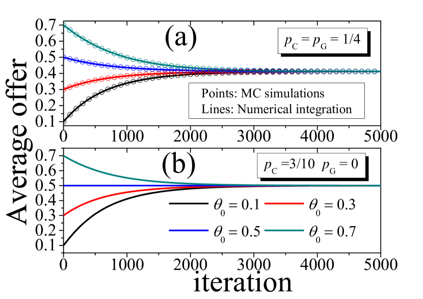
Figure 1: Evolution in time of the average offer for two different cases: the first one, the player adopts the strategies with probabilities $p_{C}=p_{G}=1/4$. Just for comparison, we also study the temporal evolution of the average offer for a case where the steady state is analytically expected to be fair: $\left\langle O_{\infty}\right\rangle=1/2$, we choose $p_{G}=0$ and $p_{C}=3/10$ for the sake of simplicity. In both cases we considered four different initial offers. In the first case, we can observe that a stationary fair offer is not obtained unlike the second situation. We observe that the initial condition is not important to the steady state of the average offer. The points in the first case show simple MC simulations performed to check the exact result.

In order to check such results, we obtain the temporal evolution of the average offer, by solving the temporal evolution equations, for two different cases: In the first one Fig. 1 (a), the player adopts the strategies with probabilities $p_{C}=p_{G}=1/4$. Thus, for a simple comparison, we also study the time evolution of the average offer for a case where the steady state is analytically expected to be fair: $\left\langle O_{\infty}\right\rangle=1/2$, we choose a particular case from Eq. 15: $p_{G}=0$ and $p_{C}=3/10$, for the sake of simplicity Fig. 1 (b). In both cases we considered four different initial offers. In the first case we can observe that the stationary fair offer is not observed, actually $\left\langle O_{\infty}\right\rangle\approx 0.4$, which differs on the second situation, where we check $\left\langle O_{\infty}\right\rangle\approx 0.5$. We observe that the initial condition is not important to the steady state of the average offer. The points in the first case correspond to simple MC simulations performed for checking the exact result.

Since we studied the evolution of the average offers, and we also verified the no dependence on initial offer, we can study in further detail the fairness condition predicted by Eq. 15. Thus, we solve Eq. 8 for all possible pairs $\left(p_{G},p_{C}\right)$, and the steady state average offer is drawn in Fig. 2.

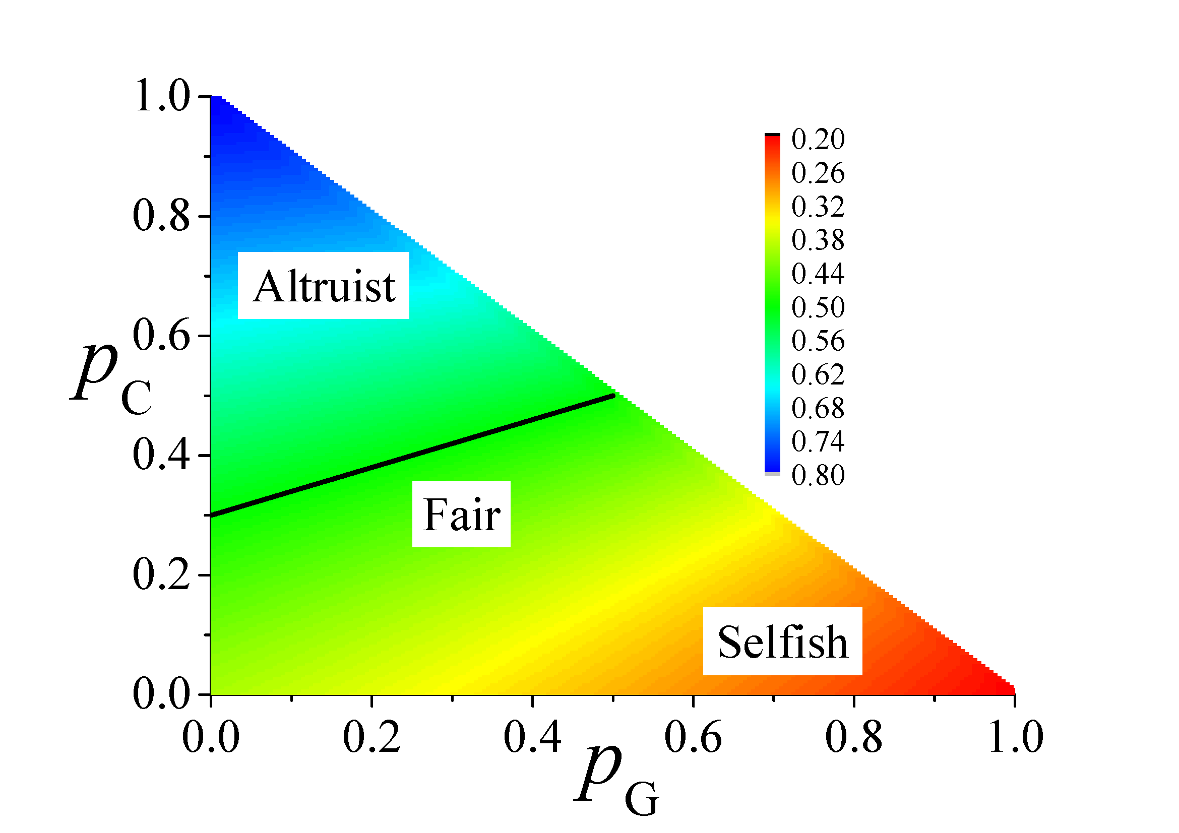
Figure 2: Colour map, steady state average offer for all possible pairs $(p_{G},p_{C}$). We have 3 distinct regions: altruist, fair, and selfish one. The dark line corresponds to exact fairness condition given by Eq. 15.

We can observe a complete description of the steady state average offer divided in three regions $\left\langle O_{\infty}\right\rangle<1/2$ (selfish region), $\left\langle O_{\infty}\right\rangle>1/2$ (altruist region), and finally $\left\langle O_{\infty}\right\rangle\approx 1/2$ (fair region) which contains the optimal fairness line given by Eq. 15.

3.2 Arbitrary $k$ and preliminary numerical investigations

It is important to observe that we can generalize Eq. 8 for an arbitrary coordination $k$. By following similar steps we can deduce that

$$\frac{d\left\langle O_{t}\right\rangle}{dt}=\left(2\sum_{m=0}^{k/2-1}\frac{k!\left\langle O_{t}\right\rangle^{m}(1-\left\langle O_{t}\right\rangle)^{k-m}}{m!(k-m)!}-1\right)p_{M}+\left(2(1-\left\langle O_{t}\right\rangle)^{k}-1\right)p_{G}+\left(1-2\left\langle O_{t}\right\rangle^{k}\right)p_{C}$$ (16)

Under stationary condition $\lim_{t\rightarrow\infty}\left\langle O_{t}\right\rangle=O_{\infty}=1/2$, we have for large $k$:

$$\begin{array}[]{lll}\sum_{m=0}^{k/2-1}\frac{k!\left\langle O_{t}\right\rangle^{m}(1-\left\langle O_{t}\right\rangle)^{k-m}}{m!(k-m)!}&=&\frac{1}{2^{k}}\sum_{m=0}^{k/2-1}\binom{k}{m}\\ &&\\ &\approx&\frac{2}{\sqrt{2\pi k}}\int_{0}^{k/2}dm\ e^{-\frac{(m-k/2)^{2}}{k/2}}\\ &&\\ &=&1/2\end{array}$$ (17)

and since $d\left\langle O_{t}\right\rangle/dt=0$, we have:

$$\frac{p_{G}}{p_{C}}=1$$ (18)

This result is very important but also intuitive. For any probability of a player acting as a moderate player, if you consider equal probabilities of acting as greedy and conservative, the player always leads to a fair offer when she/he plays with a large sample of players taking their decisions. This is expected, since as $k$ grows, the probability of a greedy player decreasing their offer is high, while the probability that a conservative player increases their offer is also high, if a player acts with equal probability for greedy and conservative, they must keep a fair steady state average offer, unlike in their moderate actions. This can be observed in Fig. 3 (a).

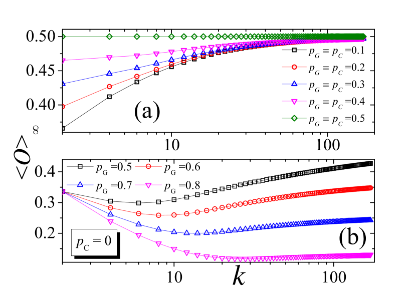
Figure 3: Steady state average offer as function of $k$. (a) Fairness occurs for high $k$ given a player that has equal probabilities to act as conservative and greedy, unlike in their moderate actions. (b) As the number of greedy players increases, the steady state average offer decreases, but there is a $k_{c}$ for that one and the steady state average offer is minimal.

This figure depicts the steady state average offer for different situations of $p_{G}=p_{C}$. However, for high $k$, the probability of the offer decreasing must be very small, and therefore we consider a particular, but interesting case $p_{C}=0$. So we study $\left\langle O_{\infty}\right\rangle$ as function of $k$ and the results is surprising. Although, $\left\langle O_{\infty}\right\rangle$ decreases as $p_{G}$ increases, for fixed $p_{G}$($p_{M}$), there is a $k_{C}$ such that $\left\langle O_{\infty}\right\rangle$ is minimal as shown in Fig. 3 (b). This non-monotonic behaviour in the static version can be explained taking into account a complex scenario. There is a competition of the parameters for the greedy actions. For intermediate $k$ and for good offers, a sequence of decreases on the offer can occur. At large $k$, it should be easy to find an accepting, but the previous catastrophic sequence of decreases makes the offers not so attractive and this balance between large $k$ and low offers must be the reason of the non-monotonic behaviour. On the other hand, moderate actions are not sensitive to $k$.

Since we have studied some interesting aspects of the static ultimatum game, in the next section we present the results of our MSSUG in the two dimensional lattice, exploring the points related to survival of strategies with introduction of mobility of the players.

4 Results II: Numerical simulations

We carried out numerical simulations of the MSSUG in two-dimensional lattices ($k=4$). Each player starts with one of three strategies, which are equally probable. Thus each player interacts with their four neighbours, acting as proposer. The responder acts analogously with respect to their four neighbours. The update is synchronous, i.e., after all interactions the strategies are updated for all players at once.

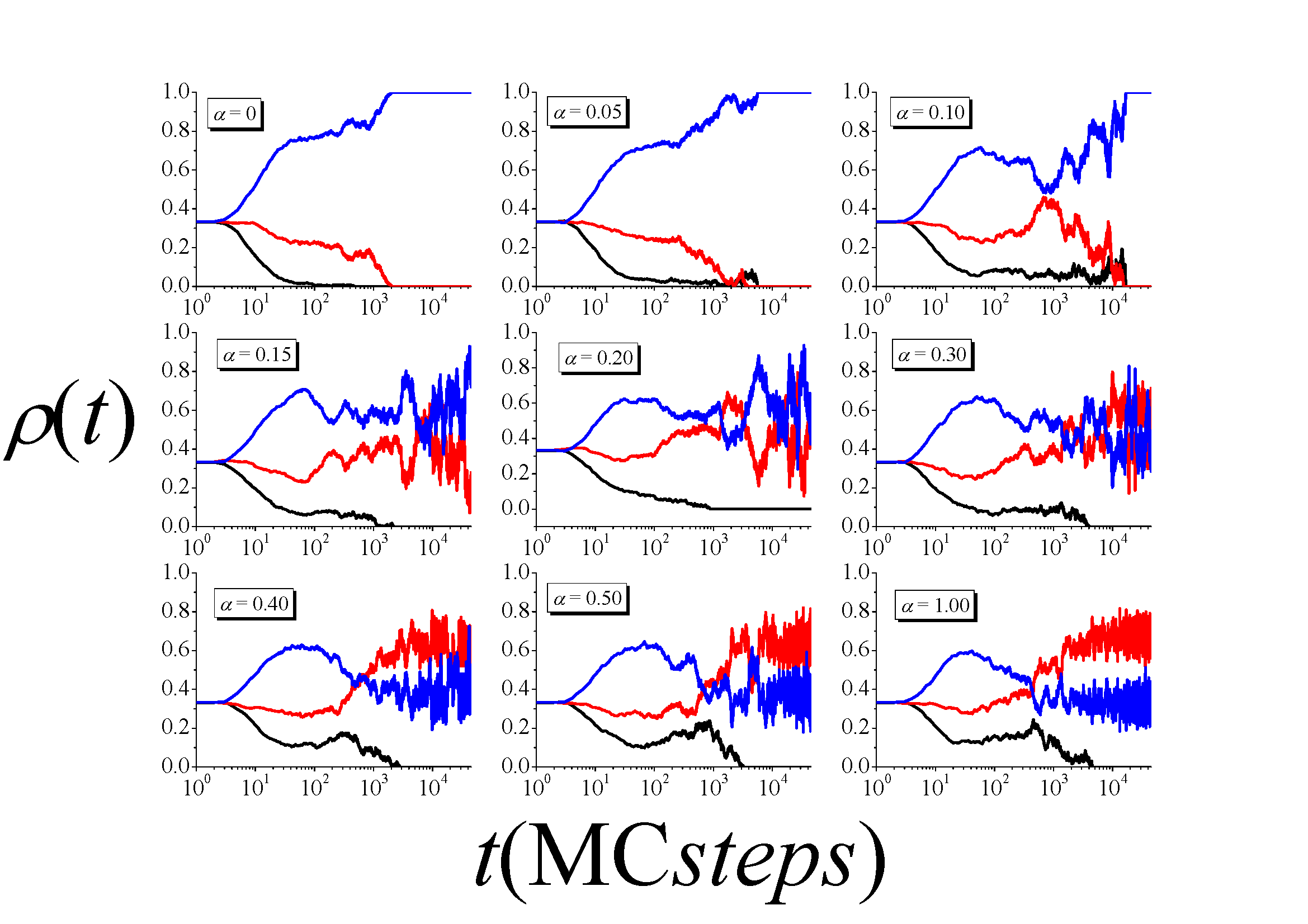
Figure 4: Density of strategies of the MSSUG for one only run.

We have monitored the density of strategies as function of time for different mobility values $\alpha$. First we consider the density of strategies for one only run as shown in Fig. 4. The results suggest that for low mobility, only conservative players survive. However as $\alpha$ increases the moderate players start increasing and the system pass by a coexistence between conservative and moderate players, which is followed by higher extension of survival of the greedy players that are always extinct. For $\alpha>\alpha_{c}$, with $0.2<\alpha_{c}<0.3$ there is a dominance of moderate players. Looking at $\alpha=0.3$, it is interesting to observe, considering one run only, that there is a region of coexistence between conservative and moderate players. It is interesting to observe a snapshot of spatial distribution of strategies which illustrate this coexistence as described in Fig. 5.

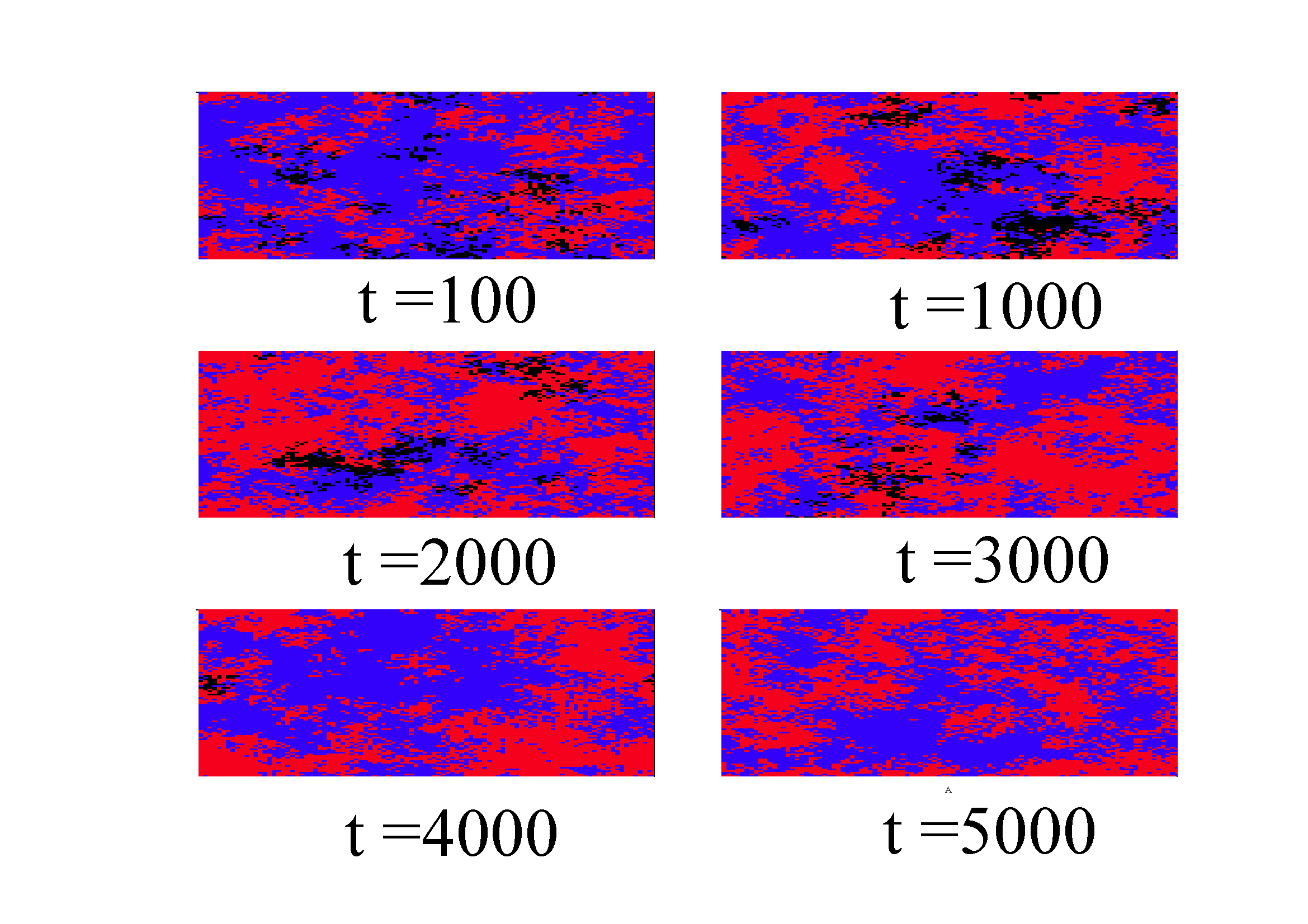
Figure 5: Snapshots of spatial distribution of strategies over time: black: greedy, red: moderate, and blue: conservative.

It is interesting to run again the experiment on the density of strategies considering many different runs. So, we consider the density average over $N_{run}=300$ different runs. The results are shown in Fig. 6.

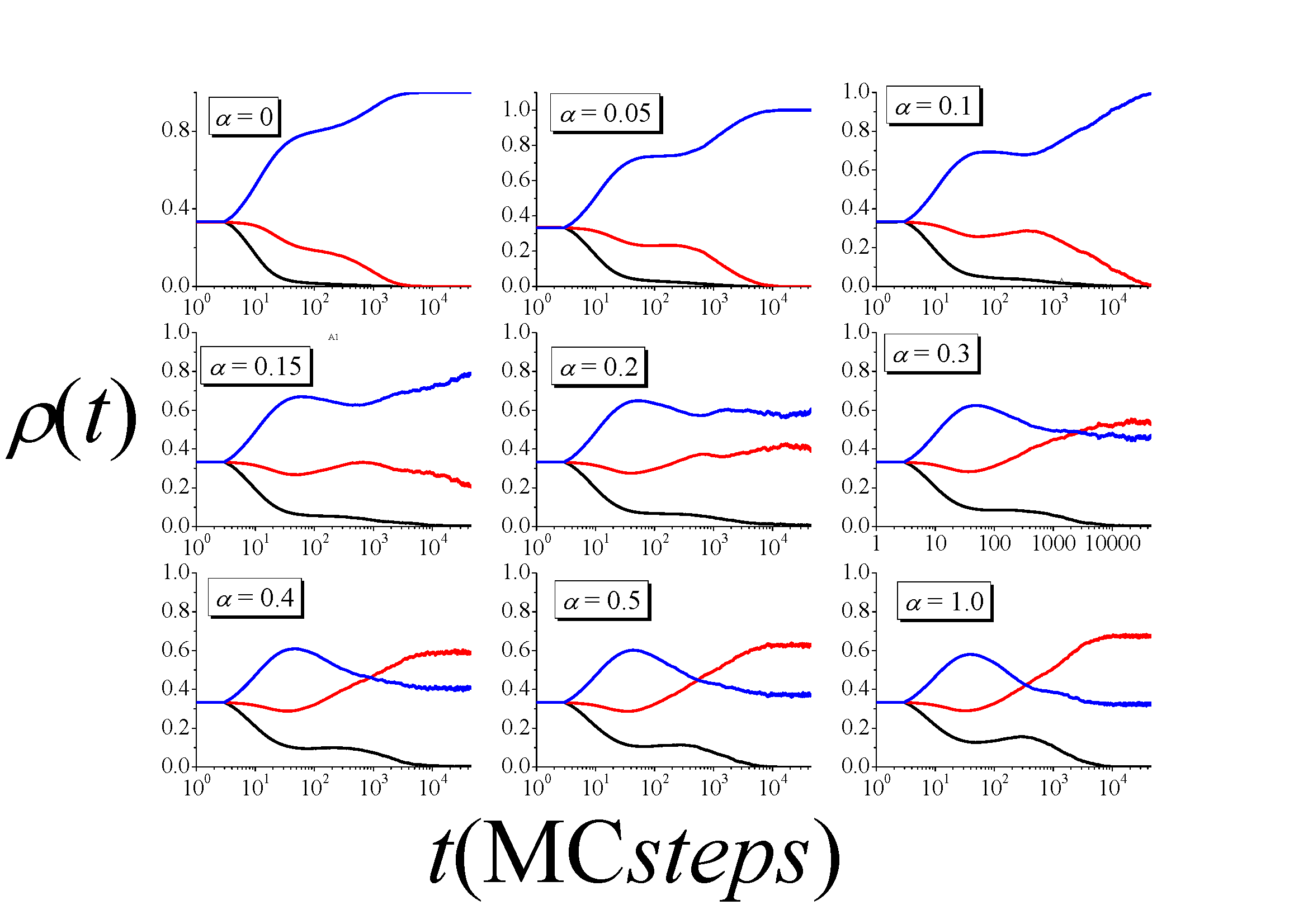
Figure 6: Density of strategies of the MSSUG averaged over 300 runs.

We can observe in more detail the inversion of dominance between conservative and moderate agents is indeed occurring the interval $[0.2,0.3]$, but it is interesting to refine the interval. Thus, we carried out simulations with $\Delta\alpha=0.01$, between $\alpha=0.2$ and $0.3$, and the inversion of dominance occurs exactly at $\alpha_{c}\approx 0.26$ as can be observed in Fig. 7. At this value we can see clearly a coexistence between the two strategies. A highlight of coexistence region is shown for $\alpha=0.26$.

Figure 7: Refinement of evolution of density of strategies. The inversion of dominance occurs for $\alpha\approx 0.26$, where we clearly has a coexistence between the conservative and moderate strategies.

If the mobility affects the dominant strategy of the agents, where the conservative agents dominate the moderate agents, for low mobility, while for high mobility the moderate strategy is the winner, this inverting the game, it is interesting to explore other parameters.

We thus choose four parameters:

1. Average payoff of proposers

   $$\left\langle P_{pr}(t)\right\rangle=\frac{1}{N\cdot N_{run}}\sum_{i=1}^{N}\sum_{j=1}^{N_{run}}P_{pr}(i,j;t)$$

   where $P_{pr}(i,j;t)$ corresponds to payoff of player $i$, only gaining as proposer, for sample $j$ in the simulation, at time $t.$

2. Average payoff of responders, which is similarly calculated as

   $$\left\langle P_{ac}(t)\right\rangle=\frac{1}{N\cdot N_{run}}\sum_{i=1}^{N}\sum_{j=1}^{N_{run}}P_{ac}(i,j;t)$$

   where $P_{ac}(i,j;t)$ corresponds to payoff of player $i$, only gaining as responder, for sample $j$ in the simulation, at time $t$.

By defining

$$P(i,j;t)=P_{pr}(i,j;t)+P_{ac}(i,j;t)$$

the total payoff of player $i$, for sample $j$ at time $t$ we have propose our third parameter:

1. Gini coefficient of total payoff, which is calculated as

   $$G(t)=\frac{1}{N_{run}}\sum_{j=1}^{N_{run}}G(j;t)$$

   where $0\leq G(j;t)\leq 1$ is the Gini coefficient [12] of the total payoff of the agents for sample $j$, which was already used by ourselves in the context of game theoretical models (see for example [6, 10]),

   $$G(j;t)=\frac{1}{(N-1)}\left[N+1-2\left(\frac{\sum_{i=1}^{N}(N+1-i)P(i,j;t)}{\sum_{i=1}^{N}P(i,j;t)}\right)\right]$$

   only to measure statistical heterogeneity of payoffs and no social context must be here explored, exactly as variance or other index, as for example the Pietra index [13]. And finally:

2. Average offer, which is calculated as

   $$\left\langle O(t)\right\rangle=\frac{1}{NN_{run}}\sum_{i=1}^{N}\sum_{j=1}^{N_{run}}O(i,j;t)$$

   where $O(i,j;t)$ is the offer of player $i$, for sample $j$, at time $t$.

And the question here is, what happens with these four parameters as a function of time? Moreover, what the is diffusion effect on them?

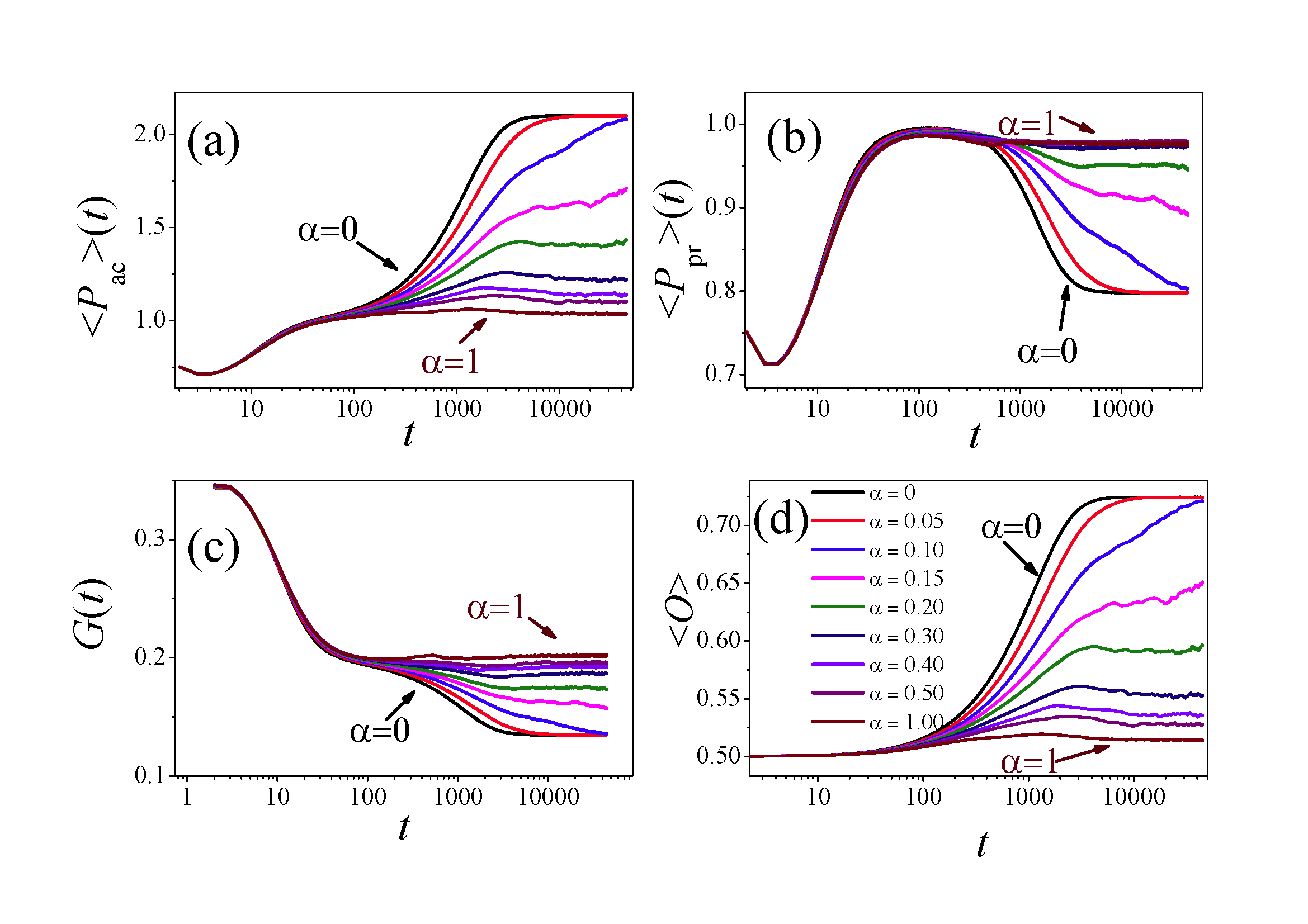
Figure 8: Temporal evolution of four parameters that describe the fluctuations on payoff and offer of agents under spatial diffusion effects. (a) Average payoff of responders, (b) Average payoff of proposers (c) Gini coefficient, and (d) Average offer.

As one can observe in Fig. 8 (a) the $\left\langle P_{ac}(t)\right\rangle$ increases as $t$ increases, but this increase is reduced as the mobility of agents grows. Differently, the mobility is good for the average payoff of the responders since $\left\langle P_{pr}(t)\right\rangle$ for large times gets higher, the higher $\alpha$ is, Fig. 8 (b). We know that low mobilities has a dominance of conservative players, while high mobilities shows the dominance of moderate ones. This is reflected by average offers, Fig. 8 (d), since conservative players require more levels of acceptance, the offer is increased to result in more acceptances, in this case there is a fixed point $O_{\infty}\approx 0.724$ for the average offer. However, as mobility increases, the average offer reaches fairer steady states. Finally, we analyse the Gini coefficient that decreases as function of time Fig. 8 (c). Mobility makes the heterogeneity of the payoff larger. The transition between the dominances is again observed, since the Gini coefficient has a fixed point ($G_{\infty}=0.135$) reached only for low mobilities (below $\alpha_{c}=0.26$). Thus the parameters show non-trivial behaviour of the game which corroborate the transition previously observed with density of strategies.

5 Conclusions

In this paper, we considered a reactive version of ultimatum game where the players regulate their offers and can assume three different strategies: greedy ($G$), moderate ($M$), and conservative ($C$) that differ on the level of greed. First, we show how to compose portfolios (probabilities of acting by choosing among these three strategies) that lead to fairer situations. Analytical results and a diagram representing this fairness is presented. Further, by including Darwinian and spacial aspects, we studied a multi-agent system of the model which shows that mobility has an important role over the dominance of strategies. We show that there exist a transition between dominances on the diffusion probability $\alpha$, for $\alpha<0.26$, $C\succ M$, while for $M\succ C$ for $\alpha>0.26$. A coexistence between these two strategies can be observed exactly in $\alpha=0.26$. This transition is reflected in four different parameters related to the offer, payoff, and the heterogeneity among the agents.

Acknowledgements – Roberto da Silva thanks CNPq for financial support under grant numbers: 311236/2018-9,and 424052/2018-0. Luis Lamb is partly supported by CNPq and by CAPES - Coordenação de Aperfeiçoamento de Pessoal de Nível Superior - Financed Code 001. This work was partly developed using the computational resources of Cluster Ada, IF-UFRGS.

References

References

- [1] W. Guth, R. Schmittberger, and B. Schwarze, J. Econ. Behav. Org. 24, 153 (1982)
- [2] K. Eriksson, P. Strimling, P. A. Andersson. T. Lindholm, J. Exp. Soc. Psychol. 69, 59-64 (2017)
- [3] A. Szolnoki, M. Perc, G. Szabo, Phys. Rev. Lett. 109, 078701-1 (2012).
- [4] S. Schuster, Scientific Reports 7, 5642 (2017)
- [5] E. Almeida, R. da Silva, A. S. Martinez, Physica A 412, 54 (2014)
- [6] R. da Silva, P. A. Valverde, L. C. Lamb, Commun. Nonlinear Sci. 36, 419 (2016).
- [7] R. da Silva, Mendeli H. Vainstein, Luis C. Lamb, Sandra D. Prado, Com. Phys. Comm. 184, 661-670 (2013)
- [8] R. da Silva, Mendeli H. Vainstein, S. Gonçalves, F. S. F. Paula, Phys. Rev. E. 88, 022136-022136-8 (2013)
- [9] R. da Silva, S. R. Dahmen, Physica A 398, 56-64 (2013)
- [10] R. da Silva, G. A. Kellermann, L. C. Lamb, J. Theor. Biol. 258, 208 (2009)
- [11] R. da Silva and G. A. Kellerman, Braz. J. Phys. 37, 1206 (2007).]
- [12] C. Gini, Econom. J. 31, 124 (1921).
- [13] I. I. Eliazar, I. M. Sokolov, Physica A 389, 117–125 (2010)