Probing cosmic acceleration by strong gravitational lensing systems

Abstract

Recently, some divergent conclusions about cosmic acceleration were obtained using type Ia supernovae (SNe Ia), with opposite assumptions on the intrinsic luminosity evolution. In this paper, we use strong gravitational lensing systems to probe the cosmic acceleration. Since the theory of strong gravitational lensing is established certainly, and the Einstein radius is determined by stable cosmic geometry. We study two cosmological models, $\Lambda$CDM and power-law models, through 152 strong gravitational lensing systems, incorporating with 30 Hubble parameters $H(z)$ and 11 baryon acoustic oscillation (BAO) measurements. Bayesian evidence are introduced to make a one-on-one comparison between cosmological models. Basing on Bayes factors $\ln B$ of flat $\Lambda$CDM versus power-law and $R_{h}=ct$ models are $\ln B>5$, we find that the flat $\Lambda$CDM is strongly supported by the combination of the datasets. Namely, an accelerating cosmology with non power-law expansion is preferred by our numeration.

1 Introduction

As a standard cosmological model, the $\Lambda$CDM is widely accepted basing on some remarkable observations, including type Ia supernovae (SNe Ia) (Riess et al., 1998; Perlmutter et al., 1999), cosmic microwave background (CMB) (Bennett et al., 2011, 2013; Planck Collaboration et al., 2014, 2016a), baryon acoustic oscillations (BAOs) (Eisenstein et al., 2005) and gamma-ray bursts (Wang et al., 2015). But many imperfections of $\Lambda$CDM are also needed to be faced, including the fine tuning problem and the cosmic coincidence problem (Weinberg, 1989; Zlatev et al., 1999). Additionally, the capability of using SNe Ia to prove cosmic acceleration is under doubt recently (Nielsen et al., 2016; Shariff et al., 2016).

In a bunch of cosmological models, power-law cosmology was proposed with an assumption that the scale factor varies as $a(t)\propto t^{n}$ (Dolgov, 1997; Dolgov et al., 2014). Many works have devoted into the study of power-law cosmology. Melia (2007) and Melia & Shevchuk (2012) made a special situation of this model, where a non-accelerated cosmology was considered as $a(t)\propto t$. Namely, the cosmic horizon $R_{h}$ equals to the light-travel time distance. By using different kinds of observations, this non-accelerated power-law cosmology was found to be preferred (Melia & Maier, 2013; Melia & McClintock, 2015; Melia et al., 2015; Tutusaus et al., 2017). However this model was also perceived to be against to SNe Ia and BAO data (Bilicki & Seikel, 2012; Dolgov et al., 2014; Shafer et al., 2015; Haridasu et al., 2017). Progress has been made in probing power-law cosmology (Sethi et al., 2005; Dev et al., 2008; Zhu et al., 2008; Dolgov et al., 2014; Yu & Wang, 2014). Nevertheless, many researches also questioned the possibility of replacing $\Lambda$CDM by power-law cosmology (Kumar, 2012; Cárdenas & Herrera, 2015; Rani et al., 2015; Yuan & Wang, 2015; Tutusaus et al., 2016; Haridasu et al., 2017; Lin et al., 2017).

Treating SNe Ia as standard candles is broadly used in probing cosmology, and this method is required to be deliberately considered according to some literature recently. Tutusaus et al. (2017) found that SNe Ia are consistent with a non-accelerated universe with assumption that supernovae intrinsic luminosity depends on the redshift. Considering the independence of supernovae intrinsic luminosity on redshift, Lin et al. (2017) got a contradictory conclusion with Tutusaus et al. (2017). Nielsen et al. (2016) presented an improved maximum-likelihood procedure to reanalyze the SNe Ia dataset with improvement of precision and scale. They found the marginal evidence of an accelerated expansion cosmology which was widely accepted before. A new method called BAyesian HierArchical Modeling for the Analysis of Supernova cosmology (BAHAMAS) was introduced by Shariff et al. (2016), and they found a sharp dropping of the color correction parameter value $\beta$ with redshift. Color correction parameter is roughly constrained over all redshift through empirical period-luminosity relation. However, some voices (Rubin & Hayden, 2016; Ringermacher & Mead, 2016) have grown to demonstrate an accelerated cosmology and pointed some inappropriatenesses in Nielsen et al. (2016). While using SNe Ia, a set of complex parameters are involved to be constrained by empirical period-luminosity relation of Cepheid variables (Phillips, 1993). Several uncertainties of this relation are also needed to be prudently studied, e.g., the dependence of absolute B band magnitude $M_{B}$ on redshift (Holz & Linder, 2005), the effects of systematic errors (Freedman & Madore, 2010; Ruiz et al., 2012), and poor uniformity of SNe Ia in various galaxy environment (Gilfanov & Bogdán, 2010). When probing cosmic acceleration, all the considerations above trigger us to use other observations. We choose strong gravitational lensing systems which are purely geometrically effected and endorsed by certain theory.

Walsh et al. (1979) discovered the first strong gravitational lensing Q0957+561. Decades years later, strong gravitational lensing systems are widely used in cosmology (Zhu & Sereno, 2008; Wang & Dai, 2011; Cao et al., 2012; Wei et al., 2014; Liao et al., 2016; Leaf & Melia, 2018; Yu & Wang, 2018; Wang & Wang, 2018). Basing on the Einstein radius formulation, the Hubble constant is eliminated through distance ratio. This may avoid some undiscovered relationship between Hubble constant and other observed values, e.g., the absolute magnitude $M_{B}$ of SNe Ia. Considering that the strong gravitational lensing systems may show of lacking capability to constrain $\Omega_{m}$ for $\Lambda$CDM (Biesiada et al., 2010), other kinds of data are combined to constrain parameters precisely in this paper.

In our work, we focus on using strong gravitational lensing systems, Hubble parameters $H(z)$ and BAOs to compare cosmological models through Markov chain Monte Carlo (MCMC) method. We also pick a favorable cosmological model quantitatively through Bayesian evidence.

This paper is organized as follows. Two cosmological models will be briefly introduced in section 2. All kinds of data and methodology are given in section 3. The results of MCMC simulation are presented in section 4. Conclusions are given in section 5.

2 Cosmological Models

In this section, we briefly present two cosmological models in our analysis, including $\Lambda$CDM and power-law model.

2.1 $\Lambda$CDM model

With an assumption of isotropy and homogeneity of the universe, the Hubble parameter can be derived as

$$\left(\frac{H}{H_{0}}\right)^{2}=\Omega_{r}a^{-4}+\Omega_{m}a^{-3}+\Omega_{k}a^{-2}+\Omega_{\Lambda},$$ (1)

where $\Omega_{r}$, $\Omega_{\Lambda}$, $\Omega_{m}$ and $\Omega_{k}$ represent radiation, dark energy, matter and curvature of the universe, respectively. $\Omega_{r}$ is fixed as $\Omega_{r}=0$ in our analysis, basing on the radiation of universe is observed to be negligible in present day. $\Omega_{m}+\Omega_{k}+\Omega_{\Lambda}=1$ represent the total density which is dimensionless. Using $a=(1+z)^{-1}$, eq.(1) can be derived into

$$H(z)=H_{0}[\Omega_{m}(1+z)^{3}+\Omega_{k}(1+z)^{2}+\Omega_{\Lambda}]^{1/2}.$$ (2)

We consider a flat-$\Lambda$CDM model and a $\Lambda$CDM with curvature (denoted as curve-$\Lambda$CDM). Through fixing $\Omega_{k}=0$ for flat-$\Lambda$CDM, eq.(2) can be written as

$$H(z)=H_{0}[\Omega_{m}(1+z)^{3}+\Omega_{\Lambda}]^{1/2}.$$ (3)

2.2 Power-law model

Power-law cosmology (denoted as PL) is derived from the power-law relation between the scale factor and proper time as

$$a(t)=\left(\frac{t}{t_{0}}\right)^{n}.$$ (4)

By using $H\equiv{\dot{a(t)}}/{a(t)}$ and $a=(1+z)^{-1}$, one can easily obtain Hubble parameter function as

$$H(z)=H_{0}(1+z)^{\frac{1}{n}},$$ (5)

where $H_{0}=n/t_{0}$.

The $R_{h}=ct$ can be considered as a unique circumstance of power-law model, in which $n=1$. The gravitational horizon scale is handled as $R_{h}=ct$. Taking $n=1$ into eq.(5), we can obtain the Hubble parameter given as

$$H(z)=H_{0}(1+z).$$ (6)

The deceleration parameter of $R_{h}=ct$ model is $q=0$, which expresses a universe expanding steadily. $n>1$ and $n<1$ represent an accelerated and a decelerated universe respectively, according to the relation $q=1/n-1$.

After reviewing these two cosmological models, one can derive the comoving distance for each model as below (Hogg, 1999). The comoving distance for flat-$\Lambda$CDM is written as

$$D_{C}=\frac{c}{H_{0}}\int_{0}^{z}{\frac{1}{\sqrt{\Omega_{m}(1+z)^{3}+\Omega_{\Lambda}}}}dz.$$ (7)

For curve-$\Lambda$CDM the comoving distance is based on curvature ${\Omega}_{k}$,

$$D_{C}=\left\{\begin{array}[]{ll}\frac{c}{\sqrt{{\Omega}_{k}}}\sinh{\left(\int_{0}^{z}{\frac{1}{H(z)}}dz\cdot\sqrt{{\Omega}_{k}}\right)}&{\Omega}_{k}>0\\ \\ {c}\int_{0}^{z}{\frac{1}{H(z)}}dz&{\Omega}_{k}=0\\ \\ \frac{c}{\sqrt{\left|{\Omega}_{k}\right|}}\sin{\left(\int_{0}^{z}{\frac{1}{H(z)}}dz\cdot\sqrt{\left|{\Omega}_{k}\right|}\right)}&{\Omega}_{k}<0\end{array}\right.,$$ (8)

where $H(z)$ is from eq.(2). For power-law model $(n\neq 1)$ we have

$$D_{C}=\frac{c}{H_{0}}\frac{\left(1+z\right)^{1-\frac{1}{n}}-1}{1-\frac{1}{n}}.$$ (9)

When $n=1$ namely $R_{h}=ct$ model, the function can be derived as

$$D_{C}=\frac{c}{H_{0}}\ln\left(1+z\right).$$ (10)

The angular diameter distance for each model can be written as

$$D_{A}=\frac{D_{C}}{\left(1+z\right)}.$$ (11)

3 Data and Methodology

In this section, we present data including strong gravitational lensing systems, $H(z)$, and BAO. The methods which we treat to various data will be illustrated here.

3.1 Strong lensing systems

Strong gravitational lensing system has become a useful and vital tool in probing cosmology. From the first lensing system has been discovered, there are abundant projects searching for lensing systems, including Sloan Lens ACS (SLACS), BOSS Emission-Line Lens Survey (BELLS), etc. Approximated by singular isothermal sphere (SIS) model or singular isothermal ellipsoid (SIE) model, the Einstein radius can be obtained by measuring the foreground image of Einstein rings and can be expressed through the formula as

$$\frac{D^{ls}_{A}}{D^{s}_{A}}=\frac{\theta_{E}\;c^{2}}{4\pi\sigma^{2}_{SIS}}=\mathcal{D}^{obs},$$ (12)

where $c$ is the speed of light and $\theta_{E}$ represents Einstein radius. $D^{ls}_{A}$ and $D^{s}_{A}$ are angular diameter distances from lensing to source and observer to source respectively.

White & Davis (1996) found that the dynamical temperature of dark matter halos is larger than measured stellar velocity dispersion, which hints that the velocity dispersion $\sigma_{SIS}$ in eq.(12) may not be equal to observed stellar velocity dispersion $\sigma_{ap}$. Cao et al. (2015) assumed that the mass of strong lensing systems is distributed spherically and symmetrically. In their work power-law index $\gamma$ of massive elliptical galaxies is treated as a free parameter, and $\mathcal{D}^{obs}$ can be derived as

$$\mathcal{D}^{obs}=\frac{\theta_{E}\;c^{2}}{4\pi\sigma^{2}_{ap}}f\left(\theta_{E},\theta_{ap},\gamma\right).$$ (13)

$f\left(\theta_{E},\theta_{ap},\gamma\right)$ is a complex function related to Einstein radius $\theta_{E}$, aperture of certain lensing surveys $\theta_{ap}$, and power-law index $\gamma$. But this method may show poor sensitivity to cosmological parameters (Jie et al., 2016).

Another simple method is replacing $\sigma_{SIS}$ of eq.(12) by $\sigma_{SIS}=f_{e}\sigma_{ap}$ (Kochanek, 1992; Ofek et al., 2003). As a phenomenological free parameter, $f_{e}$ accounts the systematic errors caused by taking $\sigma_{ap}$ as $\sigma_{SIS}$. Unlike Leaf & Melia (2018) have done recently, free parameter $f_{e}$ is introduced to calculate $\mathcal{D}^{obs}$. Therefore, $\mathcal{D}^{obs}>1$ can not be used to exclude unphysical observed lensing systems, which has been used in Leaf & Melia (2018).

Moreover, in order to correct observed stellar velocity dispersion into a circular aperture of radius, $\sigma_{0}=\sigma_{ap}\left(\theta_{eff}/\left(2\theta_{ap}\right)\right)^{-0.04}$ can be used (Jorgensen et al., 1995a, b). $\theta_{eff}$ represents the effective radius, which is achieved by fitting de Vaucouleurs model (de Vaucouleurs, 1948). Cao et al. (2015) replaced $\sigma_{ap}$ of eq.(13) by $\sigma_{0}$. Replacing $\sigma_{SIS}$ directly by $\sigma_{0}$ in eq.(12) may not be a proper treatment, which has been used by Leaf & Melia (2018). Because $\sigma_{0}$ just changes slightly from $\sigma_{ap}$ (Cao et al., 2015).

In order to exclude other systematic errors and unknown uncertainties introduced from lensing model fitting effect, we use $\sigma_{SIS}=f_{e}\sigma_{ap}$ in this paper, which has been widely used (Cao et al., 2012; Liao et al., 2016; Li et al., 2017; Xia et al., 2017).

From eq.(12), we can obtain the angular diameter distance ratio observed from lensing surveys $\mathcal{D}^{obs}$. The uncertainty of $\mathcal{D}^{obs}$ can be written as

$$\sigma_{\mathcal{D}^{obs}}=\mathcal{D}^{obs}\sqrt{\left(\frac{\sigma_{\theta_{E}}}{\theta_{E}}\right)^{2}+4\left(\frac{\sigma_{\sigma_{SIS}}}{\sigma_{SIS}}\right)^{2}}.$$ (14)

Following the approach taken by Grillo et al. (2008), we take uncertainties of Einstein radius as $\sigma_{\theta_{E}}=0.05\theta_{E}$. The theoretical angular diameter distance ratio $\mathcal{D}^{th}$ can be derived from eqs.(7) $\sim$ (11). The angular diameter distance is written as

$$D_{A}^{ls}=\frac{D_{C}^{ls}}{1+z_{s}}.$$ (15)

Easily, $\mathcal{D}^{th}$ has the relation

$$\mathcal{D}^{th}=\frac{D_{C}^{ls}}{D_{C}^{s}},$$ (16)

where $D_{C}^{ls}=D_{C}^{s}-D_{C}^{l}$ for flat-$\Lambda$CDM, PL model and $R_{h}=ct$ model. For curve-$\Lambda$CDM, it is unnecessary to derive an equation relating $D_{C}^{ls}$, $D_{C}^{l}$, and $D_{C}^{s}$, but to substitute the range of integration in eq.(8) from $0$ to $z$ into $z_{l}$ to $z_{s}$ (Räsänen et al., 2015).

$f_{e}$ as a free parameter in eq.(12) is required to be fitted simultaneously. Naturally, the mean values of parameters can be obtained by minimizing

$$\chi^{2}_{SL}=\sum_{i=1}^{n}{\frac{\left(\mathcal{D}^{th}-\mathcal{D}^{obs}\right)^{2}}{\sigma^{2}_{\mathcal{D}^{obs}}}}.$$ (17)

The likelihood is $\mathcal{L}_{SL}\propto\exp(-\chi^{2}_{SL}/2)$.

The idea of reducing systematic errors requires a dataset comprehending as much high-quality data as possible. We utilize 152 strong gravitational lensing systems in our analysis. 118 strong gravitational lensing systems are taken from catalog of Cao et al. (2015). The catalog was assembled from the Sloan Lens ACS Survey (SLACS), BOSS emission-line lens survey (BELLS), Lens Structure and Dynamics (LSD), and Strong Lensing Legacy Survey (SL2S). Further more, 34 new strong gravitational lensing systems are carefully selected and used in this work. 7 reliable BELLS data with much higher source redshifts are selected cautiously from Shu et al. (2016). Actually, there are 17 grade-A lenses listed in Shu et al. (2016). To be specific, five systems require special model-fitting treatments, four systems show significantly larger relative deviations of the Einstein radius, and one system do not meet the selection thresholds. These 10 systems are excluded in order to get rid of some unknown systematic errors imported by any model fitting effect. 27 SLACS data are chosen from 40 grade-A lenses listed in Shu et al. (2017). In their work, a parameter $\chi^{2}/dof$ is achieved, which represents the goodness of fitting for SIE model. 27 lenses are filtrated carefully, whose $\chi^{2}/dof$ is within the interval of $1\sigma$ around the constrained value $\chi^{2}/dof=1$. Apart from 118 strong gravitational lensing systems, the new 34 data are listed in Table 1.

3.2 Hubble parameter H(z)

By using cosmic chronometers approach (Jimenez & Loeb, 2002), the Hubble parameter is measured independently of cosmological models. Through this approach one can directly constrain the expansion history of the universe, and avoid any integrated distance measurements over redshift like SNe Ia and BAOs.

In our work we take 30 $H(z)$ data from Moresco et al. (2016) over 25 data listed in Melia & McClintock (2015). Note that all 30 $H(z)$ data are cosmological-model independent. The $\chi_{H(z)}^{2}$ for Hubble parameters is given by

$$\chi^{2}_{H(z)}=\sum_{i=1}^{n}{\frac{\left({H(z)}^{th}-{H(z)}^{obs}\right)^{2}}{\sigma^{2}_{{H(z)}^{obs}}}},$$ (18)

where $H(z)^{th}$ is the theoretical value of Hubble parameter. The likelihood is $\mathcal{L}_{H(z)}\propto\exp(-\chi^{2}_{H(z)}/2)$.

3.3 Baryon acoustic oscillations

As a model-independent standard ruler, BAO is a practical tool in probing cosmology. Through measuring the comoving sound horizon of the baryon drag epoch at different redshifts (Eisenstein et al., 2005), the sound horizon size at the end of the drag era $z_{d}$ is written as

$${r}_{d}=r_{s}(z_{d})=\int_{{z}_{d}}^{\infty}{\frac{{c}_{s}(z)dz}{H(z)}},$$ (19)

where $c_{s}$ is the speed of sound. $r_{d}$ may relate more to early universe, from which we can’t get enough information. Besides $\Lambda$CDM, other cosmological models may not have a compatible function of $r_{d}$ (Verde et al., 2017a). Considering our work focus on different cosmological models, we regard $r_{d}$ as a free parameter following. BAO measures the ratio of comoving sound horizon and the distance scale (Eisenstein et al., 2005) given as

$$R(z)=\frac{r_{d}}{D_{V}},$$ (20)

and $D_{V}$ is defined as

$${D}_{V}(z)\equiv\left[D_{C}^{2}(z)\frac{cz}{H(z)}\right]^{\frac{1}{3}},$$ (21)

where comoving distance $D_{C}$ and Hubble parameter $H(z)$ are both defined in Section 2.

We use 11 BAO measurements from different surveys, which are listed in Table 2. In order to avoid importing BAO data at same redshifts repeatedly, we use the latest measurements of each redshift. Also we avoid importing BAOs with correlated surveys as far as possible (Yu, Ratra & Wang, 2018). To be specific, BAOs from 6dFGS, SDSS DR7, BOSS DR12, BOSS DR14 and Ly-$\alpha$ are uncorrelated with each other. Actually, there are two methods of Ly$\alpha$-forest. One method is Ly$\alpha$ auto-correlation, and the other is Ly$\alpha$ cross-correlation. Here, we use the BAO of combining both these two methods from du Mas des Bourboux et al. (2017), who have combined their measurement by cross-correlation at redshift 2.4 and auto-correlation at redshift 2.33 (Bautista et al., 2017) together.

Basically, there are two main analytical methods of measuring BAOs. One is anisotropic galaxy clustering measurement which constrains comoving distance $D_{M}(z)$ in the transverse direction and Hubble parameter $H(z)$ along line-of-sight. In this work, $D_{M}$ equals to $D_{C}$ which has been defined for different cosmological models in section 2. This method is also known as an application of Alcock-Paczynski effect (Alcock & Paczynski, 1979). The other is spherically averaged clustering which constrains volume-averaged distance $D_{V}$ (Eisenstein et al., 2005).

Results of both measurements are all used in this work. The original data of each BAO are listed in Table 2. Specially, for different BAO measurements at $z=0.38,0.51,0.61$, measurements in the transverse direction and along line-of-sight are both included (following e.g. Wojtak, & Prada, 2017; Lemos et al., 2018; Ryan et al., 2018). So we take covariance matrix from Alam et al. (2017) into our calculation. For BAO at $z=2.4$ (du Mas des Bourboux et al., 2017), we also take a small covariance matrix.

The $\chi^{2}_{BAO}$ is given by

$$\chi^{2}_{BAO}=({\bm{V}^{obs}-\bm{V}^{th}})\bm{C}^{-1}(\bm{V}^{obs}-\bm{V}^{th})^{T},$$ (22)

where ${\bm{V}^{obs}}$ and ${\bm{V}^{th}}$ are observed measurements and theoretical values corresponding to second column of Table 2. $\bm{C}^{-1}$ is inverse covariance matrix of the observed variables. For BAOs at $z=0.38,0.51,0.61$, the corresponding elements of inverse covariance matrix in eq.(22) are:

$$\begin{array}[]{lll}c_{44}=2.88,&c_{45}=-1.24,&c_{46}=0.16,\\ c_{47}=-6.76,&c_{48}=3.61,&c_{49}=-0.58,\\ c_{55}=2.49,&c_{56}=-0.90,&c_{57}=2.01,\\ c_{58}=-7.14,&c_{59}=3.21,&c_{66}=1.40,\\ c_{67}=-0.66,&c_{68}=2.28,&c_{69}=-4.82,\\ c_{77}=380.85,&c_{78}=-192.93,&c_{79}=18.60,\\ c_{88}=510.88,&c_{89}=-210.83,&c_{99}=339.81.\end{array}$$

For BAO at $z=2.4$, the inverse covariance matrix is:

$$\begin{array}[]{lll}c_{1010}=799.17,&c_{1011}=1578.\end{array}$$

These elements should be multiplied by $10^{-3}$. Here, $c_{ij}=c_{ji}\;\left(i\neq j\right)$. For the rest of elements, we have $c_{ii}=1/\sigma_{i}^{2}$ and $c_{ij}=c_{ji}=0\;\left(i\neq j\right)$, where $\sigma_{i}^{2}$ is error for BAO measurements.

The likelihood is $\mathcal{L}_{BAO}\propto\exp(-\chi^{2}_{BAO}/2)$.

In our work, we constrain the parameters for each cosmological model by using different combinations of these three kinds of data. The free parameters $f_{e}$ and $r_{d}$ are also needed to be constrained simultaneously. The three different datasets and corresponding total likelihoods are listed as below.

• Strong gravitational lensing system only (hereafter SL): $\mathcal{L}_{SL}$

• Strong gravitational lensing system and $H(z)$ (hereafter SL+$H(z)$): $\mathcal{L}_{SL}\cdot\mathcal{L}_{H(z)}$

• Strong gravitational lensing system, $H(z)$ and BAO (hereafter SL+$H(z)$+BAO) $\mathcal{L}_{SL}\cdot\mathcal{L}_{H(z)}\cdot\mathcal{L}_{BAO}$

It should be noted that the maximum likelihood method can be achieved by Bayesian approach (e.g. D’Agostini, 2005; Hogg et al., 2010) or frequentist approach (e.g. Planck Collaboration et al., 2016b). In this work, we use maximum likelihood method basing on Bayesian approach. Using information criteria may not be an excellent choice, because the information criteria derived from Bayesian approach may be a little different from the true values of comparison criteria. Also, the information criteria do not include the prior probability distributions into comparison (Liddle, 2007). So, we then introduce Bayesian evidence (Liddle, 2007; Trotta, 2008) as model comparison criteria. The Bayesian evidence is defined as

$$E\equiv\int{\mathcal{L}(\theta)}P(\theta)\rm d\theta,$$ (23)

where $\theta$ represents parameters of models. $\mathcal{L}(\theta)$ is likelihood function, and $P(\theta)$ gives priors distribution of parameters. The Bayes factor in natural logarithm $\ln B$ can be derived as

$$\ln B=\ln E_{fid}-\ln E_{\alpha},$$ (24)

where $fid$ represents flat-$\Lambda$CDM which we fix as the fiducial model, and ${\alpha}$ represent other models in one-on-one comparison. The $\ln E$ represents Bayesian evidence (eq.23) in natural logarithm. The preference strength for flat-$\Lambda$CDM can be described as weak, moderate or strong, according to $\ln B>1.0,$ $2.5$ or $5.0$ (Trotta, 2008). Naturally, a negative $\ln B$ value represents flat-$\Lambda$CDM is not favored.

4 Results

We use an open source python package emcee (Foreman-Mackey et al., 2013) to constrain cosmological parameters through Markov chain Monte Carlo method. The python package nestle is used to calculate Bayesian evidence through nested sampling algorithm (Skilling, 2004). The Hubble constant $H_{0}$ and the comoving sound horizon $r_{d}$ are replaced by $h_{0}=H_{0}/100$ and $r_{*}=r_{d}/100$ in our numeration. Uniform distributions of prior probabilities for the parameters are assumed: $P(\Omega_{m})=U[0,1]$, $P(\Omega_{k})=U[-1,1]$, $P(n)=U[0,2]$, $P(f_{e})=U[0.5,1.5]$, and $P(h_{0})=U[0.5,1]$. When we constrain parameters of curve-$\Lambda$CDM, we add another prior $P(\Omega_{\Lambda})=U[0.6,0.8]$ to constrain $\Omega_{k}$ more precisely.

Verde et al. (2017b) constrained the early cosmology from current CMB observations without any assumptions of late-time cosmology. They model-independently measured the value of $r_{d}$ as $r_{d}=147.4\pm 0.7$ Mpc. Because BAOs are sensitive to $r_{d}$ and $H_{0}$, BAOs may not be able to constrain both $r_{d}$ and $H_{0}$ at same time. So, we set uniform prior of $r_{*}$ as $P(r_{*})=U[1,2]$ or Gaussian prios $r_{*}=1.474\pm 0.007$ when importing BAO measurements, respectively. Meanwhile, we set $\Omega_{\Lambda}$ as a free parameter in curve-$\Lambda$CDM by only setting uniform priors on $\Omega_{k}$ and $\Omega_{m}$.

Due to the poor quality of SL data, it may not properly constrain cosmological parameters. In Table 3, we only list the mean value and 1$\sigma$ limits of each parameter. According to Bayes factors listed in Table 4, flat-$\Lambda$CDM is slightly favored rather than $R_{h}=ct$, according to $\ln B>2.5$. However, Leaf & Melia (2018) found $R_{h}=ct$ model is preferred over $\Lambda$CDM model. The reason is that they excluded some SL systems, as we discuss in section 3.

Then another dataset SL+$H(z)$ is imported in our analysis. The fitting results are listed in the second four rows of Table 3. By comparing the result only fitted by SL, one can easily find that the accuracies of $\Omega_{m}$ and $n$ are both improved dramatically. There is no significant variation of the free parameter $f_{e}$ for different models. Till now, we believe that through combination of different datasets, the accuracy of fitting will be enhanced significantly. By comparing Bayes factors in Table 4, it is impossible to rule out some models from flat-$\Lambda$CDM. Only PL can be ruled out, according to $\ln B>2.5$.

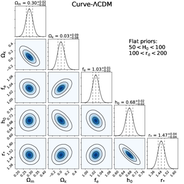
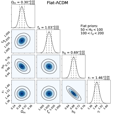
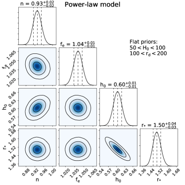
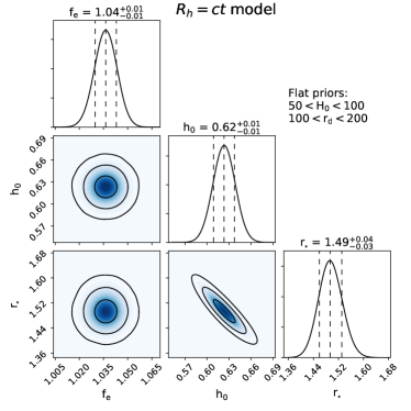
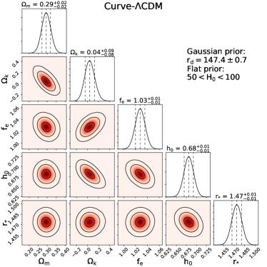
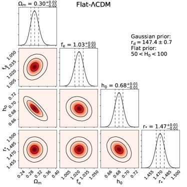
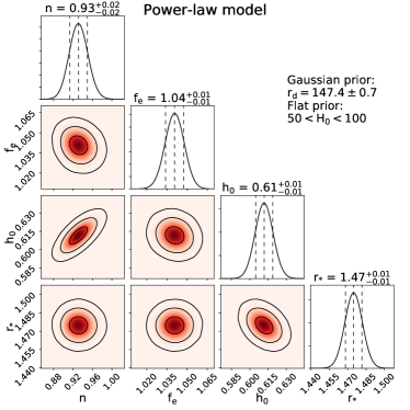
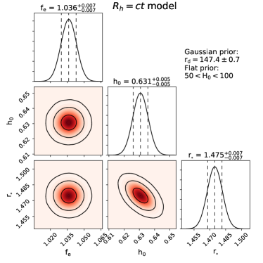
Next, the last dataset SL+$H(z)$+BAO is applied to our work. Firstly, we use a flat prior of $r_{d}$ , and our calculation gives optimized fitting results, which are listed in table 3 (called case 1). To be specific, the top-left panel of Figure 1 reveals the results of MCMC simulation for curve-$\Lambda$CDM. The mean values are $\Omega_{m}=0.30\pm 0.02$, $\Omega_{k}=0.03\pm 0.09$, $h_{0}=0.68\pm 0.02$, and $r_{*}=1.47\pm 0.04$. The value of $\Omega_{k}$ is consistent with zero at $1\sigma$ confidence interval. The fitting results of flat-$\Lambda$CDM are shown in top-right panel of Figure 1, where $\Omega_{m}=0.30\pm 0.02$, $h_{0}=0.69\pm 0.02$, and $r_{*}=1.46\pm 0.04$. For these two models, $r_{*}$ and $h_{0}$ are consistent. In the bottom-left panel of Figure 1, constraints on PL model are $n=0.93\pm 0.02$, $h_{0}=0.60\pm 0.01$, and $r_{*}=1.50\pm 0.04$. For $R_{h}=ct$ model, the bottom-right panel of Figure 1 reveals the mean values as $h_{0}=0.62\pm 0.01$, and $r_{*}=1.49\pm 0.04$. Values of $r_{d}=100r_{*}$ for these two models are a little bit larger than $r_{d}$ measurement as $r_{d}=147.4\pm 0.7{\rm Mpc}$ (Verde et al., 2017b). Table 4 shows a large improvement of fitting by adding BAO data. It is possible to rule out some models. We get the Bayes factors of flat-$\Lambda$CDM versus PL model is 7.33, and versus $R_{h}=ct$ is 10.18. So the dataset prefers the flat-$\Lambda$CDM. But Bayes factor is not large enough to compare flat-$\Lambda$CDM and curve-$\Lambda$CDM.

We then only set a Gaussian prior $r_{*}=1.474\pm 0.007$ to apply SL+$H(z)$+BAO. In contrast to flat prior of $r_{*}$, we denote the results as case 2 in Tables 3 and 4. We also set red density contours in Figure 2. The mean value of $\Omega_{m}$ and $\Omega_{k}$ for flat-$\Lambda$CDM and curve-$\Lambda$CDM are slightly changed. For flat-$\Lambda$CDM, $\Omega_{m}=0.30\pm 0.02$. For curve-$\Lambda$CDM, $\Omega_{m}=0.29\pm 0.02$ and $\Omega_{k}=0.04\pm 0.09$. And the values of $r_{d}=100r_{*}$ for these four models basically equal to $r_{d}=147.4\pm 0.7\,{\rm Mpc}$ (Verde et al., 2017b). In Figure 2, as what we expected, setting Gaussian prior of $r_{d}$ breaks the degeneracy between $r_{d}$ and $H_{0}$. It slightly increases the value of Hubble parameter for power-law and $R_{h}=ct$ models from Table 3. But the model preference is not enhanced significantly from case 2 in Table 4. According to Bayes factors in Table 4, flat-$\Lambda$CDM is still the data-favorable model rather than PL and $R_{h}=ct$ models.

One may see the degeneracy between $r_{d}$ and $H_{0}$ in Figure 1. If we only set a large Gaussian prior on $H_{0}$, the $r_{d}$ will be reduced significantly. We have certified this idea. Because the value of $r_{d}$ is not properly constrained, we do not list the result here. As shown in Table 3, the case 2 also shows lower values of $H_{0}$ for power-law and $R_{h}=ct$ models than $\Lambda$CDM model. So, we set Gaussian priors not only on $r_{d}$, but also on $H_{0}$. The main reason for setting these two Gaussian priors is that we try to properly constrain $r_{*}$ and $h_{0}$ for power-law and $R_{h}=ct$ models, and to improve the preferences of models. The results are listed in Table 3, and Bayes factors in Table 4. Except the same Gaussian prior of $r_{d}$ is set both for case 3 and case 4, case 3 represents the Gaussian prior on $H_{0}$ as $H_{0}=73.52\pm 1.62\,\rm{km\,s^{-1}\,Mpc^{-1}}$ from Riess et al. (2018), and case 4 represents the Gaussian prior $H_{0}=67.80\pm 0.09\,\rm{km\,s^{-1}\,Mpc^{-1}}$ from Planck Collaboration et al. (2016a). In Table 4, we can see that the model preferences are increased. The power-law and $R_{h}=ct$ models are penalized more by the additional Gaussian priors on $H_{0}$. However, it can not give a strong evidence to support flat-$\Lambda$CDM over curve-$\Lambda$CDM.

5 Conclusions

In this work, we use 152 strong gravitational lensing systems, 30 $H(z)$ and 11 BAO data to compare cosmological models. In all cases, we find that the flat-$\Lambda$CDM is strongly preferred over the power-law and $R_{h}=ct$ models. The corresponding probability of data-favorable model at $\ln B>5$ is greater than $99.3\%$ (Trotta, 2008), The flat-$\Lambda$CDM is not obviously preferred over the curve-$\Lambda$CDM according to that the Bayes factors give weak evidence to distinguish them. The value of $n$ for power-law cosmology become close to $1$ as more datasets are considered.

By using strong gravitational lensing systems only, the capability of discriminating cosmological models may not be reliable. This may due to the absence of accuracy in measuring Einstein radius and stellar velocity dispersion. We roughly give a correction $f_{e}$ to all lensing systems from different surveys, as what has been done (Cao et al., 2012; Liao et al., 2016). It is important to consider an effective method targeting at correction of velocity dispersion like the work done by Cao et al. (2015). This task should consider of systematic errors imported from different lensing surveys. Strong gravitational lensing systems are equipped with intrinsic goodness. We still look forward to probe cosmological models using strong gravitational lensing systems only. Because of the limitation of lacking enormous database, combining other kinds of data seems like an efficient and straightforward way to probe cosmic acceleration.

Table 1: Compilation of New Strong Lensing Systems.

Name	$z_{l}$	$z_{s}$	$\sigma_{ap}(km\;s^{-1})$	$\theta_{E}(^{\prime\prime})$	Survey
J1110$+$2808	0.6073	2.3999	191$\pm$39	0.98	BELLS
J2342$-$0120	0.5270	2.2649	274$\pm$43	1.11	BELLS
J1110$+$3649	0.7330	2.5024	531$\pm$165	1.16	BELLS
J1201$+$4743	0.5628	2.1258	239$\pm$43	1.18	BELLS
J0742$+$3341	0.4936	2.3633	218$\pm$28	1.22	BELLS
J1141$+$2216	0.5858	2.7624	285$\pm$44	1.27	BELLS
J0029$+$2544	0.5869	2.4504	241$\pm$45	1.34	BELLS
J0159$-$0006	0.1584	0.7477	216$\pm$18	0.92	SLACS
J1330$+$1750	0.2074	0.3717	250$\pm$12	1.01	SLACS
J1301$+$0834	0.0902	0.5331	178$\pm$8	1.00	SLACS
J1010$+$3124	0.1668	0.4245	221$\pm$11	1.14	SLACS
J1048$+$1313	0.1330	0.6679	195$\pm$10	1.18	SLACS
J1550$+$2020	0.1351	0.3501	243$\pm$9	1.01	SLACS
J1430$+$6104	0.1688	0.6537	180$\pm$15	1.00	SLACS
J0955$+$3014	0.3214	0.4671	271$\pm$33	0.54	SLACS
J0324$-$0110	0.4456	0.6239	310$\pm$38	0.63	SLACS
J1041$+$0112	0.1006	0.2172	200$\pm$7	0.60	SLACS
J1541$+$3642	0.1406	0.7389	194$\pm$11	1.17	SLACS
J1127$+$2312	0.1303	0.3610	230$\pm$9	1.25	SLACS
J1137$+$1818	0.1241	0.4627	222$\pm$8	1.29	SLACS
J1051$+$4439	0.1634	0.5380	216$\pm$16	0.99	SLACS
J1553$+$3004	0.1604	0.5663	194$\pm$15	0.84	SLACS
J1101$+$1523	0.1780	0.5169	270$\pm$15	1.18	SLACS
J0920$+$3028	0.2881	0.3918	297$\pm$17	0.70	SLACS
J0754$+$1927	0.1534	0.7401	193$\pm$16	1.04	SLACS
J1607$+$2147	0.2089	0.4865	197$\pm$16	0.57	SLACS
J0757$+$1956	0.1206	0.8326	206$\pm$11	1.62	SLACS
J1056$+$4141	0.1343	0.8318	157$\pm$10	0.72	SLACS
J1142$+$2509	0.1640	0.6595	159$\pm$10	0.79	SLACS
J0143$-$1006	0.2210	1.1046	203$\pm$17	1.23	SLACS
J0851$+$0505	0.1276	0.6371	175$\pm$11	0.91	SLACS
J0847$+$2348	0.1551	0.5327	199$\pm$16	0.96	SLACS
J0956$+$5539	0.1959	0.8483	188$\pm$11	1.17	SLACS
J1144$+$0436	0.1036	0.2551	207$\pm$14	0.76	SLACS

Note.
Column 1 is the name of strong gravitational lensing system. Columns 2 and 3 are redshifts for lensing and source respectively. Column 4 is aperture velocity dispersion observed from spectrum which we take as stellar velocity dispersion $\sigma_{ap}$. Column 5 and 6 are the Einstein radius and name of the surveys, respectively.

Table 2: BAOs from different surveys.

Redshift	Measurement	Value	$r_{\rm fid}$	Survey	Refs
0.106	$r_{d}/D_{V}$	$0.336\pm 0.015$	—	6dFGS	Beutler et al. (2011)
0.15	$D_{V}r_{\rm fid}/r_{d}$	$664\pm 25$	148.69	SDSS DR7	Ross et al. (2015)
1.52	$D_{V}r_{\rm fid}/r_{d}$	$3843\pm 147$	147.78	SDSS DR14	Ata et al. (2018)
0.38	$D_{M}r_{\rm fid}/r_{d}$	$1518\pm 22$	147.78	SDSS DR12	Alam et al. (2017)
0.51	$D_{M}r_{\rm fid}/r_{d}$	$1977\pm 27$	147.78	SDSS DR12	Alam et al. (2017)
0.61	$D_{M}r_{\rm fid}/r_{d}$	$2283\pm 32$	147.78	SDSS DR12	Alam et al. (2017)
0.38	$H(z)r_{d}/r_{\rm fid}$	$81.5\pm 1.9$	147.78	SDSS DR12	Alam et al. (2017)
0.51	$H(z)r_{d}/r_{\rm fid}$	$90.4\pm 1.9$	147.78	SDSS DR12	Alam et al. (2017)
0.61	$H(z)r_{d}/r_{\rm fid}$	$97.3\pm 2.1$	147.78	SDSS DR12	Alam et al. (2017)
2.40	$D_{M}/r_{d}$	$36.6\pm 1.2$	—	SDSS DR12	du Mas des Bourboux et al. (2017)
2.40	$c/H(z)r_{d}$	$8.94\pm 0.22$	—	SDSS DR12	du Mas des Bourboux et al. (2017)

Note.
The second column gives measurements properties which are collected from the corresponding references. The third and fourth columns list all the observed properties and fiducial sound horizon scale. The intention of data selection and methods of calculation can be found in Section 3.3. In the table, $D_{V}$ is defined in eq.(21), $D_{M}$ is comoving distance which equals to $D_{C}$ defined in section 2, $c$ is the speed of light, and $H(z)$ is the Hubble parameter.

Table 3: Fitting results.

Dataset	Model	$\Omega_{m}$	$\Omega_{k}$	$n$	$f_{e}$	$h_{0}$	$r_{*}$
SL	Flat-$\Lambda$CDM	$0.685^{+0.204}_{-0.220}$	—	—	$1.051^{+0.012}_{-0.014}$	—	—
	Curve-$\Lambda$CDM	$0.183^{+0.247}_{-0.132}$	$0.160^{+0.143}_{-0.257}$	—	$1.027^{+0.008}_{-0.008}$	—	—
	PL	—	—	$0.658^{+0.103}_{-0.075}$	$1.068^{+0.014}_{-0.014}$	—	—
	RhCT	—	—	—	$1.036^{+0.007}_{-0.007}$	—	—
SL+$H(z)$	Flat-$\Lambda$CDM	$0.359^{+0.067}_{-0.057}$	—	—	$1.031^{+0.008}_{-0.008}$	$0.664^{+0.030}_{-0.030}$	—
	Curve-$\Lambda$CDM	$0.291^{+0.089}_{-0.079}$	$0.057^{+0.098}_{-0.115}$	—	$1.028^{+0.007}_{-0.007}$	$0.683^{+0.025}_{-0.025}$	—
	PL	—	—	$0.928^{+0.075}_{-0.063}$	$1.041^{+0.008}_{-0.008}$	$0.603^{+0.025}_{-0.025}$	—
	RhCT	—	—	—	$1.036^{+0.007}_{-0.007}$	$0.623^{+0.014}_{-0.014}$	—
SL+$H(z)$+BAO case 1	Flat-$\Lambda$CDM	$0.302^{+0.018}_{-0.017}$	—	—	$1.026^{+0.007}_{-0.007}$	$0.689^{+0.018}_{-0.018}$	$1.463^{+0.036}_{-0.034}$
	Curve-$\Lambda$CDM	$0.295^{+0.024}_{-0.024}$	$0.034^{+0.091}_{-0.084}$	—	$1.028^{+0.008}_{-0.008}$	$0.684^{+0.021}_{-0.021}$	$1.466^{+0.037}_{-0.035}$
	PL	—	—	$0.931^{+0.018}_{-0.018}$	$1.041^{+0.007}_{-0.007}$	$0.604^{+0.015}_{-0.015}$	$1.496^{+0.036}_{-0.035}$
	RhCT	—	—	—	$1.036^{+0.007}_{-0.007}$	$0.623^{+0.014}_{-0.014}$	$1.494^{+0.036}_{-0.035}$
SL+$H(z)$+BAO case 2	Flat-$\Lambda$CDM	$0.302^{+0.018}_{-0.017}$	—	—	$1.026^{+0.007}_{-0.007}$	$0.684^{+0.009}_{-0.009}$	$1.474^{+0.007}_{-0.007}$
	Curve-$\Lambda$CDM	$0.295^{+0.024}_{-0.024}$	$0.040^{+0.088}_{-0.083}$	—	$1.028^{+0.008}_{-0.008}$	$0.681^{+0.011}_{-0.011}$	$1.474^{+0.007}_{-0.007}$
	PL	—	—	$0.931^{+0.018}_{-0.018}$	$1.041^{+0.007}_{-0.007}$	$0.612^{+0.007}_{-0.007}$	$1.475^{+0.007}_{-0.007}$
	RhCT	—	—	—	$1.036^{+0.007}_{-0.007}$	$0.631^{+0.005}_{-0.005}$	$1.475^{+0.007}_{-0.007}$
SL+$H(z)$+BAO case 3	Flat-$\Lambda$CDM	$0.284^{+0.015}_{-0.015}$	—	—	$1.024^{+0.007}_{-0.007}$	$0.696^{+0.008}_{-0.008}$	$1.470^{+0.007}_{-0.007}$
	Curve-$\Lambda$CDM	$0.292^{+0.022}_{-0.022}$	$-0.038^{+0.074}_{-0.072}$	—	$1.022^{+0.008}_{-0.008}$	$0.699^{+0.009}_{-0.009}$	$1.470^{+0.007}_{-0.007}$
	PL	—	—	$0.970^{+0.019}_{-0.018}$	$1.038^{+0.007}_{-0.007}$	$0.632^{+0.007}_{-0.007}$	$1.467^{+0.007}_{-0.007}$
	RhCT	—	—	—	$1.036^{+0.007}_{-0.007}$	$0.639^{+0.005}_{-0.005}$	$1.468^{+0.007}_{-0.007}$
SL+$H(z)$+BAO case 4	Flat-$\Lambda$CDM	$0.307^{+0.015}_{-0.014}$	—	—	$1.026^{+0.007}_{-0.007}$	$0.681^{+0.006}_{-0.006}$	$1.474^{+0.007}_{-0.007}$
	Curve-$\Lambda$CDM	$0.295^{+0.024}_{-0.024}$	$0.047^{+0.076}_{-0.074}$	—	$1.028^{+0.007}_{-0.007}$	$0.679^{+0.007}_{-0.007}$	$1.474^{+0.007}_{-0.007}$
	PL	—	—	$0.982^{+0.018}_{-0.017}$	$1.037^{+0.007}_{-0.007}$	$0.638^{+0.006}_{-0.006}$	$1.465^{+0.007}_{-0.007}$
	RhCT	—	—	—	$1.036^{+0.007}_{-0.007}$	$0.641^{+0.004}_{-0.004}$	$1.466^{+0.007}_{-0.007}$

Note.
Fitting results from SL+$H(z)$+BAO with flat or Gaussian prior of $r_{d}$ respectively. In the first column, case 1 represents the flat prior of $r_{d}$ ($P(r_{*})=U[1,2]$), and case 2 represents the Gaussian prior of $r_{d}$ ($r_{*}=1.474\pm 0.007$). Case 3 represents Gaussian priors on $r_{d}$ and $H_{0}=73.52\pm 1.62\,\rm{km\,s^{-1}\,Mpc^{-1}}$, while case 4 represents Gaussian priors on $r_{d}$ and $H_{0}=67.80\pm 0.09\,\rm{km\,s^{-1}\,Mpc^{-1}}$.

Table 4: Model comparison

Dataset	Model	$\ln E$	$\ln B$
SL	Flat-$\Lambda$CDM	${-202.28}\pm{0.01}$	—
	Curve-$\Lambda$CDM	${-203.28}\pm{0.01}$	${1.00}\pm{0.01}$
	PL	${-204.14}\pm{0.01}$	${1.86}\pm{0.01}$
	RhCT	${-205.76}\pm{0.01}$	${3.48}\pm{0.01}$
SL+$H(z)$	Flat-$\Lambda$CDM	${-214.53}\pm{0.01}$	—
	Curve-$\Lambda$CDM	${-214.33}\pm{0.01}$	${-0.20}\pm{0.02}$
	PL	${-218.50}\pm{0.01}$	${3.97}\pm{0.02}$
	RhCT	${-216.70}\pm{0.01}$	${2.17}\pm{0.02}$
SL+$H(z)$+BAO      case 1	Flat-$\Lambda$CDM	${-226.78}\pm{0.02}$	—
	Curve-$\Lambda$CDM	${-228.23}\pm{0.02}$	${1.45}\pm{0.03}$
	PL	${-234.11}\pm{0.02}$	${7.33}\pm{0.03}$
	RhCT	${-236.97}\pm{0.02}$	${10.18}\pm{0.03}$
SL+$H(z)$+BAO      case 2	Flat-$\Lambda$CDM	${-224.43}\pm{0.02}$	—
	Curve-$\Lambda$CDM	${-225.90}\pm{0.02}$	${1.46}\pm{0.03}$
	PL	${-231.89}\pm{0.02}$	${7.46}\pm{0.03}$
	RhCT	${-234.70}\pm{0.02}$	${10.27}\pm{0.02}$
SL+$H(z)$+BAO      case 3	Flat-$\Lambda$CDM	${-225.83}\pm{0.02}$	—
	Curve-$\Lambda$CDM	${-227.30}\pm{0.02}$	${1.47}\pm{0.03}$
	PL	${-245.24}\pm{0.02}$	${19.41}\pm{0.03}$
	RhCT	${-245.31}\pm{0.02}$	${19.48}\pm{0.03}$
SL+$H(z)$+BAO      case 4	Flat-$\Lambda$CDM	${-221.82}\pm{0.02}$	—
	Curve-$\Lambda$CDM	${-223.28}\pm{0.02}$	${1.47}\pm{0.02}$
	PL	${-245.69}\pm{0.02}$	${23.87}\pm{0.03}$
	RhCT	${-242.37}\pm{0.02}$	${20.56}\pm{0.03}$

Note.
Columns $\ln E$ and $\ln B$ stand for Beyesian evidence and Bayes factor in natural logarithm, respectively. We fix flat-$\Lambda$CDM as a criterion model. Others should be compared with flat-$\Lambda$CDM to obtain Bayes factor in natural logarithm $\ln B$. Different cases are the same as Table 3.

Figure 1: Fitting results of different models from SL+$H(z)$+BAO for a flat prior on $r_{d}$ ($P(r_{*})=U[1,2]$). The three circles represent 1$\sigma$, 2$\sigma$ and 3$\sigma$ uncertainties. Vertical lines given in diagonal hist graphics are 1$\sigma$ interval for each parameter.

Figure 2: Fitting results of different models from SL+$H(z)$+BAO under the Gaussian prior of $r_{d}$ as $r_{*}=1.474\pm 0.007$.

References

- Alcock & Paczynski (1979) Alcock, C., & Paczynski, B. 1979, Nature, 281, 358
- Alam et al. (2017) Alam, S., Ata, M., Bailey, S., et al. 2017, MNRAS, 470, 2617
- Ata et al. (2018) Ata, M., Baumgarten, F., Bautista, J., et al. 2018, MNRAS, 473, 4773
- Bautista et al. (2017) Bautista, J. E., Busca, N. G., Guy, J., et al. 2017, A&A, 603, A12
- Bennett et al. (2011) Bennett, C. L., Hill, R. S., Hinshaw, G., et al. 2011, ApJS, 192, 17
- Bennett et al. (2013) Bennett, C. L., Larson, D., Weiland, J. L., et al. 2013, ApJS, 208, 20
- Beutler et al. (2011) Beutler, F., Blake, C., Colless, M., et al. 2011, MNRAS, 416, 3017
- Biesiada et al. (2010) Biesiada, M., Piórkowska, A., & Malec, B. 2010, MNRAS, 406, 1055
- Bilicki & Seikel (2012) Bilicki, M., & Seikel, M. 2012, MNRAS, 425, 1664
- Cao et al. (2012) Cao, S., Pan, Y., Biesiada, M., Godlowski, W., & Zhu, Z.-H. 2012, J. Cosmology Astropart. Phys., 3, 016
- Cao et al. (2015) Cao, S., Biesiada, M., Gavazzi, R., Piórkowska, A., & Zhu, Z.-H. 2015, ApJ, 806, 185
- Cárdenas & Herrera (2015) Cárdenas, V. H., & Herrera, O. 2015, Ap&SS, 359, 22
- D’Agostini (2005) D’Agostini, G. 2005, ArXiv e-prints , physics/0511182.
- de Vaucouleurs (1948) de Vaucouleurs, G. 1948, Annales d’Astrophysique, 11, 247
- Dev et al. (2008) Dev, A., Jain, D., & Lohiya, D. 2008, arXiv:0804.3491
- Dolgov (1997) Dolgov, A. D. 1997, Phys. Rev. D, 55, 5881
- Dolgov et al. (2014) Dolgov, A., Halenka, V., & Tkachev, I. 2014, J. Cosmology Astropart. Phys., 10, 047
- du Mas des Bourboux et al. (2017) du Mas des Bourboux, H., Le Goff, J.-M., Blomqvist, M., et al. 2017, A&A, 608, A130
- Eisenstein et al. (2005) Eisenstein, D. J., Zehavi, I., Hogg, D. W., et al. 2005, ApJ, 633, 560
- Foreman-Mackey et al. (2013) Foreman-Mackey, D., Hogg, D. W., Lang, D., & Goodman, J. 2013, PASP, 125, 306
- Freedman & Madore (2010) Freedman, W. L., & Madore, B. F. 2010, ARA&A, 48, 673
- Gilfanov & Bogdán (2010) Gilfanov, M., & Bogdán, Á. 2010, Nature, 463, 924
- Grillo et al. (2008) Grillo, C., Lombardi, M., & Bertin, G. 2008, A&A, 477, 397
- Haridasu et al. (2017) Haridasu, B. S., Luković, V. V., D’Agostino, R., & Vittorio, N. 2017, A&A, 600, L1
- Hogg (1999) Hogg, D. W. 1999, arXiv:astro-ph/9905116
- Hogg et al. (2010) Hogg, D. W., Bovy, J., & Lang, D. 2010, ArXiv e-prints , arXiv:1008.4686.
- Holz & Linder (2005) Holz, D. E., & Linder, E. V. 2005, ApJ, 631, 678
- Jie et al. (2016) An, J., Chang, Bao-Rong, & Xu, Li-Xin, 2016, Chinese Physics Letters, 33, 079801
- Jimenez & Loeb (2002) Jimenez, R., & Loeb, A. 2002, ApJ, 573, 37
- Jorgensen et al. (1995a) Jorgensen, I., Franx, M., & Kjaergaard, P. 1995, MNRAS, 273, 1097
- Jorgensen et al. (1995b) Jorgensen, I., Franx, M., & Kjaergaard, P. 1995, MNRAS, 276, 1341
- Kochanek (1992) Kochanek, C. S. 1992, ApJ, 384, 1
- Kumar (2012) Kumar, S. 2012, MNRAS, 422, 2532
- Leaf & Melia (2018) Leaf, K., & Melia, F. 2018, MNRAS, 478, 5104
- Lemos et al. (2018) Lemos, P., Lee, E., Efstathiou, G., et al. 2018, MNRAS, 2935.
- Li et al. (2017) Li, X., Tang, L., & Lin, H.-N. 2018, Chinese Physics C, 42, 095101
- Liao et al. (2016) Liao, K., Li, Z., Cao, S., et al. 2016, ApJ, 822, 74
- Liddle (2007) Liddle, A. R. 2007, MNRAS, 377, L74
- Lin et al. (2017) Lin, H.-N., Li, X., & Sang, Y. 2017, arXiv:1711.05025
- Melia (2007) Melia, F. 2007, MNRAS, 382, 1917
- Melia & Shevchuk (2012) Melia, F., & Shevchuk, A. S. H. 2012, MNRAS, 419, 2579
- Melia & Maier (2013) Melia, F., & Maier, R. S. 2013, MNRAS, 432, 2669
- Melia & McClintock (2015) Melia, F., & McClintock, T. M. 2015, AJ, 150, 119
- Melia et al. (2015) Melia, F., Wei, J.-J., & Wu, X.-F. 2015, AJ, 149, 2
- Moresco et al. (2016) Moresco, M., Pozzetti, L., Cimatti, A., et al. 2016, J. Cosmology Astropart. Phys., 5, 014
- Nielsen et al. (2016) Nielsen, J. T., Guffanti, A., & Sarkar, S. 2016, Scientific Reports, 6, 35596
- Ofek et al. (2003) Ofek, E. O., Rix, H.-W., & Maoz, D. 2003, MNRAS, 343, 639
- Perlmutter et al. (1999) Perlmutter, S., Aldering, G., Goldhaber, G., et al. 1999, ApJ, 517, 565
- Phillips (1993) Phillips, M. M. 1993, ApJ, 413, L105
- Planck Collaboration et al. (2014) Planck Collaboration, Ade, P. A. R., Aghanim, N., et al. 2014, A&A, 571, A16
- Planck Collaboration et al. (2016a) Planck Collaboration, Ade, P. A. R., Aghanim, N., et al. 2016a, A&A, 594, A13
- Planck Collaboration et al. (2016b) Planck Collaboration, Ade, P. A. R., Aghanim, N., et al. 2016b, A&A, 594, A20.
- Räsänen et al. (2015) Räsänen, S., Bolejko, K., & Finoguenov, A. 2015, Phys. Rev. Lett., 115, 101301
- Rani et al. (2015) Rani, S., Altaibayeva, A., Shahalam, M., Singh, J. K., & Myrzakulov, R. 2015, J. Cosmology Astropart. Phys., 3, 031
- Riess et al. (1998) Riess, A. G., Filippenko, A. V., Challis, P., et al. 1998, AJ, 116, 1009
- Riess et al. (2018) Riess, A. G., Casertano, S., Yuan, W., et al. 2018, ApJ, 861, 126
- Ringermacher & Mead (2016) Ringermacher, H. I., & Mead, L. R. 2016, arXiv:1611.00999
- Ross et al. (2015) Ross, A. J., Samushia, L., Howlett, C., et al. 2015, MNRAS, 449, 835
- Rubin & Hayden (2016) Rubin, D., & Hayden, B. 2016, ApJ, 833, L30
- Ruiz et al. (2012) Ruiz, E. J., Shafer, D. L., Huterer, D., & Conley, A. 2012, Phys. Rev. D, 86, 103004
- Ryan et al. (2018) Ryan, J., Doshi, S., & Ratra, B. 2018, MNRAS, 480, 759.
- Sethi et al. (2005) Sethi, G., Dev, A., & Jain, D. 2005, Physics Letters B, 624, 135
- Shafer et al. (2015) Shafer, D. L. 2015, Phys. Rev. D, 91, 103516
- Shariff et al. (2016) Shariff, H., Jiao, X., Trotta, R., & van Dyk, D. A. 2016, ApJ, 827, 1
- Shu et al. (2017) Shu, Y., Brownstein, J. R., Bolton, A. S., et al. 2017, ApJ, 851, 48
- Shu et al. (2016) Shu, Y., Bolton, A. S., Mao, S., et al. 2016, ApJ, 833, 264
- Skilling (2004) Skilling, J. 2004, American Institute of Physics Conference Series, 735, 395
- Trotta (2008) Trotta, R. 2008, Contemporary Physics, 49, 71.
- Tutusaus et al. (2016) Tutusaus, I., Lamine, B., Blanchard, A., et al. 2016, Phys. Rev. D, 94, 103511
- Tutusaus et al. (2017) Tutusaus, I., Lamine, B., Dupays, A., & Blanchard, A. 2017, A&A, 602, A73
- Verde et al. (2017a) Verde, L., Bernal, J. L., Heavens, A. F., & Jimenez, R. 2017a, MNRAS, 467, 731
- Verde et al. (2017b) Verde, L., Bellini, E., Pigozzo, C., Heavens, A. F., & Jimenez, R. 2017b, J. Cosmology Astropart. Phys., 4, 023
- Walsh et al. (1979) Walsh, D., Carswell, R. F., & Weymann, R. J. 1979, Nature, 279, 381
- Wang & Dai (2011) Wang, F. Y., & Dai, Z. G. 2011, A&A, 536, A96
- Wang et al. (2015) Wang, F. Y., Dai, Z. G., & Liang, E. W. 2015, New Astron. Rev., 67, 1
- Wang & Wang (2018) Wang, Y. K., & Wang, F. Y. 2018, A&A, 614, A50
- Wei et al. (2014) Wei, J. J., Wu, X. F., & Melia, F. 2014, ApJ, 788, 190
- Weinberg (1989) Weinberg, S. 1989, Reviews of Modern Physics, 61, 1
- White & Davis (1996) White, R. E., III, & Davis, D. S. 1996, Bulletin of the American Astronomical Society, 28, 41.04
- Wojtak, & Prada (2017) Wojtak, R., & Prada, F. 2017, MNRAS, 470, 4493.
- Xia et al. (2017) Xia, J.-Q., Yu, H., Wang, G.-J., et al. 2017, ApJ, 834, 75
- Yuan & Wang (2015) Yuan, C. C., & Wang, F. Y. 2015, MNRAS, 452, 2423
- Yu, Ratra & Wang (2018) Yu, H., Ratra, B. & Wang, F. Y. 2018, ApJ, 856, 3
- Yu & Wang (2014) Yu, H., & Wang, F. Y. 2014, EPJC, 74, 3090
- Yu & Wang (2018) Yu, H., & Wang, F. Y. 2018, EPJC, 78, 692
- Zhu et al. (2008) Zhu, Z.-H., Hu, M., Alcaniz, J. S., & Liu, Y.-X. 2008, A&A, 483, 15
- Zhu & Sereno (2008) Zhu, Z.-H., & Sereno, M. 2008, A&A, 487, 831
- Zlatev et al. (1999) Zlatev, I., Wang, L., & Steinhardt, P. J. 1999, Phys. Rev. Lett., 82, 896