Generalisation dynamics of online learning in over-parameterised neural networks

Abstract

Deep neural networks achieve stellar generalisation on a variety of problems, despite often being large enough to easily fit all their training data. Here we study the generalisation dynamics of two-layer neural networks in a teacher-student setup, where one network, the student, is trained using stochastic gradient descent (SGD) on data generated by another network, called the teacher. We show how for this problem, the dynamics of SGD are captured by a set of differential equations. In particular, we demonstrate analytically that the generalisation error of the student increases linearly with the network size, with other relevant parameters held constant. Our results indicate that achieving good generalisation in neural networks depends on the interplay of at least the algorithm, its learning rate, the model architecture, and the data set.

1 Introduction

One hallmark of the deep neural networks behind state-of-the-art results in image classification [1] or the games of Atari and Go [2, 3] is their size: their free parameters outnumber the samples in their training set by up to two orders of magnitude [4]. Statistical learning theory would suggest that such heavily over-parameterised networks should generalise poorly without further regularisation [5, 6, 7, 8, 9, 10, 11], yet empirical studies consistently find that increasing the size of networks to the point where they can fit their training data and beyond does not impede their ability to generalise well [12, 13, 14]. This paradox is arguably one of the biggest challenges in the theory of deep learning.

In practice, it is notoriously difficult to determine the point at which a statistical model becomes over-parameterised for a given data set. Instead, here we study the dynamics of learning neural networks in the teacher-student setup. The student is a two-layer neural network with weights $w$ that computes a scalar function $\phi(w,x)$ of its inputs $x$. It is trained with samples $(x,y)$, where $y=\phi(B,x)+\zeta$ is the noisy output of another two-layer network with weights $B$, called the teacher, and $\zeta$ is a Gaussian random variable with mean 0 and variance $\sigma^{2}$. Crucially, the student can have a number of hidden units $K$ that is different from $M$, the number of hidden units of the teacher. Choosing $L\equiv K-M>~{}0$ then gives us neural networks that are over-parameterised with respect to the generative model of their training data in a controlled way. The key quantity in our model is the generalisation error

$$\epsilon_{g}\equiv\frac{1}{2}\langle{\left[\phi(w,x)-\phi(B,x)\right]}^{2}\rangle,$$ (1)

where the average $\langle\cdot\rangle$ is taken over the input distribution. Our main questions are twofold: how does $\epsilon_{g}$ evolve over time, and how does it depend on $L$?

Main contributions. We derive a set of ordinary differential equations (ODEs) that track the typical generalisation error of an over-parameterised student trained using SGD. This description becomes exact for large input dimension and data sets that are large enough to allow that we visit every sample only once before training converges. Using this framework, we analytically calculate the generalisation error after convergence $\epsilon_{g}^{*}$. We find that with other relevant parameters held constant, the generalisation error increases at least linearly with $L$. For small learning rates $\eta$ in particular, we have

$$\epsilon_{g}^{*}\sim\eta\sigma^{2}L.$$ (2)

Our model thus offers an interesting perspective on the implicit regularisation of SGD, which we will discuss in detail. The derivation of a set of ODEs for over-parameterised neural networks and their perturbative solution in the limit of small noise are an extension of earlier work by [15] and [16, 17].

The concepts and tools from statistical physics that we use in our analysis have a long and successful history of analysing average-case generalisation in learning and inference [18, 19, 20, 21, 22], and they have recently seen a surge of interest [23, 24, 25, 26, 27].

We begin our paper in Sec. 2 with a description of the teacher-student setup, the learning algorithm and the derivation of a set of ordinary differential equations that capture the dynamics of SGD in our model. Using this framework, we derive Eq. (2) in Sec. 3 and discuss networks with sigmoidal, linear and ReLU activation functions in detail. We discuss our results and in particular the importance of the size of the training set in Sec. 4 before concluding in Sec. 5.

2 Setup

2.1 The teacher generates test and training data

We study the learning of a supervised regression problem with inputs $x\in\mathbb{R}^{N}$ and outputs $y(x)\in\mathbb{R}$ with a generative model as follows. We take the components of the inputs $x_{n}$ ($n=1,\ldots,N$) to be i.i.d. Gaussian random variables with zero mean and unit variance. The output $y(x)$ is given by a neural network with a single hidden layer containing $M$ hidden units and all-to-all connections, see Fig. 1. Its weights $B\in\mathbb{R}^{M\times N}$ from the inputs to the hidden units are drawn at random from some distribution $p(B)$ and kept fixed. Given an input $x$, the network’s output is given by

$$\phi(B,x)=\sum_{m=1}^{M}g\left(\frac{B_{m}x}{\sqrt{N}}\right)$$ (3)

where $B_{m}$ is the $m$th row of $B$, $B_{m}x$ is the dot product between two vectors and $g:\mathbb{R}\to\mathbb{R}$ is the activation function of the network. We focus on the case where both student and teacher have the same activation function. In particular, we study linear networks with $g(x)=x$, sigmoidal networks with $g(x)=\operatorname{erf}\left(x/\sqrt{2}\right)$, and rectified linear units where $g(x)={\max}(0,x)$. The training set consists of $P$ tuples $(x^{\mu},y^{\mu}_{B}(x^{\mu}))$, $\mu=1,\ldots,P$; where

$$y^{\mu}_{B}(x^{\mu})\equiv\phi(B,x^{\mu})+\zeta^{\mu},$$ (4)

is a noisy observation of the network’s output and the random variable $\zeta^{\mu}$ is normally distributed with mean $0$ and variance $\sigma^{2}$.

In the statistical physics literature on learning, a data-generating neural network is called the teacher and neural networks of the type (3) are called Soft Committee Machines [28]. They combine the apparent simplicity of their architecture, which allows for a detailed analytical description, with the power of a universal approximator: given a hidden layer of sufficient size, they can approximate any continuous function of their inputs to any desired accuracy [29, 30]. They have thus been at the center of a lot of recent research on the generalisation of neural networks [31, 32, 26, 33, 34].

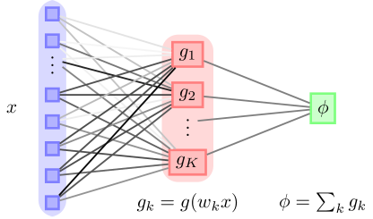
Figure 1: Neural network with a single hidden layer. A network with $K$ hidden units and weights $w$ implements a scalar function of its inputs $x$, $y=\sum_{k}^{K}g(w_{k}x)$, where $g:\mathbb{R}\to\mathbb{R}$ is the non-linear activation function of the network.

2.2 The student aims to mimic the teacher’s function

Once a teacher network has been chosen at random, we train another neural network, called the student, on data generated by the teacher according to (4). The student has a single fully-connected hidden layer with $K$ hidden units, and we explicitly allow for $K\neq M$. The student’s weights from the input to the hidden layer are denoted $w\in\mathbb{R}^{K\times N}$ and its output is given by $\phi(w,x)$. We keep the weights from the hidden units to the output fixed at unity and only train the first layer weights $w$. We consider both networks in the thermodynamic limit, where we let $N\to\infty$ while keeping $M,K$ of order 1.

The key quantity in our study is the generalisation error of the student network with respect to the teacher network, which we defined in Eq. (1) as the mean squared error between the outputs of the student and the noiseless output of the teacher, averaged over the distribution of inputs. Note that including the output noise of the teacher would only introduce a constant offset proportional to the variance of the output noise.

2.3 The student is trained using online learning

Since we are training the student for a regression task, we choose a quadratic loss function. Given a training data set with $P$ samples, the training error reads

$$E(w)=\frac{1}{2}\sum_{\mu=1}^{P}{\left(\phi(w,x^{\mu})-y_{B}^{\mu}\right)}^{2}.$$ (5)

We perform stochastic gradient descent on the training error to optimise the weights of the student, using only a single sample $(x^{\mu},y_{B}^{\mu})$ to evaluate the gradient of $E(w)$ at every step. To make the problem analytically tractable, we consider the limit where the training data set is large enough to allow that each sample $(x^{\mu}$, $y_{B}^{\mu})$ is visited only once during the entire training until the generalisation error converges to its final value. We can hence index the steps of the algorithm by $\mu$ and write the weight updates as

$$w_{k}^{\mu+1}=w_{k}^{\mu}-\frac{\kappa}{N}w_{k}^{\mu}-\frac{\eta}{\sqrt{N}}\nabla_{w_{k}}E(w)|_{(x^{\mu},y_{B}^{\mu})}$$ (6)

where $\kappa$ is the weight decay rate, the learning rate is $\eta$, and we have chosen their scaling with $N$ such that all terms remain of order 1 in the thermodynamic limit $N\to\infty$. Evaluating the derivative yields

$$w_{k}^{\mu+1}=w_{k}^{\mu}-\frac{\kappa}{N}w_{k}^{\mu}-\frac{\eta}{\sqrt{N}}x^{\mu}r_{k}^{\mu}$$ (7)

where

$$r_{k}^{\mu}\equiv g^{\prime}(\lambda_{k}^{\mu})\left[\phi(w,x^{\mu})-y_{B}^{\mu}\right]$$ (8)

and we have defined $\lambda_{k}^{\mu}\equiv w_{k}x^{\mu}/\sqrt{N}$.

Stochastic gradient descent with mini-batch size 1 in the limit of very large training sets is also known as online or one-shot learning. Kinzel [35] first realised that its dynamics could be described in terms of order parameters, initiating a number of works on the perceptron [36, 21]. Online learning in committee machines was first studied by Biehl and Schwarze [15] in the case $M=1,K=2$ and by Saad and Solla [17, 37], who gave a detailed analytic description of the case $K=M$ with $g(x)=\operatorname{erf}\left(x/\sqrt{2}\right)$. Beyond its application to neural networks, its performance has been analysed for problems ranging from PCA [38, 39] to the training of generative adversarial networks [40].

2.4 The dynamics of online learning can be described in closed form

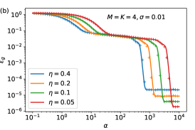
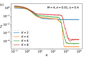
Figure 2: The analytical description of the generalisation dynamics of sigmoidal networks (solid) matches simulations (crosses). We show learning curves $\epsilon_{g}(\alpha)$ obtained by integration of the ODEs (12) (solid). From left to the right, we vary the variance of the teacher’s output noise $\sigma$, the learning rate $\eta$, and the number of hidden units in the student $K$. For each combination of parameters shown in the plots, we ran a single simulation of a network with $N=784$ and plot the generalisation observed (crosses). $\kappa=0$ in all cases.

Our aim is to track the evolution of the generalisation error $\epsilon_{g}$ (1), which can be written more explicitly as

$$\epsilon_{g}=\frac{1}{2}\left\langle{\left[\sum_{k=1}^{K}g\left(\lambda_{k}^{\mu}\right)-\sum_{m=1}^{M}g(\nu_{m}^{\mu})\right]}^{2}\right\rangle,$$ (9)

where $\nu_{m}^{\mu}\equiv B_{m}x^{\mu}/\sqrt{N}$. Since the inputs $x$ only appear as products with the weight vectors of the student and the teacher, we can replace the average $\langle\cdot\rangle$ over $x$ with an average over $\lambda_{k}^{\mu}$ and $\nu_{m}^{\mu}$. To determine the distribution of the latter, the assumption that every sample $(x^{\mu},y_{B}^{\mu})$ is only used once during training becomes crucial, because it guarantees that the inputs and the weights of the networks are uncorrelated. By the central limit theorem, $\nu_{m}^{\mu},\lambda_{k}^{\mu}$ are hence normally distributed with mean zero since $\langle x_{n}\rangle=0$. Their covariance is also easily found: writing $w_{ka}$ for a component of the $k$th weight vector, we have

$$\langle\lambda_{k}\lambda_{l}\rangle=\frac{\sum_{a,b}^{N}w_{ka}w_{lb}\langle x_{a}x_{b}\rangle}{N}=\frac{w_{k}w_{l}}{N}\equiv Q_{kl}$$ (10)

since $\langle x_{a}x_{b}\rangle=\delta_{ab}$. Likewise, we define

$$\langle\nu_{n}\nu_{m}\rangle=\frac{B_{n}B_{m}}{N}\equiv T_{nm},\quad\langle\lambda_{k}\nu_{m}\rangle=\frac{w_{k}B_{m}}{N}\equiv R_{km}.$$ (11)

The variables $R_{in}$, $Q_{ik}$, and $T_{nm}$ are called order parameters in statistical physics and measure the overlap between student and teacher weight vectors $w_{i}$ and $B_{n}$ and their self-overlaps, respectively. Crucially, from Eq. (9) we see that they are sufficient to determine the generalisation error $\epsilon_{g}$.

We can obtain a closed set of differential equations for the time evolution of the order parameters $Q$ and $R$ by squaring the weight update (7) and taking its inner product with $B_{n}$, respectively. Then, an average over the inputs $x$ needs to be taken. The resulting equations of motion for $R$ and $Q$ can be written as

$$\frac{\operatorname{d}\!R_{in}}{\operatorname{d}\!\alpha} =-\kappa R_{in}+\eta\langle r_{i}\nu_{n}\rangle$$ (12a)

$$\begin{split}\frac{\operatorname{d}\!Q_{ik}}{\operatorname{d}\!\alpha}&=-2\kappa Q_{ik}+\eta\langle r_{i}\lambda_{k}\rangle+\eta\langle r_{k}\lambda_{i}\rangle\\ &\qquad+\eta^{2}\langle r_{i}r_{k}\rangle+\eta^{2}\sigma^{2}\langle g^{\prime}(\lambda_{i})g^{\prime}(\lambda_{k})\rangle\end{split}$$ (12b)

where $\alpha=\mu/N$ becomes a continuous time-like variable in the limit $N\to\infty$. The averages over inputs $\langle\cdot\rangle$ can again be reduced to an average over the normally distributed local fields $\lambda_{k}^{\mu}$ and $\nu_{m}^{\mu}$ as above. If the averages can be evaluated analytically, the equations of motion (12) together with the generalisation error (9) form a closed set of equations which can be integrated numerically and provides an exact description of the generalisation dynamics of the network in the limit of large $N$ and large training sets. Indeed, the integrals have an analytical solution for the choice $g(x)=\operatorname{erf}(x/\sqrt{2})$ [15] and for linear networks. Eqns. (12) hold for any $M$ and $K$, enabling us to study the learning of complex non-linear target functions $\phi(B,x)$, rather than data that is linearly separable or follows a Gaussian distribution [41, 42]. A detailed derivation and the explicit form of the equations of motion are given in Appendix A.

We plot $\epsilon_{g}(\alpha)$ obtained by numerically integrating Eqns. (12) and the generalisation error observed during a single run of online learning (7) with $N=784$ in Fig. 2. The plots demonstrate a good quantitative agreement between simulations and theory and display some generic features of online learning in soft committee machines.

One notable feature of all the plots in Fig. 2 is the existence of plateaus during training, where the generalisation error is almost stationary. During this time, the student “believes” that data are linearly separable and all its hidden units have roughly the same overlap with all the hidden units of the teacher. Only after a longer time, the student picks up the additional structure of the teacher and “specialises”: each of its hidden units ideally becomes strongly correlated with one and only one hidden unit of the teacher before the generalisation error decreases exponentially to its final value. This effect is well-known in the literature for both batch and online learning [28, 15, 16] and will be revisited in Sec. 3.

It is perhaps surprising that the generalisation dynamics seem unaffected by the difference in output noise (Fig. 2 a) until they leave the plateau. This is due to the fact that the noise appears in the equations of motion only in terms that are quadratic in the learning rate. Their effect takes longer to build up and become significant. The specialisation observed above is also due to terms that are quadratic in the learning rate. This goes to show that even in the limit of small learning rates, one cannot simplify the dynamics of the neural network by linearising Eqns. (12) in $\eta$ without losing some key properties of the dynamics.

3 Asymptotic generalisation of over-parameterised students after online learning

In the absence of output noise ($\sigma=0$) and without weight decay ($\kappa=0$), online learning of a student with $K\geq M$ hidden units will yield a network that generalises perfectly with respect to the teacher. More precisely, at some point during training, the generalisation error will start an exponential decay towards zero (see Appendix B.1). On the level of the order parameters $Q$ and $R$, a student that generalises perfectly with respect to the teacher corresponds to a stable fixed point of the equations of motion (12) with $\epsilon_{g}=0$.

This fixed point disappears for $\sigma>0$ and the order parameters converge to a different fixed point. The values of the order parameters at that fixed point can be obtained perturbatively in the limit of small noise, i.e.  small $\sigma$. To this end, we first make an ansatz for the matrices $Q$ and $R$ that involves eight order parameters for any $M,K$. We choose this number of order parameters for two reasons: it is the smallest number of variables for which we were able to self-consistently close the equations of motion (12), and they agree with numerical evidence obtained from integrating the full equations of motion (12).

We then derive equations of motion for this reduced set of order parameters, and expand them to first order in $\sigma$ around the fixed point with perfect generalisation. Throughout this section, we set $\kappa=0$ and choose uncorrelated and isotropic weight vectors for the teacher, i.e. $T_{nm}=\delta_{nm}$, which is equivalent to drawing the weights at random from a standard normal distribution.

3.1 Sigmoidal networks

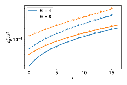
Figure 3: Theoretical predictions for $\epsilon_{g}^{*}$ match simulations. We plot theoretical predictions for $\epsilon_{g}^{*}/\sigma^{2}$ for sigmoidal networks (Eq. (13), solid line) and linear networks (Eq. (15), dashed) together with the result from a single simulation of a network with $N=784$. Parameters: $\eta=0.05,\sigma=0.01$.

We have performed this calculation for teacher and student networks with $g(x)=\operatorname{erf}(x/\sqrt{2})$. We discuss the details of this tedious calculation in Appendix 3, and here we only state the asymptotic value of the generalisation error $\epsilon_{g}^{*}$ to first order in the variance of the noise $\sigma^{2}$ for teacher and student with sigmoidal activation:

$$\epsilon_{g}^{*}=\frac{\sigma^{2}\eta}{2\pi}f(M,L,\eta)+\mathcal{O}(\sigma^{3})$$ (13)

where $f(M,L,\eta)$ is a lengthy rational function of its variables. The full expression spans more than two pages, so here we plot it in Fig. 3 together with a single run of a simulation of a neural network with $N=784$, which is in excellent agreement.

3.1.1 Discussion

One notable feature of Fig. 3 is that with all else being equal, the generalisation error increases monotonically with $L$. In other words, our result (13) implies that SGD alone fails to regularise the student networks of increasing size in our setup, instead yielding students whose generalisation error increases at least linearly with $L$.

One might be tempted to mitigate this effect by simultaneously decreasing the learning rate $\eta$ for larger students. However, this raises two problems: first of all, a lower learning rate means the model would take longer to train. More importantly though, the resulting longer training time implies that more data is required until the final generalisation error is achieved. This is in agreement with statistical learning theory, where given more and more data, models with more parameters (higher $L$) and a higher complexity class, e.g. a higher VC dimension or Rademacher complexity [6], generalise just as well as smaller ones. In practice however, more data might not be readily available. Furthermore, we show in the Appendix B.2.1 that even when we choose $\eta=1/K$, the generalisation error still increases with $L$ before plateauing at a constant value.

We can gain some intuition for the result (13) by considering the final representations learnt by a sigmoidal network. On the left half of Fig. 4, we plot the overlap matrices $Q$ and $R$ for a teacher with $M=2$ and various $K$. For $K=2$, we see that each of the hidden units of the student has learnt the weights of one teacher hidden unit, yielding diagonal matrices $Q$ and $R$ (modulo the permutation symmetry of the hidden units). As we add a third hidden unit to the student, $K=3$, the specialisation discussed in the previous section becomes apparent: two of the hidden units of the student each align almost perfectly with a different hidden unit of the teacher, such that $R_{01}=R_{20}\approx 1$, while the weights of the third unit go to zero ($Q_{11}\approx 0$). As we add even more hidden units, ($K=5$), the weight vectors of some units become exactly anti-correlated, hence effectively setting their weights to zero as far as the output of that network is concerned (since we set the weights of the second layer to unity). This behaviour is essentially a consequence of the sigmoidal form of the activation function, which makes it hard to express the sum of $M$ hidden units with $K\neq M$ hidden units, instead forcing 1-to-1 specialisation of the student’s hidden units.

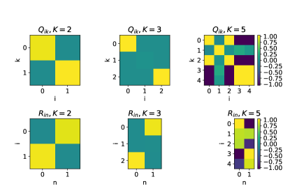
Figure 4: Sigmoidal networks learn different representations from a noisy teacher than ReLU networks. For sigmoidal networks (left), we see clear signs of specialisation as described in Sec. 3.1: for $K=3$, one unit is simply shut down: $w_{1}=0$. As we increase $K$, some units become exactly anti-correlated to each other (e.g. units 1, 4 for $K=5$), hence effectively setting their weights to zero (we keep the weights of the second layer fixed at unity). ReLU networks instead find representations where several nodes are used. Parameters: $N=784,\eta=0.3,\sigma=0.1,\kappa=0$.

In the over-parameterised case, $L=K-M$ units of the student are hence effectively specialising to hidden units of the teacher with zero weights. Although their weights are unbiased estimators of the weights $B=0$, their variance is finite due to the noise in the teacher’s output. Thus they always hurt generalisation.

This intuition can be confirmed analytically by going to the limit of small learning rates, which is the most relevant in practice. Expanding $\epsilon_{g}^{*}$ to first order in the learning rate reveals a particularly revealing form,

$$\epsilon_{g}^{*}=\frac{\sigma^{2}\eta}{2\pi}\left(L+\frac{M}{\sqrt{3}}\right)+\mathcal{O}(\eta^{2}),$$ (14)

with second-order corrections that are quadratic in $L$. The linear term in $\eta$ is the sum of two contributions: the asymptotic generalisation errors of $M$ independent networks with one hidden units that are learning from a teacher with single hidden unit hand $T=1$. The $L=K-M$ superfluous units contribute each the error of a continuous perceptrons that is learning from a teacher with zero weights ($T=0$). Again, we relegate the detailed calculation to the Appendix C.

3.2 Linear networks

One might suspect that part of the scaling $\epsilon_{g}^{*}\sim L$ in sigmoidal networks is due to the specialisation of the hidden units or the fact that teacher and student network can implement functions of different range if $K\neq M$. It thus makes sense to calculate $\epsilon_{g}^{*}$ for linear neural networks, where $g(x)=x$ [43]. These networks have no specialisation transition [26] and their output range is set by the magnitude of their weights, rather than their number of hidden units. Furthermore, linear networks are receiving increasing attention as models for neural networks [44, 25, 45].

Following the same steps as for the sigmoidal networks, a perturbative calculation in the limit of small noise yields

$$\epsilon_{g}^{*}=\frac{\eta\sigma^{2}(L+M)}{4-2\eta(L+M)}+\mathcal{O}(\sigma^{3}).$$ (15)

In the limit of small learning rates, the above expression further simplifies to

$$\epsilon_{g}^{*}=\frac{1}{4}\eta\sigma^{2}(L+M)+\mathcal{O}\left(\eta^{2}\right).$$ (16)

Hence we see that in the limit of small learning rates, the asymptotic generalisation error of linear networks has the same scaling with $\sigma$, $\eta$ and $L$ as for sigmoidal networks. This result is again in good agreement with the results of simulations, demonstrated in Fig. 3.

3.2.1 Discussion

The linear scaling of $\epsilon_{g}^{*}$ with $L$, keeping all other things equal, might be surprising given that all linear networks implement a linear transformation with an effective matrix $W=\sum_{k}w_{k}$, irrespective of their number of hidden units. However, this is exactly the problem: adding hidden units to a linear network does not augment the class of functions it can implement, but it adds free parameters which will indiscriminately pick up fluctuations due to the output noise in the teacher. The optimal generalisation error is indeed realised with $K=1$ irrespective of $M$, since a linear network with $K=1$ has the lowest number of free parameters while having the same expressive power as a teacher with arbitrary $M$. Our formula (15) however only applies to the case $K>M$.

Linear networks thus show that the scaling of $\epsilon_{g}^{*}$ with $L$ is not only a consequence of either specialisation or the mismatched range of the networks’ output functions, as one might have suspected by looking only at sigmoidal networks.

Interestingly, if we rescale the learning rate by choosing $\eta=1/K$, we find that the generalisation error (15) becomes equal to $\sigma^{2}/2$, independent of $L$. Again, this rescaling of the learning rate comes at the cost of increased training time and hence, in this model, increased training data. A quantitative exploration of the trade-off between learning rate and network size for a fixed data set is an interesting problem, however, it goes beyond the domain of online learning and is hence left for future work.

3.3 Numerical results suggest the same scalings for ReLU networks, too

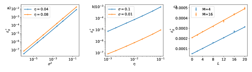
Figure 5: The final generalisation error of over-parametrised ReLU networks scales as $\epsilon_{g}^{*}\sim\eta\sigma^{2}L$. Simulations confirm that the asymptotic generalisation error $\epsilon_{g}^{*}$ of a ReLU student learning from a ReLU teacher scales with the learning rate $\eta$, the variance of the teacher’s output noise $\sigma^{2}$ and the number of additional hidden units as $\epsilon_{g}\sim\eta\sigma^{2}L$, which is the same scaling as the one found analytically for sigmoidal networks in Eq. (14). Straight lines are linear fits to the data, with slope $1$ in (a) and (b). Parameters: $M=2,K=6$ (a, b) and $M=4,16$; $K=M+L$ (c); in all figures, $N=784,\kappa=0$.

The analytical calculation of $\epsilon_{g}$ described above for networks with ReLU activation function poses some additional technical challenges, so here we resort to simulations to illustrate the behaviour of $\epsilon_{g}^{*}$ in this case and leave the analytical description for future work. The results are shown in Fig. 5: we found numerically that the asymptotic generalisation error of a ReLU student learning from a ReLU teacher has the same scaling as the one we found analytically for networks with sigmoidal and with linear activation functions: $\epsilon_{g}^{*}\sim\eta\sigma^{2}L$.

3.3.1 Discussion

Looking at the final overlap matrices $Q$ and $R$ for ReLU networks in the right half of Fig. 4, we see a mechanism behind Eq. (2) for ReLU networks that is reminiscent of the linear case: instead of the one-to-one specialisation of sigmoidal networks, all the hidden units of the student have a finite overlap with all the hidden units of the teacher. This is a consequence of the fact that it is much simpler to re-express the sum of $M$ ReLU units with $K\neq M$ ReLU units. However, this also means that there are a lot of redundant degrees of freedom, which nevertheless all pick up fluctuations from the output noise and degrade the generalisation error.

For ReLU networks, one might imagine that several ReLU units can specialise to one and only one teacher unit and thus act as an effective denoiser for that teacher unit. However, we have checked numerically that this configuration is not a stable fixed point of the SGD dynamics.

4 Discussion

The main result of the preceding section was a set of ODEs that described the generalisation dynamics of over-parameterised two-layer neural networks. This framework allowed us to derive the scaling of the generalisation error of the student with the network size, the learning rate and the noise level in the teacher’s outputs. This scaling is robust with respect to the choice of the activation function as it holds true for linear, sigmoidal and ReLU networks. In this section, we discuss several possible changes to our setup and discuss their impact on the scaling of $\epsilon_{g}^{*}$.

4.1 Weight decay

A natural strategy to avoid overfitting is to explicitly regularise the weights, for example by using weight decay. In our setup, this is introduced by choosing a finite $\kappa>0$ in Eq. (7). In our simulations with $\kappa>0$, we did not find a scenario where weight decay did not increase the final generalisation error compared to the case $\kappa=0$. In particular, we did not find a scenario where weight decay improved the performance of a student with $L>0$. The corresponding plots can be found in Appendix D.

4.2 SGD with mini-batches

We also made sure that the phenomenology we observed persists if we move to stochastic gradient descent with mini-batches, where the gradient estimate in Eq. (7) is averaged over several samples $(x,y_{B})$, as is standard in practice. We observed that increasing the mini-batch size lowers the asymptotic generalisation error up to a certain mini-batch size of order $\sim 100$ samples, after which it stays roughly constant. Crucially, having mini-batches does not change the scaling of $\epsilon_{g}^{*}$ with $L$ (see Appendix E for details).

4.3 Structured input data

One idealised assumption in our setup is that we take our inputs $x$ as i.i.d. draws from a standard normal distribution (see Sec. 2). We therefore repeated our experiments using MNIST images as inputs $x$, while leaving all other aspects of our setup the same. In particular, we still trained the student on a regression task with $y$ generated using a random teacher. This setup allowed us to trace any change in the generalisation behaviour of the student to the higher-order correlations of the input distribution. Switching to MNIST inputs reproduced the same $\epsilon_{g}$-$L$ curve as having Gaussian inputs to within the experimental error; the interested reader is referred to Appendix F for a detailed description of these experiments.

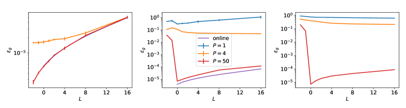
Figure 6: The scaling of $\epsilon_{g}^{*}$ with $L$ depends on the size of the training set. We plot $\epsilon_{g}^{*}$ after SGD with a finite training set with $PN$ samples for linear, sigmoidal and ReLU networks from left to right. The result for online learning for linear and sigmoidal networks, Eqns. (13) and (15), are plotted in violet. In the linear case, the online learning result exactly matches the simulation for $P=50$. Error bars indicate one standard deviation over 10 simulations, each with a different training set; many of them are too small to be clearly visible. Parameters: $N=784,M=4,\eta=0.1,\sigma=0.01$.

4.4 The scaling of $\epsilon_{g}^{*}$ with $L$ depends also on the size of the training set

In practice, a single sample of the training data set will be visited several times during training. After a first pass through the training set, the online assumption that an incoming sample $(x,y_{B})$ is uncorrelated to the weights of the network thus breaks down. A complete analytical treatment in this setting remains an open problem, so to study this practically relevant setup, we turn to simulations. We keep the setup described in Sec. 2, but simply reduce the number of samples in the training data set $P$. Our focus is again on the final generalisation error after convergence $\epsilon_{g}^{*}$ for linear, sigmoidal and ReLU networks, which we plot from left to right as a function of $L$ in Fig. 6.

Linear networks show a similar behaviour to the setup with a very large training set discussed in Sec. 3.2: the bigger the network, the worse the performance for both $P=4$ and $P=50$. Again, the optimal network has $K=1$ hidden units, irrespective of the size of the teacher. However, for non-linear networks, the picture is more varied: For large training sets, where the number of samples easily outnumber the free parameters in the network ($P=50$, red curve; this corresponds roughly to learning a data set of the size of MNIST), the behaviour is qualitatively described by our theory from Sec. 3: the best generalisation is obtained by a network that matches the teacher size, $K=M$. However, as we reduce the size of the training set, this is no longer true. For $P=4$, for example, the best generalisation is obtained with networks that have $K>M$. Thus the size of the training set with respect to the network has an important influence on the scaling of $\epsilon_{g}^{*}$ with $L$. Note that the early-stopping generalisation error, which we define as the minimal generalisation error over the duration of training, shows qualitatively the same behaviour as $\epsilon_{g}^{*}$ (see Appendix G for additional information.)

5 Concluding perspectives

We have studied the dynamics of online learning in two-layer neural networks within the teacher-student framework, where we train a student network using SGD on data generated by another network, the teacher. One advantage of this setup is that it allows us to investigate the behaviour of networks that are over-parameterised with respect to the generative model of their data in a controlled fashion. We derived a set of eight ODEs that describe the generalisation dynamics of over-parameterised students of any size. Within this framework, we analytically computed the final generalisation error of the student in the limit of online learning with small noise. One immediate consequence of this result is that SGD alone is not enough to regularise the over-parameterised student, instead yielding networks whose generalisation error scales linearly with the network size.

Furthermore, we demonstrated that adding explicit regularisation by introducing weight decay did not improve the performance of the networks and that the same phenomenology arises when using mini-batches or after substituting the Gaussian inputs used in the theoretical analysis with a more realistic data set. Nevertheless, we were able to find a scenario in our setup where the generalisation decreases with the student’s size, namely when training using a finite data set that contains roughly as many samples as there are free parameters in the network.

In the setting we analyse, our results clearly indicate that the regularisation of neural networks goes beyond the properties of SGD alone. Instead, a full understanding of the generalisation properties of deep networks requires taking into account the interplay of at least the algorithm, its learning rate, the model architecture, and the data set, setting up a formidable research programme for the future.

Appendix A Derivation of the ODE description of the generalisation dynamics of online learning

We will now show how to derive ODEs that describe the dynamics of online learning in two-layer neural networks, following the seminal work by Biehl and Schwarze [15] and Saad and Solla [16, 17]. We focus on the teacher-student setup introduced in the main paper, where a student network with weights $w\in\mathbb{R}^{K\times N}$ and output

$$\phi(w,x)=\sum_{k=1}^{K}g\left(\frac{w_{k}x}{\sqrt{N}}\right)$$ (17)

is trained on samples $(x^{\mu},y^{\mu})$ generated by another two-layer network with weights $B\in\mathbb{R}^{M\times N}$, the teacher, according to

$$y^{\mu}_{B}(x^{\mu})\equiv\phi(B,x^{\mu})+\zeta^{\mu}.$$ (18)

Here, $\zeta^{\mu}$ is normally distributed with mean $0$ and variance $\sigma^{2}$. We will make two technical assumptions, namely having a large network ($N\to\infty$) and a data set that is large enough to allow that we visit every sample only once before training converges.

A.1 Expressing the generalisation error in terms of order parameters

To make this section self-consistent, we briefly recapitulate how the assumptions stated above allow to rewrite the generalisation error in terms of a number of order parameters. We have

$$\epsilon_{g}\equiv \frac{1}{2}\left\langle{\left[\phi(w,x)-\phi(B,x)\right]}^{2}\right\rangle$$ (19)

$$= \frac{1}{2}\left\langle{\left[\sum_{k=1}^{K}g\left(\lambda_{k}^{\mu}\right)-\sum_{m=1}^{M}g(\nu_{m}^{\mu})\right]}^{2}\right\rangle,$$ (20)

where we have introduced the local fields

$$\lambda_{k}^{\mu}\equiv \frac{w_{k}x^{\mu}}{\sqrt{N}},$$ (21)

$$\nu_{m}^{\mu}\equiv \frac{B_{m}x^{\mu}}{\sqrt{N}}.$$ (22)

Here and throughout this paper, we will use the indices $i,j,k,\ldots$ to refer to hidden units of the student, and indices $n,m,\ldots$ to denote hidden units of the teacher. Since the input $x^{\mu}$ only appears in $\epsilon_{g}$ only via products with the weights of the teacher and the student, we can replace the high-dimensional average $\langle\cdot\rangle$ over the input distribution $p(x)$ by an average over the $K+M$ local fields $\lambda_{k}^{\mu}$ and $\nu_{m}^{\mu}$. The assumption that the training set is large enough to allow that we visit every sample in the training set only once guarantees that the inputs and the weights of the networks are uncorrelated. Taking the limit $N\to\infty$ ensures that the local fields are jointly normally distributed with mean zero ($\langle x_{n}\rangle=0$). Their covariance is also easily found: writing $w_{ka}$ for the $a$th component of the $k$th weight vector, we have

$$\langle\lambda_{k}\lambda_{l}\rangle=\frac{\sum_{a,b}^{N}w_{ka}w_{lb}\langle x_{a}x_{b}\rangle}{N}=\frac{w_{k}w_{l}}{N}\equiv Q_{kl},$$ (23)

since $\langle x_{a}x_{b}\rangle=\delta_{ab}$. Likewise, we define

$$\langle\nu_{n}\nu_{m}\rangle=\frac{B_{n}B_{m}}{N}\equiv T_{nm},\quad\langle\lambda_{k}\nu_{m}\rangle=\frac{w_{k}B_{m}}{N}\equiv R_{km}.$$ (24)

The variables $R_{in}$, $Q_{ik}$, and $T_{nm}$ are called order parameters in statistical physics and measure the overlap between student and teacher weight vectors $w_{i}$ and $B_{n}$ and their self-overlaps, respectively. Crucially, from Eq. (20) we see that they are sufficient to determine the generalisation error $\epsilon_{g}$. We can thus write the generalisation error as

$$\epsilon_{g}=\frac{1}{2}\sum_{i,k}I_{2}(i,k)+\frac{1}{2}\sum_{n,m}I_{2}(n,m)-\sum_{i,n}I_{2}(i,n),$$ (25)

where we have defined

$$I_{2}(i,k)\equiv\langle g(\lambda_{i})g(\lambda_{k})\rangle=\frac{1}{\pi}\arcsin\frac{Q_{ik}}{\sqrt{1+Q_{ii}}\sqrt{1+Q_{kk}}}.$$ (26)

The average in Eq. (26) is taken over a normal distribution for the local fields $\lambda_{i}$ and $\lambda_{k}$ with mean $(0,0)$ and covariance matrix

$$C_{2}=\begin{pmatrix}Q_{ii}&Q_{ik}\\ Q_{ik}&Q_{kk}\end{pmatrix}.$$ (27)

Since we are using the indices $i,j,\ldots$ for student units and $n,m,\ldots$ for teacher hidden units, we have

$$I_{2}(i,n)=\langle g(\lambda_{i})g(\nu_{m})\rangle,$$ (28)

where the covariance matrix of the joint of distribution $\lambda_{i}$ and $\nu_{m}$ is given by

$$C_{2}=\begin{pmatrix}Q_{ii}&R_{in}\\ T_{in}&T_{nn}\end{pmatrix}.$$ (29)

and likewise for $I_{2}(n,m)$. We will use this convention to denote integrals throughout this section. For the generalisation error, this means that it can be expressed in terms of the order parameters alone as

$$\epsilon_{g}=\frac{1}{\pi}\sum_{i,k}\arcsin\frac{Q_{ik}}{\sqrt{1+Q_{ii}}\sqrt{1+Q_{kk}}}+\frac{1}{\pi}\sum_{n,m}\arcsin\frac{T_{nm}}{\sqrt{1+T_{nn}}\sqrt{1+T_{mm}}}\\ -\frac{2}{\pi}\sum_{i,n}\arcsin\frac{R_{in}}{\sqrt{1+Q_{ii}}\sqrt{1+T_{nn}}}.$$ (30)

A.2 ODEs for the evolution of the order parameters

Expressing the generalisation error in terms of the order parameters as we have in Eq. (30) is of course only useful if we can track the evolution of the order parameters over time. We can derive ODEs that allow us to do precisely that by first writing again the SGD update of the weights:

$$w_{k}^{\mu+1}=w_{k}^{\mu}-\frac{\kappa}{N}w_{k}^{\mu}-\frac{\eta}{\sqrt{N}}x^{\mu}r_{k}^{\mu},$$ (31)

where $\mu$ is a running index counting the weight updates or, equivalently, the samples used so far, and

$$r_{k}^{\mu}\equiv g^{\prime}(\lambda_{k}^{\mu})\left[\phi(w,x^{\mu})-y_{B}^{\mu}\right].$$ (32)

From this equation, we can obtain differential equations for the time evolution of the order parameters $Q$ by squaring the weight update (31) and for $R$ taking the inner product of (31) with $B_{n}$, respectively, which yields the Eqns. (12) of the main text and which we state again for completeness:

$$\frac{\operatorname{d}\!R_{in}}{\operatorname{d}\!\alpha} =-\kappa R_{in}+\eta\langle r_{i}\nu_{n}\rangle$$ (33a)

$$\frac{\operatorname{d}\!Q_{ik}}{\operatorname{d}\!\alpha} =-2\kappa Q_{ik}+\eta\langle r_{i}\lambda_{k}\rangle+\eta\langle r_{k}\lambda_{i}\rangle+\eta^{2}\langle r_{i}r_{k}\rangle+\eta^{2}\sigma^{2}\langle g^{\prime}(\lambda_{i})g^{\prime}(\lambda_{k})\rangle$$ (33b)

where $\alpha=\mu/N$ becomes a continuous time-like variable in the limit $N\to\infty$. These equations are valid for any choice of activation functions $g_{1}$ and $g_{2}$. To make progress however, i.e. to obtain a closed set of differential equations for $Q$ and $R$, we need to evaluate the averages $\langle\cdot\rangle$ over the local fields. In particular, we have to compute three types of averages:

$$I_{3}=\langle g^{\prime}(a)bg^{\prime}(c)\rangle,$$ (34)

where $a$ is one the local fields of the student, while $b$ and $c$ can be local fields of either the student or the teacher;

$$I_{4}=\langle g^{\prime}(a)g^{\prime}(b)g(c)g(d)\rangle,$$ (35)

where $a$ and $b$ are local fields of the student, while $c$ and $d$ can be local fields of both; and finally

$$J_{2}=\langle g^{\prime}(a)g^{\prime}(b)\rangle,$$ (36)

where $a$ and $b$ are local fields of the teacher. In each of these integrals, the average is taken with respect to a multivariate normal distribution for the local fields with zero mean and a covariance matrix whose entries are chosen in the same way as discussed for $I_{2}$.

We can re-write Eqns. (33) with these definitions in a more explicit form as [16, 17]

$$\frac{\operatorname{d}\!R_{in}}{\operatorname{d}\!\alpha} =-\kappa R_{in}+\eta\left(\sum_{m}I_{3}(i,n,m)-\sum_{j}I_{3}(i,n,j)\right),$$ (37)

$$\frac{\operatorname{d}\!Q_{ik}}{\operatorname{d}\!\alpha} =-2\kappa Q_{ik}+\eta^{2}\sigma^{2}J_{2}(i,k)$$

$$\quad+\eta\left(\sum_{m}I_{3}(i,k,m)-\sum_{j}I_{3}(i,k,j)\right)$$

$$\quad+\eta\left(\sum_{m}I_{3}(k,i,m)-\sum_{j}I_{3}(k,i,j)\right)$$

$$\quad+\eta^{2}\left(\sum_{n,m}I_{4}(i,k,n,m)-2\sum_{j,n}I_{4}(i,k,j,n)+\sum_{j,l}I_{4}(i,k,j,l)\right).$$ (38)

The explicit form of the integrals $I_{2}(\cdot)$, $I_{3}(\cdot)$, $I_{4}(\cdot)$ and $J_{2}(\cdot)$ is given in Sec. H for the case $g(x)=\operatorname{erf}\left(x/\sqrt{2}\right)$. Solving these equations numerically for $Q$ and $R$ and substituting their values in to the expression for the generalisation error (25) gives the full generalisation dynamics of the student. We show the resulting learning curves together with the result of a single simulation in Fig. 2 of the main text. We have bundled our simulation software and our ODE integrator as a user-friendly Python package. In Sec. B, we discuss how to extract information from them in an analytical way.

Appendix B Calculation of $\epsilon_{g}$ in the limit of small noise

Our aim is to understand the asymptotic value of the generalisation error

$$\epsilon_{g}^{*}\equiv\lim_{\alpha\to\infty}\epsilon_{g}(\alpha).$$ (39)

We focus on students that have more hidden units than the teacher, $K\geq M$. These students are thus over-parameterised with respect to the generative model of the data and we define

$$L\equiv K-M$$ (40)

as the number of additional hidden units in the student network. In this section, we focus on the sigmoidal activation function

$$g(x)=\operatorname{erf}\left(x/\sqrt{2}\right),$$ (41)

unless stated otherwise.

Eqns. (37) are a useful tool to analyse the generalisation dynamics and they allowed Saad and Solla to gain plenty of analytical insight into the special case $K=M$ [16, 17]. However, they are also a bit unwieldy. In particular, the number of ODEs that we need to solve grows with $K$ and $M$ as $K^{2}+KM$. To gain some analytical insight, we make use of the symmetries in the problem, e.g. the permutation symmetry of the hidden units of the student, and re-parametrised the matrices $Q_{ik}$ and $R_{in}$ in terms of eight order parameters that obey a set of self-consistent ODEs for any $K>M$. We choose the following parameterisation with eight order parameters:

$$Q_{ij}= \begin{cases}Q&\quad i=j\leq M,\\ C&\quad i\neq j;\;i,j\leq M,\\ D&\quad i>M,j\leq M\quad\mathrm{or}\quad i\leq M,j>M,\\ E&\quad i=j>M,\\ F&\quad i\neq j;\;i,j>M,\end{cases}$$ (42)

$$R_{in}= \begin{cases}R&\quad i=n,\\ S&\quad i\neq n;\;i\leq M,\\ U&\quad i>M,\end{cases}$$ (43)

which in matrix form for the case $M=3$ and $K=5$ read:

$$R=\begin{pmatrix}R&S&S\\ S&R&S\\ S&S&R\\ U&U&U\\ U&U&U\end{pmatrix}\quad\mathrm{and}\quad Q=\begin{pmatrix}Q&C&C&D&D\\ C&Q&C&D&D\\ C&C&Q&D&D\\ D&D&D&E&F\\ D&D&D&F&E\\ \end{pmatrix}$$ (44)

We choose this number of order parameters and this particular setup for the overlap matrices $Q$ and $R$ for two reasons: it is the smallest number of variables for which we were able to self-consistently close the equations of motion (37), and they agree with numerical evidence obtained from integrating the full equations of motion (37).

By substituting this ansatz into the equations of motion (37), we find a set of eight ODEs for the order parameters. These equations are rather unwieldy and some of them do not even fit on one page, which is why we do not print them here in full; instead, we provide a Mathematica notebook where they can be found and interacted with. These equations allow for a detailed analysis of the effect of over-parameterisation on the asymptotic performance of the student, as we will discuss now.

B.1 Heavily over-parameterised students can learn perfectly from a noiseless teacher using online learning

For a teacher with $T_{nm}=\delta_{nm}$ and in the absence of noise in the teacher’s outputs ($\sigma=0$), there exists a fixed point of the ODEs with $R=Q=1$, $C=D=E=F=0$, and perfect generalisation $\epsilon_{g}=0$. Online learning will find this fixed point, as is demonstrated in Fig. 7, where we plot the generalisation dynamics of a student with $K$ hidden units learning from a teacher with $M=4$ hidden units for both Erf and ReLU activation functions. More precisely, after a plateau whose length depends on the size of the network for the sigmoidal network, the generalisation error eventually begins an exponential decay to the optimal solution with zero generalisation error. The learning rates are chosen such that learning converges, but aren’t optimised otherwise.

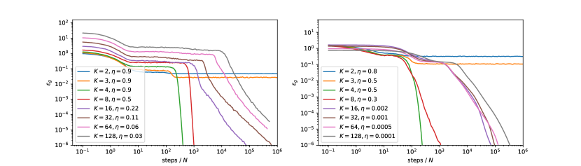
Figure 7: Over-parametrised networks with sigmoidal or ReLU activations learn perfectly from a noiseless teacher. The generalisation dynamics for students with sigmoidal (left) and ReLU activation function (right) for various $K$ learning from a teacher with $M=4$ is shown. In all cases, the generalisation error eventually decays exponentially towards zero. ($N=784$)

B.2 Perturbative solution of the ODEs

We have calculated the asymptotic value of the generalisation error $\epsilon_{g}^{*}$ for a teacher with $T_{nm}=\delta_{nm}$ to first order in the variance of the noise $\sigma^{2}$. To do so, we performed a perturbative expansion around the fixed point

$$R_{0}=Q_{0}=1,$$ (45)

$$S_{0}=U_{0}=C_{0}=D_{0}=E_{0}=F_{0}=0,$$ (46)

with the ansatz

$$X=X_{0}+\sigma^{2}X_{1}$$ (47)

for all the order parameters. Writing the ODEs to first order $\sigma^{2}$ and solving for their steady state where $X^{\prime}(\alpha)=0$ yielded a fixed point with an asymptotic generalisation error

$$\epsilon_{g}^{*}=\frac{\sigma^{2}\eta}{2\pi}f(M,L,\eta)+\mathcal{O}(\sigma^{3}).$$ (48)

$f(M,L,\eta)$ is an unwieldy rational function of its variables. Due to its length, we do not print it here in full; instead, we give the full function in a Mathematica notebook. Here, we plot the results in various forms in Fig. 8. We note in particular the following points:

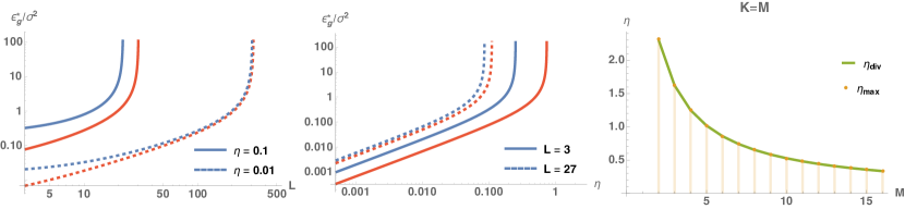
Figure 8: The final generalisation error of over-parameterised Erf networks scales linearly with the learning rate, the variance of the teacher’s output noise, and $L$. We plot $\epsilon_{g}^{*}/\sigma^{2}$ in the limit of small noise, Eq. (48), for $M=2$ (red) and $M=16$ (blue). It is clear that generalisation error increases with the number of superfluous units $L$ at fixed learning rate (left) and the learning rate $\eta$ (middle). Right: For $K=M$, the learning rate $\eta_{\mathrm{div}}$ at which our perturbative result diverges is precisely the maximum learning rate $\eta_{\max}$ at which the exponential convergence to the optimal solution is guaranteed for $\sigma=0$, Eq. (49)

B.2.1 Discussion

$\epsilon_{g}^{*}$ increases with $L$, $\eta$

The two plots on the left show that the generalisation error increases monotonically with both $L$ and $\eta$ while keeping the other fixed, resp., for teachers with $M=2$ (red) and $M=16$ (blue)

Divergence at large $\eta$

Our perturbative result diverges for large $L$, or equivalently, for a large learning rate that depends on the number of hidden units $L\sim K$. For the special case $K=M$, the learning rate $\eta_{\mathrm{div}}$ at which our perturbative result diverges is precisely the maximum learning rate $\eta_{\mathrm{max}}$ for which the exponential convergence to the optimal solution is still guaranteed for $\sigma=0$ [17]

$$\eta_{\max}=\frac{\sqrt{3}\pi}{M+3/\sqrt{5}-1}$$ (49)

as we show in the right-most plot of Fig. 8.

Expansion for small $\eta$

In the limit of small learning rates, which is the most relevant in practice and which from the plots in Fig. 8 dominates the behaviour of $\epsilon_{g}^{*}$ outside of the divergence, the generalisation error is linear in the learning rate. Expanding $\epsilon_{g}^{*}$ to first order in the learning rate reveals a particularly revealing form,

$$\epsilon_{g}^{*}=\frac{\sigma^{2}\eta}{2\pi}\left(L+\frac{M}{\sqrt{3}}\right)+\mathcal{O}(\eta^{2})$$ (50)

with second-order corrections that are quadratic in $L$. This is actually the sum of the asymptotic generalisation errors of $M$ continuous perceptrons that are learning from a teacher with $T=1$ and $L$ continuous perceptrons with $T=0$ as we calculate in Sec. C. This neat result is a consequence of the specialisation that is typical of SCMs with sigmoidal activation functions as we discussed in the main text.

Rescaling the learning rate by $K$

The expression for the generalisation error in the limit of small learning rates might tempt one to rescale the learning rate $\eta$ by $K$ in order to mitigate the detrimental effect of the over-parameterisation. As we note in the main text, this a leads to a longer training duration which in our model implies that more data is required until the final generalisation error is achieved, both of which might not be feasible in practice. Moreover, we show in Fig. 9 that the asymptotic generalisation error (48) of a student trained using SGD with learning rate $\eta=1/K$ still increases with $L$ before plateauing at a constant value that is independent of $M$.

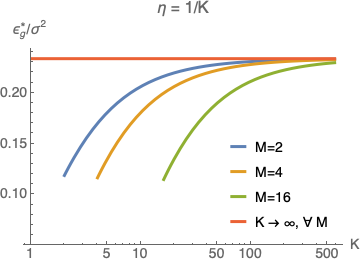
Figure 9: Asymptotic generalisation error for sigmoidal networks with learning rate $\eta=1/K$. We plot the asymptotic generalisation error $\epsilon_{g}^{*}$ (48) over $\sigma^{2}$ of a student with a varying number of hidden units trained on data generated by teachers with $M=2,4,16$ using SGD with learning rate $1/K$. The generalisation error still increases with $K$, before plateauing at a constant value that is independent of $M$. $\kappa=0$.

Appendix C Asymptotic generalisation error of a noisy continuous perceptron

What is the asymptotic generalisation for a continuous perceptron, i.e. a network with $K=1$, in a teacher-student scenario when the teacher has some additive Gaussian output noise? In this section, we repeat a calculation by Biehl and Schwarze [15] where the teacher’s outputs are given by

$$y_{B}=g\left(\frac{Bx}{\sqrt{N}}\right)+\zeta$$ (51)

where $\zeta$ is again a Gaussian random variable with mean 0 and variance $\sigma^{2}$. We keep denoting the weights of the student by $w$ and the weights of the teacher by $B$. To analyse the generalisation dynamics, we introduce the order parameters

$$R\equiv\frac{wB}{N},\qquad Q\equiv\frac{ww}{N}\quad\mathrm{and}\quad T\equiv\frac{BB}{N}.$$ (52)

and we explicitly do not fix $T$ for the moment. For $g(x)=\mathrm{erf}\left(x/\sqrt{2}\right)$, they obey the following equations of motion:

$$\frac{dR}{dt}= \frac{2\eta}{\pi\left(Q(t)+1\right)}\left(\frac{TQ(t)-R(t)^{2}+T}{\sqrt{(T+1)Q(t)-R(t)^{2}+T+1}}-\frac{R(t)}{\sqrt{2Q(t)+1}}\right)$$ (53)

$$\frac{dQ}{dt}= \frac{4\eta}{\pi(Q(t)+1)}\left(\frac{R(t)}{\sqrt{2(Q(t)+1)-R(t)^{2}}}-\frac{Q(t)}{\sqrt{2Q(t)+1}}\right)$$

$$+\frac{4\eta^{2}}{\pi^{2}\sqrt{2Q(t)+1}}\left[-2\arcsin\left(\frac{R(t)}{\sqrt{(6Q(t)+2)(2Q(t)-R(t)^{2}+1)}}\right)\right.$$

$$\qquad+\left.\arcsin\left(\frac{2\left(Q(t)-R(t)^{2}\right)+1}{2\left(2Q(t)-R(t)^{2}+1\right)}\right)+\arcsin\left(\frac{Q(t)}{3Q(t)+1}\right)\right]$$

$$+\frac{2\eta^{2}\sigma^{2}}{\pi\sqrt{2Q(t)+1}}.$$ (54)

The equations of motion have a fixed point at $Q=R=T$ which has perfect generalisation for $\sigma=0$. We hence make a perturbative ansatz in $\sigma^{2}$

$$Q(t)= T+\sigma^{2}q(t)$$ (55)

$$R(t)= T+\sigma^{2}r(t)$$ (56)

and find for the asymptotic generalisation error

$$\epsilon_{g}^{*}=\frac{\eta\sigma^{2}(4T+1)}{2\sqrt{2T+1}\left(-\eta\sqrt{8T^{2}+6T+1}+4\pi T+\pi\right)}+\mathcal{O}\left(\sigma^{3}\right).$$ (57)

To first order in the learning rate, this reads

$$\epsilon_{g}^{*}=\frac{\eta\sigma^{2}}{2\pi\sqrt{2T+1}},$$ (58)

which should be compared to the corresponding result for the full SCMs, Eq. (50).

Appendix D Regularisation by weight decay does not help

Figure 10: Weight decay. We plot the final generalisation error $\epsilon_{g}^{*}$ of a student with a varying number of hidden units trained on data generated by a teacher with $M=4$ using SGD with weight decay. The generalisation error clearly increases with the weight decay constant $\kappa$. Parameters: $N=784,\eta=0.1,sigma=0.01$.

A natural strategy to avoid the pitfalls of overfitting is to regularise the weights, for example by using explicit weight decay by choosing $\kappa>0$. We have not found a setup where adding weight decay improved the asymptotic generalisation error of a student compared to a student that was trained without weight decay in our setup. As a consequence, weight decay completely fails to mitigate the increase of $\epsilon_{g}^{*}$ with $L$. We show the results of an illustrative experiment in Fig. 10.

Appendix E SGD with mini-batches

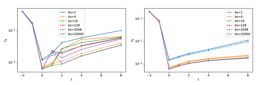
Figure 11: SGD with mini-batches shows the same qualitative behaviour as online learning We show the asymptotic generalisation error $\epsilon_{g}^{*}$ for students with sigmoidal (left) and ReLU activation function (right) for various $K$ learning from a teacher with $M=4$. Between the curves, we change the size of the mini-batch used at each step of SGD from $1$ (online learning) to 20 000. Parameters: $N=500,\eta=0.2,\sigma=0.1,\kappa=0$.

One key characteristic of online learning is that we evaluate the gradient of the loss function using a single sample from the training step per step. In practice, it is more common to actually use a number of samples $b>1$ to estimate the gradient at every step. To be more precise, the weight update equation for SGD with mini-batches would read:

$$w_{k}^{\mu+1}=w_{k}^{\mu}-\frac{\kappa}{N}w_{k}^{\mu}-\frac{\eta}{b\sqrt{N}}\sum_{\ell=1}^{b}x^{\mu,\ell}g^{\prime}(\lambda_{k}^{\mu,\ell})\left[\phi(w,x^{\mu,\ell})-y_{B}^{\mu,\ell}\right].$$ (59)

where $x^{\mu,\ell}$ is the $\ell$th input from the mini-batch used in the $m$th step of SGD, $\lambda_{k}^{\mu,\ell}$ is the local field of the $k$th student unit for the $\ell$th sample in the mini-batch, etc. Note that when we use every sample only once during training, using mini-batches of size $b$ increases the amount of data required by a factor $b$ when keeping the number of steps constant.

We show the asymptotic generalisation error of student networks of varying size trained using SGD with mini-batches and a teacher with $M=4$ in Fig. 11. Two trends are visible: first, using increasing the size of the mini-batches decreases the asymptotic generalisation error $\epsilon_{g}^{*}$ up to a certain mini-batch size, after which the gains in generalisation error become minimal; and second, the shape of the $\epsilon_{g}^{*}-L$ curve is the same for all mini-batch sizes, with the minimal generalisation error attained by a network with $K=M$.

Appendix F Using MNIST images for training and testing

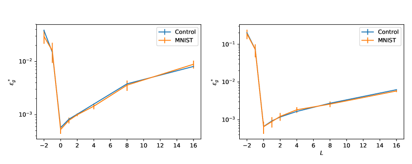
Figure 12: Higher-order correlations in the input data do not play a role for the asymptotic generalisation. WE plot the final generalisation error $\epsilon_{g}^{*}$ after online learning of a student of various sizes from a teacher with $M=4$ using Gaussian inputs (blue) and MNIST images (red) for training and testing. $N=784,\eta=0.1,\sigma=0.1,\kappa=0$.

In the derivation of the ODE description of online learning for the main text, we noted that only the first two moments of the input distribution matter for the learning dynamics and for the final generalisation error. The reason for this is that the inputs only appear in the equations of motion for the order parameters as a product with the weights of either the teacher or the student. Now since they are – by assumption – uncorrelated with those weights, this product is the sum of large number of random variables and hence distributed by the central limit theorem.

We have checked how our results change when this assumption breaks down in one example where we train a network on a finite data set with non-trivial higher order moments, namely the images of the MNIST data set. We studied the very same setup that we discuss throughout this work, namely the supervised learning of a regression task in the teacher-student scenario. We only replace the the inputs, which would have been i.i.d. draws from the standard normal distribution, with the images of the MNIST data set. In particular, this means that we do not care about the labels of the images. Figure 12 shows a plot of the resulting final generalisation against $L$ for both the MNIST data set and a data set of the same size, comprised of i.i.d. draws from the standard normal distribution, which are in good agreement.

Appendix G Early-stopping generalisation error for finite training sets

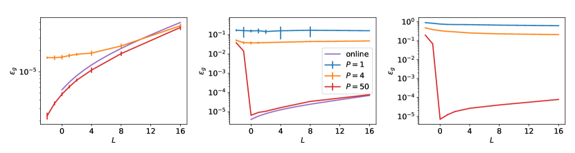
Figure 13: The scaling of $\epsilon_{g}^{*}$ with $L$ shows a similar dependence on the size of the training set for early-stopping (top) and final (bottom) generalisation error. We plot the asymptotic and the early-stopping generalisation error after SGD with a finite training set containing $PN$ samples (linear, sigmoidal and ReLU networks from left to right). The result for online learning for linear and sigmoidal networks, Eqns. 13 and 15 of the main text, are plotted in violet. Error bars indicate one standard deviation over 10 simulations, each with a different training set; many of them are too small to be clearly visible. Parameters: $N=784,M=4,\eta=0.1,\sigma=0.01$.

A common way to prevent over-fitting of a neural network when training with a finite training set in practice is early stopping, where the training is stopped before the training error has converged to its final value yet. The idea behind early-stopping is thus to stop training before over-fitting sets in. For the purpose of our analysis of the generalisation of two-layer networks trained on a fixed finite data set in Sec. 4 of the main text, we define the early-stopping generalisation error $\hat{\epsilon}_{g}$ as the minimum of $\epsilon_{g}$ during the whole training process. In Fig. 13, we reproduce Fig. 6 from the main text at the bottom and plot $\hat{\epsilon}_{g}$ obtained from the very same experiments at the top. While the ReLU networks showed very little to no over-training, the sigmoidal networks showed more significant over-training. However, the qualitative dependence of the generalisation errors on $L$ was observed to be the same in this experiment. In particular, the early-stopping generalisation error also shows two different regimes, one where increasing the network hurts generalisation ($P\gg K$), and one where it improves generalisation or at least doesn’t seem to affect it much (small $P\sim K$).

Appendix H Explicit form of the integrals appearing in the equations of motion of sigmoidal networks

To be as self-contained as possible, here we collect the explicit forms of the integrals $I_{2}$, $I_{3}$, $I_{4}$ and $J_{2}$ that appear in the equations of motion for the order parameters and the generalisation error for networks with $g(x)=\operatorname{erf}\left(x/\sqrt{2}\right)$, see Eq. (37). They were first given by [15, 16]. Each average $\langle\cdot\rangle$ is taken w.r.t. a multivariate normal distribution with mean 0 and covariance matrix $C\in\mathbb{R}^{n}$, whose components we denote with small letters. The integration variables $u,v$ are always components of $\lambda$, while $w$ and $z$ can be components of either $\lambda$ or $\nu$.

$$J_{2} \equiv\langle g^{\prime}(u)g^{\prime}(v)\rangle=\frac{2}{\pi}{\left(1+c_{11}+c_{22}+c_{11}c_{22}-c_{12}^{2}\right)}^{-1/2}$$ (60)

$$I_{2} \equiv\frac{1}{2}\langle g(w)g(z)\rangle=\frac{1}{\pi}\arcsin\frac{c_{12}}{\sqrt{1+c_{11}}\sqrt{1+c_{12}}}.$$ (61)

$$I_{3} \equiv\langle g^{\prime}(u)wg(z)\rangle=\frac{2}{\pi}\frac{1}{\sqrt{\Lambda_{3}}}\frac{c_{23}(1+c_{11})-c_{12}c_{13}}{1+c_{11}}$$ (62)

$$I_{4} \equiv\langle g^{\prime}(u)g^{\prime}(v)g(w)g(z)\rangle=\frac{4}{\pi^{2}}\frac{1}{\sqrt{\Lambda_{4}}}\arcsin\left(\frac{\Lambda_{0}}{\sqrt{\Lambda_{1}\Lambda 2}}\right)$$ (63)

where

$$\Lambda_{4}=(1+c_{11})(1+c_{22})-c_{12}^{2}$$ (64)

and

$$\Lambda_{0} =\Lambda_{4}c_{34}-c_{23}c_{24}(1+c_{11})-c_{13}c_{14}(1+c_{22})+c_{12}c_{13}c_{24}+c_{12}c_{14}c_{23}$$ (65)

$$\Lambda_{1} =\Lambda_{4}(1+c_{33})-c_{23}^{2}(1+c_{11})-c_{13}^{2}(1+c_{22})+2c_{12}c_{13}c_{23}$$ (66)

$$\Lambda_{2} =\Lambda_{4}(1+c_{44})-c_{24}^{2}(1+c_{11})-c_{14}^{2}(1+c_{22})+2c_{12}c_{14}c_{24}$$ (67)

References

- [1] Y. LeCun, Y. Bengio, and G. E. Hinton. Deep learning. Nature, 521(7553):436–444, 2015.
- [2] V. Mnih, K. Kavukcuoglu, D. Silver, A.A. Rusu, J. Veness, M.G. Bellemare, A. Graves, M. Riedmiller, A.K. Fidjeland, G. Ostrovski, S. Petersen, C. Beattie, A. Sadik, I. Antonoglou, H. King, D. Kumaran, D. Wierstra, S. Legg, and D. Hassabis. Human-level control through deep reinforcement learning. Nature, 518(7540):529–533, 2015.
- [3] D. Silver, A. Huang, C.J. Maddison, A. Guez, L. Sifre, G. van den Driessche, J. Schrittwieser, I. Antonoglou, V. Panneershelvam, M. Lanctot, S. Dieleman, D. Grewe, J. Nham, N. Kalchbrenner, I. Sutskever, T. Lillicrap, M. Leach, K. Kavukcuoglu, T. Graepel, and D. Hassabis. Mastering the game of Go with deep neural networks and tree search. Nature, 529(7587):484–489, 2016.
- [4] K. Simonyan and A. Zisserman. Very Deep Convolutional Networks for Large-Scale Image Recognition. In International Conference on Learning Representations, 2015.
- [5] P.L. Bartlett and S. Mendelson. Rademacher and Gaussian complexities: Risk bounds and structural results. Journal of Machine Learning Research, 3(3):463–482, 2003.
- [6] Mehryar Mohri, Afshin Rostamizadeh, and Ameet Talwalkar. Foundations of Machine Learning. MIT Press, 2012.
- [7] B. Neyshabur, R. Tomioka, and N. Srebro. Norm-Based Capacity Control in Neural Networks. In Conference on Learning Theory, 2015.
- [8] N. Golowich, A. Rakhlin, and O. Shamir. Size-Independent Sample Complexity of Neural Networks. arxiv:1712.06541, 2017.
- [9] G.K. Dziugaite and D.M. Roy. Computing Nonvacuous Generalization Bounds for Deep (Stochastic) Neural Networks with Many More Parameters than Training Data. In Proceedings of the Thirty-Third Conference on Uncertainty in Artificial Intelligence, 2017.
- [10] S. Arora, R. Ge, B. Neyshabur, and Yi Zhang. Stronger generalization bounds for deep nets via a compression approach. arxiv:1802.05296, 2018.
- [11] Z. Allen-Zhu, Y. Li, and Y. Liang. Learning and Generalization in Overparameterized Neural Networks, Going Beyond Two Layers. arXiv:1811.04918, 2018.
- [12] B. Neyshabur, R. Tomioka, and N. Srebro. In search of the real inductive bias: On the role of implicit regularization in deep learning. In ICLR, 2015.
- [13] C. Zhang, S. Bengio, M. Hardt, B. Recht, and O. Vinyals. Understanding deep learning requires rethinking generalization. In ICLR, 2017.
- [14] D. Arpit, S. Jastrz, M. S. Kanwal, T. Maharaj, A. Fischer, A. Courville, and Y. Bengio. A Closer Look at Memorization in Deep Networks. In Proceedings of the 34th International Conference on Machine Learning, 2017.
- [15] M. Biehl and H. Schwarze. Learning by on-line gradient descent. J. Phys. A. Math. Gen., 28(3):643–656, 1995.
- [16] D. Saad and S.A. Solla. Exact Solution for On-Line Learning in Multilayer Neural Networks. Phys. Rev. Lett., 74(21):4337–4340, 1995.
- [17] D. Saad and S.A. Solla. On-line learning in soft committee machines. Phys. Rev. E, 52(4):4225–4243, 1995.
- [18] E. Gardner and B. Derrida. Three unfinished works on the optimal storage capacity of networks. Journal of Physics A: Mathematical and General, 22(12):1983–1994, 1989.
- [19] H. S. Seung, H. Sompolinsky, and N. Tishby. Statistical mechanics of learning from examples. Physical Review A, 45(8):6056–6091, 1992.
- [20] T. L. H. Watkin, A. Rau, and M. Biehl. The statistical mechanics of learning a rule. Reviews of Modern Physics, 65(2):499–556, 1993.
- [21] A. Engel and C. Van den Broeck. Statistical Mechanics of Learning. Cambridge University Press, 2001.
- [22] L. Zdeborová and F. Krzakala. Statistical physics of inference: thresholds and algorithms. Adv. Phys., 65(5):453–552, 2016.
- [23] M. S. Advani and S. Ganguli. Statistical mechanics of optimal convex inference in high dimensions. Physical Review X, 6(3):1–16, 2016.
- [24] P. Chaudhari, A. Choromanska, S. Soatto, Y. LeCun, C. Baldassi, C. Borgs, J. Chayes, L. Sagun, and R. Zecchina. Entropy-SGD: Biasing Gradient Descent Into Wide Valleys. In ICLR, 2017.
- [25] M. Advani and A. M. Saxe. High-dimensional dynamics of generalization error in neural networks. arXiv:1710.03667, 2017.
- [26] B. Aubin, A. Maillard, J. Barbier, F. Krzakala, N. Macris, and L. Zdeborová. The committee machine: Computational to statistical gaps in learning a two-layers neural network. In Advances in Neural Information Processing Systems 31, pages 3227–3238, 2018.
- [27] M. Baity-Jesi, L. Sagun, M. Geiger, S. Spigler, G.B. Arous, C. Cammarota, Y. LeCun, M. Wyart, and G. Biroli. Comparing Dynamics: Deep Neural Networks versus Glassy Systems. In Proceedings of the 35th International Conference on Machine Learning, 2018.
- [28] H. Schwarze. Learning a rule in a multilayer neural network. Journal of Physics A: Mathematical and General, 26(21):5781–5794, 1993.
- [29] G. Cybenko. Approximation by superpositions of a sigmoidal function. Math. Control. Signals Syst., 2(4):303–314, 1989.
- [30] K. Hornik, M. Stinchcombe, and H. White. Multilayer feedforward networks are universal approximators. Neural Networks, 2(5):359–366, 1989.
- [31] S. Mei, A. Montanari, and P.-M. Nguyen. A mean field view of the landscape of two-layer neural networks. Proceedings of the National Academy of Sciences, 115(33):E7665–E7671, 2018.
- [32] G. M. Rotskoff and E. Vanden-Eijnden. Parameters as interacting particles: long time convergence and asymptotic error scaling of neural networks. In Advances in neural information processing systems 31, pages 7146–7155, 2018.
- [33] L. Chizat and F. Bach. On the global convergence of gradient descent for over-parameterized models using optimal transport. In Advances in Neural Information Processing Systems 31, pages 3040–3050, 2018.
- [34] Y. Li and Y. Liang. Learning Overparameterized Neural Networks via Stochastic Gradient Descent on Structured Data. In Advances in Neural Information Processing Systems 31, 2018.
- [35] W. Kinzel and P. Ruján. Improving a Network Generalization Ability by Selecting Examples. EPL (Europhysics Letters), 13(5):473–477, 1990.
- [36] C.W.H. Mace and A.C.C. Coolen. Statistical mechanical analysis of the dynamics of learning in perceptrons. Statistics and Computing, 8(1):55–88, 1998.
- [37] D. Saad and S.A. Solla. Learning with Noise and Regularizers Multilayer Neural Networks. In Advances in Neural Information Processing Systems 9, pages 260–266, 1997.
- [38] E. Oja and J. Karhunen. On stochastic approximation of the eigenvectors and eigenvalues of the expectation of a random matrix. Journal of Mathematical Analysis and Applications, 106(1):69–84, 1985.
- [39] C. Wang, J. Mattingly, and Yue M. Lu. Scaling Limit: Exact and Tractable Analysis of Online Learning Algorithms with Applications to Regularized Regression and PCA. arXiv:1712.04332, 2017.
- [40] C. Wang, H. Hu, and Y. M. Lu. A Solvable High-Dimensional Model of GAN. arXiv:1805.08349, 2018.
- [41] A. Brutzkus, A. Globerson, E. Malach, and S. Shalev-Shwartz. SGD learns over-parameterized networks that provably generalize on linearly separable data. In International Conference on Learning Representations, 2018.
- [42] M. Soltanolkotabi, A. Javanmard, and J.D. Lee. Theoretical insights into the optimization landscape of over-parameterized shallow neural networks. IEEE Transactions on Information Theory, 65(2):742–769, 2018.
- [43] A. Krogh and J. A. Hertz. Generalization in a linear perceptron in the presence of noise. Journal of Physics A: Mathematical and General, 25(5):1135–1147, 1992.
- [44] A.M. Saxe, J.L. McClelland, and S. Ganguli. Exact solutions to the nonlinear dynamics of learning in deep linear neural networks. In ICLR, 2014.
- [45] A.K. Lampinen and S. Ganguli. An analytic theory of generalization dynamics and transfer learning in deep linear networks. In International Conference on Learning Representations, 2019.