A Kalman filtering induced heuristic optimization based partitional data clustering
Abstract
Clustering algorithms have regained momentum with recent popularity of data mining and knowledge discovery approaches. To obtain good clustering in reasonable amount of time, various meta-heuristic approaches and their hybridization, sometimes with K-Means technique, have been employed. A Kalman Filtering based heuristic approach called Heuristic Kalman Algorithm (HKA) has been proposed a few years ago, which may be used for optimizing an objective function in data/feature space. In this paper at first HKA is employed in partitional data clustering. Then an improved approach named HKA-K is proposed, which combines the benefits of global exploration of HKA and the fast convergence of K-Means method. Implemented and tested on several datasets from UCI machine learning repository, the results obtained by HKA-K were compared with other hybrid meta-heuristic clustering approaches. It is shown that HKA-K is atleast as good as and often better than the other compared algorithms.
keywords:
Clustering, K-Means, Optimization, Metaheuristic Optimization, Heuristics1 Introduction
Clustering is the process of assigning a set of data points into classes based on the similarity between the data points in the feature space. It is useful when some prototype data from known classes are not available for training a supervised classifier or for an exploratory data analysis task. It is one of the earliest pattern classification approaches and has found renewed interest since the beginning of data mining and big data analytics.
Clustering can be broadly classified into two categories: Hierarchical and Partitional. Hierarchical clustering methods are again grouped into two types, namely divisive or top-down and agglomerative or bottom-up methods. If the number of desired clusters is known (say, ) a priori, the approach can be made non-hierarchical and the data can be assigned into clusters using a partitional clustering algorithm. Else, several clusterings are generated and the best among them is chosen on the basis of some objective criterion.
One of the classical partitional clustering approaches is the K-Means algorithm, which is a simple way to discover convex, especially hyper-spherical clusters. It starts with seed points in the feature space representing the initial cluster centers. Then it assigns a data point to the cluster whose center is nearest to . When all data are assigned in such a way, the centers are updated by the mean position of current data assigned to each cluster. Then a new iteration starts and the data are redistributed using the nearness criterion stated above. The process is repeated till the centroids do not change anymore or a specified number of iterations is reached.
However, K-Means approach may fail to find desired results for some choice of initial seed points. In such a case it converges to a local sub-optimal solution, or may even fail to converge [38]. One of the various techniques proposed to tackle the problem model the clustering task as a non-convex optimization problem employing a cluster quality based objective function and then try to find its global optimum. Since finding such an optimum is an NP-Complete problem [40], metaheuristic algorithms are employed, among others, to find a near optimal solution. A metaheuristic algorithm only uses values of the objective function to be optimised and does not require the function to have derivatives. Hence, metaheuristic algorithms are one of the choices to optimize the non-convex optimization problems. Examples of metaheuristic based methods are PSO (Particle Swarm Optimization), GA (Genetic Algorithm), ACO (Ant Colony Optimization) etc. Another class of algorithms are based on hybrid approach, where two or more metaheuristic algorithms are combined, or metaheuristic algorithms are combined with K-Means or other local search methods. Some examples of this category are hybrid of K-Means and PSO, hybrid of K-Means and GA as well as PSO-ACO-K-Means hybrid algorithms. A review on different clustering techniques can be found in [18], while a survey of metaheuristic algorithms is given in [30]. A brief survey of metaheuristic based clustering algorithms will be presented in Section 2 of this paper.
A new metaheuristic based optimization approach named Heuristic Kalman Algorithm (HKA) has been proposed by Toscano and Lyonnet in [41]. This method uses a random number generator with Gaussian probability distribution to choose a set of points in the search space. At each subsequent iteration, the mean vector and covariance matrix for the Gaussian random number generator are modified using a Kalman filtering framework, so that the mean gets nearer to the global optimum.
In the past, HKA has been employed in applied problems like tuning of PID controllers [41] and in robust observer for rotor flux estimation of induction machine [42]. The present paper uses HKA for data clustering context. More specifically, the contributions of this paper are as follows.
-
1.
To employ HKA for data clustering and show that it performs well on synthetic and real datasets.
-
2.
To propose an improvement over the above HKA based approach through hybridization with a K-Means like approach. The proposed approach is named HKA-K where the K indicates application of K-Means like approach. It is demonstrated that HKA-K converges faster than HKA.
-
3.
To demonstrate that the performance of HKA-K in terms of accuracy, convergence and computational efficiency is as good as or better than several other state of the art metaheuristic based clustering algorithms.
The rest of the paper is organized as follows. We briefly survey the metaheuristic algorithms and hybrid metaheuristic algorithms for data clustering in Section 2. In Section 3 the HKA based optimization approach is explained by following the paper [41]. A brief exposition of partitional clustering, along with centroid based K-Means approach is provided in Section 4. The approach of using HKA to data clustering is introduced in the same section. Then the proposed improvement on HKA clustering, namely HKA-K approach is developed in Section 5. Experimental results are presented and discussed in Section 6 where comparisons are also made with other metaheuristic based methods. Section 7 contains some concluding remarks on the paper.
2 Brief survey on metaheuristic based clustering
Metaheuristic population based optimization algorithms in general are used in clustering either as is, or as a hybrid variant combining multiple algorithms. In general two or more population based algorithm and/or a local search algorithm are combined together.
Among pure and hybrid metaheuristic based clustering approaches, a Genetic Algorithm (GA) based approach named COWCLUS [9] was presented, which uses Calinski and Harabasz Variance Ratio Criteria [5] as the cost function and performs standard GA to optimize it. Another approach in [29] has used GA to optimize the clustering objective function. Yet another GA based approach named GKA [23] has introduced a new mutation operator and combined it with K-Means for better convergence. These early methods consider each chromosome representing a clustering of the data points. The chromosome has alleles, each taking an integer value corresponding to one particular cluster. On the other hand, the GA based method KGA [27] encodes only the cluster centers in the chromosomes as real numbers. In this case if clusters are to be obtained on -dimensional data, each chromosome will have a length of . This method combines K-Means and GA and is more effective than the previous ones. A Differential Evolution (DE) and K-Means based algorithm was proposed in [26], where the K-Means method is used to refine the results given by the recombination operators of DE.
Particle Swarm Optimization (PSO) has also been employed for data clustering [34, 19, 32]. PSO was hybridized with K-Means in [2, 10, 43, 34] to improve convergence. In [46] a Gaussian based distance metric [45] was used while clustering the data using PSO algorithm. Also, an approach combining GA and PSO is given in [25]. Another hybrid algorithm [24] employs GA, PSO and K-Means approach to determine the number of clusters as well as to perform clustering.
Among other metaheuristic approaches, Artificial Bee Colony (ABC) optimization [20, 21] was applied for clustering data [22, 47]. Also, an Ant Colony Optimization (ACO) based technique was proposed in [39]. In [31] an approach involving PSO, ACO and K-Means while in [33] an ACO and Simulated Annealing (SA) based algorithm was proposed. The swarm based approach with honey-bee mating process named Honey Bee Mating Optimization (HBMO) [1] was used in clustering domain [14].
Clustering was done with Artificial Fish Swarm (AFS) algorithm [48, 7] and Bacteria Foraging Algorithm (BFO) [44] as well. Clustering using Cuckoo Search approach was also proposed in [36]. Moreover, an automatic clustering using Invasive Weed Optimization (IWO) can be found in [8]. A new method, Gravitational Search Algorithm (GSA), proposed in [35], was used to cluster data [16]. Another approach called Black-Hole search, was also applied in data clustering [15].
In the following section we briefly introduce HKA and then explain how it can be used for clustering.
3 Heuristic Kalman Algorithm (HKA)
The HKA [41] is a non-convex, population-based, metaheuristic optimization algorithm, which works in a manner different from other population based metaheuristic approaches. Let an objective function be defined over a multidimensional and bounded real space . We have to find the position of a point in where the value of is optimum. The HKA based approach in [41] for finding this point is described below.
A solution is generated through a Gaussian probability density function (pdf), where the mean vector represents the position in and the variance matrix represents the uncertainty of the solution. Given a search space , the objective of the algorithm is to modify the mean and variance matrix of a Gaussian pdf at iteration such that the mean ideally approaches the global optima within with respect to the objective function , along with decreasing variance. The modification of the mean and variance matrix is done by an approach based on Kalman filtering. The algorithm starts with an initial mean vector and variance matrix . The computation of the initial values are explained later. At each iteration the measurement step generates number of points given by vectors from a Gaussian pdf , which are ordered such that is satisfied. Another Gaussian pdf is generated by taking the mean (Eq. (1)) of the vector positions of top number of points, and the variance (Eq. (2)) is computed on these top points. This is considered to be the measurement. Next, in the estimation step, the Kalman filter is used to combine these two Gaussian pdfs to generate a new Gaussian pdf , where is expected to be closer to the desired solution than . Here is computed using Eq. (3), (4) and (5) while is computed using Eq. (5), (6), (7) and (8). If a stopping condition is encountered, then it takes the so far found best value of , else it carries the Gaussian pdf computed for the estimation step in the next iteration and repeats the process.
It should be mentioned that, in the current formulation, the matrices and contain only the diagonal elements and hence can also be treated as vector of dimension , which is the dimension of the feature space .
The value of is calculated as
| (1) |
Also, the uncertainty matrix is given by
| (2) |
The estimation step computes the parameters , for Gaussian pdf for next iteration by
| (3) |
| (4) |
| (5) |
| (6) |
| (7) |
Here is the predicted covariance matrix and is the Kalman gain. The details of Kalman filter and Kalman gain can be found in [28, 13]. A slowdown factor is introduced here to control the fast decrease of the covariance matrix, which otherwise could converge prematurely to a bad solution. The factor is defined as
| (8) |
In Eq (8), is the slowdown co-efficient, which is a parameter of the algorithm, and and are the diagonal of the matrices and respectively.
The process is repeated till the value of reaches a predefined number, or the best solutions generated at some iteration is within a hypersphere with a predefined radius , centered about the best of the generated vectors . In both cases, the found best is declared as the solution.
The initial value of and in HKA are computed as follows.
| (9) |
| (10) |
Here is the component of the mean vector, is the diagonal of the variance matrix, while and indicate the maximum and minimum bound value along the dimension of the search space .
The convergence properties and other analysis of HKA can be found in [41] where the authors have shown that HKA performs well with respect to several test functions and attains better results than other algorithms most of the time. The authors of HKA in [41] have also shown that the number of function evaluations to reach the solution for HKA is lower than a few other metaheuristic optimization algorithms and this method was able to reach better results most of the time. Also, constrained optimization was demonstrated by the authors in solving the welded beam design problem and in tuning Proportional Integral Derivative (PID) controllers.
4 Partitional clustering using HKA
4.1 Partitional Clustering
Assume a dataset , where , is a datum represented as a vector in -dimensional feature space. The task of clustering is to partition into a set of clusters such that cluster contains data points similar to each other and dissimilar to the data of other clusters with respect to some measure of similarity. In crisp partitional clustering all clusters should be non-empty , and having no common elements where , and while .
The centroids for the set are where is given by Eq. (11)
| (11) |
where , and is the cardinality of the set .
Several algorithms consider clustering as a global optimization problem, where one or more objective functions representing the cluster quality is optimized. Here we have used the sum of squared intra-cluster Euclidean distances as the objective function to minimize, which is given by
| (12) |
Where is the magnitude of the vector in Euclidean space, and is the cluster assignment value defined as
where and .
Therefore the objective is to optimize Eq. (12) with respect to , on a fixed dataset , and find the cluster assignment for all and .
Since we have used the “idea” of K-Means algorithm in our HKA-K approach, a brief description of K-Means algorithm is given below.
-
1.
The number of clusters is prespecified. Initially, the set of cluster centers is randomly generated.
-
2.
A data point is assigned to if is closest to , ie. , where and . All datapoints are assigned in this way.
-
3.
Using Eq. (11), the cluster center is updated with the datapoints assigned to the cluster in Step 2. All the cluster centers are updated in this way.
-
4.
If a termination criterion is satisfied, then the process is stopped. Else, the control goes to Step 2 with current cluster centers.
A detailed analysis of K-Means approach can be found in [4].
4.2 HKA based partitional clustering
For our purpose we represent the cluster centers as a concatenated vector. If the cluster centers are in , then the concatenated vector will be , where denotes the concatenation of the comma separated vectors. Clearly, the dimension of vector will be . To compute the objective value for such a concatenated vector, the individual s are extracted from and Eq. (12) is used.
The clustering process progresses as in the HKA algorithm. It starts with an initial mean and covariance matrix for the Gaussian random number generator. is set to . In every iteration , the process generates random vectors from a Gaussian pdf with mean vector and covariance matrix and , respectively. Next, it computes using Eq. (1) and using Eq. (2) and then estimates using Eq. (3) and using Eq. (6) and (5). If the objective value of is better than then it is updated with . For the next iteration, and are computed as in Eq. (4) and Eq. (7) respectively, and is incremented. This process is repeated until the value of reaches some prefixed number of iterations, or the best samples generated in some iteration is within a hypersphere of a predefined radius , centered at the best sample point. When terminated, is taken as the solution. Here, , , and the generated vectors from the Gaussian pdfs are encoded as described in the previous paragraph.
For initialization, is chosen in a similar way as in HKA but here the search space is considered as the minimum bounding hyperbox of the dataset.
| (13) |
Here is the concatenation of the vector , times. (and denotes the maximum (and minimum) value of dimension over all datapoints in the dataset.
The initial covariance matrix is taken as
| (14) |
| (15) |
Given a dataset, the minimum bounding hyperbox will contain all the data points inside the hyperbox. As we are performing a centroid based clustering task and the cluster centers cannot be outside this bounding box, the algorithm does not need to search outside this hyperbox. Therefore we select the starting point of the search at the center of the minimum bounding hyperbox and select a variance which is sufficiently large so that the random samples covers almost the entire search space. Also, we limit the search so that the search does not cross this hyperbox.
5 HKA-K Clustering
Though HKA performs fairly well for clustering data, as shown in Section 6, it would be interesting to see if the results could be improved. Improvement can be envisioned on two aspects, namely accuracy of the results and efficiency of the algorithm. One possible way of achieving both is to exploit global search nature of the algorithm combined with a local search. We have tried to attain this by exploiting the simplicity and speed of K-Means approach under a hybrid framework. A centroid based K-Means like step is used because of its simplicity. A full K-Means algorithm is not run, instead we only use one single step of centroid updates with the K-Means approach at each iteration.
In this work we make the following two modifications: (a) we introduce a new step after the estimation step of HKA with a view to attain faster convergence and better accuracy, (b) we incorporate a restart mechanism which in effect attempts to avoid the search getting trapped in a local optimum or stagnation. We show that these modifications are effective in improving convergence and speed compared to HKA based clustering as well as several other state-of-the-art metaheuristic based clustering algorithms.
For the above process, we introduce a time update step which updates the estimated through one single step of weighted K-Means operator. The estimated is also updated accordingly. See [28, 13] for time update in Kalman filtering approach. On the other hand, in HKA the estimated is directly used in the next iteration (Eq. (4)). By the term K-Means operator we mean one single iteration of K-Means which will update the centroids to move towards the solution, we control this movement through weight. We also introduce a conditional restart mechanism. The search is restarted if the sample points fall in a small region limited by a constant .
- 1.
-
2.
Step 2, Randomly generate number of -dimensional vectors from Gaussian pdf .
- 3.
- 4.
- 5.
-
6.
Step 6, If then set , else set
- 7.
-
8.
Step 8, If then terminate the algorithm. Output as the solution. Else set , goto Step 2
Algorithm 1 describes HKA-K in steps. After initialization in Step 1, vectors are generated in Step 2 randomly from the Gaussian pdf at the iteration using the mean and covariance matrix . In this context, the mean and covariance matrix are the parameters to the Gaussian pdf which is modified by the Kalman filter framework as in HKA. These parameters should not to be confused with the mean or covariance matrix of the data set.
Next, in Step 3, the measurement is taken by finding the mean value of the points as in Eq. (1) and the measurement error by Eq. (2). Next Eq. (3), (5), (6) are used to get the state update and the related variance in Step 4. The time update is performed at Step 5, where at first each of the cluster centroids in are extracted from the vector representation and the K-Means operator is used to get the centers are obtained. Now, the centers for the next iteration is given by
| (16) |
The weight used to control the influence of K-Means can be a constant or a function. For our experiments we took as a constant number in the interval . A moderate value of should be selected such that the effect of HKA and K-Means are balanced.
From the Kalman filtering algorithm, ignoring the control inputs and process noise, the state and its related covariance matrix for the next iteration can be obtained as
| (17) |
| (18) |
Here is the state transition matrix. The related covariance matrix is updated as shown in Eq. (18). We find by Eq. (16) and hence to update the covariance matrix we need to find . We consider to be a diagonal matrix with the components given by
| (19) |
Where is the diagonal component of . Conversely in HKA, is considered identity matrix and is equal to . Now is used to update the variance by Eq. (18). The mean is used in the next iteration and is computed from after a slowdown step in Eq. (20) is used in the next iteration with the Gaussian pdf.
In each iteration the best vector found so far is retained in Step 6, which indicates the optimum value of found till the current iteration. The initial value is set to . If then is set to . Otherwise, is retained as . Note that we use the un-weighted K-Means step to store the best vector, while employ weighted updating for further search.
The slowdown factor is computed as done in HKA. Therefore the variance matrix update after the modification along with slowdown becomes
| (20) |
The restart stage, Step 7 works as follows. At first, the top vectors from the measurement step are scaled within the range to get . Then the maximum Euclidean distances of the vectors centered around the best point , is computed. Finally, the distance is scaled by dividing the number of dimensions to get
| (21) |
If drops below a predefined parameter , an input to the algorithm, then the search is restarted. Instead of using the previously mentioned initialization, to start exploring from a different location, the restart is done by selecting number of random datapoints selected uniformly from the dataset and concatenating them to get a new vector and the restarted variance for the restarted process, as in Eq. (14) and (15).
Step 8 terminates the algorithm and takes as a solution, if the iterations exceeds the . Else, the control goes to Step 2.
6 Experiment
6.1 Used Dataset
To test the usefulness of the proposed HKA-K and HKA clustering algorithms, we have performed experiments with two synthetic datasets and a few well known datasets from the UCI Machine Learning repository [3]. We have also compared the performance of HKA-K with some population based hybrid algorithms. All the algorithms were implemented with C++ using Armadillo [37] linear algebra library. Table 1 lists the datasets used in our experiment and provides the number of points , dimensionality and the number of clusters present in the data .
| Artset1 | Artset2 | Iris | Wine | Glass | CMC | Cancer | |
|---|---|---|---|---|---|---|---|
| No. of Data: | 600 | 250 | 150 | 178 | 214 | 1473 | 683 |
| Dimensions: | 2 | 3 | 4 | 13 | 9 | 9 | 9 |
| Clusters: | 6 | 5 | 3 | 3 | 6 | 3 | 2 |
The datasets acquired from the UCI machine learning repository listed in Table 1 were chosen because these datasets are quite frequently used in clustering related literature.The synthetic datasets Artset1 and Artset2 are generated as follows.
-
1.
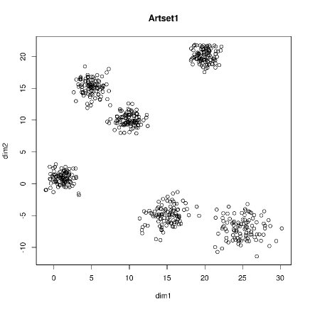
Artset1 : This two-dimensional dataset consists of 6 clusters. The plot of this dataset is shown in Figure 1a. Here 600 patterns were drawn from six independent bi-variate normal distributions, with the mean and covariances given by
, , , , , . A scatterplot for these datapoints are shown in Figure 1a. -
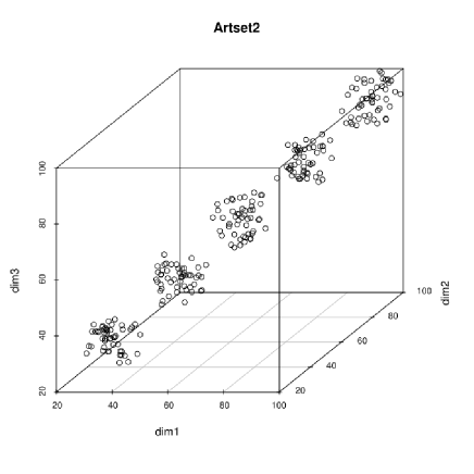
2.
Artset2 : This three-dimensional synthetic dataset consists of 5 clusters. The plot of this dataset is shown in Figure 1b. Each dimension of the dataset is class-wise distributed as Class 1 - Uniform(85, 100), Class 2 - Uniform(70, 85), Class 3 - Uniform(55, 70) Class 4 - Uniform(40, 55), Class 5 - Uniform(25, 40), where each class has 50 datapoints. A scatterplot for these datapoints are shown in Figure 1b.
6.2 Used Parameters
We have tested HKA-K and HKA clustering algorithms, as well as, KGA [27], GAC [23], ABCC [22] and PSO [6] algorithms on the above datasets and compared the results. For all the algorithms, the optimization criterion used is Eq. (12).
For conducting the experiments, the parameters for HKA clustering and HKA-K are selected as follows. At first, HKA was run on Glass dataset with different combinations of , and , while HKA-K was run with different combinations of , , and . Then the parameter combination with the minimum sum of intra-cluster distances over 10 executions, (with each execution having a maximum of 250 iterations) was selected. These parameter values, given in the first two columns of Table 2 have been used for the clustering of all other datasets.
Table 2 also shows the parameters used for other four methods with which we compared our algorithm. The Tables 3-9 show the results for all the methods with the prescribed parameters listed in Table 2, which are taken from the corresponding referenced articles. The parameters for KGA and GAC are taken from [27] (though more iterations were added to GAC). We have used the parameters for ABCC from [22], while the parameters for the PSO algorithm [6] were taken from [31] instead, as we found PSO clustering in [6] performed better with these parameters. All of the KGA, GAC, PSO, ABCC algorithms were executed 20 times with the corresponding parameters and the results are shown in Tables 3-9. These were used to show how HKA-K and HKA clustering performs when compared to other algorithms under parameters prescribed by the authors of the corresponding algorithms. It is very important to note that the number of function evaluations highly differ to each other for each algorithms for the given selection of parameters. We have performed this test to understand the achievable cluster quality of the algorithms.
On the other hand we have performed another experiment with the parameters mentioned in Table 10 which were selected in such a way that all the algorithms approximately runs equal number of objective function evaluations. The number of function evaluations for all the algorithms are kept almost equal to HKA-K in this experiment. This is done to see how the algorithms converge when all of them evaluate approximately equal number of functions. Details are explained in Section 6.4.
In Table 2 and Table 10, is the population size for KGA, GAC and PSO, while and are the crossover and mutation probability, respectively, for both KGA and GAC. The parameter indicates the number of generations the algorithms KGA and GAC are allowed to run. The parameters and are the cognitive and social factors, and the and are minimum and maximum momentum factors for PSO. The parameter is the number of food sources to exploit and is the limit of the food source for ABCC algorithm. Also, is the number of maximum iterations taken for HKA-K, HKA clustering, ABCC and PSO algorithms.
6.3 Evaluation Metrics
We have used several metrics to estimate and compare the cluster quality, which are of two types, namely internal and external. The internal metrics assume that the datapoints within the clusters are close, compact and hyper-spherical while different clusters are well separated, but they do not use the true class labels into consideration. On the other hand, external metrics employ actual class labels of the dataset. After the algorithm assigns the data points to the clusters, the quality is measured using the true class labels of the data.
We have used Adjusted Rand Index (ARI) [17] as an external validation index. For ARI, higher value indicates better clustering and the value indicates best result. The ARI is computed as follows.
Let be the set of clusters found by the algorithm while defines the true class label. Let be the total number of datapoints. Also, let
-
1.
: Number of pairs of datapoints which are placed in a single cluster in and also belongs to a single class in .
-
2.
: Number of pairs of datapoints which are placed in a single cluster in but belongs to different classes in .
-
3.
: Number of pairs of datapoints which are placed in different clusters in but belongs to a single class in .
-
4.
: Number of pairs of datapoints which are placed in different clusters in and also belongs to different classes in .
Then the is defined as
| (22) |
We have also shown the sum of intra-cluster distances (denoted as “Intra” in the tables) of the datapoints and Davies-Bouldin index [11] as internal validation metrics. Of them, the sum of intra-cluster distances (Intra) indicate the compactness of the clusters, denoted as
| (23) |
In Tables 3-9 the rows labeled Intra, the mean, min, max and std respectively denote the mean, minimum, maximum and the standard deviation of over the total number of runs for the experiment. Also, the Table 11 states the mean and standard deviations of the values.
On the other hand, Davies-Bouldin index finds the ratio of the sum of within cluster scatter to the between cluster separation. This metric assumes compact and well separated clusters as ideal. Here, a lower index value indicates better clustering. Davies-Bouldin index is defined as:
where
is a similarity measure between clusters and . This is computed based on the measure of dispersion and of each of and respectively, and the dissimilarity between two clusters , which are defined as follows:
; ;
6.4 Experimental Results
The experimental results are presented and evaluated in two ways as follows. (a) At first, we have presented clustering performance of the algorithms using the parameters prescribed in the referenced articles of the other algorithms. We have shown that HKA-K and HKA clustering can reach similar results in lesser time than the other methods. (b) Next, we have shown that the performance of our HKA-K algorithm is similar to KGA and better than other algorithms when all algorithms are allowed to run for approximately similar number of function evaluations, with nearly the same execution time.
(a) Results with parameters from referenced articles
The parameters selected for this experiment is mentioned in Table 2 and explained in Section 6.2. The results obtained by other methods as well as HKA-K and HKA clustering for different datasets are systematically shown in Table 3-9. In these tables the best results are shown in bold numerals.
At first, let us compare between HKA and HKA-K methods. From the tables it is noted that on all datasets the maximum number of iterations and the population size for HKA-K are smaller than HKA clustering method. Hence HKA-K was able to work faster and attain similar results with respect to the ARI values for Iris, Wine, Cancer and CMC dataset, and slightly better for Glass dataset, than the HKA approach. On the other hand, HKA-K was able to converge to a lower value of sum of intra cluster distance than HKA clustering.
Next, we compare our results with those of the other methods. To be unbiased, we have used the same parameters used in the referenced articles (as given in Table 2) for our simulation. It may be observed from Table 3-9 that KGA, ABCC and PSO attain a similar result as HKA-K and HKA clustering, but take more computation time. For the Glass dataset, HKA-K performs better with respect to the ARI index. On the other hand, GAC was not able to reach results closer to the other algorithms with the used parameter settings. With respect to the DB index, we note that except for the Glass dataset, the values obtained by our methods are the lowest, which is desirable. For the synthetic datasets, all algorithms except GAC reached the same values on ARI and DB every time, though there was slight differences in the mean Intra value.
It is to be noted in Tables 3-9, that the executions for KGA, GAC, ABCC and PSO need several times more number of function evaluations compared to HKA-K or HKA clustering. With the parameters shown in Table 2, the approximate number of function evaluations are shown in braces as follows: KGA (50,000), GAC (75,000), ABCC (40,000), HKA (15,000), HKA-K (5,250). The number of function evaluations for PSO is different for different datasets as follows: Artset1 (40,000), for Artset2 (75,000), Iris (60,000), Wine (195,000), Glass (270,000), CMC (135,000), Cancer (90,000). The number of function evaluations for PSO vary with respect to the datasets because the population size depends on the number of clusters and the number of dimensions of the dataset, as described in Table 2.
The best ARI and DB index are highlighted in the tables. Also, from Tables 3-9, for the Intra, DB and ARI index together over all datasets, the number of times the different algorithms achieved the best results are as follows: times by HKA-K, times by HKA clustering, times by KGA, times by ABCC, times by PSO and times by GAC. Therefore, HKA-K and KGA were able to achieve best metric values maximum number of times over all the metrics and datasets combined.
Though the trend is clear from the mean runtime values, we have performed a two-tailed Wilcoxon’s rank sum test [12] for the runtimes. Wilcoxon’s rank sum test is a pairwise test that detects significant difference between two sample means. The null hypothesis for the test states that, there is no significant difference between the two samples. We have taken the significance level as for this two-tailed test. We can reject if the -value for an experiment is less than the selected significance level and conclude that the difference is significant. The -values for the Wilcoxon’s rank sum test for HKA-K vs each of the other algorithm-dataset combination had values always less than . We could reject with the mentioned significance level, as the -values were much below .
| Dataset | Validity | HKA-K | HKA | KGA | GAC | ABCC | PSO | |
| Artset1 | Intra | mean | 918.1220 | 954.2652 | 918.1220 | 5630.5230 | 918.1235 | 918.1226 |
| std | 0.0000 | 142.2113 | 0.0000 | 132.9182 | 0.0150 | 0.0027 | ||
| min | 918.1220 | 918.0910 | 918.1220 | 5358.7400 | 918.1050 | 918.1180 | ||
| max | 918.1220 | 1554.2600 | 918.1220 | 5815.2300 | 918.1550 | 918.1290 | ||
| ARI | mean | 0.9960 | 0.9844 | 0.9960 | 0.1234 | 0.9960 | 0.9960 | |
| DB | 0.3204 | 0.3347 | 0.3204 | 7.1917 | 0.3204 | 0.3204 | ||
| Time (sec) | mean | 0.3993 | 1.0327 | 11.5204 | 6.6328 | 2.5441 | 2.7118 |
| Dataset | Validity | HKA-K | HKA | KGA | GAC | ABCC | PSO | |
| Artset2 | Intra | mean | 1782.1000 | 1782.0920 | 1782.1000 | 3906.7310 | 1782.0770 | 1782.2160 |
| std | 0.0000 | 0.0106 | 0.0000 | 220.8353 | 0.0330 | 0.2911 | ||
| min | 1782.1000 | 1782.0700 | 1782.1000 | 3605.4100 | 1781.9900 | 1781.8200 | ||
| max | 1782.1000 | 1782.1100 | 1782.1000 | 4305.4900 | 1782.1000 | 1782.8800 | ||
| ARI | mean | 1.0000 | 1.0000 | 1.0000 | 0.3080 | 1.0000 | 1.0000 | |
| DB | 0.5593 | 0.5593 | 0.5593 | 3.2681 | 0.5593 | 0.5593 | ||
| Time (sec) | mean | 0.1985 | 0.4537 | 6.8196 | 4.6298 | 1.1767 | 2.7357 |
| Dataset | Validity | HKA-K | HKA | KGA | GAC | ABCC | PSO | |
| Iris | Intra | mean | 97.3259 | 97.3289 | 97.3259 | 101.2907 | 97.3262 | 97.3320 |
| std | 0.0000 | 0.0096 | 0.0000 | 2.3798 | 0.0012 | 0.0335 | ||
| min | 97.3259 | 97.3129 | 97.3259 | 97.7973 | 97.325 | 97.3258 | ||
| max | 97.3259 | 97.3512 | 97.3259 | 105.1990 | 97.3295 | 97.3471 | ||
| ARI | mean | 0.7302 | 0.7302 | 0.7302 | 0.7171 | 0.7302 | 0.7261 | |
| DB | 0.6623 | 0.6623 | 0.6623 | 0.7446 | 0.6623 | 0.6635 | ||
| Time (sec) | mean | 0.0778 | 0.2281 | 3.2496 | 4.5995 | 0.5436 | 0.6379 |
| Dataset | Validity | HKA-K | HKA | KGA | GAC | ABCC | PSO | |
| Wine | Intra | mean | 16555.7000 | 16574.0800 | 16555.7000 | 18418.2200 | 16557.4200 | 16557.4100 |
| std | 0.0000 | 8.3174 | 0.0000 | 637.6402 | 17.2601 | 0.7564 | ||
| min | 16555.7000 | 16564.2000 | 16555.7000 | 17369.4000 | 16542.3000 | 16556.5000 | ||
| max | 16555.7000 | 16595.0000 | 16555.7000 | 19665.9000 | 16569.1000 | 16558.6000 | ||
| ARI | mean | 0.3711 | 0.3711 | 0.3711 | 0.3679 | 0.3711 | 0.3711 | |
| DB | 0.5342 | 0.5342 | 0.5342 | 0.6597 | 0.5342 | 0.5342 | ||
| Time (sec) | mean | 0.2010 | 0.578 | 5.1260 | 5.7110 | 1.3319 | 1.6246 |
| Dataset | Validity | HKA-K | HKA | KGA | GAC | ABCC | PSO | |
| Glass | Intra | mean | 215.5866 | 216.4745 | 215.4700 | 288.8954 | 216.1428 | 216.0280 |
| std | 0.5211 | 1.3169 | 0.0000 | 13.3002 | 1.4826 | 2.6959 | ||
| min | 213.4210 | 215.7260 | 215.4700 | 273.1690 | 213.7490 | 214.2650 | ||
| max | 215.9210 | 219.7340 | 215.4700 | 318.1390 | 221.4760 | 219.6710 | ||
| ARI | mean | 0.2664 | 0.2645 | 0.2552 | 0.1266 | 0.2583 | 0.2556 | |
| DB | 0.9556 | 0.9755 | 0.9351 | 4.7682 | 0.9092 | 0.9174 | ||
| Time (sec) | mean | 0.3233 | 0.8469 | 7.0956 | 6.4254 | 2.1436 | 16.1743 |
| Dataset | Validity | HKA-K | HKA | KGA | GAC | ABCC | PSO | |
| CMC | Intra | mean | 5545.0500 | 5545.2620 | 5545.0500 | 10051.9040 | 5545.0630 | 5545.7160 |
| std | 0.0000 | 0.2267 | 0.0000 | 145.9788 | 0.0747 | 7.1344 | ||
| min | 5545.0500 | 5544.7700 | 5545.0500 | 9729.1200 | 5544.9900 | 5545.2000 | ||
| max | 5545.0500 | 5545.6400 | 5545.0500 | 10212.3000 | 5545.1900 | 5546.3300 | ||
| ARI | mean | 0.0260 | 0.0260 | 0.0260 | 0.0052 | 0.0260 | 0.0259 | |
| DB | 0.7663 | 0.7663 | 0.7663 | 4.9677 | 0.7672 | 0.7663 | ||
| Time (sec) | mean | 1.172446 | 3.1515 | 21.2861 | 16.7148 | 8.2142 | 38.9426 |
| Dataset | Validity | HKA-K | HKA | KGA | GAC | ABCC | PSO | |
| Cancer | Intra | mean | 2988.4300 | 2988.4390 | 2988.4300 | 3962.1350 | 2988.4300 | 2988.4540 |
| std | 0.0000 | 0.1353 | 0.0000 | 59.1108 | 0.0000 | 0.0479 | ||
| min | 2988.4300 | 2988.1100 | 2988.4300 | 3878.3700 | 2988.4300 | 2988.4000 | ||
| max | 2988.4300 | 2988.6600 | 2988.4300 | 4072.0300 | 2988.4300 | 2988.5300 | ||
| ARI | mean | 0.8465 | 0.8465 | 0.8465 | 0.4159 | 0.8465 | 0.8465 | |
| DB | 0.7573 | 0.7573 | 0.7573 | 1.2892 | 0.7573 | 0.7573 | ||
| Time (sec) | mean | 0.4228 | 1.1768 | 9.2882 | 8.9919 | 3.1528 | 3.7636 |
(b) Results with equal number of function evaluations
The parameters selected in the previous experiment for KGA, GAC, ABCC and PSO from the referenced articles are mentioned in Section 6.2. The numbers of function evaluations for these selections differ substantially from each other and are much larger than what HKA-K and HKA clustering use, as discussed before.
To show how the algorithms converge when they are allowed to run for approximately equal number of function evaluations, we perform another experiment by selecting the parameters of the other algorithms in such a way that it approximately matches the number of function evaluations for HKA-K, which is 5250 in this case. The parameters selected for this experiment are mentioned in Table 10 and explained in Section 6.2. Table 11 shows the mean and standard deviation of the values computed over 20 runs for each algorithm-dataset combination for parameters given in Table 10. Note that Table 10 shows the parameters for each algorithm such that each of them performs around 6000 function evaluations. From Table 11 it can be seen that HKA-K has converged to a better value of than HKA and GAC, ABCC, PSO algorithms for a similar number of function evaluations. On the other hand, KGA was able to converge as good as HKA-K.
| HKA-K | HKA | KGA | GAC | ABCC | PSO |
|---|---|---|---|---|---|
| Intra(Z) | HKA-K | HKA | KGA | GAC | ABCC | PSO | |
|---|---|---|---|---|---|---|---|
| Artset1 | mean | 918.1220 | 1758.8000 | 918.1220 | 6983.3830 | 969.9842 | 967.4472 |
| std | 0.00 | 815.33 | 0.00 | 75.50 | 25.50 | 26.45 | |
| Artset2 | mean | 1782.1000 | 1823.1655 | 1793.1070 | 6751.3695 | 1839.6760 | 1783.3710 |
| std | 0.00 | 153.01 | 37.04 | 176.01 | 39.74 | 1.11 | |
| Iris | mean | 97.3259 | 97.3537 | 97.3259 | 226.2000 | 97.6008 | 98.7280 |
| std | 0.00 | 0.04 | 0.00 | 9.89 | 0.34 | 0.82 | |
| Wine | mean | 16555.7000 | 17066.4850 | 16555.7000 | 36260.9500 | 16688.7450 | 16654.0500 |
| std | 0.00 | 391.70 | 0.00 | 1476.84 | 196.42 | 56.40 | |
| Glass | mean | 215.7021 | 223.9402 | 229.7236 | 397.2842 | 269.1553 | 229.3859 |
| std | 0.85 | 6.13 | 18.05 | 8.71 | 17.24 | 3.91 | |
| CMC | mean | 5545.0500 | 5617.8940 | 5544.9985 | 11141.6650 | 5570.1785 | 5676.7885 |
| std | 0.00 | 20.22 | 0.83 | 36.97 | 23.16 | 37.20 | |
| Cancer | mean | 2988.4300 | 3667.6215 | 2988.4300 | 4927.9800 | 2996.6850 | 3137.9700 |
| std | 0.00 | 201.83 | 0.00 | 33.85 | 13.73 | 0.00 |
| HKA-K vs | HKA | KGA | GAC | ABCC | PSO |
|---|---|---|---|---|---|
| Artset1 | |||||
| Artset2 | |||||
| Iris | |||||
| Wine | |||||
| Glass | |||||
| CMC | |||||
| Cancer |
To understand if HKA-K results were significantly better than the other algorithms we conduct a one-tailed Wilcoxon’s rank sum test for this experiment. The test is done with HKA-K vs all other algorithms for each of the datasets with respect to the values for this experiment. The null hypothesis is the same as defined before. The alternative hypothesis is, HKA-K has a lower Intra(Z) value than the same of the compared algorithm. The level of significance is kept as for this one-tailed test. The results are shown in Table 12. The values in the cells of the Table 12 are the -values resulted from a one-tailed Wilcoxon’s rank sum test with HKA-K vs the algorithm in the corresponding column, for the dataset in the corresponding row. The underlined values in the table are those which has a -value greater than selected significance level . We can reject for the experiments for which the -value is less than , thus indicating the difference is significant. If the -value is greater than or equal to , then we cannot make any definite conclusion. Therefore, for the underlined values, we cannot reject and make any definite conclusion.
The Tables 11 and 12 indicate that HKA-K is better than all, except KGA, for which we could not reject the null hypothesis for any datasets except Glass. For the Cancer dataset, HKA-K had a lower Intra(Z) value than that of ABCC, but the difference was not significant as the p-values were marginal. In other words, HKA-K is as good as KGA and neither could decisively outperform each other. For the other algorithms they reached a worse result in using the same number of function evaluations. The similar kind of results for HKA-K and KGA is because both of them uses a K-Means like operator, which guides the solution to a better point quickly. Although both of them are prone to converge to a local optimum. KGA avoids it by the mutation operator, while HKA-K avoids it with the conditional restart step and a carefully selected value of .
This shows that, given a similar number of function evaluations, the convergence of HKA-K is significantly better than HKA, GAC, ABCC and PSO for all the datasets and better than KGA with respect to the Glass dataset. Although HKA-K does not have a significantly different performance compared to KGA, indicating both perform nearly the same.
7 Discussion and Conclusion
The objective of this work was to demonstrate that clustering can be performed in the HKA framework and its improvement can be another state-of-the-art approach in data clustering. By testing on benchmark datasets we showed that HKA-K can achieve clustering as good as the compared algorithms with respect to internal and external validation metrics in lesser time and substantially lesser number of function evaluations. We have also shown HKA-K was able to converge to a significantly better value than the other compared algorithms except KGA, when they all run for similar number of function evaluations. KGA and HKA-K performances are of similar quality.
There is a basic difference between our method and other clustering methods we have compared with. Though the approach in this paper is also a population based method, only one solution per iteration is generated, which approaches to an optimal point, as mentioned in Section 3. For the other algorithms each point of the population represents a possible solution, which moves within the search space, and is kept in the memory. Whereas for our approach, the population generated using the Gaussian pdf guided by its mean and the covariance matrix, which together determines a single solution for an iteration, which is only kept in the memory. This may lead to a premature convergence of the algorithm. We have attempted to overcome this by using the conditional restart stage.
As HKA-K uses one step of K-Means as described in Section 5, the weight for this operator as well as the other parameters has to be determined in such a way that it does not lead to a premature convergence or does not spend too much time to search. Although we have set values for the parameters through a data driven procedure, it may not work equally well for all kinds of data sets.
In future it would be interesting to investigate other hybridisations with HKA. A study to improve the performance of HKA as a metaheuristic population based optimization algorithm can be investigated too. Also, a new and ingenious multi-solution framework can be devised for this proposed methodology in place of the conditional restart method.
Acknowledgements: We sincerely thank the unknown reviewers for their constructive comments to improve the quality of the paper.
References
-
[1]
A. Afshar, O. B. Haddad, M. Marino, B. Adams, Honey-bee mating optimization
(HBMO) algorithm for optimal reservoir operation, Journal of the Franklin
Institute 344 (5) (2007) 452 – 462, modeling, Simulation and Applied
Optimization Part II.
URL http://www.sciencedirect.com/science/article/pii/S0016003206000822 - [2] A. Ahmadyfard, H. Modares, Combining PSO and k-means to enhance data clustering, in: Telecommunications, 2008. IST 2008. International Symposium on, 2008.
-
[3]
K. Bache, M. Lichman, UCI machine learning repository (2013).
URL http://archive.ics.uci.edu/ml - [4] C. M. Bishop, Pattern Recognition and Machine Learning (Information Science and Statistics), Springer-Verlag New York, Inc., Secaucus, NJ, USA, 2006.
-
[5]
T. Caliński, J. Harabasz, A dendrite method for cluster analysis,
Communications in Statistics 3 (1) (1974) 1–27.
URL http://dx.doi.org/10.1080/03610927408827101 - [6] C.-Y. Chen, F. Ye, Particle swarm optimization algorithm and its application to clustering analysis, in: Networking, Sensing and Control, 2004 IEEE International Conference on, vol. 2, 2004.
- [7] Y. Cheng, M. Jiang, D. Yuan, Novel clustering algorithms based on improved artificial fish swarm algorithm, in: Fuzzy Systems and Knowledge Discovery, 2009. FSKD ’09. Sixth International Conference on, vol. 3, 2009.
-
[8]
A. Chowdhury, S. Bose, S. Das, Automatic clustering based on invasive weed
optimization algorithm, in: B. Panigrahi, P. Suganthan, S. Das, S. Satapathy
(eds.), Swarm, Evolutionary, and Memetic Computing, vol. 7077 of Lecture
Notes in Computer Science, Springer Berlin Heidelberg, 2011, pp. 105–112.
URL http://dx.doi.org/10.1007/978-3-642-27242-4_13 -
[9]
M. Cowgill, R. Harvey, L. Watson, A genetic algorithm approach to cluster
analysis, Computers & Mathematics with Applications 37 (7) (1999) 99 – 108.
URL http://www.sciencedirect.com/science/article/pii/S0898122199000905 - [10] X. Cui, T. E. Potok, Document clustering analysis based on hybrid PSO+k-means algorithm, Special Issue (2005) 27–33.
- [11] D. L. Davies, D. W. Bouldin, A cluster separation measure, Pattern Analysis and Machine Intelligence, IEEE Transactions on PAMI-1 (2) (1979) 224–227.
-
[12]
J. Derrac, S. García, D. Molina, F. Herrera, A practical tutorial on the
use of nonparametric statistical tests as a methodology for comparing
evolutionary and swarm intelligence algorithms, Swarm and Evolutionary
Computation 1 (1) (2011) 3 – 18.
URL http://www.sciencedirect.com/science/article/pii/S2210650211000034 - [13] R. Faragher, Understanding the basis of the kalman filter via a simple and intuitive derivation [lecture notes], Signal Processing Magazine, IEEE 29 (5) (2012) 128–132.
-
[14]
M. Fathian, B. Amiri, A. Maroosi, Application of honey-bee mating optimization
algorithm on clustering, Applied Mathematics and Computation 190 (2) (2007)
1502 – 1513.
URL http://www.sciencedirect.com/science/article/pii/S0096300307001853 -
[15]
A. Hatamlou, Black hole: A new heuristic optimization approach for data
clustering, Information Sciences 222 (0) (2013) 175 – 184, including Special
Section on New Trends in Ambient Intelligence and Bio-inspired Systems.
URL http://www.sciencedirect.com/science/article/pii/S0020025512005762 -
[16]
A. Hatamlou, S. Abdullah, H. Nezamabadi-pour, A combined approach for
clustering based on k-means and gravitational search algorithms, Swarm and
Evolutionary Computation 6 (0) (2012) 47 – 52.
URL http://www.sciencedirect.com/science/article/pii/S2210650212000235 -
[17]
L. Hubert, P. Arabie, Comparing partitions, Journal of Classification 2 (1)
(1985) 193–218.
URL http://dx.doi.org/10.1007/BF01908075 -
[18]
A. K. Jain, M. N. Murty, P. J. Flynn, Data clustering: A review, ACM Comput.
Surv. 31 (3) (1999) 264–323.
URL http://doi.acm.org/10.1145/331499.331504 -
[19]
Y.-T. Kao, E. Zahara, I.-W. Kao, A hybridized approach to data clustering,
Expert Systems with Applications 34 (3) (2008) 1754 – 1762.
URL http://www.sciencedirect.com/science/article/pii/S0957417407000528 -
[20]
D. Karaboga, B. Basturk, A powerful and efficient algorithm for numerical
function optimization: Artificial bee colony (abc) algorithm, J. of Global
Optimization 39 (3) (2007) 459–471.
URL http://dx.doi.org/10.1007/s10898-007-9149-x -
[21]
D. Karaboga, B. Basturk, On the performance of artificial bee colony (abc)
algorithm, Applied Soft Computing 8 (1) (2008) 687 – 697.
URL http://www.sciencedirect.com/science/article/pii/S1568494607000531 -
[22]
D. Karaboga, C. Ozturk, A novel clustering approach: Artificial bee colony
(ABC) algorithm, Applied Soft Computing 11 (1) (2011) 652 – 657.
URL http://www.sciencedirect.com/science/article/pii/S1568494609002798 - [23] K. Krishna, M. Murty, Genetic k-means algorithm, Systems, Man, and Cybernetics, Part B: Cybernetics, IEEE Transactions on 29 (3) (1999) 433–439.
-
[24]
R. Kuo, Y. Syu, Z.-Y. Chen, F. Tien, Integration of particle swarm optimization
and genetic algorithm for dynamic clustering, Information Sciences 195 (0)
(2012) 124 – 140.
URL http://www.sciencedirect.com/science/article/pii/S0020025512000400 -
[25]
R. J. Kuo, L. M. Lin, Application of a hybrid of genetic algorithm and particle
swarm optimization algorithm for order clustering, Decis. Support Syst.
49 (4) (2010) 451–462.
URL http://dx.doi.org/10.1016/j.dss.2010.05.006 -
[26]
W. Kwedlo, A clustering method combining differential evolution with the
k-means algorithm, Pattern Recognition Letters 32 (12) (2011) 1613 – 1621.
URL http://www.sciencedirect.com/science/article/pii/S0167865511001541 -
[27]
U. Maulik, S. Bandyopadhyay, Genetic algorithm-based clustering technique,
Pattern Recognition 33 (9) (2000) 1455 – 1465.
URL http://www.sciencedirect.com/science/article/pii/S0031320399001375 - [28] P. S. Maybeck, Stochastic models, estimation, and control, vol. 141 of Mathematics in Science and Engineering, 1979.
-
[29]
C. Murthy, N. Chowdhury, In search of optimal clusters using genetic
algorithms, Pattern Recognition Letters 17 (8) (1996) 825 – 832.
URL http://www.sciencedirect.com/science/article/pii/0167865596000438 -
[30]
S. J. Nanda, G. Panda, A survey on nature inspired metaheuristic algorithms for
partitional clustering, Swarm and Evolutionary Computation 16 (0) (2014) 1 –
18.
URL http://www.sciencedirect.com/science/article/pii/S221065021300076X -
[31]
T. Niknam, B. Amiri, An efficient hybrid approach based on PSO, ACO and
k-means for cluster analysis, Applied Soft Computing 10 (1) (2010) 183 –
197.
URL http://www.sciencedirect.com/science/article/pii/S1568494609000854 -
[32]
T. Niknam, B. B. Firouzi, M. Nayeripour, An efficient hybrid evolutionary
algorithm for cluster analysis, World Applied Sciences Journal 4 (2) (2008)
300–307.
URL http://www.idosi.org/wasj/wasj4(2)/23.pdf - [33] T. Niknam, J. Olamaei, B. Amiri, A hybrid evolutionary algorithm based on ACO and SA for cluster analysis, Journal of Applied Sciences 8 (2008) 2695–2702.
-
[34]
S. Rana, S. Jasola, R. Kumar, A boundary restricted adaptive particle swarm
optimization for data clustering, International Journal of Machine Learning
and Cybernetics 4 (4) (2013) 391–400.
URL http://dx.doi.org/10.1007/s13042-012-0103-y -
[35]
E. Rashedi, H. Nezamabadi-pour, S. Saryazdi, GSA: A gravitational search
algorithm, Information Sciences 179 (13) (2009) 2232 – 2248, special Section
on High Order Fuzzy Sets.
URL http://www.sciencedirect.com/science/article/pii/S0020025509001200 -
[36]
I. B. Saida, K. Nadjet, B. Omar, A new algorithm for data clustering based on
cuckoo search optimization, in: J.-S. Pan, P. Krömer, V. Snášel
(eds.), Genetic and Evolutionary Computing, vol. 238 of Advances in
Intelligent Systems and Computing, Springer International Publishing, 2014,
pp. 55–64.
URL http://dx.doi.org/10.1007/978-3-319-01796-9_6 - [37] C. Sanderson, Armadillo: An open source C++ linear algebra library for fast prototyping and computationally intensive experiments, Tech. rep., NICTA, Australia (October 2010).
- [38] S. Z. Selim, M. A. Ismail, K-means-type algorithms: A generalized convergence theorem and characterization of local optimality, Pattern Analysis and Machine Intelligence, IEEE Transactions on PAMI-6 (1) (1984) 81–87.
-
[39]
P. Shelokar, V. Jayaraman, B. Kulkarni, An ant colony approach for clustering,
Analytica Chimica Acta 509 (2) (2004) 187 – 195.
URL http://www.sciencedirect.com/science/article/pii/S0003267003016374 -
[40]
C. Sung, H. Jin, A tabu-search-based heuristic for clustering, Pattern
Recognition 33 (5) (2000) 849 – 858.
URL http://www.sciencedirect.com/science/article/pii/S0031320399000904 -
[41]
R. Toscano, P. Lyonnet, A new heuristic approach for non-convex optimization
problems, Information Sciences 180 (10) (2010) 1955 – 1966, special Issue on
Intelligent Distributed Information Systems.
URL http://www.sciencedirect.com/science/article/pii/S0020025509005714 - [42] R. Toscano, P. Lyonnet, A kalman optimization approach for solving some industrial electronics problems, Industrial Electronics, IEEE Transactions on 59 (11) (2012) 4456–4464.
- [43] D. W. Van Der Merwe, A. Engelbrecht, Data clustering using particle swarm optimization, in: Evolutionary Computation, 2003. CEC ’03. The 2003 Congress on, vol. 1, 2003.
-
[44]
M. Wan, L. Li, J. Xiao, C. Wang, Y. Yang, Data clustering using bacterial
foraging optimization, Journal of Intelligent Information Systems 38 (2)
(2012) 321–341.
URL http://dx.doi.org/10.1007/s10844-011-0158-3 -
[45]
K.-L. Wu, M.-S. Yang, Alternative c-means clustering algorithms, Pattern
Recognition 35 (10) (2002) 2267 – 2278.
URL http://www.sciencedirect.com/science/article/pii/S0031320301001972 - [46] F. Ye, C.-Y. Chen, Alternative KPSO-clustering algorithm, Tamkang Journal of Science and Engineering 8 (2) (2005) 165 – 174.
-
[47]
C. Zhang, D. Ouyang, J. Ning, An artificial bee colony approach for clustering,
Expert Systems with Applications 37 (7) (2010) 4761 – 4767.
URL http://www.sciencedirect.com/science/article/pii/S0957417409009452 -
[48]
W. Zhu, J. Jiang, C. Song, L. Bao, Clustering algorithm based on fuzzy c-means
and artificial fish swarm, Procedia Engineering 29 (0) (2012) 3307 – 3311,
2012 International Workshop on Information and Electronics Engineering.
URL http://www.sciencedirect.com/science/article/pii/S187770581200495X