Implication of Higgs Precision Measurement on New Physics

Abstract

Future precision measurements of the Standard Model (SM) parameters at the proposed Z-factories and Higgs factories may have significant impacts on new physics beyond the Standard Model (BSM). We illustrate this by focusing on the Type-II two Higgs doublet model. A multi-variable global fitting is performed with full one loop contributions to relevant couplings. The Higgs signal strength measurement at proposed Higgs factories can provide strong constraints on new physics and are found to be complementary to the Z-pole measurements.

1 Introduction

All the indications from the current measurements seem to confirm the validity of the Standard Model (SM) and the observed Higgs boson is SM-like. However, there are compelling arguments, both from theoretical and observational points of view, in favor of the existence of new physics beyond the Standard Model (BSM) Giudice:2008bi . One of the most straightforward, but well-motivated extensions is the two Higgs doublet model (2HDM) Branco:2011iw which has five massive scalars ($h$, $H$, $A$, $H^{\pm}$) after electroweak symmetry break (EWSB).

Complementary to the direct searches which has been actively carried out at the LHC, precision measurements of the Higgs properties could also lead to relevant insights towards new physics. The proposed Higgs factories (CEPC CEPC-SPPCStudyGroup:2015csa ; CEPCStudyGroup:2018ghi , ILC Baer:2013cma or FCC-ee Gomez-Ceballos:2013zzn ; fccpara ; fccplan ) can push the measurement of Higgs properties into sub-percentage era. Using the Type-II 2HDM as example, we perform a global fit to get the prospects of these measurements in constraining the model parameter spaces Chen:2018shg .

2 Higgs and Electroweak Precision Measurement

2.1 Higgs Measurements

Currently, the ATLAS and CMS have carried out the comprehensive measurements of the Higgs signal strength in various channels with 7 and 8 TeV combined data Khachatryan:2016vau as well as the 13 TeV data Sirunyan:2018koj ; ATLAS-CONF-2018-031 . The results are collected in Fig. 1. In the left panel, we show the signal strength defined as

$$\mu_{i}=\frac{\left(\sigma\times{\rm Br}\right)_{i}}{\left(\sigma\times{\rm Br}\right)_{\text{SM}}}$$ (1)

for different production and decay channels. While the right panel shows the constraints from the signal strength measurement on the $\kappa_{i}$ which is defined as

$$\kappa_{i}=\frac{g_{hii}}{g_{hii}^{\text{SM}}}$$ (2)

In each figure, the black line represents the RUN-I combined measurement Khachatryan:2016vau , the red and blue lines represent the RUN-II measurements from ATLAS ATLAS-CONF-2018-031 and CMS Sirunyan:2018koj respectively. From these plots, we find that in some channels (such as those in $ZH$ production mode) the precision has been improved significantly. For the coupling measurement, it still has at least 10% uncertainties as shown in the right panel of Fig. 1.

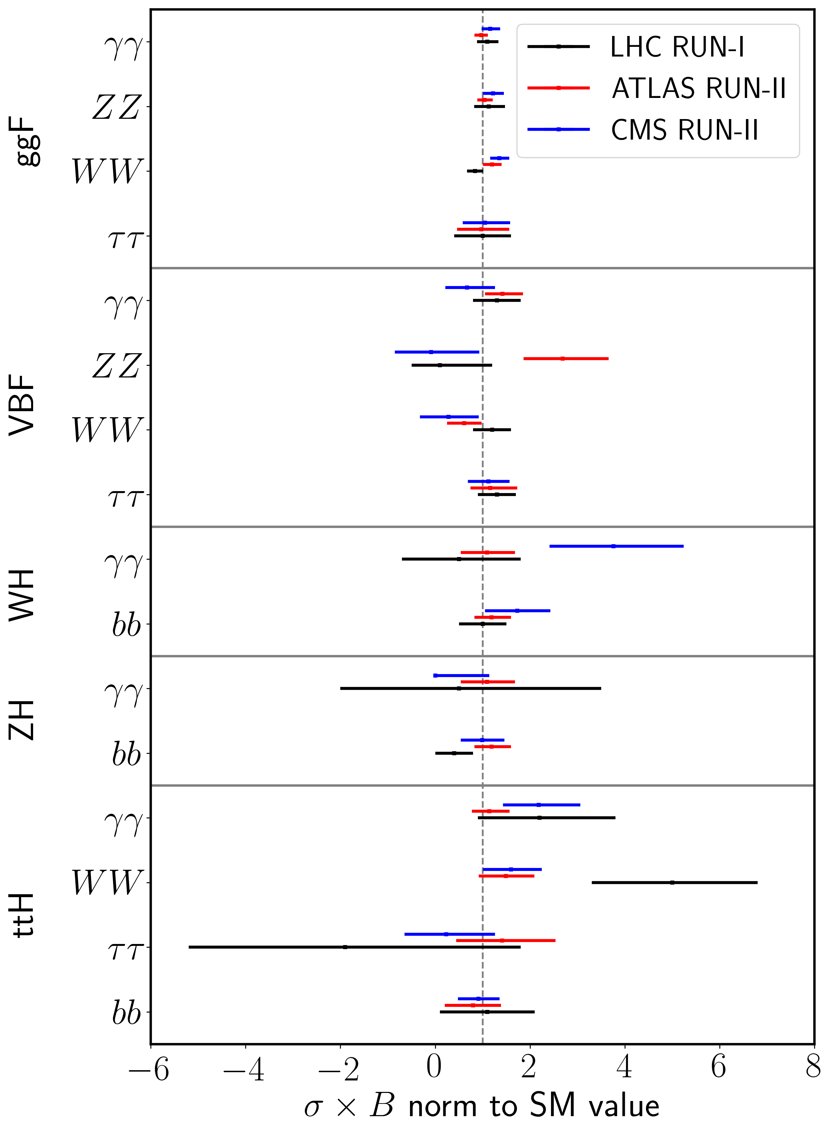
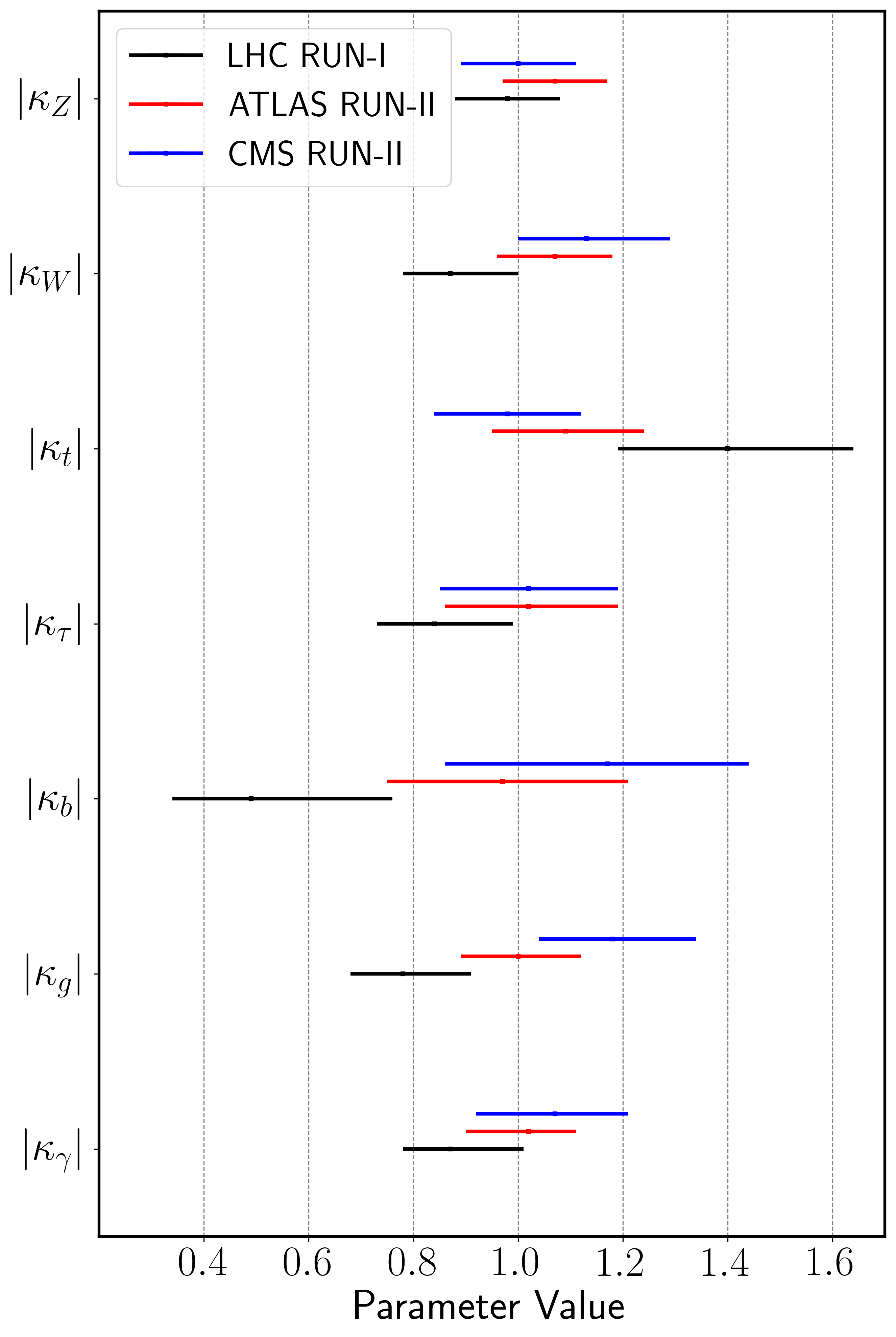
Figure 1: Current Higgs signal strength measurements for various channels (left) and the constraints on the $\kappa$ of different couplings assuming no additional BSM channel for the Higgs (right). Data is retrieved from Khachatryan:2016vau ; ATLAS-CONF-2018-031 ; Sirunyan:2018koj .

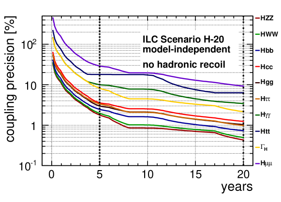
Figure 2: The precision on various couplings of the Higgs boson in scenario H-20. Figure is getting from Barklow:2015tja .

The measurements can be significantly improved with the proposed Higgs factories. As an example, the H-20 scenario of ILC Barklow:2015tja will accumulate about 4000 fb^-1 at $\sqrt{s}=$500 GeV, 200 fb^-1 at $\sqrt{s}=$350 GeV and 2000 fb^-1 at $\sqrt{s}=$250 GeV. The detailed precisions of the signal strength measurements for different channels and $\sqrt{s}$ are listed in Tab. 1. Correspondingly, the coupling measurements can be improved considerably as shown in Fig. 2. With the huge data accumulated in the Higgs factories, sub-percent precision can be expected for the measurement of the Higgs couplings which will in turn put stringent constraints on new physics.

collider	ILC
$\sqrt{s}$	250 GeV	350 GeV		500 GeV
$\int{\mathcal{L}}dt$	$\text{2 ab}^{-1}$	$\text{200 fb}^{-1}$		$\text{4 ab}^{-1}$
production	$Zh$	$Zh$	$\nu\bar{\nu}h$	$Zh$	$\nu\bar{\nu}h$	$t\bar{t}h$
$\Delta\sigma/\sigma$	0.71%	2.1%	$-$	1.06	$-$	$-$
decay	$\Delta(\sigma\cdot BR)/(\sigma\cdot BR)$
$h\to b\bar{b}$	0.42%	1.67%	1.67%	0.64%	0.25%	9.9%
$h\to c\bar{c}$	2.9%	12.7%	16.7%	4.5%	2.2%	$-$
$h\to gg$	2.5%	9.4%	11.0%	3.9%	1.5%	$-$
$h\to WW^{*}$	1.1%	8.7%	6.4%	3.3%	0.85%	$-$
$h\to\tau^{+}\tau^{-}$	2.3%	4.5%	24.4%	1.9%	3.2%	$-$
$h\to ZZ^{*}$	6.7%	28.3%	21.8%	8.8%	2.9%	$-$
$h\to\gamma\gamma$	12.0%	43.7%	50.1%	12.0%	6.7%	$-$
$h\to\mu^{+}\mu^{-}$	25.5%	97.6%	179.8%	31.1%	25.5%	$-$

Table 1: Estimated statistical precisions for Higgs measurements obtained at the ILC with various center-of-mass energies Barklow:2015tja .

2.2 Electroweak Measurement

Beside Higgs related measurements, the proposed Higgs factories will also have their own Z-pole measurement. The current best precision measurements for Z-pole physics mostly come from the LEP-I as well as Tevatron and the LHC Baak:2014ora ; Haller:2018nnx . These measurements will be significantly improved at future lepton colliders CEPC-SPPCStudyGroup:2015csa ; Gomez-Ceballos:2013zzn ; fccpara ; fccplan ; Asner:2013psa . The anticipated precisions on several measurements for Z-pole program are listed in Tab. 2.

Given the complexity of a full Z-pole precision global fit, we instead use the Peskin-Takeuchi oblique parameters S, T and U Peskin:1991sw to present the implications of the Z-pole precision. Corresponding to the precision listed in Tab. 2, the constrained S, T and U ranges and associated error correlation matrix are listed in Tab. 3, which are obtained by using Gfitter package Baak:2014ora .

	ILC Precision
$\alpha_{s}(M_{Z}^{2})$	$\pm 1.0\times 10^{-4}$
$\Delta\alpha_{\rm had}^{(5)}(M_{Z}^{2})$	$\pm 4.7\times 10^{-5}$
$m_{Z}$ [GeV]	$\pm 0.0021$
$m_{t}$ [GeV] (pole)	$\pm 0.03_{\rm exp}\pm 0.1_{\rm th}$
$m_{h}$ [GeV]	$<\pm 0.1$
$m_{W}$ [GeV]	$\left(\pm 5_{\rm exp}\pm 1_{\rm th}\right)\times 10^{-3}$
$\sin^{2}\theta^{\ell}_{\rm eff}$	$\left(\pm 1.3_{\rm exp}\pm 1.5_{\rm th}\right)\times 10^{-5}$
$\Gamma_{Z}$ [GeV]	$\pm 0.001$

Table 2: Anticipated precisions of the EW observables at the future lepton colliders. The results are mainly from Fan:2014vta ; Lepage:2014fla ; Baak:2013fwa ; Baak:2014ora ; LiangTalk .

	Current ($1.7\times 10^{7}\ Z$’s)				ILC ($10^{9}Z$’s)
	$\sigma$	correlation			$\sigma$	correlation
		$S$	$T$	$U$	($10^{-2}$)	$S$	$T$	$U$
$S$	$0.04\pm 0.11$	1	0.92	$-0.68$	$3.53$	1	0.988	$-0.879$
$T$	$0.09\pm 0.14$	$-$	1	$-0.87$	$4.89$	$-$	1	$-0.909$
$U$	$-0.02\pm 0.11$	$-$	$-$	1	$3.76$	$-$	$-$	1

Table 3: Estimated $S$, $T$, and $U$ ranges and correlation matrices $\rho_{ij}$ from $Z$-pole precision measurements of the current results, mostly from LEP-I ALEPH:2005ab , and at future lepton colliders ILC  Asner:2013psa . Gfitter package Baak:2014ora is used in obtaining those constraints.

3 Type-II 2HDM

3.1 Model Setup

In 2HDM, two $SU(2)_{L}$ scalar doublets $\Phi_{i}$ ($i=1,2$) with a hyper-charge assignment $Y=+1/2$:

$$\Phi_{i}=\left(\begin{array}[]{c}\phi_{i}^{+}\\ \frac{v_{i}+\phi_{i}^{0}+iG_{i}}{\sqrt{2}}\end{array}\right)$$ (5)

The neutral component of each doublet obtains a vacuum expectation value (vev) $v_{i}$ (i=1,2) after EWSB satisfying $v_{1}^{2}+v_{2}^{2}=v^{2}=(246\text{ GeV})^{2}$, and $v_{2}/v_{1}=\tan\beta$.

The 2HDM Lagrangian for the Higgs sector can be written as

$$\mathcal{L}=\sum_{i}|D_{\mu}\Phi_{i}|^{2}-V(\Phi_{1},\Phi_{2})+\mathcal{L}_{\text{Yuk}},$$ (6)

where the Higgs potential has following form:

$$V(\Phi_{1},\Phi_{2})= m_{11}^{2}\Phi_{1}^{\dagger}\Phi_{1}+m_{22}^{2}\Phi_{2}^{\dagger}\Phi_{2}-m_{12}^{2}(\Phi_{1}^{\dagger}\Phi_{2}+h.c.)+\frac{\lambda_{1}}{2}(\Phi_{1}^{\dagger}\Phi_{1})^{2}+\frac{\lambda_{2}}{2}(\Phi_{2}^{\dagger}\Phi_{2})^{2}$$

$$\lambda_{3}(\Phi_{1}^{\dagger}\Phi_{1})(\Phi_{2}^{\dagger}\Phi_{2})+\lambda_{4}(\Phi_{1}^{\dagger}\Phi_{2})(\Phi_{2}^{2}\Phi_{1})+\frac{1}{2}\lambda_{5}\left[(\Phi_{1}^{\dagger}\Phi_{2})^{2}+h.c.\right]$$ (7)

where we assume the conservation of CP symmetry.

In general, there are four types Yukawa couplings assigning different doublet to different type fermions. In this work, we focus on Type-II of which the Yukawa couplings is:

$$-\mathcal{L}_{\text{Yuk}}=Y_{d}\bar{Q}_{L}\Phi_{1}d_{R}+Y_{e}\bar{L}_{L}\Phi_{1}e_{R}+Y_{u}\bar{Q}_{L}i\sigma_{2}\Phi_{2}^{*}u_{R}+h.c.$$ (8)

After EWSB, three of the degree of freedom in two doublets are eaten by the SM gauge bosons, providing their masses. The remaining physical mass eigenstates are two CP-even neutral Higgs bosons $h$ and $H$, one CP-odd neutral Higgs boson $A$, and a pair of charged scalars $H^{\pm}$. Instead of the eight parameters in the potential $m_{11}^{2}$, $m_{22}^{2}$, $m_{12}^{2}$, $\lambda_{1,2,3,4,5}$, more physical parameters will be used: ($v$, $\tan\beta$, $\alpha$, $m_{h}$, $m_{H}$, $m_{A}$, $m_{H^{\pm}}$, $m_{12}^{2}$).

In term of these mass eigenstates, the effective Lagrangian for the couplings between these scalars and SM particles is

$$\mathcal{L} =\kappa_{Z}\frac{m_{Z}^{2}}{v}Z_{\mu}Z^{\mu}h+\kappa_{W}\frac{2m_{W}^{2}}{v}W_{\mu}^{+}W^{\mu-}h+\kappa_{g}\frac{\alpha_{s}}{12\pi v}G_{\mu\nu}^{a}G^{a\mu\nu}h+\kappa_{\gamma}\frac{\alpha}{2\pi v}A_{\mu\nu}A^{\mu\nu}h$$

$$+\kappa_{Z\gamma}\frac{\alpha}{\pi v}A_{\mu\nu}Z^{\mu\nu}h-\left(\kappa_{u}\sum_{u}\frac{m_{f}}{v}\bar{f}f+\kappa_{d}\sum_{d}\frac{m_{f}}{v}\bar{f}f+\kappa_{\ell}\sum_{\ell}\frac{m_{f}}{v}\bar{f}f\right)h$$ (9)

where, at tree level, we have

$$\kappa_{Z}=\kappa_{W}=\sin(\beta-\alpha),\quad\kappa_{u}=\frac{\cos\alpha}{\sin\beta},\quad\kappa_{d,\ell}=-\frac{\sin\alpha}{\cos\beta}.$$ (10)

Note that $\kappa_{g}$, $\kappa_{\gamma}$ and $\kappa_{Z\gamma}$ are generated at one-loop. From above $\kappa$’s, the alignment limit can be identified as $\cos(\beta-\alpha)=0$.

It is also important to have a discussion for the triple couplings among scalars. At the alignment limit, we have

$$\lambda_{h\Phi\Phi}=-\frac{C_{\Phi}}{2v}(m_{h}^{2}+2m_{\Phi}^{2}-\frac{2m_{12}^{2}}{\sin\beta\cos\beta}).$$ (11)

with $C_{\Phi}=2(1)$ for $\Phi=H^{\pm}(H,A)$. With degenerate masses $m_{\Phi}\equiv m_{H}=m_{A}=m_{H^{\pm}}$, we introduce a new parameter $\lambda$ as

$$\lambda v^{2}\equiv m_{\Phi}^{2}-\frac{m_{12}^{2}}{\sin\beta\cos\beta},$$ (12)

which is the parameter that enters the Higgs self-couplings and relevant for the loop corrections to the SM-like Higgs boson couplings. This parameter could be used interchangeably with $m_{12}^{2}$. For the rest of our analysis, $v=246$ GeV and $m_{h}=125$ GeV are used. The remaining free parameters are

$$\tan\beta,\cos(\beta-\alpha),m_{H},m_{A},m_{H^{\pm}},\lambda$$ (13)

3.2 Loop corrections to Higgs couplings

We define the normalized SM-like Higgs boson couplings including loop effects as

$$\kappa_{\text{loop}}^{\text{2HDM}}\equiv\frac{g_{\rm tree}^{\rm 2HDM}+g_{\rm loop}^{\rm 2HDM}}{g_{\rm tree}^{\rm SM}+g_{\rm loop}^{\rm SM}}$$ (14)

In our calculations, we adopt the on-shell renormalization scheme FeynArts-SM . The conventions for the renormalization constants and the renormalization conditions are mostly following Refs. FeynArts-SM ; Kanemura:2004mg . All related counter terms, renormalization constants and renormalization conditions are implemented according to the on-shell scheme and incorporated into model files of FeynArts Hahn:2000kx . One-loop corrections are generated using FeynArts and FormCalc Hahn:2016ebn including all possible one-loop diagrams. FeynCalc Shtabovenko:2016sxi ; Mertig:1990an is also used to simplify the analytical expressions. LoopTool Hahn:1998yk is used to evaluate the numerical value of all the loop-induced amplitude. The numerical results have been cross-checked with another numerical program H-COUP Kanemura:2017gbi in some cases.

Further, the 2HDM contributions to the oblique parameters are given by He:2001tp :

$$\Delta\,S = \frac{1}{\pi\,m_{Z}^{2}}\Big{\{}\Big{[}{\cal B}_{22}(m_{Z}^{2}\,;m_{H}^{2}\,,m_{A}^{2})-{\cal B}_{22}(m_{Z}^{2}\,;m_{H^{\pm}}^{2}\,,m_{H^{\pm}}^{2})\Big{]}$$ (15)

$$+\Big{[}{\cal B}_{22}(m_{Z}^{2}\,;m_{h}^{2}\,,m_{A}^{2})-{\cal B}_{22}(m_{Z}^{2}\,;m_{H}^{2}\,,m_{A}^{2})+{\cal B}_{22}(m_{Z}^{2}\,;m_{Z}^{2}\,,m_{H}^{2})-{\cal B}_{22}(m_{Z}^{2}\,;m_{Z}^{2}\,,m_{h}^{2})$$

$$-m_{Z}^{2}{\cal B}_{0}(m_{Z}\,;m_{Z}\,,m_{H}^{2})+m_{Z}^{2}{\cal B}_{0}(m_{Z}\,;m_{Z}\,,m_{h}^{2})\Big{]}\cos^{2}(\beta-\alpha)\Big{\}}\,,$$

$$\Delta T = \frac{1}{16\pi\,m_{W}^{2}\,s_{W}^{2}}\Big{\{}\Big{[}F(m_{H^{\pm}}^{2}\,,m_{A}^{2})+F(m_{H^{\pm}}^{2}\,,m_{H}^{2})-F(m_{A}^{2}\,,m_{H}^{2})\Big{]}$$ (16)

$$+\Big{[}F(m_{H^{\pm}}^{2}\,,m_{h}^{2})-F(m_{H^{\pm}}^{2}\,,m_{H}^{2})-F(m_{A}^{2}\,,m_{h}^{2})+F(m_{A}^{2}\,,m_{H}^{2})$$

$$+F(m_{W}^{2}\,,m_{H}^{2})-F(m_{W}^{2}\,,m_{h}^{2})-F(m_{Z}^{2}\,,m_{H}^{2})+F(m_{Z}^{2}\,,m_{h}^{2})$$

$$+4m_{Z}^{2}\overline{B}_{0}(m_{Z}^{2}\,,m_{H}^{2}\,,m_{h}^{2})-4m_{W}^{2}\overline{B}_{0}(m_{W}^{2}\,,m_{H}^{2}\,,m_{h}^{2})\Big{]}\cos^{2}(\beta-\alpha)\Big{\}}\,,$$

$$\Delta\,U = -\Delta\,S+\frac{1}{\pi m_{W}^{2}}\Big{\{}\Big{[}{\cal B}_{22}(m_{W}^{2},m_{A}^{2},m_{H^{\pm}}^{2})-2{\cal B}_{22}(m_{W}^{2},m_{H^{\pm}}^{2},m_{H^{\pm}}^{2})+{\cal B}_{22}(m_{W}^{2},m_{H}^{2},m_{H^{\pm}}^{2})\Big{]}$$ (17)

$$+\Big{[}{\cal B}_{22}(m_{W}^{2},m_{h}^{2},m_{H^{\pm}}^{2})-{\cal B}_{22}(m_{W}^{2},m_{H}^{2},m_{H^{\pm}}^{2})+{\cal B}_{22}(m_{W}^{2},m_{W}^{2},m_{H}^{2})-{\cal B}_{22}(m_{W}^{2},m_{W}^{2},m_{h}^{2})$$

$$-m_{W}^{2}{\cal B}_{0}(m_{W}^{2},m_{W}^{2},m_{H}^{2})+m_{W}^{2}{\cal B}_{0}(m_{W}^{2},m_{W}^{2},m_{h}^{2})\Big{]}\cos^{2}(\beta-\alpha)\Big{\}}\,,$$

4 Global Fitting

In our analysis, global fit is performed to get the constraints on the model parameters by constructing the $\chi^{2}$ with the profile likelihood method

$$\chi^{2}=\sum_{i}\frac{(\mu_{i}^{\text{BSM}}-\mu_{i}^{\text{obs}})^{2}}{\sigma_{\mu_{i}}^{2}},$$ (18)

where $\mu_{i}^{\text{BSM}}=\frac{(\sigma\times{\rm BR})_{\text{BSM}}}{(\sigma\times{\rm BR})_{\text{SM}}}$, and $i$ runs over all available channels, the corresponding errors $\sigma_{\mu_{i}}$ for all these channels are listed in Tab. 1.

We also incorporate the Z-pole precision measurements by fitting into the oblique parameters $S$, $T$ and $U$ of which the $\chi^{2}$ reads

$$\chi^{2}=\sum_{ij}(X_{i}-\hat{X}_{i})(V^{-1})_{ij}(X_{j}-\hat{X}_{j}),$$ (19)

with $X_{i}=(\Delta S,\Delta T,\Delta U)_{\text{2HDM}}$ being the predicted values in 2HDM, while $\hat{X}_{i}=(\Delta S,\Delta T,\Delta U)$ being the best-fit central value (assuming 0 for future measurements). $V$ is the covariance matrix with $V_{ij}=\sigma_{i}\rho_{ij}\sigma_{j}$. The corresponding errors $\sigma_{i}$ and the correlation matrix $\rho_{ij}$ are listed in Tab. 3 for both current measurement and ILC prospects.

At tree level, the Higgs couplings only involve $\tan\beta$ and $\cos(\beta-\alpha)$. Hence, from Higgs measurement, we can only constraint the parameter space in $\tan\beta$ vs. $\cos(\beta-\alpha)$ plane. The results from ATLAS ATLAS-CONF-2018-031 and CMS Sirunyan:2018koj are shown in Fig. 3. Beside the extra arm corresponding to the wrong sign scenario, the current measurement strongly constrain the range of $\cos(\beta-\alpha)$. This can be further improved by the Higgs measurement at the ILC which can be seen in Fig. 4. From the fitting results, at tree level, we can already constrain the $\cos(\beta-\alpha)$ to be at least less than 0.01.

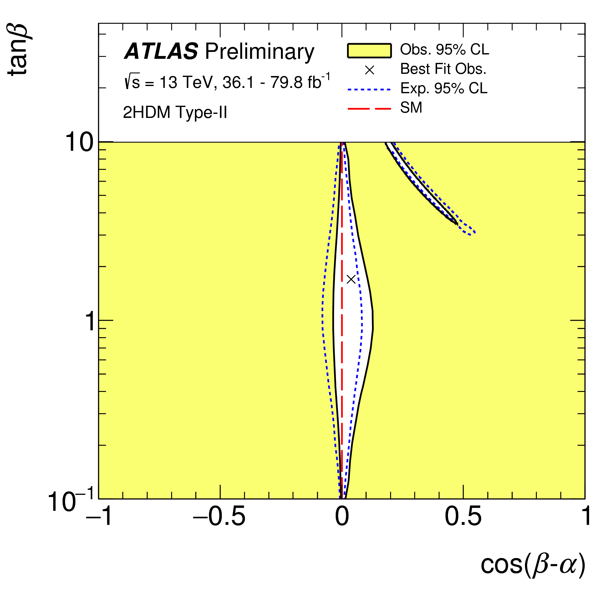
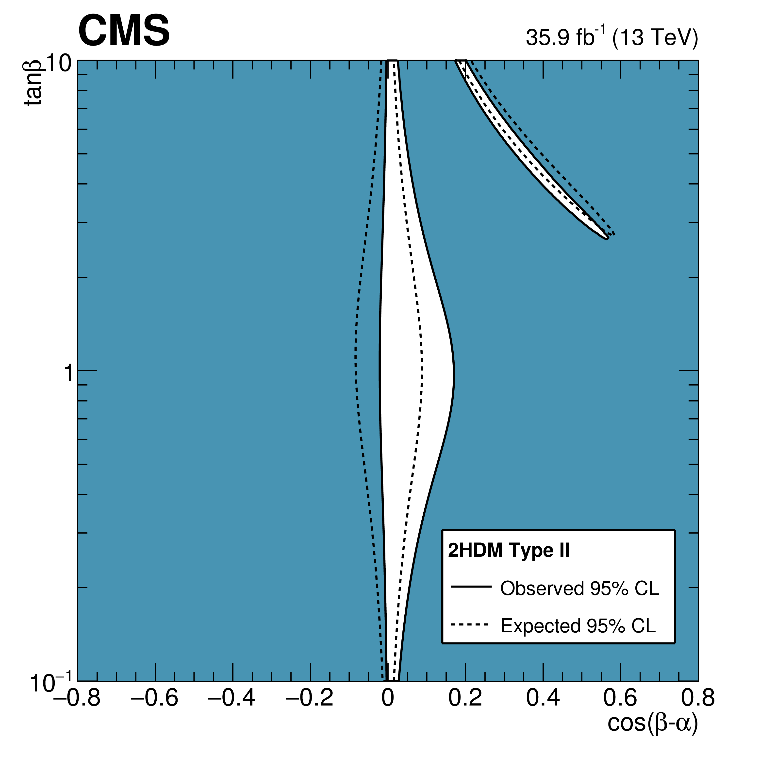
Figure 3: Current constraints from ATLAS (left) and CMS (right) for the Type-II 2HDM in $\tan\beta$ vs. $\cos(\beta-\alpha)$ plane. Figures are getting from ATLAS-CONF-2018-031 ; Sirunyan:2018koj .

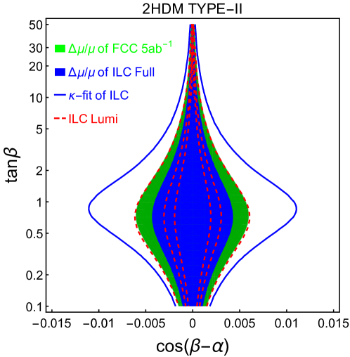
Figure 4: The prospected constraints from ILC measurement for the Type-II 2HDM in $\tan\beta$ vs. $\cos(\beta-\alpha)$ plane.

Using $hZZ$ coupling as example, at tree level, the couplings is

$$\mathcal{L}_{hZZ}=\frac{m_{Z}^{2}}{v}s_{\beta-\alpha}hZ_{\mu}Z^{\mu}\approx\left(1-\frac{1}{2}c_{\beta-\alpha}^{2}\right)\frac{m_{Z}^{2}}{v}hZ_{\mu}Z^{\mu}.$$ (20)

Hence, the deviation from the SM value is $\frac{1}{2}c_{\beta-\alpha}^{2}\frac{m_{Z}^{2}}{v}$. With the constraints from the ILC prospect, the coupling deviation is at about $\mathcal{O}(10^{-4})$ level. In this case, the loop induced correction which is not vanished even in the alignment limit can not be ignored any more. Further, including loop correction which has heavy scalars running in the loop also provides the possibility to constrain the mass of heavy scalars as well as the triple scalar couplings. With this consideration, we will consider three cases in sequence:

• Tree-level alignment + Mass degenerate:

  • $\cos(\beta-\alpha)=0$, $m_{\Phi}\equiv m_{H}=m_{A}=m_{H^{\pm}}$.

• Non-alignment + Mass degenerate:

  • $\cos(\beta-\alpha)\neq 0$, $m_{\Phi}\equiv m_{H}=m_{A}=m_{H^{\pm}}$.

• Non-alignment + Non-degenerate:

  • $\cos(\beta-\alpha)\neq 0$, $\Delta m_{A}=m_{A}-m_{H}$, $\Delta m_{C}=m_{H^{\pm}}-m_{H}$.

4.1 Alignment and Mass Degenerate Case

The first case we consider is when $\cos(\beta-\alpha)=0$ and all the heavy scalars are degenerate in mass. In this case, the free parameters are $\tan\beta$, $m_{\Phi}$ and $\lambda$. The corresponding exclusion results are shown in Fig. 5 where lines with different colors represent the exclusions for different choice of $\lambda$ in $m_{\Phi}$-$\tan\beta$ plane. The region to the right of the lines and the upper left region are allowed. From this figure, we can see that when the triple scalar coupling is not strong, we still have large allowed region as shown by the red and blue curves. The gaps around 350 GeV come from the top-pair threshold. When the triple scalar coupling is strong, the exclusion curves provide lower limits on the heavy scalar mass which is consistent with our prospects. For $\sqrt{\lambda v^{2}}=300$ GeV, a lower limit of 500 GeV on the mass is expected, while for $\sqrt{\lambda v^{2}}=500$ GeV, the heavy scalar mass should be larger than 1200 GeV.

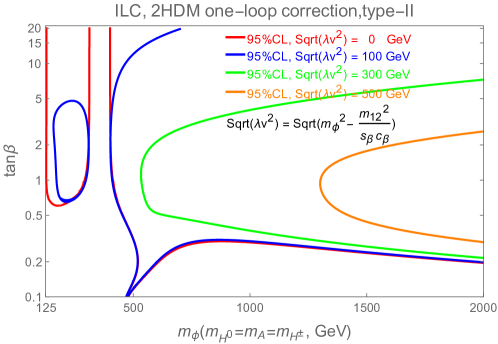
Figure 5: The exclusion line from Higgs measurement in the $m_{\Phi}$-$\tan\beta$ plane for different choice of $\lambda$

4.2 Non-alignment and Mass Degenerate Case

The second case we consider is when we deviate from the alignment limit but still assume that all heavy scalars are degenerated. In this case, the free parameters are $\tan\beta$, $\cos(\beta-\alpha)$, $m_{\Phi}$ and $\lambda$. We first show the result in Fig. 6 in the $m_{\Phi}$-$\tan\beta$ plane for different choice of $\cos(\beta-\alpha)$ (represented by lines with different colors) and of $\sqrt{\lambda v^{2}}$ (left panel: $\sqrt{\lambda v^{2}}=0$ GeV and right panel: $\sqrt{\lambda v^{2}}=300$ GeV). The constraints on other parameters are similar to the previous case, while it also shows different exclusion patterns for negative and positive choice of $\cos(\beta-\alpha)$. Note that, for the tree-level only results, Fig. 4, the constraints is symmetric for $\cos(\beta-\alpha)$. This shows the importance of the interference between loop corrections and the tree level couplings.

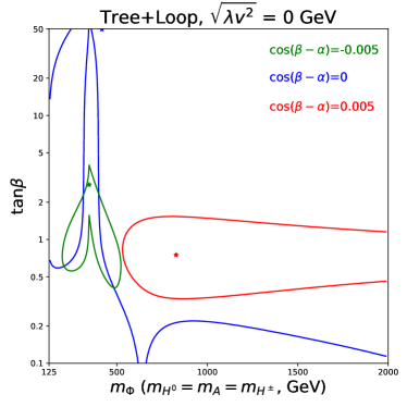
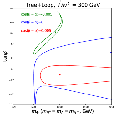
Figure 6: The exclusion lines for different choice of $\cos(\beta-\alpha)$ in $m_{\Phi}$-$\tan\beta$ plane, the left panel is for $\sqrt{\lambda v^{2}}=0$ GeV while the right panel is for $\sqrt{\lambda v^{2}}=300$ GeV.

To make this more clearer, we show the results in the $\cos(\beta-\alpha)$-$\tan\beta$ plane in Fig. 7. In the left panel, $\sqrt{\lambda v^{2}}=300$ GeV is fixed. The red region is the global fitting allowed region, while lines with different colors are the constraints from different couplings as indicated by the label. We can see that at large $\tan\beta$ region, the constraints from $\kappa_{\tau}$ and $\kappa_{b}$ push the allowed region away from the tree level results. At low $\tan\beta$ region, the allowed region is cut off by $\kappa_{c}$ and $\kappa_{g}$. Note that we are still in the degenerate cases, with this small $\cos(\beta-\alpha)$ we are probing, the constraint from $\kappa_{z}$ is rather weak as shown by the green line in the upper right corner. The effects of $\sqrt{\lambda v^{2}}$ is shown in the right panel of Fig. 7. We can see that the region will deviate from the tree level cases with increase of $\sqrt{\lambda v^{2}}$. Note that there is no more allowed region for larger value of $\sqrt{\lambda v^{2}}$ which put an upper limit on $\lambda$.

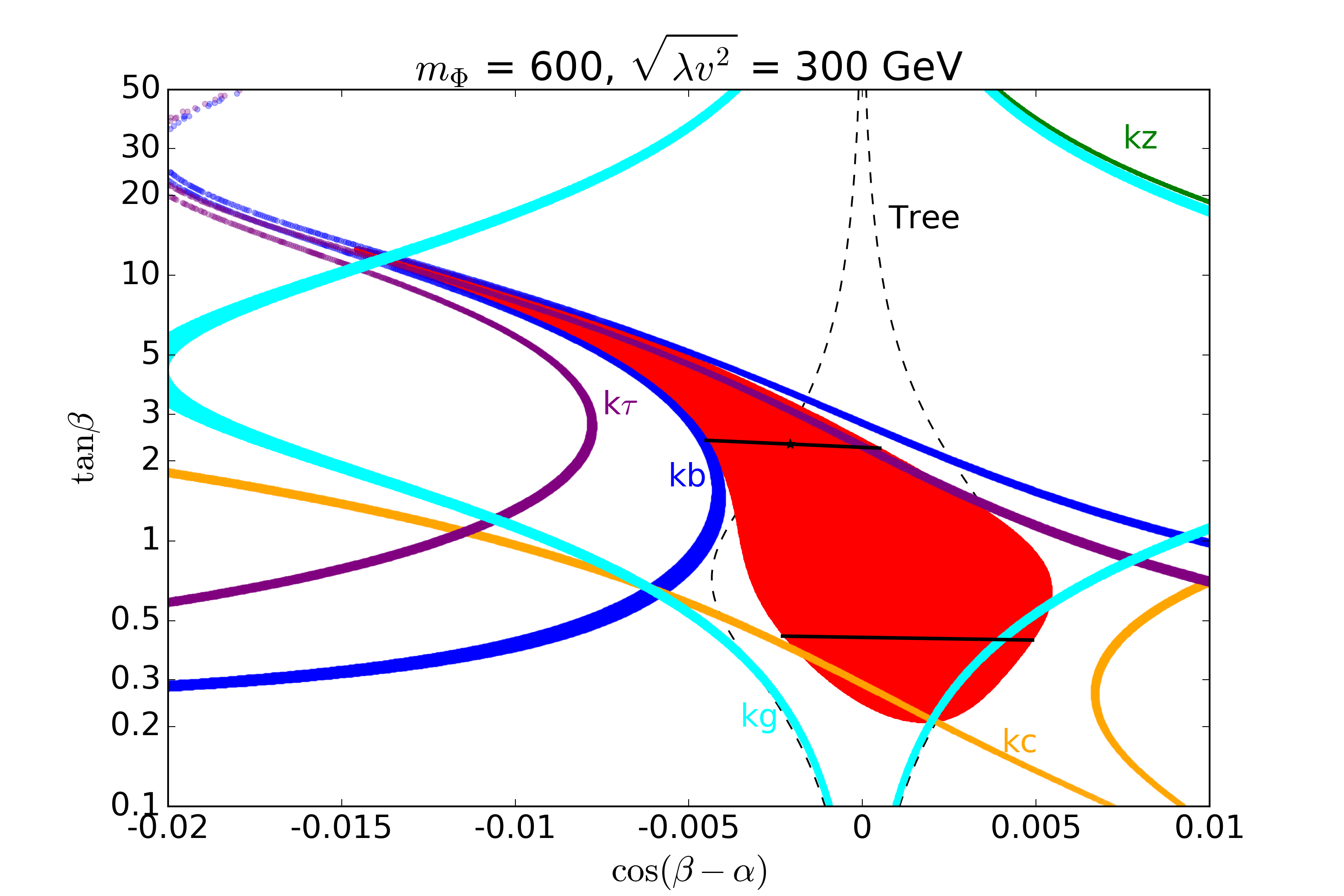
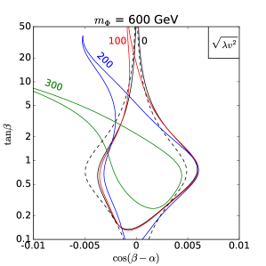
Figure 7: The exclusion lines in the $\cos(\beta-\alpha)$-$\tan\beta$ plane for $m_{\Phi}=600$ GeV. In the left panel, $\sqrt{\lambda v^{2}}=300$ GeV is fixed. The red region is the global fitting allowed region, while lines with different colors are the constraints from different couplings as indicated by the label. The black dashed line represents the tree level result. In the right panel, only the global fitting allowed regions are shown for different choice of $\sqrt{\lambda v^{2}}$.

4.3 Non-alignment and Non-degenerate Case

The last case we consider is the most general one. We allow both the deviation from the alignment and also the mass splittings. The new free parameters are the mass splittings among different scalars: $\Delta m_{A}=m_{A}-m_{H}$, $\Delta m_{C}=m_{H^{\pm}}-m_{H}$. The constraints on other parameters are similar to previous case. Hence, we focus on the constraints on mass differences here. When allowing mass splitting, the Z-pole measurements will also provide stringent constraints. The constraints from the T parameter is shown in Fig. 8 in $m_{A}$-$m_{C}$ plane. From this plot we can see that the Z-pole measurement has already put a strong constraint on the mass difference. Hence, a natural question would be whether the Higgs measurement can provide further information on the mass difference.

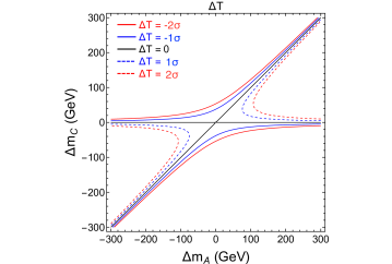
Figure 8: The constraints from T-parameter in $m_{A}$-$m_{C}$ plane. The blue and red lines represent the 1-$\sigma$ and 2-$\sigma$ region respectively.

The results from the Higgs measurement are shown in Fig. 9. In the left column, the individual constraints from Higgs measurement (solid lines) and Z-pole measurement (dashed line) are shown. We can see that both Higgs measurement and Z-pole measurement can constrain the mass splitting, while these two constraints are mis-aligned. Furthermore, the Higgs measurement is quite sensitive to the value of $\cos(\beta-\alpha)$. However, the T parameter constraints here merely changes for the range of the $\cos(\beta-\alpha)$ we considered here. When combining these, the allowed region is further shrunk as shown in the right column of Fig. 9. This result clearly shows the complementarity between the Higgs measurement and Z-pole measurement. For $\cos(\beta-\alpha)=0$ (blue lines), increasing the mass of the heavy scalar leads to larger allowed region which is consistent with the decoupling limit. However, when we deviate from $\cos(\beta-\alpha)=0$ ($\pm 0.007$ as shown by red and green lines in the plots), the allowed the region is even smaller for larger mass. This is due to the fact that when we approach decoupling limit, the parameter space will also be pushed into alignment limits, otherwise we suffer from either the unitarity/perturbativity problem or large correction induced by triple scalar couplings.

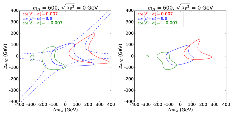
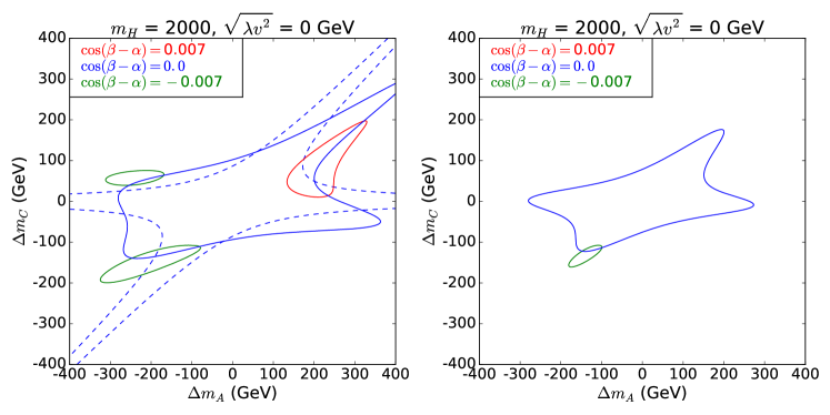
Figure 9: The constraints from Higgs measurement (left column) and Higgs measurement combined with Z-pole measurement (right column) in $\Delta m_{A}$-$\Delta m_{C}$ plane. The mass are set by $m_{H}=600$ and 2000 GeV for upper two and lower two panels respectively. Lines with different colors are for different choices of $\cos(\beta-\alpha)$ as indicated in the legend. The dashed contours in the left column are the Z-pole constraints which barely changes with $\cos(\beta-\alpha)$ in this range.

5 Summary

In this paper, we examined the impacts of the precision measurements of the SM parameters at the proposed Higgs factories using Type-II 2HDM as an example. At tree level, the current measurement has already push the model into the alignment limit region. The proposed Higgs factories can do even better with clean background. In this region, for some coupling, the loop corrections can not be ignored any more. When including loop induced contributions, we can further set bounds on the heavy scalar masses as well as the mass splitting. The triple scalar couping is constrained as well. In this sense, the Higgs precision measurement is complementary to the Z-pole measurement. The combination of these two kinds measurements can certainly provide more information about the new physics.

- (1) G. F. Giudice, Naturally Speaking: The Naturalness Criterion and Physics at the LHC, arXiv:0801.2562.
- (2) G. C. Branco, P. M. Ferreira, L. Lavoura, M. N. Rebelo, M. Sher, and J. P. Silva, Theory and phenomenology of two-Higgs-doublet models, Phys. Rept. 516 (2012) 1–102, [arXiv:1106.0034].
- (3) CEPC-SPPC Study Group, “CEPC-SPPC Preliminary Conceptual Design Report. 1. Physics and Detector.” http://cepc.ihep.ac.cn/preCDR/volume.html, 2015.
- (4) CEPC Study Group Collaboration, CEPC Conceptual Design Report: Volume 2 - Physics & Detector, arXiv:1811.10545.
- (5) H. Baer, T. Barklow, K. Fujii, Y. Gao, A. Hoang, S. Kanemura, J. List, H. E. Logan, A. Nomerotski, M. Perelstein, et al., The International Linear Collider Technical Design Report - Volume 2: Physics, arXiv:1306.6352.
- (6) TLEP Design Study Working Group Collaboration, M. Bicer et al., First Look at the Physics Case of TLEP, JHEP 01 (2014) 164, [arXiv:1308.6176].
- (7) “The FCC-ee design study.” http://tlep.web.cern.ch/content/fcc-ee-tlep.
- (8) M. Benedikt and F. Zimmermann, “Future Circular Collider Study, Status and Progress.” https://indico.cern.ch/event/550509/contributions/2413230/attachments/1396002/2128079/170116-MBE-FCC-Study-Status_ap.pdf, 2017.
- (9) N. Chen, T. Han, S. Su, W. Su, and Y. Wu, Type-II 2HDM under the Precision Measurements at the -pole and a Higgs Factory, arXiv:1808.02037.
- (10) ATLAS, CMS Collaboration, G. Aad et al., Measurements of the Higgs boson production and decay rates and constraints on its couplings from a combined ATLAS and CMS analysis of the LHC pp collision data at and 8 TeV, JHEP 08 (2016) 045, [arXiv:1606.02266].
- (11) CMS Collaboration, A. M. Sirunyan et al., Combined measurements of Higgs boson couplings in proton-proton collisions at 13 TeV, Submitted to: Eur. Phys. J. (2018) [arXiv:1809.10733].
- (12) ATLAS Collaboration Collaboration, Combined measurements of Higgs boson production and decay using up to 80 fb-1 of proton–proton collision data at 13 TeV collected with the ATLAS experiment, Tech. Rep. ATLAS-CONF-2018-031, CERN, Geneva, Jul, 2018.
- (13) T. Barklow, J. Brau, K. Fujii, J. Gao, J. List, N. Walker, and K. Yokoya, ILC Operating Scenarios, arXiv:1506.07830.
- (14) Gfitter Group Collaboration, M. Baak, J. Cúth, J. Haller, A. Hoecker, R. Kogler, K. Mönig, M. Schott, and J. Stelzer, The global electroweak fit at NNLO and prospects for the LHC and ILC, Eur. Phys. J. C74 (2014) 3046, [arXiv:1407.3792].
- (15) J. Haller, A. Hoecker, R. Kogler, K. Mönig, T. Peiffer, and J. Stelzer, Update of the global electroweak fit and constraints on two-Higgs-doublet models, arXiv:1803.01853.
- (16) D. M. Asner et al., ILC Higgs White Paper, in Proceedings, Community Summer Study 2013: Snowmass on the Mississippi (CSS2013): Minneapolis, MN, USA, July 29-August 6, 2013, 2013. arXiv:1310.0763.
- (17) M. E. Peskin and T. Takeuchi, Estimation of oblique electroweak corrections, Phys. Rev. D46 (1992) 381–409.
- (18) J. Fan, M. Reece, and L.-T. Wang, Possible Futures of Electroweak Precision: ILC, FCC-ee, and CEPC, JHEP 09 (2015) 196, [arXiv:1411.1054].
- (19) G. P. Lepage, P. B. Mackenzie, and M. E. Peskin, Expected Precision of Higgs Boson Partial Widths within the Standard Model, arXiv:1404.0319.
- (20) M. Baak et al., Working Group Report: Precision Study of Electroweak Interactions, in Proceedings, 2013 Community Summer Study on the Future of U.S. Particle Physics: Snowmass on the Mississippi (CSS2013): Minneapolis, MN, USA, July 29-August 6, 2013, 2013. arXiv:1310.6708.
- (21) Z. Liang, “Z and W Physics at CEPC.” http://indico.ihep.ac.cn/getFile.py/access?contribId=32&sessionId=2&resId=1&materialId=slides&confId=4338.
- (22) SLD Electroweak Group, DELPHI, ALEPH, SLD, SLD Heavy Flavour Group, OPAL, LEP Electroweak Working Group, L3 Collaboration, S. Schael et al., Precision electroweak measurements on the resonance, Phys. Rept. 427 (2006) 257–454, [hep-ex/0509008].
- (23) A. Denner, Techniques for calculation of electroweak radiative corrections at the one loop level and results for W physics at LEP-200, Fortsch. Phys. 41 (1993) 307–420, [arXiv:0709.1075].
- (24) S. Kanemura, Y. Okada, E. Senaha, and C. P. Yuan, Higgs coupling constants as a probe of new physics, Phys. Rev. D70 (2004) 115002, [hep-ph/0408364].
- (25) T. Hahn, Generating Feynman diagrams and amplitudes with FeynArts 3, Comput. Phys. Commun. 140 (2001) 418–431, [hep-ph/0012260].
- (26) A. Freitas and D. Stockinger, Gauge dependence and renormalization of tan beta in the MSSM, Phys. Rev. D66 (2002) 095014, [hep-ph/0205281].
- (27) M. Krause, R. Lorenz, M. Muhlleitner, R. Santos, and H. Ziesche, Gauge-independent Renormalization of the 2-Higgs-Doublet Model, JHEP 09 (2016) 143, [arXiv:1605.04853].
- (28) A. Denner, L. Jenniches, J.-N. Lang, and C. Sturm, Gauge-independent renormalization in the 2HDM, JHEP 09 (2016) 115, [arXiv:1607.07352].
- (29) L. Altenkamp, S. Dittmaier, and H. Rzehak, Renormalization schemes for the Two-Higgs-Doublet Model and applications to fermions, JHEP 09 (2017) 134, [arXiv:1704.02645].
- (30) S. Kanemura, M. Kikuchi, K. Sakurai, and K. Yagyu, Gauge invariant one-loop corrections to Higgs boson couplings in non-minimal Higgs models, Phys. Rev. D96 (2017), no. 3 035014, [arXiv:1705.05399].
- (31) T. Hahn, S. Paßehr, and C. Schappacher, FormCalc 9 and Extensions, PoS LL2016 (2016) 068, [arXiv:1604.04611]. [J. Phys. Conf. Ser.762,no.1,012065(2016)].
- (32) V. Shtabovenko, R. Mertig, and F. Orellana, New Developments in FeynCalc 9.0, Comput. Phys. Commun. 207 (2016) 432–444, [arXiv:1601.01167].
- (33) R. Mertig, M. Bohm, and A. Denner, FEYN CALC: Computer algebraic calculation of Feynman amplitudes, Comput. Phys. Commun. 64 (1991) 345–359.
- (34) T. Hahn and M. Perez-Victoria, Automatized one loop calculations in four-dimensions and D-dimensions, Comput. Phys. Commun. 118 (1999) 153–165, [hep-ph/9807565].
- (35) S. Kanemura, M. Kikuchi, K. Sakurai, and K. Yagyu, H-COUP: a program for one-loop corrected Higgs boson couplings in non-minimal Higgs sectors, arXiv:1710.04603.
- (36) H.-J. He, N. Polonsky, and S.-f. Su, Extra families, Higgs spectrum and oblique corrections, Phys. Rev. D64 (2001) 053004, [hep-ph/0102144].