Magnetic oscillations of in-plane conductivity in quasi-two-dimensional metals

Abstract

We develop the theory of transverse magnetoresistance in layered quasi-two-dimensional metals. Using the Kubo formula and harmonic expansion, we calculate intralayer conductivity in a magnetic field perpendicular to conducting layers. The analytical expressions for the amplitudes and phases of magnetic quantum oscillations (MQO) and of the so-called slow oscillations (SlO) are derived and applied to analyze their behavior as a function of several parameters: magnetic field strength, interlayer transfer integral and the Landau-level width. Both the MQO and SlO of intralayer and interlayer conductivities have approximately opposite phase in weak magnetic field and the same phase in strong field. The amplitude of SlO of intralayer conductivity changes sign at $\omega_{c}\tau_{0}=\sqrt{3}$. There are several other qualitative difference between magnetic oscillations of in-plane and out-of-plane conductivity. The results obtained are useful to analyze experimental data on magnetoresistance oscillations in various strongly anisotropic quasi-2D metals.

I Introduction

Magnetic quantum oscillations (MQO) is a powerful tool for studying electronic dispersion and Fermi surface geometry of metallic compoundsAbrik ; Ziman ; Shoenberg . Last decades it is actively used to investigate the electronic structure of strongly anisotropic layered compounds, including organic metals (see, e.g., Refs. [MarkReview2004, ; Singleton2000Review, ; OMRev, ; KartPeschReview, ; MQORev, ; LebedBook, ] for reviews), high-temperature superconductorsHusseyNature2003 ; ProustNature2007 ; SebastianNature2008 ; AudouardPRL2009 ; SingletonPRL2010 ; SebastianPNAS2010 ; SebastianPRB2010 ; SebastianPRL2012 ; SebastianNature2014 ; ProustNatureComm2015 (reviewed in Refs. [SebastianRepProgPhys2012, ; ProustComptesRendus2013, ; AnnuReviewYBCO2015, ]), etc. In layered compounds magnetoresistance has several new and useful qualitative effects, which do not appear in almost isotropic 3D metals. The theory of magnetoresistance in 2D metalsAndoFowlerSternRMP82 ; QHERMP1995 , extensively developed in connection to quantum Hall effect, is also inapplicable to quasi-2D (Q2D) metals even a weak interlayer hopping changes drastically the 2D localization effects and most electronic properties.

The Fermi surface (FS) of layered metals, e.g., corresponding to the electron dispersion in Eq. (3), is a warped cylinder. Such a FS has two close extremal cross-section areas $S_{1}$ and $S_{2}$ by the planes in $k$-space perpendicular to magnetic field $\bm{B}$, which give two close MQO frequencies $F_{1,2}=S_{1,2}/(2\pi e\hbar)$. According to the standard theoryAbrik ; Ziman ; Shoenberg , the observed MQO are given by the sum of oscillations with these two frequencies and almost equal amplitudes, which gives the beats of MQO amplitudeShoenberg , typical to Q2D metals. The beat frequency

$$\Delta F\equiv F_{1}-F_{2}\approx 2t_{z}B_{z}/(\hbar\omega_{c}),$$ (1)

can be used to measure the interlayer transfer integral $t_{z}\approx\Delta F\hbar\omega_{c}/(2B_{z})$, while its nontrivial dependence on the tilt angle $\theta$ of magnetic field (with respect to the normal to conducting layers), given byYam

$$\Delta F\left(\theta\right)/\Delta F\left(0\right)=J_{0}\left(k_{F}d\tan\theta\right),$$ (2)

allows to extract the in-plane Fermi momentum $k_{F}$. As follows from Eq. (2), the beat frequency $\Delta F\left(\theta\right)$ goes to zero in the so-called Yamaji angles $\theta_{Yam}$, given by the zeros of the Bessel function: $J_{0}\left(k_{F}d\tan\theta_{Yam}\right)=0$. The angular oscillations of the effective interlayer transfer integral $t_{z}\left(\theta\right)$, given by Eq. (2), also result in the angular magnetoresistance oscillations (AMRO), first discoveredKartsAMRO1988 in Q2D organic metal $\beta$-(BEDT-TTF)₂IBr₂ in 1988 and then actively studied both in Q2D and Q1D organic metalsMarkReview2004 ; Singleton2000Review ; OMRev ; KartPeschReview ; MQORev ; LebedBook ; Yagi1990 ; Kurihara ; MosesMcKenzie1999 ; TarasPRB2014 . The interplay between AMRO and MQO is also nontrivialTarasPRB2014 ; TarasPRB2017 and leads to some new effects, such as “false spin zeros”TarasPRB2017 .

Another interesting feature of magnetoresistance in Q2D metals is the so-called slow oscillations (SlO)SO ; Shub . These oscillations come from the mixing of two close frequencies $F_{1}$ and $F_{2}$ and have the frequency equal to the doubled beat frequency in Eq. (1). Similarly to AMRO and contrary to the usual MQO, the SlO are not sensitive to the smearing of the Fermi level, because they contain only the difference of Fermi levels at different $k_{z}$ given by $t_{z}$. Hence, the SlO are usually much stronger than the true MQO and can be observed at much higher temperatureSO ; GrigEuroPhys2016 . These slow oscillations were first observed in layered organic metal $\beta$-(BEDT-TTF)₂IBr₂ and erroneously interpreted as MQO from small FS pocketsKar1 ; Kar2 . Similar oscillations have also been observed in other organic conductors, e.g., $\beta$-(BEDT-TTF)₂I₃ Kar3 ; Wosn2 , $\kappa$-(BEDT-TTF)₂Cu₂(CN)₃ Ohmi , and $\kappa$-(BEDT-TSF)₂C(CN)₃ togo , while the band structure calculationsOMRev do not predict the corresponding small FS pockets in these compounds. The $k_{z}$ dispersion is not the only possible source of SlO. In fact, any splitting of the electron dispersion, leading to two close FS extremal cross-section areas, produces slow oscillations of MR with frequency given by the double difference between these FS areas. For example, the bilayer crystal structure, common in many cuprate high-Tc superconductors and in numerous other strongly anisotropic materials, produces such splitting of electron spectrum and the corresponding SlOGrigEuroPhys2016 ; MQOYBCOJETPL ; MQOYBCOPRB .

The SlO turn out to be quite useful to study the parameters of electronic structure of layered metals. First, their frequency $F_{SlO}=2\Delta F$ gives the difference between the two close extremal FS cross-section areas. Depending on the origin of SlO, this gives the strength of FS warping due to $k_{z}$ dispersion and the value of the interlayer transfer integral $t_{z}$ according to Eq. (1), the bilayer splitting or another type of splitting of electron spectrum. Second, the Dingle temperature $T_{D}^{\ast}$ of SlO is considerably less than the Dingle temperature $T_{D}$ of MQOSO , because at low temperature it only contains the contribution from short-range impurities and does not contain the variations of the Fermi level due to long-range spatial inhomogeneities that damp MQO. Hence, the comparison of the Dingle temperatures of SlO and MQO gives information about the type of disorder. In typical samples of organic metal $\beta$-(BEDT-TTF)₂I₃ the ratio $T_{D}/T_{D}^{\ast}\approx 5.3\gg 1$SO , which makes SlO much stronger than MQO at any temperature. Third, if SlO are due to $k_{z}$ dispersion, the angular dependence of SlO frequency gives the in-plane Fermi momentum $k_{F}$ according to Eq. (2).

In addition to SlO, in Q2D metals there is another notable effect of a phase shift of the beats of MQO of interlayer conductivity as compared to magnetizationPhSh . This phase shift increases with the increase of magnetic field. The explanation and calculation of this effectPhSh ; Shub , done using the Boltzmann transport equation and the Kubo formula, has shown that, similarly to SlO, it appears when the terms $\sim\hbar\omega_{c}/t_{z}$ are not neglected. Hence, in almost isotropic 3D metals, where $t_{z}$ is of the order of Fermi energy $E_{F}\gg\hbar\omega_{c}$, both effect are negligibly small. However, in Q2D conductors, where $\hbar\omega_{c}/t_{z}\sim 1$, both effects can be strong.

The rigorous theory of SlO was developed only for the interlayer magnetoresistanceSO ; Shub . However, their quite generic origin and various experimentsSebastianNature2008 ; ProustNatureComm2015 ; GrigEuroPhys2016 suggest that similar SlO must also be observed in the in-plane electronic transport. A semi-phenomenological description of in-plane SlO, proposed in Refs. [GrigEuroPhys2016, ; MQOYBCOPRB, ], does not contain the calculation of in-plane diffusion coefficient $D_{||}$ but only assumes that its oscillations have the same phase as the oscillations of the density of states (DoS) due to the Landau quantization. Even this is not generally valid, as we show below. In addition, in Refs. [GrigEuroPhys2016, ; MQOYBCOPRB, ; Korsh, ] the amplitude of MQO of $D_{||}$, which affects the amplitude and even the sign of SlO of intralayer MR, has not been calculated.

In this paper we calculate the in-plane MR in layered Q2D metals using the Feynman diagram technique. This calculation shows some qualitative differences of intralayer and interlayer MR. For example, the amplitude of SlO turns out to have non-monotonic magnetic-field dependence and may even change the sign. The phase shifts of MQO and their beats in Q2D metals also differ for intralayer and interlayer MR.

II The model and basic formulas

Let’s consider layered Q2D metals with electron dispersion

$$\epsilon_{3D}(\bm{k})=\hbar^{2}\left(k_{x}^{2}+k_{y}^{2}\right)/(2m_{\ast})-2t_{z}\cos(k_{z}d),$$ (3)

where the interlayer transfer integral $t_{z}$ is assumed to be independent of electron momentum. In a magnetic field $\bm{B}$ along the $z$-axis, i.e., perpendicular to conducting layers, its electron dispersion becomes

$$\epsilon(n,\,k_{z})=\hbar\omega_{c}\left(n+\frac{1}{2}\right)-2t_{z}\cos(k_{z}d),$$ (4)

where $\omega_{c}=eB_{z}/(m_{\ast}c)$ is cyclotron frequency, $m_{\ast}$ is effective electron mass, $e$ is the electric charge, and $c$ is the speed of light. The diagonal component of the in-plane conductivity tensor $\sigma_{ij}(\varepsilon)$ is given by Economou ; AGD ; Kurihara ; Streda ; Bastin

$$\sigma_{xx}(\varepsilon) = \frac{e^{2}\hbar}{\pi V}\sum_{\left\{n,\,n^{\prime}\right\}=0}^{+\infty}\sum_{k_{x},\,k_{z}}|\left\langle n^{\prime},\,k_{x},\,k_{z}|v_{x}|k_{z},\,k_{x},\,n\right\rangle|^{2}\times$$ (5)

$$\times\text{Im}G_{n^{\prime}}^{R}(k_{x},\,k_{z},\,\varepsilon)\text{Im}G_{n}^{R}(k_{x},\,k_{z},\,\varepsilon),$$

where $V=L_{x}L_{y}L_{z}$ is the volume, which is cancelled after the summation over momenta, $\text{Im}G_{n}^{R}$ represents the imaginary part of the retarded electron Green’s function $G_{n}^{R}$, $v_{x}$ is the electron velocity along $x$ axis. The matrix elements $\left\langle n^{\prime},\,k_{x},\,k_{z}|v_{x}|k_{z},\,k_{x},\,n\right\rangle$ of electron velocity $v_{x}=p_{x}/m_{\ast}$ in the basis of the Landau-gauge quantum numbers $\left\{k_{x},\,k_{z},\,n\right\}$ of an electron in magnetic field are given by Kurihara

$$\left\langle n^{\prime},\,k_{x},\,k_{z}|v_{x}|k_{z},\,k_{x},\,n\right\rangle=$$

$$=\frac{-i\hbar}{\sqrt{2}m_{\ast}l_{H}}(\sqrt{n^{\prime}+1}\delta_{n,n^{\prime}+1}-\sqrt{n^{\prime}}\delta_{n,n^{\prime}-1}),$$ (6)

where $l_{H}=\sqrt{\hbar c/(eB_{z})}=\sqrt{\hbar/(m_{\ast}\omega_{c})}$ is the magnetic length. Eq. (6) can be checked by a direct calculation. The square of this matrix element of electron velocity is

$$|\left\langle n-1,\,k_{x},\,k_{z}|v_{x}|k_{z},\,k_{x},\,n\right\rangle|^{2}=\frac{\hbar^{2}n}{2m_{\ast}^{2}l_{H}^{2}}.$$ (7)

The summation over momenta in Eq. (5) can be replaced by the integration according to:

$$\sum_{k_{x}}=\int_{0}^{L_{y}/l_{H}^{2}}\frac{dk_{x}L_{x}}{2\pi},~{}\sum_{k_{z}}=\int_{-\pi/d}^{\pi/d}\frac{dk_{z}L_{z}}{2\pi}.$$ (8)

In the Born approximation or even in the self-consistent Born approximation (SCBA) the self-energy part $\Sigma^{R}(\varepsilon)$ from short-range impurity scattering depends only on electron energy $\varepsilon$ and does not depend on electron quantum numbersShub ; ChampelMineev ; WIPRB2011 ; GrigPRB2013 ^, , and the electron Green’s function does not depend on $k_{x}$:

$$\text{Im}G_{n}^{R}(k_{x},\,k_{z},\,\varepsilon)=\text{Im}G_{n}^{R}(k_{z},\,\varepsilon)=$$

$$=\frac{\text{Im}\Sigma^{R}(\varepsilon)}{\left[\varepsilon-\epsilon_{n}+2t_{z}\cos(k_{z}d)-\text{Re}\Sigma^{R}(\varepsilon)\right]^{2}+\left[\text{Im}\Sigma^{R}(\varepsilon)\right]^{2}},$$ (9)

where $\epsilon_{n}=\hbar\omega_{c}(n+1/2)$. Substituting Eqs. (7–9) to Eq. (5) one obtains the expression for diagonal conductivity in the SCBA approximation:

$$\sigma_{xx}(\varepsilon)=\frac{e^{2}(\hbar\omega_{c})^{2}\Gamma^{2}}{4\pi^{3}\hbar}\int_{-\pi/d}^{\pi/d}dk_{z}\times$$

$$\times\sum_{n=0}^{+\infty}\frac{n\left[(\epsilon_{n+1}-\varepsilon_{\ast}-2t_{z}\cos(k_{z}d))^{2}+\Gamma^{2}\right]^{-1}}{\left[\epsilon_{n}-\varepsilon_{\ast}-2t_{z}\cos(k_{z}d)\right]^{2}+\Gamma^{2}},$$ (10)

where we introduced the notations:

$$\varepsilon_{\ast}\equiv\varepsilon-\text{Re}\Sigma^{R}(\varepsilon),~{}~{}\Gamma\equiv\left|\text{Im}\Sigma^{R}(\varepsilon)\right|.$$ (11)

Introducing the dimensionless quantities

$$\alpha\equiv\alpha(\varepsilon_{\ast})\equiv 2\pi\varepsilon_{\ast}/(\hbar\omega_{c}),\,a\equiv\alpha(\varepsilon_{\ast})+\lambda\cos(k_{z}d),$$ (12)

$$\lambda=4\pi t_{z}/(\hbar\omega_{c}),\,\gamma=2\pi\Gamma/(\hbar\omega_{c}),$$ (13)

we can rewrite the expression (10) for diagonal conductivity as

$$\sigma_{xx}(\varepsilon)=\frac{e^{2}\gamma^{2}}{\pi\hbar}\int_{-\pi/d}^{\pi/d}dk_{z}\sum_{n=0}^{+\infty}f\left(n\right),$$ (14)

where

$$f\left(n\right)\equiv\frac{n\left(\left[2\pi\left(n-\frac{1}{2}\right)-a\right]^{2}+\gamma^{2}\right)^{-1}}{\left[2\pi\left(n+\frac{1}{2}\right)-a\right]^{2}+\gamma^{2}}.$$ (15)

III Harmonic expansion of conductivity

The sum over the LL index $n$ in Eq. (14) can be transformed to the sum over harmonics using the Poisson summation formulaWilton , given by

$$\sum_{n=0}^{+\infty}f(n)=\sum_{p=-\infty}^{+\infty}\int_{h}^{+\infty}dnf(n)\exp(2\pi ipn),$$ (16)

where the number $h\in\left(-1,\,0\right)$. In the limit of strong harmonic damping, i.e., when the factor $R_{D}J_{0}\left(\lambda\right)\ll 1$, where $R_{D}=\exp(-\gamma)\approx R_{D0}=\exp(-\gamma_{0})=\exp(-2\pi^{2}k_{B}T_{D}/(\hbar\omega_{c}))$ is the Dingle factor, we may keep only the zeroth and first harmonics in this expansion:

$$\sigma_{xx}(\varepsilon)\approx\sigma_{xx}^{(0)}(\varepsilon)+\sigma_{xx}^{(1)}(\varepsilon),$$ (17)

where the zero-harmonic term

$$\sigma_{xx}^{(0)}(\varepsilon)=\frac{e^{2}\gamma^{2}}{\pi\hbar}\int_{-\pi/d}^{\pi/d}dk_{z}\int_{-1/2}^{+\infty}dnf\left(n\right),$$ (18)

and the first-harmonic term

$$\sigma_{xx}^{(1)}(\varepsilon)=2\frac{e^{2}\gamma^{2}}{\pi\hbar}\int_{-\pi/d}^{\pi/d}dk_{z}\int_{-1/2}^{+\infty}dnf\left(n\right)\cos\left(2\pi n\right).$$ (19)

The integrals in Eqs. (18) and (19) simplify in the limit when the number $n_{F}$ of filled LLs is large, i.e., when $a\sim E_{F}/(\hbar\omega_{c})\approx n_{F}\gg 1$, where $E_{F}$ is the Fermi energy. Then, after changing the integration variable from $n$ to $l=2\pi\left(n+1/2\right)-a$, we can also change the lower integration limit from $-a$ to $-\infty$, because all integrals converge at lower integration limit. The integral over $n$ in Eq. (18) becomes

$$\int_{-1/2}^{+\infty}dnf\left(n\right) \approx \int_{-\infty}^{+\infty}\frac{dl(l+a-\pi)/\left(2\pi\right)^{2}}{(l^{2}+\gamma^{2})((l-1)^{2}+\gamma^{2})}=$$ (20)

$$= \frac{a}{8\pi\gamma(\gamma^{2}+\pi^{2})},$$

and substituting this to Eq. (18) we obtain

$$\sigma_{xx}^{(0)}(\varepsilon) = \frac{e^{2}\gamma}{8\pi^{2}\hbar}\int_{-\pi/d}^{\pi/d}dk_{z}\frac{\lambda\cos(k_{z}d)+\alpha}{\gamma^{2}+\pi^{2}}=$$ (21)

$$= \frac{e^{2}}{4\pi\hbar d}\frac{\alpha\gamma}{\gamma^{2}+\pi^{2}}.$$

Similarly, at $a\gg 1$ the integration over $n$ in expression (19) for $\sigma_{xx}^{(1)}(\varepsilon)$ gives

$$\int_{-1/2}^{+\infty}dnf\left(n\right)\cos\left(2\pi n\right)\approx\frac{a\gamma\cos(a)}{8\pi(\gamma^{2}+\pi^{2})}\exp(-\gamma).$$ (22)

Substituting this and Eq. (12) to Eq. (19), we obtain the integral over $k_{z}$ only, which can be easily taken:

$$\sigma_{xx}^{(1)}(\varepsilon)=-\frac{e^{2}\gamma}{4\pi^{2}\hbar}\int_{-\pi/d}^{\pi/d}dk_{z}\frac{\alpha(\varepsilon_{\ast})+\lambda\cos(k_{z}d)}{\gamma^{2}+\pi^{2}}\times$$

$$\times\cos\left[\alpha(\varepsilon_{\ast})+\lambda\cos(k_{z}d)\right]\exp(-\gamma)=$$

$$=-\frac{e^{2}\alpha}{2\pi\hbar d}\frac{\gamma\exp(-\gamma)}{\gamma^{2}+\pi^{2}}\left[J_{0}(\lambda)\cos\left(\alpha\right)-\frac{\lambda}{\alpha}J_{1}(\lambda)\sin(\alpha)\right],$$ (23)

where to integrate over $k_{z}$ we used the identitiesGrad ; Prudnikov :

$$\int_{-\pi}^{\pi}dn\exp(ia\cos(n)) = 2\pi J_{0}(a),$$ (24)

$$\int_{-\pi}^{\pi}dn\cos(n)\exp(ia\cos(n)) = 2\pi iJ_{1}(a).$$ (25)

If $\lambda/\alpha\approx 2t_{z}/E_{F}\ll 1$, in Eq. (23) one can neglect the last term in the square brackets, but at $2t_{z}/E_{F}\sim 1$ it must be kept. This term gives the phase shift of MQO of conductivity and leads to the finite amplitude of MQO even in the beat nodes (see Eq. (41) below), which can be used to measure the ratio $2t_{z}/E_{F}$.

In the SCBA for point-like impurity scattering the electron self-energy is proportional to the Green’s function in the coinciding points $G(r,\,r,\,\varepsilon)$, and its oscillations are given byShub

$$\frac{\Sigma^{R}(\varepsilon)}{\Gamma_{0}}=A(\varepsilon)-i-2i\sum_{p=1}^{+\infty}(-1)^{p}\exp\left[p(i\alpha(\varepsilon_{\ast})-\gamma)\right]J_{0}\left(\lambda p\right),$$ (26)

where $\Gamma_{0}$ is a non-oscillating part of Im$\Sigma^{R}(\varepsilon)$, related to mean free time $\tau_{0}=\hbar/(2\Gamma_{0})$ without magnetic field, and $A(\varepsilon)$ is a slowly-varing function of energy $\varepsilon$, which only shifts the chemical potential. Hence, $A(\varepsilon)$ does not affect the observed conductivity and is hereinafter neglected.

Below we find explicitly all the terms which contribute to MQO and SlO in the lowest order in the small factor $R_{D}J_{0}\left(\lambda\right)$.

III.1 Contribution from the zero-harmonic term $\sigma_{xx}^{(0)}$

Eq. (21) is an oscillating function of $\varepsilon$, because it contains oscillating functions $\gamma(\varepsilon)$ and $\alpha(\varepsilon_{\ast})$. Keeping only zeroth and first harmonics in Eq. (26) we obtain

$$\gamma=\gamma(\varepsilon)\approx\gamma_{0}\left[1-2\exp\left(-\gamma\right)\cos\left(\alpha\right)J_{0}\left(\lambda\right)\right],$$ (27)

and $\alpha=\alpha(\varepsilon_{\ast})$ also contains oscillations coming from Re$\Sigma^{R}(\varepsilon)$ in Eq. (26). However, the relative amplitude of $\alpha(\varepsilon_{\ast})$ oscillations is much smaller, namely by a factor $\gamma_{0}/\alpha\approx\Gamma_{0}/E_{F}\ll 1$, than that of $\gamma(\varepsilon)$, although their absolute amplitudes are comparable. Hence, in Eq. (21) the oscillations of $\alpha(\varepsilon_{\ast})$ can be neglected. Note that the products $\cos\left(\alpha\right)e^{-\gamma}$ and $\sin\left(\alpha\right)e^{-\gamma}$ do not give the SlO in the second order in $R_{D}$. Indeed, using Eq. (26) and introducing the small parameter

$$\gamma_{1}\equiv 2\gamma_{0}R_{D}J_{0}\left(\lambda\right)\ll 1,$$ (28)

in the second order in $R_{D}$ we obtain

$$\cos\left(\alpha\right)\approx\cos\left[\overline{\alpha}+\gamma_{1}\sin\left(\overline{\alpha}\right)\right]\approx\cos\left[\overline{\alpha}\right]-\gamma_{1}\sin^{2}\left(\overline{\alpha}\right),$$ (29)

where $\overline{\alpha}=2\pi\overline{\varepsilon}_{\ast}/(\hbar\omega_{c})=2\pi E_{F}/(\hbar\omega_{c})$ is the value of $\alpha$ averaged over MQO period, and

$$\exp(-\gamma)\approx R_{D}\exp\left[\gamma_{1}\cos\left(\overline{\alpha}\right)\right]\approx R_{D}\left[1+\gamma_{1}\cos\left(\overline{\alpha}\right)\right].$$ (30)

In the second order in $R_{D}$ the product

$$\cos\left(\alpha\right)\exp(-\gamma)\approx R_{D}\left(\cos\left[\overline{\alpha}\right]+\gamma_{1}\left[\cos^{2}\left(\overline{\alpha}\right)-\sin^{2}\left(\overline{\alpha}\right)\right]\right)=$$

$$=R_{D}\left(\cos\left[\overline{\alpha}\right]+\gamma_{1}\cos\left[2\overline{\alpha}\right]\right)$$ (31)

does not contain the constant term giving SlO but only the second harmonics $\cos\left[2\overline{\alpha}\right]$. Similarly,

$$\sin\left(\alpha\right)\approx\sin\left[\overline{\alpha}+\gamma_{1}\sin\left(\overline{\alpha}\right)\right]\approx\sin\left[\overline{\alpha}\right]+\gamma_{1}\cos\left(\overline{\alpha}\right)\sin\left(\overline{\alpha}\right)$$ (32)

and $\sin\left(\alpha\right)\exp(-\gamma)$ do not contain constant or SlO terms in the second order in $R_{D}J_{0}\left(\lambda\right)$. Hence, in the second order in $R_{D}$, Eq. (27) simplifies to

$$\gamma\approx\gamma_{0}\left[1-2\exp\left(-\gamma_{0}\right)J_{0}\left(\lambda\right)\cos\left(\overline{\alpha}\right)\right].$$ (33)

Substituting Eq. (33) to (21), expanding up to the second order in $R_{D}J_{0}\left(\lambda\right)$ and replacing $\alpha$ with $\overline{\alpha}$ we obtain :

$$\sigma_{xx}^{(0)}(\varepsilon)=\overline{\sigma}_{xx}^{(0)}(\varepsilon)+\sigma_{xx}^{(0)}(\varepsilon)_{qo}+\sigma_{xx}^{(0)}(\varepsilon)_{so},$$ (34)

where the non-oscillating Drude conductivity

$$\overline{\sigma}_{xx}^{(0)}(\varepsilon)=\overline{\sigma}_{xx}^{(0)}\approx\frac{e^{2}}{4\pi\hbar d}\frac{\overline{\alpha}\gamma_{0}}{\gamma_{0}^{2}+\pi^{2}},$$ (35)

the fast quantum oscillations of conductivity come from the first-order term in $R_{D}J_{0}\left(\lambda\right)$ and are given by

$$\sigma_{xx}^{(0)}(\varepsilon)_{qo}\approx 2\overline{\sigma}_{xx}^{(0)}R_{D}J_{0}\left(\lambda\right)\frac{\gamma_{0}^{2}-\pi^{2}}{\gamma_{0}^{2}+\pi^{2}}\cos\left(\overline{\alpha}\right),$$ (36)

and the slow oscillations of conductivity appear in the second order in $R_{D}J_{0}\left(\lambda\right)$:

$$\sigma_{xx}^{(0)}(\varepsilon)_{so}\approx 2\overline{\sigma}_{xx}^{(0)}\frac{\gamma_{0}^{2}(\gamma_{0}^{2}-3\pi^{2})}{(\gamma_{0}^{2}+\pi^{2})^{2}}R_{D}^{2}J_{0}^{2}\left(\lambda\right),$$ (37)

where we have used the identity $\cos^{2}\left(\overline{\alpha}\right)=\left[1+\cos\left(2\overline{\alpha}\right)\right]/2$ and neglected the second harmonics of MQO, i.e., omitted terms $\propto\cos\left(2\overline{\alpha}\right)$.

III.2 Contribution from the first-harmonic term $\sigma_{xx}^{(1)}$ and total expressions for magnetic oscillations

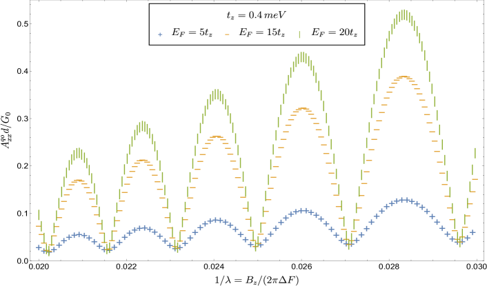
(a) The amplitude of quantum oscillations of normalized in-plane diagonal conductivity $A_{xx}^{qo}d/G_{0}$ given by Eq. (41) as a function of $1/\lambda\sim B_{z}$ (here $G_{0}=e^{2}/(\pi\hbar)$ is the quantum of conductance) for three different values of Fermi energy $E_{F}$. The positions of local minima of MQO amplitude (beat nodes) do not depend on Fermi energy $E_{F}$, but the amplitude of MQO amplitude does according to Eq. (41) and discussion after Eq. (42). The taken parameters are: $m_{\ast}=0.04m_{e}$, $\Gamma_{0}=14.5\,K$, $t_{z}=10\,meV$, $E_{F}=\{5,\,10,\,20\}t_{z}$.

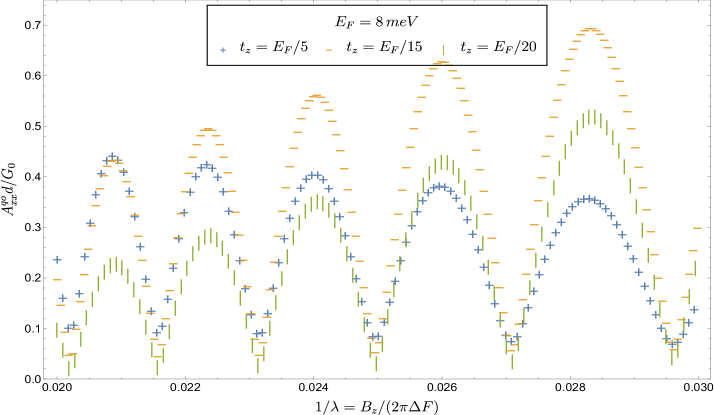
(b) The same as in Fig. (a) at fixed $E_{F}$ but for three different values of $t_{z}$. The values at local minima of MQO depend on $t_{z}$. The taken parameters are: $m_{\ast}=0.04m_{e}$, $\Gamma_{0}=14.5\,K$, $t_{z}=\{1/5,\,1/15,\,1/20\}E_{F}$, $E_{F}=200\,meV$.

Figure 1: The amplitude of quantum oscillations of in-plane diagonal conductivity for three different ratios $t_{z}/E_{F}$.

To find the fast quantum oscillations of $\sigma_{xx}^{(1)}(\varepsilon)$ in the lowest order in $R_{D}J_{0}(\lambda)$ it is sufficient to replace $\gamma$ by $\gamma_{0}$ and $\alpha(\varepsilon_{\ast})$ by its average value $\overline{\alpha}$ in Eq. (23):

$$\sigma_{xx}^{(1)}(\varepsilon)_{qo}\approx-2\overline{\sigma}_{xx}^{(0)}R_{D}\left[J_{0}(\lambda)\cos\left(\overline{\alpha}\right)-\frac{\lambda}{\overline{\alpha}}J_{1}(\lambda)\sin(\overline{\alpha})\right].$$ (38)

Then, the sum of Eqs. (36) and (38) gives the total fast quantum oscillations in the first order in $R_{D}J_{0}(\lambda)$:

$$\sigma_{xx}^{qo}(\varepsilon)=\sigma_{xx}^{(0)}(\varepsilon)_{qo}+\sigma_{xx}^{(1)}(\varepsilon)_{qo}\approx$$

$$\approx-2\overline{\sigma}_{xx}^{(0)}R_{D}\left[\frac{2\pi^{2}J_{0}\left(\lambda\right)}{\gamma_{0}^{2}+\pi^{2}}\cos\left(\overline{\alpha}\right)-\frac{\lambda}{\overline{\alpha}}J_{1}(\lambda)\sin(\overline{\alpha})\right].$$ (39)

We transform this trigonometric expression to

$$\sigma_{xx}^{qo}(\varepsilon)\approx-A_{xx}^{qo}\cos(\overline{\alpha}+\Delta\phi_{qo}),$$ (40)

where the amplitude of MQO is given by

$$A_{xx}^{qo}=2\overline{\sigma}_{xx}^{(0)}R_{D}\sqrt{\frac{4\pi^{4}}{(\gamma_{0}^{2}+\pi^{2})^{2}}J_{0}^{2}(\lambda)+\left(\frac{\lambda}{\overline{\alpha}}\right)^{2}J_{1}^{2}(\lambda)}$$ (41)

and a phase shift of MQO is

$$\Delta\phi_{qo}=$$

$$=\arccos\left[\frac{2\pi^{2}J_{0}\left(\lambda\right)\overline{\alpha}}{\sqrt{(2\pi^{2}J_{0}\left(\lambda\right)\overline{\alpha})^{2}+\left(\lambda J_{1}(\lambda)\left(\gamma_{0}^{2}+\pi^{2}\right)\right)^{2}}}\right].$$ (42)

This phase shift jumps by $\sim\pi$ and changes the sign of $\sigma_{xx}^{qo}$ at certain values of magnetic field, corresponding to the beats of MQO at $J_{0}\left(\lambda\right)=0$. The second term in the denominator makes this phase jump smoother and is missing in phenomenological theoriesGrigEuroPhys2016 ; MQOYBCOPRB .

The derived expressions (39–42), describing the MQO of in-plane conductivity in the lowest non-vanishing order in $R_{D}J_{0}(\lambda)$, have several important features. Due to the second term in Eq. (39), the MQO amplitude $A_{xx}^{qo}$, given by Eq. (41) and plotted in Fig. 1, is nonzero even at beat nodes $J_{0}(\lambda)=0$, corresponding to the minima of MQO amplitude, where it increases with the increase of ratio $\lambda/\overline{\alpha}=2t_{z}/E_{F}$. At maxima the MQO amplitude $A_{xx}^{qo}$ is proportional to the square of electron velocity and, for a parabolic in-plane electron dispersion, to the Fermi energy $E_{F}$, in agreement with the standard theoryShoenberg (see Fig. 1a). Eqs. (39) and (41) suggest that at $\gamma_{0}\gtrsim\pi$, in addition to the standard Dingle factor, the MQO are damped by the factor $1/(\gamma_{0}^{2}+\pi^{2})$. We illustrate all this in Fig. 1 by plotting the amplitude $A_{xx}^{qo}$ as a function of $1/\lambda=B_{z}/(2\pi\Delta F)$ for three different ratios of $t_{z}/E_{F}$. In Fig. 1a we keep $t_{z}$ fixed and vary $E_{F}$, which may correspond to different Fermi-surface pockets or Fermi-surface reconstruction, and in Fig. 1b we keep $E_{F}$ fixed and vary $t_{z}$. In all figures the MQO amplitude increases with the increase of magnetic field because of the Dingle factor. In Fig. 1a at the beat nodes the MQO amplitude is the same for all three curves because $E_{F}^{-1}$ in the factor $t_{z}/E_{F}$ is compensated by the overall factor $E_{F}$ in $\overline{\sigma}_{xx}^{(0)}$. In Fig. 1b three different curves, corresponding to various values of $t_{z}$, also correspond to different magnetic field strength, because we plotted $A_{xx}^{qo}$ as function of $1/\lambda\propto B_{z}/t_{z}$. Therefore, at low field the blue curve, corresponding to $t_{z}=E_{F}/5$, is higher at MQO maxima. The second term in Eq. (39) also results to additional phase shift in Eq. (42), which depends on magnetic field via $\lambda$ and $\gamma_{0}$ and is essential only near the beat nodes $J_{0}\left(\lambda\right)=0$, as illustrated in Fig. 2.

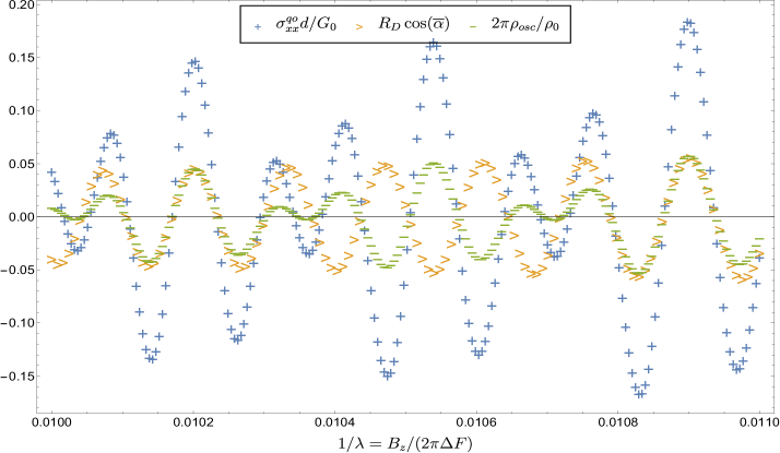
Figure 2: Quantum oscillations of in-plane diagonal conductivity as compared to $R_{D}\cos(\overline{\alpha})$ and to the oscillating part $\rho_{osc}$ of the DoS, where $\rho_{osc}\equiv-2\rho_{0}\cos(\overline{\alpha})R_{D}J_{0}(\lambda)$. The phases of DoS and of $\sigma_{xx}$ oscillations coincide everywhere except the proximity of beat nodes. The taken parameters are: $m_{\ast}=0.04m_{e}$, $\Gamma_{0}=14.5\,K$, $t_{z}=20\,meV$, $E_{F}=200\,meV$.

To find the slow oscillations of $\sigma_{xx}^{(1)}(\varepsilon)$ in the lowest (second) order in $R_{D}J_{0}(\lambda)$ we need to expand $\gamma$ in (23) according to Eq. (33) and take into account oscillations of $\alpha$. This expansion gives

$$\sigma_{xx}^{(1)}(\varepsilon)-\sigma_{xx}^{(1)}(\varepsilon)_{qo}\approx 4\overline{\sigma}_{xx}^{(0)}\frac{\pi^{2}-\gamma_{0}^{2}}{\gamma_{0}^{2}+\pi^{2}}R_{D}^{2}J_{0}\left(\lambda\right)\times$$

$$\times\cos\left(\overline{\alpha}\right)\left[J_{0}(\lambda)\cos\left(\overline{\alpha}\right)-\frac{\lambda}{\overline{\alpha}}J_{1}(\lambda)\sin(\overline{\alpha})\right],$$ (43)

and the SlO coming from this expression are given by

$$\sigma_{xx}^{(1)}(\varepsilon)_{so}\approx 2\overline{\sigma}_{xx}^{(0)}(\varepsilon)\frac{\pi^{2}-\gamma_{0}^{2}}{\gamma_{0}^{2}+\pi^{2}}R_{D}^{2}J_{0}^{2}\left(\lambda\right).$$ (44)

The total SlO of diagonal in-plane conductivity are given by the sum of Eqs. (37) and (44):

$$\sigma_{xx}^{so}(\varepsilon)\approx 2\pi^{2}\overline{\sigma}_{xx}^{(0)}R_{D}^{2}J_{0}^{2}\left(\lambda\right)\frac{\pi^{2}-3\gamma_{0}^{2}}{(\gamma_{0}^{2}+\pi^{2})^{2}}.$$ (45)

To summarize the calculations, the harmonic expansion (by the parameter $\gamma_{1}\equiv 2\gamma_{0}R_{D}J_{0}\left(\lambda\right)\ll 1$) of intralayer conductivity $\sigma_{xx}(\varepsilon)$ is given by the sum of three main terms:

$$\sigma_{xx}(\varepsilon)\approx\overline{\sigma}_{xx}^{(0)}(\varepsilon)+\sigma_{xx}^{qo}(\varepsilon)+\sigma_{xx}^{so}(\varepsilon),$$ (46)

where the term $\overline{\sigma}_{xx}^{(0)}(\varepsilon)$ corresponds to the nonoscillating part of conductivity and is given by Eq. (35), $\sigma_{xx}^{qo}(\varepsilon)$ describes the MQO of intralayer conductivity, given by Eq. (39), and $\sigma_{xx}^{so}(\varepsilon)$ describes the slow oscillations of intralayer conductivity and is given by Eq. (45).

III.3 Damping by temperature and sample inhomogeneities

As was shown in Refs. [SO, ; Shub, ; MQOYBCOPRB, ], the smearing of the Fermi level by temperature and by long-range sample inhomogeneities damps only the fast MQO $\sigma_{xx}^{qo}(\varepsilon)$, and does not affect the constant part $\overline{\sigma}_{xx}^{(0)}(\varepsilon)$ or the SlO $\sigma_{xx}^{so}(\varepsilon)$. Indeed, at finite temperature $T$ conductivity $\sigma_{xx}=\sigma_{xx}\left(T\right)$ is given by the integral of $\sigma_{xx}(\varepsilon)$ over electron energy $\varepsilon$ weighted by the derivative of Fermi distribution function $n_{F}^{\prime}(\varepsilon)=-1/\{4T\cosh^{2}\left[(\varepsilon-\mu)/(2T)\right]\}$ with the chemical potential $\mu=E_{F}$:

$$\sigma_{xx}\left(\mu,\,T\right)=\int d\varepsilon\,\left[-n_{F}^{\prime}(\varepsilon)\right]\,\sigma(\varepsilon).$$ (47)

Among the three terms in Eq. (46) only the second term $\sigma_{xx}^{qo}(\varepsilon)$, describing MQO, is a rapidly oscillating function of electron energy $\varepsilon$ because of its dependence on $\overline{\alpha}\left(\varepsilon\right)$. As a result of the integration over $\varepsilon$, only this term acquires the additional temperature damping factor

$$R_{T}=(2\pi^{2}k_{B}T/(\hbar\omega_{c}))/\sinh\left(2\pi^{2}k_{B}T/(\hbar\omega_{c})\right),$$ (48)

and the electron energy $\varepsilon$ is replaced by the chemical potential $\mu$. The macroscopic spatial inhomogeneities smear the Fermi energy along the whole sample. Hence, in addition to the temperature smearing in Eq. (47), given by the integration over electron energy $\varepsilon$, conductivity $\sigma$ acquires the coordinate smearing, given by the integration over Fermi energy $\mu$ around its average value $\mu_{0}$ weighted by a normalized distribution function $D\left(\mu\right)=D_{0}\left[\left(\mu-\mu_{0}\right)/W\right]$ of width $W$ : $\sigma=\int d\mu\,\sigma(\mu)D\left(\mu\right)$. Again, only the second term $\sigma_{xx}^{qo}$, describing MQO, is a rapidly oscillating function of $\mu$ via $\overline{\alpha}\left(\mu\right)$, and only this term acquires additional damping factor

$$R_{W}=\int dxD_{0}\left(x\right)\cos\left(2\pi xW/(\hbar\omega_{c})\right)=R_{W}(W/(\hbar\omega_{c})),$$ (49)

due to the sample inhomogeneities. This damping of MQO by long-range sample inhomogeneities in layered organic metal $\beta$-(BEDT-TTF)₂IBr₂ was shown to be much stronger than the damping by usual short-range impuritiesSO , making the amplitude of SlO much larger than of MQO. The SlO, given by Eq. (45), do not depend on $\mu$ and, hence, are not damped by the factor $R_{W}$. This property makes the observation of SlO much easier than of MQO. It was used in the alternative interpretationMQOYBCOJETPL ; MQOYBCOPRB of the observedHusseyNature2003 ; ProustNature2007 ; SebastianNature2008 ; AudouardPRL2009 ; SingletonPRL2010 ; SebastianPNAS2010 ; SebastianPRB2010 ; SebastianPRL2012 ; SebastianNature2014 ; ProustNatureComm2015 MQO in YBCO high-temperature superconductors.

III.4 Influence of electron spin on conductivity

All previous expressions are for spinless electrons. If we take into account the spin splitting of Fermi level $E_{F}\pm\frac{1}{2}g\mu_{e}|\bm{B}|$ ($g$ is the electron $g$-factor, $\mu_{e}$ is the Bohr magneton) and sum expressions (35) for Drude conductivity over both spin components, we simply multiply the spinless result (35) by two:

$$\overline{\sigma}_{xx}^{(0)}(\varepsilon)\approx\frac{e^{2}}{2\pi\hbar d}\frac{\overline{\alpha}\gamma_{0}}{\gamma_{0}^{2}+\pi^{2}}.$$ (50)

For MQO $\sigma_{xx}^{qo}$, given by Eq. (39), the sum of both spin components gives

$$\sigma_{xx}^{qo}(\varepsilon)\approx-2\overline{\sigma}_{xx}^{(0)}R_{D}R_{S}\times$$

$$\times\left[\frac{2\pi^{2}J_{0}\left(\lambda\right)}{\gamma_{0}^{2}+\pi^{2}}\cos\left(\overline{\alpha}\right)-\frac{\lambda}{\overline{\alpha}}J_{1}(\lambda)\sin(\overline{\alpha})\right],$$ (51)

where the spin damping factor $R_{S}$ of MQO in quasi-2D metals with $t_{z}\ll E_{F}$ is $R_{S}=\cos\left[\pi gm_{\ast}/(2m_{e}\cos\theta)\right]$ ($m_{e}$ is the free electron mass).

The influence of spin splitting on SlO depends on electron dispersion and on the coupling between two spin components. For the parabolic in-plane dispersion, given by Eq. (3), and in the absence of any coupling between two spin components, the Zeeman spin splitting only adds a factor of $2$ to $\sigma_{xx}^{so}$, similar to the Drude term. Indeed, the SlO term in Eq. (45) does not depend on energy, and the sum over two spin-split energy bands only adds a factor of $2$ to final expression. However, for a more complicated in-plane electron dispersion this simple conclusion may violate. Moreover, in real compounds there is often some coupling between two spin components due to spin-dependent scattering, chemical-potential oscillations and oscillating magnetostriction, or other effects. This coupling between two spin components introduces additional terms to SlO, which may lead to the angular dependence of SlO amplitude and even to an analogue of the spin-zero effect.

III.5 The limiting cases of large and small interlayer transfer integrals $t_{z}$

In this section we compare the results obtained with two previously know limiting cases, namely, 2D and 3D. The SlO are specific to quasi-2D metals, being neglected in both these limiting case. In 2D case, $t_{z}=0$, the SlO have zero frequency and, hence, do not exist. In 3D metals, where $t_{z}\sim E_{F}\gg\hbar\omega_{c}$, the SlO may exist but have too small amplitude, being less than MQO by a factor $\sim R_{D}\sqrt{\hbar\omega_{c}/(2\pi^{2}t_{z})}\ll 1$. Hence, below we compare only the usual MQO of intralayer conductivity.

In the 2D limiting case, taking $t_{z}=0$ and $\lambda=0$ in Eq. (39), we obtain the following expression for the MQO of intralayer conductivity

$$\sigma_{xx}^{qo}(\varepsilon,\,t_{z}=0)\approx-\overline{\sigma}_{xx}^{(0)}R_{D}\frac{4\pi^{2}}{\gamma_{0}^{2}+\pi^{2}}\cos\left(\overline{\alpha}\right).$$ (52)

It coincides with Eq. (2.15) of Ref. [AndoIV, ], where the quantum transport in a 2D electron system under magnetic fields was studied. Note that the amplitude of MQO in this Eq. (2.15) of Ref. [AndoIV, ] is twice larger than in Eq. (2.16) of the same workAndoIV or in Eq. (6.40) of Ref. [AndoFowlerSternRMP82, ], where the quantum oscillations of $\text{Im}\Sigma$ or $\tau$ are neglected.

The limiting 3D case corresponds to large $t_{z}\gg\hbar\omega_{c}$, i.e., $\lambda\gg 1$. In this limit one may use asymptotic expansions of the Bessel functions at large argument in Eq. (39): $J_{0}(\lambda)\approx\sqrt{2/(\pi\lambda)}\cos(\lambda-\pi/4)$, $J_{1}(\lambda)\approx\sqrt{2/(\pi\lambda)}\sin(\lambda-\pi/4)$. Then Eq. (39) simplifies to

$$\sigma_{xx}^{qo}(\varepsilon)\approx-\left(\frac{2^{3}}{\pi\lambda}\right)^{1/2}\overline{\sigma}_{xx}^{(0)}R_{D}\left[\frac{2\pi^{2}\cos\left(\overline{\alpha}\right)}{\gamma_{0}^{2}+\pi^{2}}\cos\left(\lambda-\frac{\pi}{4}\right)\right.-$$

$$\left.-\frac{\lambda}{\overline{\alpha}}\sin(\overline{\alpha})\sin\left(\lambda-\frac{\pi}{4}\right)\right].$$ (53)

In a strong magnetic field $\gamma_{0}\ll 1$, $R_{D}\approx 1$, and Eq. (53) in terms of initial parameters reduces to

$$\frac{\sigma_{xx}^{qo}(\varepsilon)}{\overline{\sigma}_{xx}^{(0)}}\approx-\frac{2}{\pi}\left(\frac{2\hbar\omega_{c}}{t_{z}}\right)^{1/2}\times$$

$$\times\left[\cos\left(\frac{2\pi E_{F}}{\hbar\omega_{c}}\right)\cos\left(\frac{4\pi t_{z}}{\hbar\omega_{c}}-\frac{\pi}{4}\right)\right.-$$

$$\left.-\frac{2t_{z}}{E_{F}}\sin\left(\frac{2\pi E_{F}}{\hbar\omega_{c}}\right)\sin\left(\frac{4\pi t_{z}}{\hbar\omega_{c}}-\frac{\pi}{4}\right)\right].$$ (54)

We compare Eq. (54) with the expression obtained in Ref. [LifhitzKosevich, ] (see Eq. (4) of Ref. [LifhitzKosevich, ]) and written in a more convenient form in Eq. (90.22) of the textbookLandauLifhitzKinetiks :

$$(\sigma_{xx})_{A}=\sum_{ex}\sum_{l=1}^{+\infty}(-1)^{l}\sigma_{xx}^{(l)}\cos\left\{l\frac{cS_{ex}}{e\hbar B_{z}}\pm\frac{\pi}{4}\right\},$$ (55)

where $ex\equiv\{min,\,max\}$ means extremal cross-section of the Fermi surface,

$$\sigma_{xx}^{(l)}=\frac{2^{5/2}\pi^{1/2}(e\hbar)^{1/2}b_{ex}}{c^{1/2}B_{z}^{3/2}l^{1/2}}\left|\frac{\partial^{2}S}{\hbar^{2}\partial k_{z}^{2}}\right|_{ex}^{-1/2},$$ (56)

$b_{ex}$ is the quantity $b_{z}(E_{F},\,k_{z\,ex}(E_{F}))$ given by Eqs. (90.13) and (90.15) of the book LandauLifhitzKinetiks and taken at points $k_{z\,ex}$, corresponding to Fermi surface extremal cross sections. The “$\pm$” in Eq. (55) means “$-$” for maximum and “$+$” for minimum of the function $S_{ex}(k_{z})$.

In our case there are two extremal cross sections over the period $2\pi/d$. These extremal cross section areas of the Fermi surface are

$$S_{ex}=2\pi m_{\ast}(E_{F}+2t_{z}\cos(k_{z}d))|_{ex}=2\pi m_{\ast}(E_{F}\pm 2t_{z}).$$ (57)

Their second derivatives at extremal points are

$$\frac{\partial^{2}S}{\hbar^{2}\partial k_{z}^{2}}|_{ex}=-\frac{4\pi m_{\ast}d^{2}t_{z}}{\hbar^{2}}\cos(k_{z}d)|_{ex}=\mp\frac{4\pi m_{\ast}d^{2}t_{z}}{\hbar^{2}}.$$ (58)

If we assume that $b_{max}=b_{min}$, which is valid at least if $t_{z}\ll E_{F}$, the sum over extremal cross sections for $l=1$ in Eq. (55) can be simplified:

$$\sum_{ex}\cos\left\{\frac{cS_{ex}}{e\hbar B_{z}}\pm\frac{\pi}{4}\right\}=2\cos\left(\frac{2\pi E_{F}}{\hbar\omega_{c}}\right)\cos\left(\frac{4\pi t_{z}}{\hbar\omega_{c}}-\frac{\pi}{4}\right).$$ (59)

Using auxiliary Eqs. (56), (58), and (59) in Eq. (55), we find the oscillating part of intralayer conductivity for the first harmonic $l=1$

$$(\sigma_{xx}^{qo})_{A}\approx-\sqrt{\frac{2^{5}e\hbar^{3}b_{max}^{2}}{m_{\ast}cB^{3}_{z}t_{z}d^{2}}}\cos\left(\frac{2\pi E_{F}}{\hbar\omega_{c}}\right)\cos\left(\frac{4\pi t_{z}}{\hbar\omega_{c}}-\frac{\pi}{4}\right).$$ (60)

From the Eq. (90.15) on p. 387 of the bookLandauLifhitzKinetiks one can evaluate the intralayer conductivity $\sigma_{xx}$ averaged over the period of magnetic oscillations

$$(\overline{\sigma}_{xx})_{A}=\frac{2\hbar}{B_{z}^{2}}\int_{-\pi/d}^{\pi/d}b(E_{F},\,k_{z})dk_{z}\approx\frac{4\pi\hbar b_{max}}{dB_{z}^{2}}.$$ (61)

Finally, gathering Eqs. (60) and (61), we find the ratio of oscillating and non-oscillating parts:

$$\frac{(\sigma_{xx}^{qo})_{A}}{(\overline{\sigma}_{xx})_{A}}\approx-\left(\frac{2\hbar\omega_{c}}{\pi^{2}t_{z}}\right)^{1/2}\cos\left(\frac{2\pi E_{F}}{\hbar\omega_{c}}\right)\cos\left(\frac{4\pi t_{z}}{\hbar\omega_{c}}-\frac{\pi}{4}\right).$$ (62)

This is twice smaller than in Eq. (54), because in the derivation of Eqs. (55–62) the quantum oscillations of $b_{ex}$, and, hence, of $\text{Im}\Sigma$ are neglected. This extra factor of two, arising from the oscillations of $\text{Im}\Sigma$, is similar to that in the 2D case discussed above. If we neglected the MQO of $\text{Im}\Sigma$, instead of Eq. (39) we would use Eq. (38). Then, performing similar expansion as in the derivation of Eqs. (53) and (54), from Eq. (38) we obtain Eq. (62) in the lowest order in $t_{z}/E_{F}$.

IV Discussion

The calculations of intralayer conductivity in the previous section shows that $\sigma_{xx}(\mu)$ can be divided into three parts:

$$\sigma_{xx}(\mu,\,T)\approx\overline{\sigma}_{xx}^{(0)}(\mu)+\sigma_{xx}^{qo}(\mu)R_{T}R_{W}+\sigma_{xx}^{so}(\mu),$$ (63)

where $\overline{\sigma}_{xx}^{(0)}(\mu)$ represents the nonoscillating part of conductivity, given by Eq. (35), $\sigma_{xx}^{qo}(\mu)$ describes the MQO of intralayer conductivity, given by Eq. (39), and $\sigma_{xx}^{so}(\mu)$ describes the slow oscillations of intralayer conductivity, given by Eq. (45). The second term, representing MQO, acquires two damping factors $R_{T}$ and $R_{W}$ from temperature and macroscopic sample inhomogeneities.

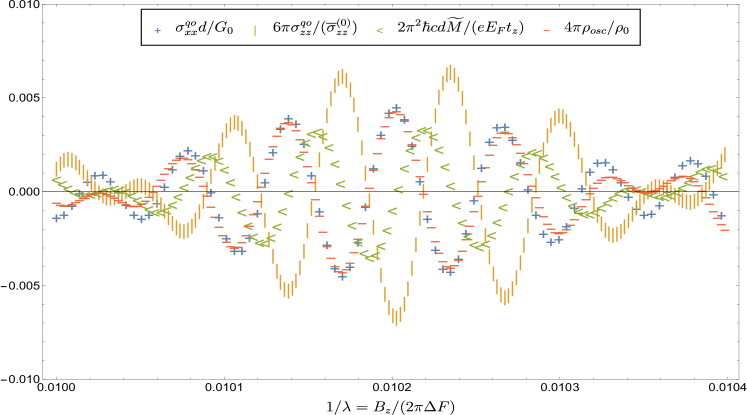
Figure 3: Quantum oscillations of intralayer diagonal conductivity $\sigma_{xx}^{qo}$, of interlayer conductivity $\sigma_{zz}^{qo}$, and of magnetization $\widetilde{M}$ as a function $1/\lambda=B_{z}/(2\pi\Delta F)$. One can see that the oscillations of $\sigma_{zz}^{qo}$ are shifted from $\widetilde{M}$ by a quarter of period, but at $1/\lambda\approx 0.01036$ the phase shift is close to $\pi$. Except the beat nodes, the oscillations of $\sigma_{xx}$ have the same phase as those of the density of states, but are in antiphase with the oscillations of $\sigma_{zz}$. The parameters for numerical calculations are: $m_{\ast}=0.04m_{e}$, $\Gamma_{0}=14.5\,K$, $t_{z}=10\,meV$, $E_{F}=200\,meV$.

The quantum oscillations of interlayer conductivity $\sigma_{zz}^{qo}(\mu)$, instead of Eq. (39), are given by Eq. (18) of Ref. [Shub, ], which can be rewritten as

$$\sigma_{zz}^{qo}(\mu)\approx 2\overline{\sigma}_{zz}^{(0)}\cos\left(\overline{\alpha}\right)R_{D}\left[J_{0}\left(\lambda\right)-\frac{2}{\lambda}\left(1+\gamma_{0}\right)J_{1}\left(\lambda\right)\right].$$ (64)

Let us compare Eq. (39) for $\sigma_{xx}^{qo}$ with Eq. (64) for $\sigma_{zz}^{qo}$. They look similar but have several important differences: (i) the total sign “$-$”, responsible for the phase shift $\pi$ of MQO of in-plane $\sigma_{xx}$ with respect to interlayer $\sigma_{zz}$ conductivity, (ii) the amplitude of MQO of $\sigma_{xx}$, given by Eq. (41), is nonzero even in the beat nodes; (iii) additional field-dependent phase shift of MQO of intralayer conductivity, given by Eq. (42), and (iv) the expression in the square brackets in Eq. (64), responsible for the amplitude oscillations (beats) of MQO of interlayer conductivity, contains extra term $\propto J_{1}\left(\lambda\right)$, which gives the field-dependent phase shift $\phi_{b}$ of beats of MQO of $\sigma_{zz}$PhSh ; Shub . This phase shift $\phi_{b}$ contains the parameter $2\left(1+\gamma_{0}\right)/\lambda=\left(1+\gamma_{0}\right)\hbar\omega_{c}/(2\pi t_{z}$), which is not small in strongly anisotropic Q2D metals. This factor increases with the increase of magnetic field; it is $\sim 1$ in strongly anisotropic Q2D metals and $\ll 1$ in weakly anisotropic almost 3D metals. For the in-plane conductivity $\sigma_{xx}$ in Eq. (39) similar term results not in the phase shift of beats, but in the phase shift of MQO themselves, given by Eq. (42). It is small by the parameter $\lambda/\overline{\alpha}=2t_{z}/E_{F}$ and is approximately field-independent. In strongly anisotropic Q2D metals $2t_{z}/E_{F}\ll 1$, and this phase shift is negligibly small. However, in weakly anisotropic Q2D metals this parameter $\lambda/\overline{\alpha}=2t_{z}/E_{F}\sim 1$, although they have a cylindrical Fermi surface and are far from the Lifshitz transition and magnetic breakdown, i.e., $E_{F}-2t_{z}\gg\hbar\omega_{c}$.

To measure the proposed phase shift of fast Shubnikov oscillations one can compare the phase of Shubnikov and de Haas - van Alphen oscillations. The latter are determined by the oscillations of DoSChampelMineevPhilMag ; Grig2001

$$\rho(B_{z})\approx\rho_{0}\left[1-2R_{D}J_{0}(\lambda)\cos\left(\overline{\alpha}\right)\right]\text{,}$$ (65)

where the nonoscillating part of the DOS (per one spin) is $\rho_{0}=m_{\ast}/(2\pi\hbar^{2}d)$, and the magnetization oscillations per one spin component are given byGrig2001 ; Champel2001 ; Shub

$$\widetilde{{M}}(B_{z})\approx\frac{eE_{F}}{2\pi^{2}\hbar cd}R_{D}R_{T}\times$$

$$\times\left(J_{0}(\lambda)\sin\left(\overline{\alpha}\right)+\frac{\lambda}{\overline{\alpha}}J_{1}(\lambda)\cos\left(\overline{\alpha}\right)\right)\text{.}$$ (66)

Eqs. (65) and (66) are illustrated in Fig. 3 and compared to conductivity oscillations.

At low magnetic field, when $\lambda\gg 1$, the second term in the square brackets of Eq. (64) is small, and the MQO of $\sigma_{zz}$ in Eq. (64) and of $\sigma_{xx}$ in Eq. (39) are in antiphase. Note that the phase of $\sigma_{xx}$ MQO coincides with the phase of DoS MQO given by Eq. (65). This is illustrated in Fig. 3. However, at high fields ${\hbar\omega_{c}\gg 4\pi t_{z}}$ expression (64) for interlayer conductivity $\sigma_{zz}^{qo}$ asymptotically is equal to $-2\overline{\sigma}_{zz}^{(0)}\cos\left(\overline{\alpha}\right)R_{D}\left[1+2\gamma_{0}\right]$, while $\sigma_{xx}^{qo}$ is close to $-4\pi^{2}\overline{\sigma}_{xx}^{(0)}R_{D}\cos\left(\overline{\alpha}\right)/\left(\gamma_{0}^{2}+\pi^{2}\right)$. Hence, at high magnetic fields the fast oscillations of $\sigma_{xx}$, $\sigma_{zz}$ and DoS have the same phase. This agrees with the calculations of $\sigma_{zz}$ within the two-layer modelWIPRB2011 ; WIPRB2012 ; Grigbro ; TarasPRB2014 ; TarasPRB2017 and for 3D dispersion (4) at $\hbar\omega_{c}\gg t_{z}$ChampelMineev ; GrigPRB2013 . Hence, there is a crossover between these two regimes of $\sigma_{zz}$ at $\lambda\sim 1$.

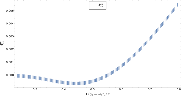
(a) Amplitude $A^{so}_{xx}$ of slow oscillations of normalized intralayer diagonal conductivity $\sigma_{xx}^{so}d/G_{0}$ as a function of $1/\gamma_{0}=\hbar\omega_{c}/(2\pi\Gamma_{0})\propto B_{z}$. This plot demonstrates that the amplitude $A^{so}_{xx}$ changes its sign at $\gamma_{0}=\pi/\sqrt{3}$.

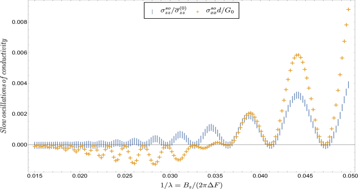
(b) Slow oscillations of intralayer $\sigma_{xx}$ and interlayer $\sigma_{zz}$ conductivity as a function of $1/\lambda=\hbar\omega_{c}/(4\pi t_{z})\propto B_{z}$. The slow oscillations of $\sigma_{xx}$ and $\sigma_{zz}$ are in antiphase at low magnetic field and have the same phase at high field.

Figure 4: The amplitude (a) and magnitude (b) of slow oscillations of $\sigma_{xx}$ and $\sigma_{zz}$. The parameters are the same as in Fig. 3.

Let us now compare Eq. (45) for $\sigma_{xx}^{so}(\varepsilon)$ with the slow oscillations of interlayer conductivity $\sigma_{zz}^{so}(\varepsilon)$, given by Eqs. (18) or (19) of Ref. [Shub, ], which can be rewritten as

$$\sigma_{zz}^{so}(\mu)\approx 2\overline{\sigma}_{zz}^{(0)}R_{D}^{2}J_{0}\left(\lambda\right)\left[J_{0}\left(\lambda\right)-\frac{2}{\lambda}J_{1}\left(\lambda\right)\right].$$ (67)

Similar to the beats of fast MQO, the slow oscillations of interlayer conductivity $\sigma_{zz}$ have a field-dependent phase shift due to the second term $2J_{1}\left(\lambda\right)/\lambda$ in the square brackets of Eq. (67), which is absent in the SlO of $\sigma_{xx}$. This phase shift $\phi_{s}^{zz}\sim 2/\lambda$ is small at $\lambda\gg 1$, i.e., everywhere except the last period of slow oscillations.

The main difference of the SlO of interlayer $\sigma_{zz}^{so}$ and intralayer $\sigma_{xx}^{so}$ conductivity is that the amplitude of the latter depends nonmonotonically on $\gamma_{0}=\pi/(\omega_{c}\tau_{0})$, as one can see from Eq. (45): at $\gamma_{0}^{2}=\pi^{2}/3$ the amplitude of SlO of $\sigma_{xx}$ changes sign, going through zero. At small $\gamma_{0}<\pi/\sqrt{3}$, i.e., at large $\omega_{c}\tau_{0}>\sqrt{3}$ when MQO are strong, the slow oscillations of intralayer $\sigma_{xx}$ and interlayer $\sigma_{zz}$ conductivity are in the same phase. At large $\gamma_{0}>\pi/\sqrt{3}$, i.e., at small $\omega_{c}\tau_{0}<\sqrt{3}$ when MQO are weak, the SlO of $\sigma_{xx}$ and $\sigma_{zz}$ are in the antiphase. To demonstrate this phase shift $\pi$ of SlO of in-plane conductivity $\sigma_{xx}$ with respect to interlayer conductivity $\sigma_{zz}$, in Fig. 4a we plot the amplitude

$$A_{xx}^{so}\equiv\frac{\pi}{2\lambda}\overline{\alpha}\gamma_{0}R_{D}^{2}\frac{\pi^{2}-3\gamma_{0}^{2}}{(\gamma_{0}^{2}+\pi^{2})^{3}}$$ (68)

of $\sigma_{xx}^{so}d/G_{0}$, where $G_{0}=e^{2}/(\pi\hbar)$ is the quantum of conductance (the expression for the amplitude follows from the expression of $\sigma_{xx}^{so}d/G_{0}$ after using the asymptote of squared Bessel function $J^{2}_{0}(\lambda)\sim(1+\sin(2\lambda))/(\pi\lambda)$ for $\lambda\gg 1$ and extracting the coefficient before $\sin(2\lambda)$). In Fig. 4b we compare $\sigma_{xx}^{so}d/G_{0}$ given by Eq. (45) to $\sigma_{zz}^{so}d/G_{0}$ given by Eq. (67). Contrary to $\sigma_{xx}^{so}$, the amplitude of SlO of interlayer conductivity $\sigma_{zz}^{so}$ in Eq. (67) monotonically decreases with increasing $\gamma_{0}$ (see Fig. 4). The nonmonotonic field dependence of the amplitude of slow oscillations of in-plane conductivity, probably, explains the $\pi$-difference of the phase of SlO of in-plane magnetoresistance observedGrigEuroPhys2016 in rare-earth tritellurides TbTe₃ and GdTe₃ (see Fig. 6 of Ref. [GrigEuroPhys2016, ]).

V Summary

To summarize, we calculate the magnetic quantum oscillations (MQO) of intralayer conductivity $\sigma_{xx}$ in quasi-2D metals in quantizing magnetic field. This calculation is based on the Kubo formula and harmonic expansion. It takes into account the electron scattering by short-range impurities and neglects the electron-electron interaction. The latter approximation is justified in the metallic limit of large number of filled LLs and finite interlayer transfer integral $t_{z}$. Previously, such calculation in quasi-2D metals was performed only for interlayer conductivity $\sigma_{zz}$ChampelMineev ; Shub . We calculated analytically the amplitudes and phases of the usual MQO and the so-called slow oscillations (SlO) with frequency $\propto t_{z}$, arising from the mixing of two close MQO frequencies. The SlO appear only in the second order in the Dingle factor, but they are usually stronger than MQO, because the latter are additionally damped by temperature and sample inhomogeneities.

The comparison of the results for intralayer $\sigma_{xx}$ and interlayer $\sigma_{zz}$ conductivity shows several qualitative differences between their oscillations, discussed and illustrated above. The amplitude of SlO of $\sigma_{xx}$, given by Eqs. (45) and (68) and illustrated in Fig. 4, has a nonmonotonic dependence on magnetic field. This amplitude changes sign at $\gamma_{0}=\pi/(\omega_{c}\tau_{0})=\pi/\sqrt{3}$, while the amplitude of SlO of $\sigma_{zz}$ is a monotonic function of field. The SlO of $\sigma_{xx}$ and $\sigma_{zz}$ have opposite phase in weak magnetic field and same phase in strong field. The MQO of $\sigma_{zz}$ have a crossover with a phase inversion at $\lambda\sim 1$, while MQO of $\sigma_{xx}$ do not have such crossover. Therefore, similarly to SlO, the MQO of $\sigma_{zz}$ and $\sigma_{xx}$ have opposite phase in weak magnetic field and same phase in strong field. This crossover between high- and low-field limits for MQO of $\sigma_{zz}$ is driven by the parameter $\lambda=4\pi t_{z}/(\hbar\omega_{c})$, while for SlO of $\sigma_{xx}$ the driving parameter is $\gamma=2\pi\Gamma/(\hbar\omega_{c})$.

Notably, the oscillations of MQO amplitudes, called beats and arising from the interference of two close frequencies, for $\sigma_{xx}$ are not complete, i.e., the amplitude of $\sigma_{xx}$ oscillations is nonzero even in the beat nodes, as given by Eq. (41) and illustrated in Fig. 1. The field-dependent phase shift of beats, known for $\sigma_{zz}$ MQOPhSh ; Shub , does not appear in $\sigma_{xx}$. However, for $\sigma_{xx}$ the phase of MQO themselves is shifted by the value $\,\sim t_{z}/E_{F}$, as given by Eqs. (39), (42).

The developed theory and the results obtained are applicable to describe transverse magnetoresistance in various anisotropic quasi-2D conductors, including organic metals, high-Tc superconducting materials, heterostructures, intercalated graphite, rare-earth tritellurides, etc.

- (1) A. A. Abrikosov, Fundamentals of the theory of metals, (North-Holland, Amsterdam, 1988).
- (2) J. M. Ziman, Principles of the Theory of Solids (Cambridge University Press, Cambridge, 1972).
- (3) D. Shoenberg, Magnetic oscillations in metals (Cambridge University Press, Cambridge, 1984).
- (4) M. V. Kartsovnik, Chem. Rev. 104, 5737 (2004).
- (5) J. Singleton, Rep. Prog. Phys. 63, 1111 (2000).
- (6) T. Ishiguro, K. Yamaji, and G. Saito, Organic Superconductors (Springer-Verlag, Berlin, Heidelberg, 1998), 2nd Edition.
- (7) M. V. Kartsovnik, V. G. Peschansky, Low Temp. Phys. 31, 185 (2005) [Fiz. Nizk. Temp. 31, 249 (2005)].
- (8) J. Wosnitza, Fermi Surfaces of Low-Dimensional Organic Metals and Superconductors (Springer-Verlag, Berlin, Heidelberg, 1996).
- (9) The Physics of Organic Superconductors and Conductors, edited by A. G. Lebed (Springer-Verlag, Berlin, Heidelberg, 2008).
- (10) N. E. Hussey, M. Abdel-Jawad, A. Carrington, A. P. Mackenzie, and L. Balicas, Nature 425, 814 (2003).
- (11) N. Doiron-Leyraud, C. Proust, D. LeBoeuf, J. Levallois, J. B. Bonnemaison, R. Liang, D. A. Bonn, W. N. Hardy, L. Taillefer, Nature 447, 565 (2007).
- (12) S. E. Sebastian, N. Harrison, E. Palm, T. P. Murphy, C. H. Mielke, R. Liang, D. A. Bonn, W. N. Hardy, and G. G. Lonzarich, Nature 454, 200 (2008).
- (13) A. Audouard, C. Jaudet, D. Vignolles, R. Liang, D. A. Bonn, W. N. Hardy, L. Taillefer, and C. Proust, Phys. Rev. Lett. 103, 157003 (2009).
- (14) J. Singleton, C. de la Cruz, R. D. McDonald, S. Li, M. Altarawneh, P. Goddard, I. Franke, D. Rickel, C. H. Mielke, Xin Yao, and P. Dai, Phys. Rev. Lett. 104, 086403 (2010).
- (15) S. E. Sebastian, N. Harrison, M. M. Altarawneh, C. H. Mielke, R. Liang, D. A. Bonn, W. N. Hardy, G. G. Lonzarich, Proc. Natl. Acad. Sci. USA 107, 6175 (2010).
- (16) S. E. Sebastian, N. Harrison, P. A. Goddard, M. M. Altarawneh, C. H. Mielke, R. Liang, D. A. Bonn, W. N. Hardy, O. K. Andersen, and G. G. Lonzarich, Phys. Rev. B 81, 214524 (2010).
- (17) S. E. Sebastian, N. Harrison, R. Liang, D. A. Bonn, W. N. Hardy, C. H. Mielke, and G. G. Lonzarich, Phys. Rev. Lett. 108, 196403 (2012).
- (18) S. E. Sebastian, N. Harrison, F. F. Balakirev, M. M. Altarawneh, P. A. Goddard, R. Liang, D.A. Bonn, W. N. Hardy, G. G. Lonzarich, Nature 511, 61 (2014).
- (19) N. Doiron-Leyraud, S. Badoux, S. Rene de Cotret, S. Lepault, D. LeBoeuf, F. Laliberte, E. Hassinger, B. J. Ramshaw, D. A. Bonn, W. N. Hardy, R. Liang, J. H. Park, D. Vignolles, B. Vignolle, L. Taillefer, and C. Proust, Nat. Commun. 6, 6034 (2015).
- (20) S. E. Sebastian, N. Harrison, and G. G. Lonzarich, Rep. Prog. Phys. 75, 102501 (2012).
- (21) B. Vignolle, D. Vignolles, M. H. Julien, and C. Proust, Comptes Rendus Phys. 14, 39 (2013).
- (22) S. E. Sebastian, C. Proust, Annu. Rev. Condens. Matter Phys. 6, 411 (2015) and references therein.
- (23) T. Ando, A. B. Fowler, and F. Stern, Rev. Mod. Phys. 54, 437 (1982).
- (24) B. Huckestein, Rev. Mod. Phys. 67, 357 (1995).
- (25) K. Yamaji, J. Phys. Soc. Jpn. 58, 1520 (1989).
- (26) M. V. Kartsovnik, P. A. Kononovich, V. N. Laukhin, and I. F. Shchegolev, JETP Lett. 48, 541 (1988).
- (27) R. Yagi, Y. Iye, T. Osada, S. Kagoshima, J. Phys. Soc. Jpn. 59, 3069 (1990).
- (28) Y. Kurihara, J. Phys. Soc. Jpn. 61, 975 (1992).
- (29) P. Moses, R. H. McKenzie, Phys. Rev. B 60, 7998 (1999).
- (30) P. D. Grigoriev, T. I. Mogilyuk, Phys. Rev. B 90, 115138 (2014).
- (31) P. D. Grigoriev, T. I. Mogilyuk, Phys. Rev. B 95, 195130 (2017).
- (32) M. V. Kartsovnik, P. D. Grigoriev, W. Biberacher, N.D. Kushch, P. Wyder, Phys. Rev. Lett. 89, 126802 (2002).
- (33) P. D. Grigoriev, Phys. Rev. B 67, 144401 (2003).
- (34) P. D. Grigoriev, A. A. Sinchenko, P. Lejay, A. Hadj-Azzem, J. Balay, O. Leynaud, V.N. Zverev, and P. Monceau, Eur. Phys. J. B 89, 151 (2016).
- (35) M. V. Kartsovnik, V.N. Laukhin, V.I. Nizhankovskii, and A. Ignat’ev, Pis’ma Zh. Eksp. Teor. Fiz. 47, 302 (1988) [Sov. Phys. JETP Lett. 47, 363 (1988)].
- (36) M. V. Kartsovnik, P.A. Kononovich, V.N. Laukhin, and I.F. Schegolev, Pis’ma Zh. Eksp. Teor. Fiz. 48, 498 (1988) [Sov. Phys. JETP Lett. 48, 541 (1988)].
- (37) M. V. Kartsovnik, P.A.Kononovich, V.N.Laukhin, S.I.Pesotskii, and I.F.Schegolev, Pis’ma Zh. Eksp. Teor. Fiz. 49, 453 (1989) [Sov. Phys. JETP Lett. 49, 519 (1989)].
- (38) J. Wosnitza, D. Beckmann, G. Goll, and D. Schweitzer, Synth. Metals, 85, 1479 (1997).
- (39) E. Ohmichi, H. Ito, T. Ishiguro, G. Saito, and T. Komatsu, Phys. Rev. B 57, 7481 (1998).
- (40) B. Narymbetov , N. Kushch, L. Zorina, S. Khasanov, R. Shibaeva, T. Togonidze, A. Kovalev, M. Kartsovnik, L. Buravov, E. Yagubskii, E. Canadell, A. Kobayashi, and H. Kobayashi, Eur. Phys. J. B 5, 179 (1998); T. Togonidze, M. Kartsovnik, J. Perenboom, N. Kushch, and H. Kobayashi, Physica B 294, 435 (2001).
- (41) P. D. Grigoriev, T. Ziman, JETP Lett. 106, 371 (2017).
- (42) P. D. Grigoriev, T. Ziman, Phys. Rev. B 96, 165110 (2017).
- (43) P. D. Grigoriev, M. V. Kartsovnik, W. Biberacher, N. D. Kushch, P. Wyder, Phys. Rev. B 65, 060403(R) (2002).
- (44) P. D. Grigoriev, M. M. Korshunov, T. I. Mogilyuk, J. Supercond. Nov. Magn. 29, 1127 (2016).
- (45) E. N. Economou, Green’s Functions in Quantum Physics (Springer-Verlag, Berlin, Heidelberg, 2006), 3rd Edition.
- (46) A. A. Abrikosov, L. P. Gor’kov, and I. E. Dzyaloshinski, Methods of Quantum Field Theory in Statistical Physics (Dover Publications, New York, 1975).
- (47) P. Streda, L. Smrcka, Phys. Status Solidi B 70, 537 (1975).
- (48) A. Bastin, C. Lewiner, O. Betbeder-matibet, P. Nozieres, J. Phys. Chem. Solids 32, 1811 (1971).
- (49) T. Champel, V. P. Mineev, Phys. Rev. B 66, 195111 (2002).
- (50) P. D. Grigoriev, Phys. Rev. B 83, 245129 (2011).
- (51) P. D. Grigoriev, Phys. Rev. B 88, 054415 (2013).
- (52) J. R. Wilton, J. Lond. Math. Soc. s1-5, 276 (1930).
- (53) I. S. Gradshteyn and I. M. Ryzhik, Table of Integrals, Series, and Products (Academic Press, New York, 1980).
- (54) A. P. Prudnikov, Yu. A. Brychkov, and O. I. Marichev, Integrals and Series (Gordon and Breach, New York, 1990), Vol. 2.
- (55) T. Ando, J. Phys. Soc. Jpn. 37, 1233 (1974).
- (56) E. M. Lifshitz and L. P. Pitaevsky, Physical Kinetics, (Pergamon, Oxford, 1981).
- (57) T. Champel, V. P. Mineev, Philos. Mag. B 81, 55 (2001).
- (58) P. D. Grigoriev, JETP 92, 1090 (2001).
- (59) T. Champel, Phys. Rev. B 64, 054407 (2001).
- (60) P. D. Grigoriev, M. V. Kartsovnik, W. Biberacher, Phys. Rev. B 86, 165125 (2012).
- (61) A. D. Grigoriev, P. D. Grigoriev, Low Temp. Phys. 40, 367 (2014).
- (62) C. Bergemann, S. R. Julian, A. P. Mackenzie, S. NishiZaki, and Y. Maeno, Phys. Rev. Lett. 84, 2662 (2000).
- (63) P. D. Grigoriev, Phys. Rev. B 81, 205122 (2010).
- (64) M. V. Kartsovnik, V. N. Laukhin, S. I. Pesotskii, I. F. Schegolev, V. M. Yakovenko, J. Phys. I 2, 89 (1992).
- (65) I. M. Lifshitz, L. M. Kosevich, JETP 6, 67 (1958).