Gravitational waves from dynamical tides in white dwarf binaries

Abstract

We study the effect of tidal forcing on gravitational wave signals from tidally relaxed white dwarf pairs in the LISA, DECIGO and BBO frequency band ($0.1-100\,{\rm mHz}$). We show that for stars not in hydrostatic equilibrium (in their own rotating frames), tidal forcing will result in energy and angular momentum exchange between the orbit and the stars, thereby deforming the orbit and producing gravitational wave power in harmonics not excited in perfectly circular synchronous binaries. This effect is not present in the usual orbit-averaged treatment of the equilibrium tide, and is analogous to transit timing variations in multiplanet systems. It should be present for all LISA white dwarf pairs since gravitational waves carry away angular momentum faster than tidal torques can act to synchronize the spins, and when mass transfer occurs as it does for at least eight LISA verification binaries. With the strain amplitudes of the excited harmonics depending directly on the density profiles of the stars, gravitational wave astronomy offers the possibility of studying the internal structure of white dwarfs, complimenting information obtained from asteroseismology of pulsating white dwarfs. Since the vast majority of white-dwarf pairs in this frequency band are expected to be in the quasi-circular state, we focus here on these binaries, providing general analytic expressions for the dependence of the induced eccentricity and strain amplitudes on the stellar apsidal motion constants and their radius and mass ratios. Tidal dissipation and gravitation wave damping will affect the results presented here and will be considered elsewhere.

1 Introduction

Tens of millions of white dwarf binaries exist in the Milky Way (Hils et al., 1990; Nelemans et al., 2004; Timpano et al., 2006). These binaries are a promising source of low–frequency ($10^{-4}$–$10^{-1}$Hz) gravitational radiation (Bender, 1998), with some $10^{4}$ likely to be detected over the five-year LISA mission from the Milky Way (Seto, 2002; Toonen et al., 2017). There are also plans for other space-based detectors (DECIGO, Seto et al., 2001; Kawamura et al., 2006; BBO Phinney, 2004) that will provide better coverage for tighter binaries in the decihertz range. For orbital frequencies below $1\texttt{-}3\,\mathrm{mHz}$, these binaries will mostly contribute to the confusion-limited “foreground” noise due to the large number of systems (Ruiter et al., 2010); the less abundant but louder sources at high frequencies will be detectable as individual resolved sources.

Most of these sources are in the galactic disc and bulge, and will have circularized well before they enter the LISA band. Such binaries form in the field together and undergo two common envelope phases, where angular momentum and mass loss leave them circular (Iben & Livio, 1993), although this canonical description is not consistent will all of the observed white dwarf binaries (Woods et al., 2012). Detailed number densities for the disc and bulge are given in the population synthesis study of Ruiter et al. (2010).

Due to the high degree of tidal circularization and the long time scale for orbital decay, the waveforms of most white dwarf binaries (including those which are resolvable) are expected to be “quasi-monochromatic” (using the terminology coined by Takahashi & Seto, 2002) meaning with no discernible chirping for orbital frequencies $\mathord{\lesssim}10\,\mathrm{mHz}$ (Vecchio & Wickham, 2004) and practically all power concentrated at twice the orbital frequency. In this case, one would be left with the orbital period as the only system parameter that can be inferred for a resolved binary. For this reason, scenarios that might lead to more complex waveforms are of considerable interest.

Tidal distortion in an eccentric close binary results in advance of the periastron, while damping of the tidal motion tends to circularize and shrink the orbit, and align and synchronize the spins with the orbital motion. In the context of gravitational wave emission, previous studies of tides in white dwarf binaries have focused, for example, on the circularization and merger timescales (Willems et al., 2010), spin-orbit-mode resonance locking which tends to accelerate the merger process (Burkart et al., 2013, 2014), resonant excitation of low-frequency $g$-modes and associated tidal heating (Fuller & Lai, 2011), and the influence of rotation on the dynamical tide (Fuller & Lai, 2014).

Of particular relevance to the present work is Willems et al. (2008), who show that apsidal advance in eccentric white dwarf binaries should produce a measurable drift in phase of the gravitational wave signal, with power in additional harmonics that are not present for a binary point mass source. In particular, they propose to measure the apsidal motion rate and hence to constrain the internal structure of the stars via their apsidal motion constants. They argue that while the general relativistic contribution dominates this effect for orbital frequencies below $1\,\mathrm{mHz}$, thus allowing for a determination of the total mass of the system, above this frequency contributions from tides and stellar rotation start to dominate. Their analysis is based on the standard treatment of the effect of stellar quadrupole distortion from spin and tides on the orbital motion (eg. Sterne, 1939), and therefore does not include the backreaction on the orbit. However, a fluid body moving in a varying gravitational field will oscillate (i.e., it will not be in hydrostatic equilibrium in its rotating frame) and that oscillation will act back on the orbit via energy and angular momentum exchange, periodically varying its eccentricity and semimajor axis and adding an oscillatory component to the apsidal motion. This will occur even after the system has reached a quasi-minimum energy state as long as the stellar spins are not synchronous, and/or the stars are no longer detached. Fuller & Lai (2012) have shown that for white dwarf binaries in the LISA band, gravitational waves carry away angular momentum more efficiently than than tidal friction can synchronize the spins, while mass transfer is occurring for at least eight LISA verification binaries. The influence of tidal oscillations on the gravitational wave signal may therefore be detectable in these systems.

To study this effect, we use the concept of osculating orbital elements, whose instantaneous values are given by a coordinate transformation between the six current values of the relative position and velocity coordinates, and the six associated orbital elements. This idea has been successfully employed in the analysis of transit timing variations, which occur when the orbit of a transiting planet is perturbed by a companion planet (eg. Agol et al., 2005). With perturbations occurring on the sub-orbital timescale, an inversion of the expressions involving the osculating elements provides estimates for the perturber planet mass and its orbital elements at epoch. In the context of the binary-tides problem, Zahn (1966) appears to be the first to point out that non-radial stellar oscillations will produce variations in the osculating orbital elements.

We also note here that that if a tidally active stellar binary has an eccentric tertiary companion, the binary can never achieve the perfectly circular synchronous state. Rather, the system will relax to a quasi-fixed-point state such that the binary eccentricity is non-zero and the apsidal lines are aligned or anti-aligned (Mardling, 2007, 2010). This in turn provides a varying gravitational field to the binary stars which will cause them to oscillate, although in this case the gravitational wave power in the additional harmonics will come from a combination of the dynamical tide and the non-circular orbit.

Here we study this quasi-circular non-resonant effect, deriving the dependence of the induced eccentricity (and hence the gravitational wave signal) on the binary mass ratio, the ratio of stellar radii to semimajor axis, and the apsidal motion constants of the stars. With the eccentricity forced mainly at the orbital frequency, $\nu$, we show that while a truly circular binary produces gravitational wave power at twice the orbital frequency, a quasi-circular binary has power at $2\nu-\nu=\nu$ and $2\nu+\nu=3\nu$, with the relative amplitude at $\nu$ and $3\nu$ compared to $2\nu$ increasing like $\nu^{10/3}$ (the signal strength itself increases like $\nu^{4/3}$), and with the $3\nu$ harmonic potentially having a significant signal-to-noise ratio for at least one semi-detached LISA verification binary at 3 mHz (Section 3.5). It is therefore, in principle, possible to constrain the internal structure of the participating stars by comparing the amplitudes of these three harmonics, and since the vast majority of LISA-band white dwarf pairs will be in the quasi-circular state, the chance that that some will be resolvable is non-negligible. In contrast, the chance of observing a recently formed tidally interacting eccentric white dwarf pair in a Milky Way globular cluster is vanishing small given the formation-rarity of such objects and their short circularization timescale (less than a million years from gravitational wave emission alone).

As we demonstrate in Section  3.5, this effect may be evident in at least one of the verification binaries (HM Cnc at 3 mHz), with the signal-to-noise of the tidally forced $3\nu$ harmonic being up to 20 at a distance of 1 kpc, although this estimate is likely to be less when spin evolution, tidal dissipation and gravitation wave damping are taken into account. There are currently 10 such verification binaries, but as noted by Kupfer et al. (2018), this sample is observationally strongly biased and incomplete. Thus it is hoped that many other sources with similar frequencies will be discovered during the wait for LISA’s launch.

Even shorter-period systems at the late stage of inspiral will be rare. There is, however, a significant probability of catching white dwarf binaries in this state. If type Ia supernovae come predominantly from the double-degenerate channel as has recently been argued (Maoz & Mannucci, 2012), then one expects to find at least

$$\partial N/\partial\ln f\approx R_{\mathrm{Ia}}\tau_{\mathrm{GW}}$$ (1)

white dwarf binaries per unit orbital frequency $f$ in the Milky Way at any given time up to several $10\,\mathrm{mHz}$ when Roche-lobe overflow starts. Here $R_{\mathrm{Ia}}$ and $\tau_{\mathrm{GW}}$ are the Galactic type Ia supernova rate and the time scale for inspiral due to gravitational wave emission. With reasonable numbers, one obtains $\partial N/\partial\ln f\gtrsim 0.1$, i.e. there is a significant probability that LISA, DECIGO, or BBO will actually observe a double-degenerate progenitor system.

The paper is structured as follows: Section 2 reviews the formalism of Gingold & Monaghan (1980) for the self-consistent treatment of the interaction between a binary orbit and the dynamical tide of a non-rotating star, and uses this to show that as long as the dynamical tide is active (that is, as long as the star not in hydrodynamic equilibrium), the relaxed state of a close binary is quasi-circular, with expressions provided for the induced eccentricity. Section 3 considers the impact of the induced eccentricity on the gravitational wave signal including signal-to-noise and chirp, and provides examples in the form of two generic systems as well as the LISA verification source HM Cnc (RX J0806.3+1527). Finally, Section 4 presents a summary and discussion. Notation used in the paper is listed in Table 3.

2 Self-consistent treatment

In order to determine the effect of tidal distortion on an otherwise circular orbit, we use a self-consistent treatment which tracks the energy and angular momentum exchanged between the orbit and the (non-rotating) fluid stars. One can then use methods of celestial mechanics to determine the time-dependent evolution of the orbital elements and hence the gravitational wave signal. Our approach is both analytical and numerical, with the former explicitly giving the functional dependence of the gravitational wave signal on the mass ratio, the ratio of stellar radii to semimajor axis, the apsidal motion constants of the stars and the post-Newtonian correction (and hence making the generation of a library of templates efficient), and with the latter serving to verify our results.

Our formulation is based on the normal mode analysis set out in Gingold & Monaghan (1980), and subsequently used in Mardling (1995a) to show that the orbit-tide interaction can be chaotic if the orbit is eccentric and the stars are sufficiently close at periastron, a situation which arises following tidal capture (Mardling, 1995b). The equations used here are adapted from Mardling (1995a), except that we use natural units instead of the “Chandrasekhar units”.

2.1 Equations of motion

For the analysis we assume that only one star has finite size, while the results are easily extended to two finite-sized stars as is done later in this Section. Moreover, since we are interested in effects associated with apsidal motion, we include the post-Newtonian correction to the equations of (relative) motion, derived from a Lagrangian and presented in Kidder (1995). The coupled equations governing the position ${\bf r}$ of the point mass (star 2) relative to the fluid star (star 1) and the (complex) mode amplitudes $b_{k\!l\!m}\equiv b_{\bf k}$, where $k$ is a radial mode number and $l$ and $m$ are the spherical harmonic degree and order respectively, are

$$\mu\ddot{\bf r}+\frac{Gm_{1}m_{2}}{r^{2}}\hat{\bf r}=\frac{\partial{\cal R}_{\rm tide}}{\partial{\bf r}}+\mu{\bf a}_{\rm PN}$$ (2)

and

$$m_{1}R_{1}^{2}I_{k\!l}\left(\ddot{b}_{{\bf k}}+\omega_{k\!l}^{2}b_{{\bf k}}\right)=\frac{\partial{\cal R}_{\rm tide}}{\partial{b_{{\bf k}}^{*}}},$$ (3)

where $m_{1}$ and $R_{1}$ are the mass and radius of the fluid star, $m_{2}$ is the mass of the companion, $\mu$ is the reduced mass, $\omega_{k\!l}$ is a mode frequency, $I_{k\!l}$ is a dimensionless structure constant characterizing the moment of inertia of the associated tidal component (also associated with the orthogonality properties of the eigenfunctions), and $*$ denotes the complex conjugate. The function

$$\begin{split}{\cal R}_{\rm tide}&=Gm_{2}\sum_{\bf k}c_{l\!m}\left(m_{1}R_{1}^{l}T_{k\!l}\right)\,b_{\bf k}\,\frac{{\rm e}^{im\psi}}{r^{l+1}}\\ &=\frac{Gm_{1}m_{2}}{R_{1}}\sum_{\bf k}c_{l\!m}\,T_{k\!l}\,b_{\bf k}^{*}\,\frac{{\rm e}^{-im\psi}}{(r/R_{1})^{l+1}},\end{split}$$ (4)

is the orbit-tide interaction energy such that the total energy

$$E_{\rm tot}=\frac{1}{2}\mu\dot{\bf r}\cdot\dot{\bf r}-\frac{Gm_{1}m_{2}}{r}+m_{1}R_{1}^{2}\sum_{\bf k}I_{k\!l}\left(\dot{b}_{{\bf k}}\dot{b}_{{\bf k}}^{*}+\omega_{k\!l}^{2}b_{{\bf k}}b_{{\bf k}}^{*}\right)-{\cal R}_{\rm tide}+E_{\rm PN}$$ (5)

and total angular momentum

$${\bf J}_{\rm tot}=\mu{\bf r}\times\dot{\bf r}-m_{1}R_{1}^{2}\sum_{\bf k}im\,I_{k\!l}\,b_{\bf k}\dot{b}_{\bf k}^{*}+{\bf J}_{\rm PN}$$ (6)

are conserved, with $\sum_{\bf k}=\sum_{k=1}^{\infty}\sum_{l=2}^{\infty}\sum_{m=-l,2}^{l}$ ($m$ is in steps of 2). Here

$$\begin{split}&E_{\rm PN}=\frac{1}{2}\mu a^{2}\nu^{2}\left(\frac{a\nu}{c}\right)^{2}\times\\ &\left[\frac{3}{4}(1-3\eta)\left(\frac{\dot{\bf r}\cdot\dot{\bf r}}{a^{2}\nu^{2}}\right)^{2}+(3+\eta)\left(\frac{\dot{\bf r}\cdot\dot{\bf r}}{a^{2}\nu^{2}}\right)\left(\frac{a}{r}\right)+\eta\left(\frac{\dot{r}}{a\nu}\right)^{2}\left(\frac{a}{r}\right)+\left(\frac{a}{r}\right)^{2}\right]\end{split}$$ (7)

and

$${\bf J}_{\rm PN}=(\mu{\bf r}\times\dot{\bf r})\left(\frac{a\nu}{c}\right)^{2}\left(\frac{1}{2}(1-3\eta)\left(\frac{\dot{\bf r}\cdot\dot{\bf r}}{a^{2}\nu^{2}}\right)^{2}+(3+\eta)\left(\frac{a}{r}\right)\right),$$ (8)

with $a$ the semimajor axis, $\nu$ the orbital frequency, $\eta=m_{1}m_{2}/(m_{1}+m_{2})^{2}$, $r=|{\bf r}|$, $\psi=f+\varpi$ the true longitude with $f$ the true anomaly and $\varpi$ the longitude of periastron,

$c_{l\!m}=[4\pi/(2l+1)]Y_{l\!m}(\pi/2,0)$ with $Y_{l\!m}(\theta,\psi)$ a spherical harmonic, quadrupole values being $c_{20}=-\sqrt{\pi/5}$ and $c_{22}=c_{2-2}=\sqrt{3\pi/10}$, and the dimensionless structure constant $T_{k\!l}$ is associated with mass-moment integrals over the fluid star. Note that $b_{kl-m}=(-1)^{m}b_{k\!l\!m}^{*}$, $c_{l-m}=(-1)^{m}c_{l\!m}$, and the gradient appearing in (2) is such that $\partial/\partial{\bf r}={\bf e}_{r}\partial/\partial{r}+({\bf e}_{\psi}/r)\partial/\partial{\psi}$ with ${\bf e}_{r}$ and ${\bf e}_{\psi}$ plane polar unit vectors. The post-Newtonian perturbing acceleration appearing in (2) as given by (Kidder, 1995) is

$$\begin{split}{\bf a}_{\rm PN}&=-a\nu^{2}\left(\frac{a\nu}{c}\right)^{2}\left(\frac{a}{r}\right)^{2}\\ &\times\left\{\left[(1+3\eta)\left(\frac{\dot{\bf r}\cdot\dot{\bf r}}{a^{2}\nu^{2}}\right)-2(2+\eta)\left(\frac{a}{r}\right)-\frac{3}{2}\eta\left(\frac{\dot{r}}{a\nu}\right)^{2}\right]{\bf e}_{r}\right.\\ &\left.\hskip 113.81102pt-(2-\eta)\left(\frac{\dot{r}\dot{\bf r}}{a^{2}\nu^{2}}\right)\right\}.\end{split}$$ (9)

Note that $\partial E_{\rm PN}/\partial{\bf r}\neq-\mu{\bf a}_{\rm PN}$ because the canonical momentum associated with the Lagrangian used to derive ${\bf a}_{\rm PN}$ is not equal to $\mu\dot{\bf r}$.

One can show that $T_{k\!l}$ and $I_{k\!l}$ are related to the structure constants $Q_{k\!l}$ of Lee & Ostriker (1986) (and subsequent studies using a similar formalism) by $Q_{k\!l}^{2}=T_{k\!l}^{2}/I_{k\!l}$, a combination which appears in the analysis below. In particular, we show that $T_{12}^{2}/(\overline{\omega}_{12}^{2}I_{12})$ is proportional to the apsidal motion constant $k_{2}^{(1)}$, and as such, include only the dominant quadrupole ($l=2$) $f$-mode ($k=1$) in this study. The structure constants $I_{12}$, $T_{12}$ and $\overline{\omega}_{12}^{2}\equiv\omega_{12}^{2}/(Gm_{1}/R_{1}^{3})$ are listed in Table 1

Table 1: Structure constants

$I_{12}$	$T_{12}$	$\overline{\omega}_{12}^{2}$	$Q_{12}$	$(T_{12}^{2}/I_{12})/Q_{12}^{2}$
$6.145\times 10^{-3}$	$3.848\times 10^{-2}$	2.120	0.4909	1.000

for an $n=1.5$ polytrope. Also listed are $Q_{12}$ and $(T_{12}^{2}/I_{12})/Q_{12}^{2}$, the latter being close to unity as it should be.

2.2 Eccentricity and apsidal variation for quasi-circular orbits

As long as the stars in a white dwarf binary are not in hydrostatic equilibrium in their individual rotating frames, they will oscillate. Thus at best the orbit will be quasi-circular, producing gravitational wave power in harmonics not present in perfectly circular binaries. This must also be the case when Roche-lobe overflow occurs, especially if accretion is directly onto the star (that is, there is no room for an accretion disk) as is thought to be the case for the LISA verification binary HM Cnc (Barros et al., 2007); as long as a star does not fill a closed equipotential surface, it cannot be in hydrostatic equilibrium and hence must oscillate in response (Eggleton, 2011). Note that at least eight LISA verification binaries are in the semi-detached state (Kupfer et al., 2018). Exchange of energy and angular momentum between the oscillating stars and the orbit will produce variations in the osculating orbital elements, in particular, the eccentricity and corresponding apsidal angle which are primarily associated with angular momentum exchange, and the semimajor axis which is primarily associated with energy exchange. Since the latter is of order (induced) eccentricity squared, we ignore the effect on the semimajor axis and focus on variations in the eccentricity and apsidal angle. The following analysis allows us to determine the functional dependence of these elements on the system parameters, which will then be used in Section 3 to calculate the gravitational wave amplitudes. Note that for now we retain summation over the modes so that the notation remains compact.

Since the eccentricity and apsidal orientation are directly coupled, a consistent way to track their variation is to define the complex eccentricity (eg. Laskar et al., 2012)

$$z=e\,{\rm e}^{i\varpi},$$ (10)

which is equivalent to the Runge-Lenz vector (eg. Goldstein, 1980) but which has the advantage of being considerably simpler to work with. The variation of the eccentricity and orientation of the binary can then be found as follows.

First note that the following quantity appearing in (4) can be expressed as a Fourier series in the orbital frequency such that

$$\begin{split}\frac{{\rm e}^{im\psi}}{(r/a)^{l+1}}&={\rm e}^{im\varpi}\frac{{\rm e}^{imf}}{(r/a)^{l+1}}\\ &={\rm e}^{im\varpi}\sum_{n=-\infty}^{\infty}X_{n}^{-(l+1),m}(e)\,{\rm e}^{inM}\\ &=\sum_{n=-\infty}^{\infty}X_{n}^{-(l+1),m}(e)\,{\rm e}^{i(m-n)\varpi}\,{\rm e}^{in\lambda},\end{split}$$ (11)

where $M$ is the mean anomaly, $\lambda=M+\varpi=\nu t+\lambda(0)$ is the mean longitude, and

$$\begin{split}X_{n}^{-(l+1),m}(e)&=\frac{1}{2\pi}\int_{0}^{2\pi}\frac{{\rm e}^{-imf}}{(r/a)^{l+1}}\,{\rm e}^{inM}\,dM\\ &\equiv x_{n}^{-(l+1),m}\,e^{|m-n|}+{\cal O}\left(e^{|m-n|+2}\right)\end{split}$$ (12)

is a Hansen coefficient (eg. Murray & Dermott, 2000), with $x_{n}^{-(l+1),m}=x_{-n}^{-(l+1),-m}$ the coefficient of the leading non-zero term in a power series expansion of $X_{n}^{-(l+1),m}(e)$ (Mardling, 2013). The values of $x_{n}^{-(l+1),m}$ relevant here are listed in Table 2.

Table 2: Values of $x_{n}^{-(l+1),m}$ for $l=2$ and $m=0,2$.

$n$	$-1$	0	1	2	3	4
$x_{n}^{-3,0}$	3/2	1	3/2	$-1/4$
$x_{n}^{-3,2}$		5/2	$-1/2$	1	7/2	1

To first order in eccentricity and hence $z$ and $z^{*}$, the orbit-tide interaction energy (4) then becomes

$$\begin{split}{\cal R}_{\rm tide}=\mu a^{2}\nu^{2}\sum_{\bf k}c_{l\!m}\,T_{k\!l}\,b_{\bf k}\left(\frac{R_{1}}{a}\right)^{l}&\left[x_{m-1}^{-(l+1),m}\,z\,{\rm e}^{i(m-1)\lambda}\right.\\ +{\rm e}^{im\lambda}&\left.+x_{m+1}^{-(l+1),m}\,z^{*}\,{\rm e}^{i(m+1)\lambda}\right],\end{split}$$ (13)

while the mode amplitudes are governed by

$$\begin{split}\ddot{b}_{{\bf k}}&+\omega_{k\!l}^{2}b_{{\bf k}}=\left(\frac{Gm_{1}}{R_{1}^{3}}\right)\left(\frac{m_{2}}{m_{1}}\right)c_{l\!m}\left(\frac{T_{k\!l}}{I_{k\!l}}\right)\left(\frac{R_{1}}{a}\right)^{l+1}\\ &\times\left[x_{m-1}^{-(l+1),m}z^{*}\,{\rm e}^{-i(m-1)\lambda}+{\rm e}^{-im\lambda}+x_{m+1}^{-(l+1),m}z\,{\rm e}^{-i(m+1)\lambda}\right].\end{split}$$ (14)

For small eccentricities, the second term in the square brackets in (14) dominates forcing of the mode amplitudes, so that neglecting the terms involving $z$ and $z^{*}$ gives

$$b_{\bf k}(t)=C_{1}{\rm e}^{i\omega_{k\!l}t}+C_{2}{\rm e}^{-i\omega_{k\!l}t}+c_{l\!m}\left(\frac{m_{2}}{m_{1}}\right)\left(\frac{T_{k\!l}}{I_{k\!l}}\right)\left(\frac{R_{1}}{a}\right)^{l+1}\frac{{\rm e}^{-im\lambda}}{\overline{\omega}_{k\!l}^{2}-m^{2}\overline{\nu}^{2}},$$ (15)

where $\overline{\nu}^{2}=\nu^{2}/(Gm_{1}/R_{1}^{2})$, and $C_{1}$ and $C_{2}$ are arbitrary constants. This becomes

$$b_{\bf k}(t)=c_{l\!m}\left(\frac{m_{2}}{m_{1}}\right)\left(\frac{T_{k\!l}}{I_{k\!l}}\right)\left(\frac{R_{1}}{a}\right)^{l+1}\frac{{\rm e}^{-im\lambda}}{\overline{\omega}_{k\!l}^{2}-m^{2}\overline{\nu}^{2}}$$ (16)

in the presence of mode damping, that is, the transient contributions associated with free oscillations die away, leaving only forced oscillations. To zeroth-order in $z$, the rate of change of the complex eccentricity is then governed by (see Appendix A)

$$\begin{split}\dot{z}&=\frac{2i}{\mu\nu a^{2}}\frac{\partial{{\cal R}_{\rm tide}}}{\partial{z^{*}}}+\dot{z}_{\rm PN}\\ &=2i\nu\left[\sum_{\bf k}c_{l\!m}\,T_{k\!l}\left(\frac{R_{1}}{a}\right)^{l}b_{\bf k}\,x_{m+1}^{-(l+1),m}{\rm e}^{i(m+1)\lambda}-\frac{1}{2}\left(3-\eta\right)\left(\frac{a\nu}{c}\right)^{2}{\rm e}^{i\lambda}\right]\\ &=2i\nu\left[\sum_{\bf k}\left(\frac{m_{2}}{m_{1}}\right)\left(\frac{R_{1}}{a}\right)^{2l+1}\left(c_{l\!m}^{2}\frac{T_{k\!l}^{2}}{I_{k\!l}}\right)\left(\frac{x_{m+1}^{-(l+1),m}}{\overline{\omega}_{k\!l}^{2}-m^{2}\overline{\nu}^{2}}\right)\right.\\ &\left.\hskip 142.26378pt-\frac{1}{2}\left(3-\eta\right)\left(\frac{a\nu}{c}\right)^{2}\right]{\rm e}^{i\lambda},\end{split}$$ (17)

where we have used the expression in (16) for $b_{\bf k}$, so that putting $\lambda=\nu t+\lambda(0)$ gives

$$\begin{split}z(t)&=z(0)+\left[\sum_{\bf k}2\left(\frac{m_{2}}{m_{1}}\right)\left(\frac{R_{1}}{a}\right)^{2l+1}\left(c_{l\!m}^{2}\frac{T_{k\!l}^{2}}{I_{k\!l}}\right)\left(\frac{x_{m+1}^{-(l+1),m}}{\overline{\omega}_{k\!l}^{2}-m^{2}\overline{\nu}^{2}}\right)\right.\\ &\hskip 28.45274pt\left.-\left(3-\eta\right)\left(\frac{a\nu}{c}\right)^{2}\right]\left({\rm e}^{i\lambda}-{\rm e}^{i\lambda(0)}\right)\end{split}$$ (18)

where $z(0)=e(0){\rm e}^{i\varpi(0)}$.

Recalling that $x_{n}^{l,m}=x_{-n}^{l,-m}$ and including only the quadrupole $f$-mode for which $k=1$, $l=2$, $m=-2,0,2$, (18) becomes

$$z(t)=z(0)+\left(A_{12}-A_{\rm PN}\right){\rm e}^{i\lambda(0)}\left({\rm e}^{i\nu t}-1\right),$$ (19)

where

$$A_{12}=\frac{3\pi}{5}\left(\frac{m_{2}}{m_{1}}\right)\left(\frac{R_{1}}{a}\right)^{5}\frac{T_{12}^{2}}{I_{12}}\left[\left(\frac{3}{\overline{\omega}_{12}^{2}-4\overline{\nu}^{2}}\right)+\left(\frac{1}{\overline{\omega}_{12}^{2}}\right)\right]$$ (20)

and

$$A_{\rm PN}=\left(3-\eta\right)\left(\frac{a\nu}{c}\right)^{2}.$$ (21)

The osculating eccentricity is thus given by

$$\begin{split}e(t)&=\sqrt{zz^{*}}\\ &=\left[e(0)^{2}+2e(0)A_{\rm tot}\left(\cos M-\cos M(0)\right)+4A_{\rm tot}^{2}\sin^{2}(\nu t/2)\right]^{1/2},\end{split}$$ (22)

where $M$ is the mean anomaly and $A_{\rm tot}=A_{12}-A_{\rm PN}$. Note that this expression is independent of the reference direction. This reduces to

$$e(t)=2|A_{\rm tot}\sin(\nu t/2)|,$$ (23)

for a quasi-circular orbit. The corresponding time variation of the longitude of periastron for a quasi-circular orbit is

$$\begin{split}\varpi&={\rm Arg}(z)={\rm Tan}^{-1}\left(\frac{\sin\lambda-\sin\lambda(0)}{\cos\lambda-\cos\lambda(0)}\right)\\ &=[\nu t/2+\lambda(0)]({\rm mod}\,\pi)-\pi/2+\beta,\end{split}$$ (24)

where $\beta=0$ when $A_{\rm tot}\geq 0$ and $\beta=\pi$ otherwise. Thus $\varpi$ librates around 0 between $-\pi/2+\epsilon$ and $\pi/2-\epsilon$ when $\beta=0$, and librates around $\pi$ between $\pi/2+\epsilon$ and $3\pi/2-\epsilon$ when $\beta=\pi$, with $\epsilon>0$ and $\epsilon\rightarrow 0$ as $e(0)\rightarrow 0$ (note that for $e(0)>0$, this libration, whose amplitude decreases as $e(0)$ increases, is superimposed on the usual positive drift component). Therefore the induced eccentricity and accompanying apsidal advance can be regarded as a wave of deformation of the orbit whose frequency is equal to the orbital frequency (notwithstanding the half-angle appearing in (23) and (24)), and which is produced in response to the oscillating quadrupole deformation of the fluid star.

Note that while (19) accurately predicts the osculating eccentricity via (22) for $0\leq z(0)\lessapprox 0.1$, it does not capture the secular contribution to apsidal advance which is associated with second-order terms in eccentricity in the disturbing function (4). Retaining these produces (69) and (70) in Appendix A, with the associated secular rate of apsidal advance given by (73), consistent with standard expressions (eg. Mardling & Lin, 2002).

A comparison between the numerical and analytic solutions for the osculating eccentricity is shown in Figure 1

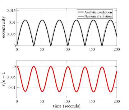
Figure 1: Evolution of the eccentricity (black) and relative change in the separation (red) over several (phase-matched) relaxed orbits for a quasi-circular pair of solar mass white dwarfs (both with radii $6\times 10^{6}$ m) with orbital frequency 30 mHz (periastron separation $3.3R_{1}$).

for a quasi-circular pair of solar mass white dwarfs with orbital frequency 30 mHz. The numerical solution has been artificially damped by including the term $-\dot{b}_{\bf k}/\tau_{d}$ in (14), where $\tau_{d}=\tau_{d}^{(0)}{\rm e}^{t/\tau_{d}^{(0)}}$ with $\tau_{d}^{(0)}=10^{4}\,\mathrm{s}$. This introduces a phase lag which we have corrected for in the figure. A 4th-order Runge-Kutta integrator was used to obtain the numerical solution. Also shown is the time dependence of the distance between the stars, given to first-order in eccentricity for a quasi-circular orbit by

$$\begin{split}r(t)&=a(1-e\cos M)\\ &=a\left[1-\frac{1}{2}\left(z^{*}{\rm e}^{i\lambda}+z{\rm e}^{-i\lambda}\right)\right]\\ &=a\left[1-2A_{\rm tot}\sin^{2}(\nu t/2)\right]\end{split}$$ (25)

Thus the orbit is truly non-circular as long as the dynamical tide operates. The amplitude of the effect will be modified by tidal friction and gravitational wave emission and will tend towards a perfectly circular orbit as the oscillations cease (for example, when the spins are perfectly synchronous in the absence of accretion); this will be addressed in a companion paper.

2.3 The apsidal motion constant

The quadrupole apsidal motion constant of an object, $k_{2}^{(1)}$, is defined to be such that the quadrupole contribution to the perturbing potential due to its non-sphericity (itself induced by a companion body of mass $m_{2}$ and distance $a$, and/or spin distortion) is (Sterne, 1939)

$$\Phi_{\rm quad}=\frac{Gm_{2}}{R_{1}}\left(\frac{R_{1}}{a}\right)^{6}(2k_{2}^{(1)}).$$ (26)

Substituting (16) into (13), retaining zeroth-order terms in eccentricity and quadrupole terms only and taking the system to be far from resonance (ie, ignoring the contribution $4\overline{\nu}^{2}$ to the denominator), (13) divided by $m_{1}$ becomes

$$\frac{{\cal R}_{\rm tide}}{m_{1}}\simeq\frac{Gm_{2}}{R_{1}}\left(\frac{R_{1}}{a}\right)^{6}\left(\frac{4\pi}{5}\frac{T_{12}^{2}}{I_{k\!l}\overline{\omega}_{12}^{2}}\right).$$ (27)

Comparing this to (26) gives

$$k_{2}^{(1)}=\frac{2\pi}{5}\frac{T_{12}^{2}}{I_{12}\overline{\omega}_{12}^{2}}=\frac{2\pi}{5}\left(\frac{Q_{12}}{\overline{\omega}_{12}}\right)^{2},$$ (28)

so that from Table 1 for an $n=1.5$ polytrope we obtain $k_{2}^{(1)}=0.143$, which compares favourably to Stern’s value of 0.145. We also have that for systems far from resonance, the variation of the eccentricity due to tidal distortion is such that

$$A_{12}\simeq 6k_{2}^{(1)}\left(\frac{m_{2}}{m_{1}}\right)\left(\frac{R_{1}}{a}\right)^{5}.$$ (29)

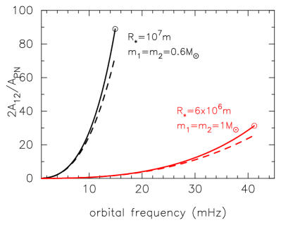
Figure 2: Relative strength of contribution to eccentricity amplitude from tides and relativity as a function of orbital frequency for two different white dwarf pairs. The dashed curves use the approximation (29) for $A_{12}$ and demonstrate that a measurement of $A_{\rm tot}$ usefully constrains the apsidal motion constant $k_{2}^{(1)}$ for detectable binaries. The circles at the end of the curves indicate Roche contact.

Figure 2 shows the relative strength of the contributions to the eccentricity amplitude from tides and relativity as a function of orbital frequency for white dwarf pairs with $m_{1}=m_{2}=0.6M_{\odot}$, $R_{1}=R_{2}=10^{9}\,{\rm cm}$ (black curves) and $m_{1}=m_{2}=1.0M_{\odot}$, $R_{1}=R_{2}=6\times 10^{8}\,{\rm cm}$ (red curves). The dashed curves use the approximation (29) for $A_{12}$ and demonstrate that a measurement of $A_{\rm tot}$ usefully constrains internal structure information, especially if the chirp mass can be measured (Section 2.4) and electromagnetic follow-up observations can be done. In practice, a measurement of the ratio of the strains at the $n=3$ (and/or the $n=1$) and $n=2$ harmonics constrains the quantity

$$6\left[k_{2}^{(1)}\left(\frac{m_{2}}{m_{1}}\right)\left(\frac{R_{1}}{a}\right)^{5}+k_{2}^{(2)}\left(\frac{m_{1}}{m_{2}}\right)\left(\frac{R_{2}}{a}\right)^{5}\right]-\left(3-\eta\right)\left(\frac{a\nu}{c}\right)^{2},$$ (30)

where $R_{1}$, $R_{2}$ and $k_{2}^{(1)}$, $k_{2}^{(2)}$ are the radii and apsidal motion constants of stars 1 and 2 respectively.

2.4 Dissipation and chirp

Resolvable quasi-circular white dwarf binaries in the LISA/DECIGO/BBO frequency band will have orbital periods in the range $3-50\,{\rm mHz}$, with the upper bound corresponding to Roche contact of two stars at the Chandrasekhar mass limit (Eggleton, 1983). Such an orbit will decay slightly during the observing period as a result of gravitational wave emission and tidal friction. The associated timescales for change in the orbital frequency, $\tau_{\rm GR}$ and $\tau_{\rm tides}$, are such that (Peters, 1964)

$$\tau_{\rm GR}^{-1}=\frac{96}{5}\nu\eta\left(\frac{a\nu}{c}\right)^{5}\left(1+\frac{157}{24}\langle e^{2}\rangle\right)$$ (31)

and (Mardling & Lin, 2002, equation (55))

$$\begin{split}\tau_{\rm tides}^{-1}&=\frac{171}{4}\nu\left[\left(\frac{k_{2}^{(1)}}{Q_{1}}\right)\left(\frac{m_{2}}{m_{1}}\right)\left(\frac{R_{1}}{a}\right)^{5}+\left(\frac{k_{2}^{(2)}}{Q_{2}}\right)\left(\frac{m_{1}}{m_{2}}\right)\left(\frac{R_{2}}{a}\right)^{5}\right]\langle e^{2}\rangle\\ &=\frac{57}{4}\nu\left[\frac{A_{12}^{(1)}}{Q_{1}}+\frac{A_{12}^{(2)}}{Q_{2}}\right]A_{\rm tot}^{2},\end{split}$$ (32)

where $Q_{1}$ and $Q_{2}$ are the tidal quality factors ($Q$-values) of stars 1 and 2 respectively, and $\langle e^{2}\rangle=2A_{\rm tot}^{2}$ is the time averaged value of the square of the eccentricity with $A_{\rm tot}=A_{12}^{(1)}+A_{12}^{(2)}-A_{\rm PN}$. Note that the form of (32) assumes synchronous rotation of both bodies; this will be slightly modified for asynchronous rotation. The chirp timescale, $\tau_{\nu}$, is then such that

$$\tau_{\nu}^{-1}=\tau_{\rm GR}^{-1}+\tau_{\rm tides}^{-1},$$ (33)

so that over an observing time $T$, the chirp, $\Delta f_{b}$, is given by

$$\frac{\Delta f_{b}}{f_{b}}=\frac{T}{\tau_{\nu}},$$ (34)

where $f_{b}=\nu/2\pi$ is the orbital cyclic frequency.

Taking $Q_{1}=Q_{2}=10^{7}$ (Burkart et al., 2013), orbital decay is completely dominated by gravitational wave emission for all white dwarf binaries up to Roche contact, at which point $\tau_{\rm tides}/\tau_{\rm GR}$ has reduced to 3400 and 200 for $1.0\,M_{\odot}$ and $0.6\,M_{\odot}$ pairs respectively. Taking $\tau_{\nu}\simeq\tau_{\rm GR}$ one can then write

$$\frac{\Delta f_{b}}{f_{b}}\simeq\frac{T}{100\,{\rm yr}}\left(\frac{\cal M}{M_{\odot}}\right)^{5/3}\left(\frac{f_{b}}{30\,{\rm mHz}}\right)^{8/3},$$ (35)

where

$${\cal M}=\frac{(m_{1}m_{2})^{3/5}}{(m_{1}+m_{2})^{1/5}}=\eta^{3/5}(m_{1}+m_{2})$$ (36)

is the chirp mass, so that a measurement of the chirp allows one to estimate ${\cal M}$ if the signal to noise is adequate. The range of $\tau_{\nu}$ for a pair of solar mass white dwarfs is 58,480 yr at 3 mHz to 59 yr at 40 mHz (Roche contact), with the corresponding chirp over 5 years of 0.003 and $3.4\,{\rm mHz}$ respectively, or double these for the prominent $n=2$ harmonic. For a pair of $0.6\,M_{\odot}$ white dwarfs the range is 137,012 yr at 3 mHz to 1874 yr at 15 mHz (Roche contact), with corresponding chirp of $10^{-4}-0.04\,{\rm mHz}$.

Note that white dwarf binaries close to or at contact are likely to involve some angular momentum loss from the system via mass loss, in which case the chirp will larger than predicted by (35) (see Section 3.5).

3 Impact on the gravitational wave signal

The dimensionless gravitational wave strain tensor is given by Einstein’s quadrupole formula

$$h_{i\!j}=\frac{2G}{c^{4}D}\Lambda_{i\!j,k\!l}\ddot{\cal I}^{k\!l}=2\eta\left(\frac{a}{D}\right)\left(\frac{a\nu}{c}\right)^{4}\Lambda_{i\!j,k\!l}\left(\frac{\ddot{\cal I}^{k\!l}}{\mu a^{2}\nu^{2}}\right),$$ (37)

where ${\cal I}^{k\!l}$ is the (symmetric) moment of inertia tensor of the object emitting the gravitational waves, $D$ is its distance from the observer, and $\Lambda_{i\!j,k\!l}$ is a sky-projection operator which selects the transverse trace-less part of ${\cal I}^{k\!l}$ (Maggiore, 2007). Then

$$[h_{i\!j}]=\left[\begin{array}[]{ccc}h_{+}&h_{\times}&0\\ h_{\times}&-h_{+}&0\\ 0&0&0\end{array}\right],$$ (38)

where

$$h_{+}=\frac{1}{2}h_{0}(\ddot{\cal I}^{11}-\ddot{\cal I}^{22})/(\mu a^{2}\nu^{2})$$ (39)

and

$$h_{\times}=h_{0}\ddot{I}^{12}=h_{0}\ddot{\cal I}^{21}/(\mu a^{2}\nu^{2}),$$ (40)

with $h_{0}=2\eta\left(a/D\right)\left(a\nu/c\right)^{4}$. The moment of inertia tensor for a binary star system is

$${\cal I}^{i\!j}=\mu x^{i}x^{j},$$ (41)

where $x^{i}$ are the components of the vector ${\bf r}$ giving the position of $m_{2}$ relative to $m_{1}$, and $r=|{\bf r}|$. Taking the binary to be face-on to the observer, we can write

$${\bf r}=r(\cos\psi{\bf i}+\sin\psi{\bf j}),$$ (42)

where ${\bf i}$ and ${\bf j}$ are basis vectors in the plane of the sky and $\psi$ is the true longitude measured from the ${\bf i}$ direction. The moment of inertia tensor is then

$$[{\cal I}^{i\!j}]=\mu r^{2}\left[\begin{array}[]{ccc}\cos^{2}\psi&\sin\psi\cos\psi&0\\ \sin\psi\cos\psi&\sin^{2}\psi&0\\ 0&0&0\end{array}\right]$$ (43)

so that

$$h_{+}=h_{0}\left[(\dot{r}^{2}+r\ddot{r}-2r^{2}\dot{\psi}^{2})\mathrm{cos}2\psi-(4r\dot{r}\dot{\psi}+r^{2}\ddot{\psi})\mathrm{sin}2\psi\right]/(a^{2}\nu^{2})$$ (44)

and

$$h_{\times}=h_{0}\left[(\dot{r}^{2}+r\ddot{r}-2r^{2}\dot{\psi}^{2})\mathrm{sin}2\psi+(4r\dot{r}\dot{\psi}+r^{2}\ddot{\psi})\mathrm{cos}2\psi\right]/(a^{2}\nu^{2}).$$ (45)

To first-order in the eccentricity (and hence $z$ and $z^{*}$) we can write (Murray & Dermott, 2000)

$$r/a=1-e\cos(\lambda-\varpi)=1-\frac{1}{2}\left(z^{*}{\rm e}^{i\lambda}+z{\rm e}^{-i\lambda}\right),$$ (46)

and

$$\psi=\lambda+2e\sin(\lambda-\varpi)=\lambda-i\left(z^{*}{\rm e}^{i\lambda}-z{\rm e}^{-i\lambda}\right).$$ (47)

The time derivatives of $r$ and $\psi$ are obtained with $z(t)$ given by (19), and (44) and (45) can be expanded to first order in $A_{\rm tot}$ to give

$$\begin{split}h_{+}(t)&=h_{0}\left[(-4+8A_{\rm tot}^{(0)})\cos(2\nu t+2\lambda(0))\right.\\ &\left.-3A_{\rm tot}^{(0)}\cos(\nu t+2\lambda(0))+9A_{\rm tot}^{(0)}\cos(3\nu t+2\lambda(0))\right]\end{split}$$ (48)

and

$$\begin{split}h_{\times}(t)&=h_{0}\left[(-4+8A_{\rm tot}^{(0)})\sin(2\nu t+2\lambda(0))\right.\\ &\left.-3A_{\rm tot}\sin(\nu t+2\lambda(0))+9A_{\rm tot}^{(0)}\sin(3\nu t+2\lambda(0))\right].\end{split}$$ (49)

3.1 Waveform in frequency space

In order to assess the detectability of various harmonics in the gravitational wave signal, we consider the signal in the frequency domain by calculating the discrete Fourier transform (DFT) of the strain, which for the $k$th frequency bin is

$${h}(f_{k})=\frac{1}{N}\sum_{n=1}^{N}h_{\times}(t_{n})e^{2\pi if_{k}t_{n}}=\frac{1}{N}\sum_{n=1}^{N}h_{\times}(t_{n})e^{2\pi ikn/N},$$ (50)

where $N$ is the number of points in the data stream and $h_{\times}(t_{n})$ the strain at time $t_{n}=nT/N$. Note that any normalised linear combination of $h_{+}$ and $h_{\times}$ in (50) will yield the same results for the amplitude spectral density (ASD). For a sampling frequency of $1\,\mathrm{Hz}$ and an observing time $T$ of 5 years, the frequency resolution of the data stream, $\Delta f=1/T$, is $6\times 10^{-9}\,{\rm Hz}$. The ASD of the (Fourier transformed) signal $h(f_{k})$ is then

$$\tilde{h}(f_{k})=\sqrt{\frac{|{h}(f_{k})|^{2}}{\Delta f}}=|{h}(f_{k})|\sqrt{T},$$ (51)

which can be compared to the detector noise as follows.

Using an optimal matched filter, the signal-to-noise ratio, $\mathcal{S}/\mathcal{N}$, of a continuous signal $h_{\times}(t)$, whose continuous Fourier transform is $H(f)$ (units Hz^-1), is given by (Flanagan & Hughes, 1998)

$$(\mathcal{S}/\mathcal{N})^{2}=4\int_{0}^{\infty}\mathrm{d}f\frac{|H(f)|^{2}}{S(f)},$$ (52)

where $S(f)$ is the noise power spectral density (units Hz^-1). For a discrete data stream and with our definition (50) of the DFT, the signal-to-noise ratio is instead given by (Moore et al., 2015)

$$(\mathcal{S}/\mathcal{N})^{2}=4\sum_{k=0}^{N-1}\frac{|\tilde{h}(f_{k})|^{2}}{S_{k}(f)}=4T\sum_{k=0}^{N-1}\frac{|{h}(f_{k})|^{2}}{S_{k}(f)}.$$ (53)

If we disregard the shrinking of the orbit due to the radiation reaction term, one can calculate the ASD (and hence the detectability of the individual harmonics) analytically from Equations (48) and (49). For each of the harmonics, the power will be concentrated in a single frequency bin, with an ASD of $|4-8A_{\rm tot}|h_{0}\sqrt{T}$ for the second harmonic, $3A_{\rm tot}h_{0}\sqrt{T}$ for the first harmonic, and $9A_{\rm tot}h_{0}\sqrt{T}$ for the third harmonic. Hence the signal-to-noise ratio is $\mathcal{S}/\mathcal{N}=|4-8A_{\rm tot}|h_{0}\sqrt{T/S(2f_{b})}$ for the detection of the second harmonic as an individual waveform component, and similarly for the other two harmonics.

In reality, the decay of the orbit will introduce a chirp in the waveform and broaden the spectrum slightly. However, the signal-to-noise ratio is not affected by this chirp (as long as the exact waveform is still available for constructing the optimal Wiener filter): in contrast with the late inspiral phase of neutron star and black hole binaries as observed by Advanced LIGO and VIRGO, the broadening of the individual harmonics is still small, so that for a waveform with a single harmonic at frequency $nf_{b}$, $n=1,2,3$, we obtain

$$(\mathcal{S}/\mathcal{N})_{\mathrm{chirp}}^{2}=4\int\mathrm{d}f\frac{|H_{\mathrm{chirp}}(f)|^{2}}{S(f)}\approx\frac{4}{S(nf_{b})}\int\mathrm{d}f|H_{\mathrm{chirp}}(f)|^{2}$$ (54)

for signal-to-noise $(\mathcal{S}/\mathcal{N})_{\mathrm{chirp}}^{2}$ of the chirping waveform, since the detector noise does not vary appreciably over the frequency range traversed by the chirping binary. Here $H_{\mathrm{chirp}}(f)$ is the continuous Fourier transform of (49) with $\nu t$ replaced by $\nu_{0}t+\frac{1}{2}t^{2}/\tau_{\nu}$, where $\nu_{0}$ is the initial orbital frequency and $\tau_{\nu}$ is given in (33), yielding

$$H_{\rm chirp}(f)=\frac{h_{0}}{2}\left[(-4+8A_{\rm tot}){\cal I}_{2}(f)-3A_{\rm tot}{\cal I}_{1}(f)+9A_{\rm tot}{\cal I}_{3}(f)\right],$$ (55)

with

$${\cal I}_{n}(f)=\left\{\begin{array}[]{ll}\displaystyle{\left(\frac{\tau_{\nu}}{T}\right)\sqrt{\frac{1}{2nf_{b}\tau_{\nu}}}{\rm e}^{-i\phi_{n}}},&a_{n}(f)b_{n}(f)<0,\\ &\\ 0,&a_{n}(f)b_{n}(f)\geq 0,\end{array}\right.$$ (56)

$$a_{n}(f)=-\left(f/f_{b}-n\right),\hskip 14.22636ptb_{n}(f)=nT/\tau_{\nu}-(f/f_{b}-n),$$ (57)

and

$$\phi_{n}=(\pi f_{0}\tau_{\nu}/n)(f/f_{0}-n)^{2}+\pi/4.$$ (58)

Here we have used the method of stationary phase to evaluate the integrals associated with the damping term. The approximation used picks up the box-like structure of the chirp, correctly giving its maximum value and width but not producing the splayed structure at low ASD. Thus, the signal-to-noise only depends on the total power in the harmonic, which can also be computed from the waveform in the time domain by dint of Parseval’s theorem,

$$(\mathcal{S}/\mathcal{N})_{\mathrm{chirp}}^{2}=\frac{1}{\pi S(nf_{b})}\int\mathrm{d}t|h_{\mathrm{chirp}}(t)|^{2}=\frac{T\langle|h_{\mathrm{chirp}}(t)|^{2}\rangle}{\pi S(nf_{b})}.$$ (59)

Since the change in orbital separation over realistic integration periods is small, the mean-square average $\langle|h_{\mathrm{chirp}}(t)|^{2}\rangle$ of the strain is essentially the same with and without the radiation reaction term. The case of several discrete harmonics is no different, and we can therefore work directly with the amplitudes from Equations (48) and (49) to assess the detectability of the individual harmonics. As such, we define the “effective ASD” as the ASD without chirp, and use this to assess the signal-to-noise ratio of a detection.

Figure 3

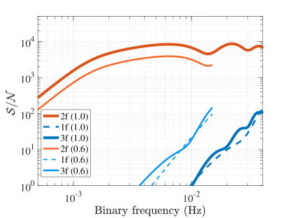
Figure 3: Signal-to-noise ratio (calculated using the “effective ASD”) as a function of binary frequency up to Roche contact for second (red), third (solid blue) and first (dashed blue) orbital harmonics, for a pair of $1\,M_{\odot}$ white dwarfs with radii $6\times 10^{8}\,{\rm cm}$ (thick lines), and a pair of $0.6\,M_{\odot}$ white dwarfs with radii $10^{9}\,{\rm cm}$ (thin lines). A distance of 1 kpc is assumed together with an integration time of 5 yr. The tidally induced first and third harmonics rise above a LISA detection threshold of 8 at orbital frequencies 15 mHz and 7 mHz respectively.

shows the signal-to-noise ratio as a function of binary frequency up to Roche contact for the first three harmonics associated with a pair of $1\,M_{\odot}$ white dwarfs with radii $6\times 10^{8}\,{\rm cm}$ (thick lines), and a pair of $0.6\,M_{\odot}$ white dwarfs with radii $10^{9}\,{\rm cm}$ (thin lines) (Sections 3.3 and 3.4). A distance of 1 kpc is assumed together with an integration time of 5 yr. The tidally induced first and third harmonics rise above a LISA detection threshold of 8 at orbital frequencies 15 mHz and 7 mHz respectively. Both cases are plotted up to Roche contact.

3.2 Matched filter templates

Equation (55) shows that for a given observing time $T$, templates for the three-harmonic box-like spectra described here involve 4 free parameters: the orbital frequency $f_{b}$, the amplitudes of the $n=2$ and 3 harmonics and the width of $n=2$ (or $n=3$) harmonic. These in turn can be used to solve for $h_{0}$, $A_{\rm tot}$ and $\tau_{\nu}$. The minimum requirement for $\tau_{\nu}$ to be measurable is that $nT/\tau_{\nu}>\Delta f/f_{b}$, where again $\Delta f$ is the frequency resolution given by the sampling rate over the observing time (see equation (57)), that is, a finite chirp width must be measurable for one of the harmonics. Thus according to equation (35), in the case that $\tau_{\nu}$ is dominated by gravitational wave emission and for a sampling frequency of 1 Hz and an observing baseline of 5 years, the chirp of the $n=2$ harmonic is (in principle) measurable if the orbital frequency is greater than 0.5 mHz. If the chirp cannot be measured, only $A_{\rm tot}$ and the combination $h_{0}\sqrt{\tau_{\nu}}$ can be solved for.

Finally, note that while the amplitudes are affected by chirp (whether or not it can be measured), the ratio of amplitudes is not.

3.3 Signal from a high–mass 30 mHz quasi–circular binary

Figure 4

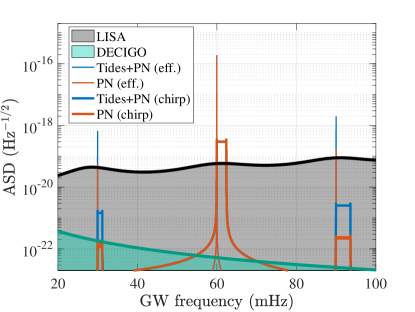
Figure 4: The ASD (with chirp: box-like structures) and “effective ASD” (no chirp: individual spikes) for a quasi-circular pair of $1\,M_{\odot}$ cold white dwarfs with orbital frequency 30 mHz, radii $6\times 10^{8}\,{\rm cm}$, at a distance of 1 kpc and for 5 years of detector integration. Red indicates the signal with PN terms only, while blue includes both tides and GR. Since the chirp is small, the signal-to-noise of the true chirping signal (using the analytical form (55) as a template) is effectively the same as that for the signal with no chirp, allowing one to use the effective ASD to estimate this quantity. Relative to the LISA noise ASD we obtain $\mathcal{S}/\mathcal{N}$ ratios of 30, 6000 and 40 for the $n=1,2,3$ harmonics respectively, making the tidal contribution to the signal resolvable and loud for LISA. See text for details.

shows the amplitude spectral density for a quasi-circular pair of $1\,M_{\odot}$ cold white dwarfs with orbital frequency 30 mHz, radii $6\times 10^{8}\,{\rm cm}$ (Timmes, 2014), at a distance of 1 kpc and for 5 years of detector integration. The signal is plotted with and without chirp: the box-like structures are with chirp, while the single spikes are without and indicate the “effective ASD”. Red is used for the signal without tides (but including the post-Newtonian correction), while blue includes both tides and PN. The curved structures visible around $60\,{\rm mHz}$ are a result of using a discrete Fourier transform, here calculated using a Fast Fourier Transform routine; the analytic forms for both the chirped (equation (55)) and non-chirped (paragraph following eqn. (53)) signals accurately predict the amplitudes, without the (irrelevant) curved structures. Also shown is the LISA sensitivity ASD (Larson et al., 2000) (black/grey) which is based on five years of observation, as well as the DECIGO noise (green; Yagi & Seto, 2011). Note that for this system the orbital separation is $a=3.26R_{*}$, thereby avoiding Roche contact by 23% (Eggleton, 1983), while the orbital decay timescale due to radiation reaction is 125 yr (Peters, 1964),

yielding a chirp of $2.4\,{\rm mHz}$ for the $n=2$ harmonic over the 5 years.

Assuming an optimal matched filter, the signal-to-noise ratio of each harmonic can be estimated using the excess of effective ASD over the noise floor, multiplied by a factor of 2 (equation (52) or (53)). For LISA we obtain ${\cal S}/{\cal N}=30$, 6000 and 40 for the $n=1,2,3$ harmonics respectively, while for DECIGO the corresponding values are 6000, $8\times 10^{6}$ and $2\times 10^{5}$. Since no foreground strain from Galactic white dwarf pairs is expected at these frequencies (Ruiter et al., 2010; Bender, 1998), such a signal should be resolvable and loud for LISA at 1 kpc, while DECIGO will be able to detect it at Mpc scales.

Consistent with Figure 2, tidal distortion clearly dominates the PN contribution to the signal at the $n=1$ and 3 harmonics, providing a valuable constraint on the internal structure of the stars, especially if the system is close enough to follow up with spectroscopic and/or photometric observations. Note from Fig. 2 that resonant forcing of the quadrupole $f$-mode is not significant.

3.4 Signal from a $0.6\,M_{\odot}$ pair at 15 mHz

Figure 5

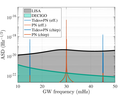
Figure 5: Same as Fig. 4 but for a quasi-circular pair of $0.6M_{\odot}$ white dwarfs with orbital frequency 15 mHz, radii $10^{9}\,{\rm cm}$, again at a distance of 1 kpc and for 5 years of detector integration. Relative to the LISA noise ASD, the signal-to-noise ratios are 80, 2300 and 130 for the $n=1,2,3$ harmonics respectively, again making the tidal contribution to the signal resolvable and loud for LISA.

shows the true and effective ASD for a quasi-circular pair of $0.6\,M_{\odot}$ white dwarfs with orbital frequency 15 mHz, radii $10^{9}\,{\rm cm}$, and again at a distance of $1\,\mathrm{kpc}$ and for 5 years of detector integration. Such a binary is close to filling its Roche lobe (see Fig. 2), and has a coalescence timescale of 1866 yr. While the chirp is small at 0.1 mHz for the $n=2$ harmonic, it significantly reduces the peak amplitudes of the three harmonics, making it vital to use the chirped waveform (55) as a template in any optimal matched filter search. For this system, ${\cal S}/{\cal N}=80$, 2300 and 130 for the $n=1,2,3$ harmonics respectively for LISA, making the source detectable at distances up to several kpc, while for DECIGO the corresponding values are 2000, $5\times 10^{5}$ and $4\times 10^{4}$, again making the system detectable at Mpc scales.

For this generic pair of white dwarfs, the tides again clearly dominate the PN contribution to the signal at the $n=1$ and 3 harmonics. Note again from Fig. 2 that resonant forcing of the quadrupole $f$-mode is not significant.

3.5 Signal from the cataclysmic variable HM Cnc at 3 mHz

HM Cnc (RX J0806.3+1527) is a cataclysmic variable with an orbital period of 5.4 min (3.1 mHz), making it the shortest-period binary star known (Barros et al., 2007) and therefore one of the strongest “verification sources” of gravitational waves for LISA (Roelofs et al., 2010). It consists of a white dwarf accreting from a less massive second white dwarf, with relative radial velocity measurements providing a mass ratio estimate of $0.50\pm 0.13$ (Roelofs et al., 2010), and with upper limits on the masses of the individual components of $0.9\,M_{\odot}$ and $0.45\,M_{\odot}$ (Barros et al., 2007). Roelofs et al. (2010) finds that the orbital frequency must be adjusted by $3.57\times 10^{-16}\,{\rm Hz\,s}^{-1}$ in order to improve the accuracy of the ephemeris over three years; this corresponds to masses of $0.54\,M_{\odot}$ and $0.27\,M_{\odot}$ if the frequency is modulated by gravitational wave emission alone. We adopt these masses here.

Excitation of the $n=1$ and 3 harmonics of the orbital period will persist for semi-detached and contact systems. Figure 6

Figure 6: Effective ASD after 5 years of integration for the verification system HM Cnc, a 3.1 mHz cataclysmic variable consisting of a white dwarf accreting from a companion white dwarf half its mass. Assuming a quasi-circular orbit, parameters adopted are $m_{1}=0.27\,M_{\odot}$, $m_{2}=0.54\,M_{\odot}$, $R_{1}=2.1\times 10^{9}$ cm (the Roche radius for this observationally determined mass ratio and period and adopted masses), and $D=1$ kpc. Also shown is the foreground confusion limit adapted from Ruiter et al. (2010) Fig. 10 (light green curve), which drops below the LISA noise floor at around 6 mHz. With a signal-to-noise of 20, the $n=3$ harmonic should be detectable at this distance.

shows the expected signal after 5 years of integration for donor and accretor masses of $0.27\,M_{\odot}$ and $0.54\,M_{\odot}$ respectively, donor radius of $R_{1}=2.1\times 10^{9}$ cm (the Roche radius for this observationally determined mass ratio and period, assuming the adopted masses), and distance 1 kpc. A quasi-circular orbit is assumed. Also shown is the foreground confusion limit (light green curve) adapted from Ruiter et al. (2010) Fig. 10, showing that the foreground no longer dominates the noise around 6 mHz (black curve). With a signal-to-noise of 20, the $n=3$ harmonic should be detectable at this distance, as it should be up to a distance of 2.3 kpc for a signal-detection limit of 8. Note that over a 5 year observing period, the chirp is 56 nHz from GR alone, which is greater than the frequency resolution $\Delta f$. The true signal therefore has finite width, and the resulting reduction in amplitude (compared to the effective ASD) is shown in the Figure.

Note that the chirp will be modified by mass transfer, which may well be non-conservative. In fact the X-ray luminosity of this system is significantly lower than expected for a system in which mass-transfer is driven by gravitational radiation, and a possible way to reconcile this is if the system is losing angular momentum through mass loss (Willems & Kalogera, 2005).

Note also that HM Cnc displays X-ray and optical light-curve modulations at the orbital period which are consistent with eccentricity of the order of 0.1 (Mardling, in preparation); if this is the case and the $n=3$ harmonic is detectable, its amplitude relative to that of the $n=2$ harmonic will be larger than shown here, and given the observational constraints on the masses, can be used to constrain the eccentricity according to our analysis (equation (18) with $e(0)>0$). We will generalize our analysis to arbitrary eccentricity in a future publication.

Finally, note that due to the relatively large radius of the Roche-filling star, the tidal contribution to the gravitational wave signal from the $n=1$ and 3 harmonics is more than 100 times that of the general relativistic contribution.

4 Summary and discussion

Using the formalism of Gingold & Monaghan (1980) for the self-consistent treatment of the interaction between a binary orbit and the dynamical tide of a non-rotating star, we have demonstrated that as long as the stars oscillate, the osculating eccentricity will be non-zero and the orbit will be non-circular as we show in equation (25) and Figure 1. Here we have only included the dominant quadrupole $f$-mode, neglecting any resonances that may exist with lower-frequency $g$-modes.

A small time-varying eccentricity produces gravitational wave power at the first and third harmonics of the binary frequency, in addition to the usual power in the second harmonic. The result is important because it provides access to knowledge of the internal structure of the stars, with the amplitude of the $n=1$ and 3 harmonics being proportional to the induced eccentricity, which itself depends linearly on the apsidal motion constants of the stars. Thus, in contrast to the classical technique used to determine these quantities (eg. Claret & Giménez, 2010), our approach does not necessitate the measurement of the rate of apsidal advance, and complements asteroseismological studies of pulsating white dwarfs (Winget & Kepler, 2008). See also Seto (2001) and Willems et al. (2008) for the effect of apsidal advance on gravitational wave signals from binaries, and Batygin et al. (2009) and Mardling (2010) for a description of how the apsidal motion constant of a hot Jupiter can be determined without measuring the apsidal motion rate.

Close binaries are expected to tidally circularize on a timescale which depends on the mass ratio, the ratio of the stellar radius to the stellar separation, the apsidal motion constants of the stars (which themselves depend on their equations of state), and their $Q$-values which characterize the efficiency at which they dissipate the tidal motion. We have assumed that the short-period systems considered here are in the relaxed quasi-circular state, with the corresponding gravitational wave signal depending on this assumption. However, it is not known how mass loss affects the orbital evolution, and there is reason to believe that semi-detached systems such as the LISA verification binary HM Cnc are not fully circularized (Mardling, in preparation). If this is indeed the case, it should be evident in the ratio of amplitudes of the $n=2$ and 3 harmonics, and in the frequency-splitting effect of the associated apsidal advance as described in Willems et al. (2008).

Another consequence of tidal evolution is spin synchronization and alignment. While our analysis does not include the influence of spin on the gravitational wave signal, one effect will be to contribute an additional quadrupole potential due to spin distortion, modifying slightly the harmonic amplitudes. Note that systems for which the spin synchronization timescale is longer than the orbital shrinkage timescale are not expected to actually achieve the synchronous state (Fuller & Lai, 2012), although it is likely to be close unless some kind of non-1:1 Cassini state is established which may happen if the eccentricity is significant and the equation of state is appropriate as is the case for Mercury in the Solar System (eg. Correia, 2015).

We have shown that the gravitational wave amplitudes for the $n=1$ and 3 harmonics are dominated by the tidal contribution to the potential, with the relativistic contribution at least an order of magnitude less for systems for which the these harmonics are detectable. In addition we have shown that the orbital frequencies of white dwarf binaries remain far from resonance with the dominant $f$-mode, all the way to Roche contact. As such, a measurement of the ratio of amplitudes of the $n=2$ and 3 harmonics corresponds to a measurement of the combination of parameters given in (30), thereby placing useful constraints on the apsidal motion constants of the stars, especially if the masses and radii are available from standard spectroscopy and photometry as is the case for HM Cnc.

In spite of the fact that significantly non-circular short-period white dwarf binaries are expected to be extremely rare in the Galaxy, significant effort has been spent on calculating their gravitational wave signal (eg. Pierro et al., 2001; Willems et al., 2007). While the dense stellar environments in which such binaries form promote the formation of highly eccentric binaries, and indeed excite the eccentricities of tidally relaxed binaries through multiple encounters, in the end it is a contest between the circularization timescale and the encounter timescale, with the former almost certainly winning in most cases. On the other hand, while the vast majority of close binary white dwarfs are isolated in the field and are therefore expected to be circular, the work described here offers the chance to test this assumption using the new frontier of gravitational wave astronomy.

99

Appendix A The rate of change of $z=e{\rm e}^{i\varpi}$

In the case that the perturbing acceleration can be written in terms of the gradient of a potential, one can use Lagrange’s planetary equations (eg. Murray & Dermott, 2000) to write

$$\dot{z} = \left(\frac{\dot{e}}{e}+i\dot{\varpi}\right)z=\frac{1}{\mu\nu a^{2}e}\left(-\frac{1}{e}\frac{\partial{\cal R}}{\partial{\varpi}}+i\frac{\partial{\cal R}}{\partial{e}}\right)z.$$ (60)

Using the chain rule we have

$$\frac{\partial{\cal R}}{\partial{e}} = \frac{\partial{\cal R}}{\partial{z}}\frac{\partial{z}}{\partial{e}}+\frac{\partial{\cal R}}{\partial{z^{*}}}\frac{\partial{z^{*}}}{\partial{e}}=\frac{1}{e}\left(z\frac{\partial{\cal R}}{\partial{z}}+z^{*}\frac{\partial{\cal R}}{\partial{z^{*}}}\right)$$ (61)

and

$$\frac{\partial{\cal R}}{\partial{\varpi}} = \frac{\partial{\cal R}}{\partial{z}}\frac{\partial{z}}{\partial{\varpi}}+\frac{\partial{\cal R}}{\partial{z^{*}}}\frac{\partial{z^{*}}}{\partial{\varpi}}=i\left(z\frac{\partial{\cal R}}{\partial{z}}-z^{*}\frac{\partial{\cal R}}{\partial{z^{*}}}\right)$$ (62)

so that

$$\dot{z}=\frac{2i}{\mu\nu a^{2}}\frac{\partial{{\cal R}}}{\partial{z^{*}}}.$$ (63)

The rate of apsidal advance is then

$$\dot{\varpi}=\frac{1}{2i}\left(\frac{\dot{z}}{z}-\frac{\dot{z}^{*}}{z^{*}}\right).$$ (64)

For a general perturbing acceleration ${\bf a}$, the rate of change of $z$ can be written in terms of the Runge-Lenz vector, the latter being (eg. Mardling & Lin, 2002)

$$\dot{\bf e}=\left(2({\bf a}\cdot\dot{\bf r}){\bf r}-({\bf r}\cdot\dot{\bf r}){\bf a}-({\bf a}\cdot{\bf r})\dot{\bf r}\right)/G(m_{1}+m_{2}),$$ (65)

so that using equations (28) and (31) of Mardling & Lin (2002) with $\hat{\bf e}=\cos\varpi\,{\bf i}+\sin\varpi\,{\bf j}$ and $\hat{\bf q}=-\sin\varpi\,{\bf i}+\cos\varpi\,{\bf j}$ we have

$$\dot{z}=({\bf i}\cdot\dot{\bf e})+i\,({\bf j}\cdot\dot{\bf e}).$$ (66)

In terms of the mean anomaly $M$, to first-order in eccentricity one has

$$r=a(1-e\cos M),\hskip 14.22636pt\dot{r}=a\nu e\sin M,$$ (67)

and

$$f=M+2e\sin M,\hskip 14.22636pt\dot{f}=\nu(1+2e\cos M).$$ (68)

Putting ${\bf e}_{r}=\cos(f+\varpi){\bf i}+\sin(f+\varpi){\bf j}$, ${\bf e}_{\psi}=-\sin(f+\varpi){\bf i}+\cos(f+\varpi){\bf j}$ and $M=\lambda-\varpi$, for ${\bf a}={\bf a}_{\rm PN}$ one obtains

$$\dot{z}_{\rm PN}=i\nu\left(\frac{a\nu}{c}\right)^{2}\left[3z-(3-\eta){\rm e}^{i\lambda}-(11-6\eta)z^{*}{\rm e}^{2i\lambda}\right],$$ (69)

while for ${\bf a}=(1/\mu)\partial{\cal R}_{\rm tide}/\partial{\bf r}$ (see equation (2)) we have

$$\dot{z}_{\rm QD}=i\nu k_{2}\left(\frac{m_{2}}{m_{1}}\right)\left(\frac{R_{1}}{a}\right)^{5}\left[15z+6{\rm e}^{i\lambda}+27z^{*}{\rm e}^{2i\lambda}\right]$$ (70)

which recover (17) to zeroth-order in $z$ and $z^{*}$ (in the limit that $\nu\ll\omega_{12}$). On the other hand, orbit-averaging gives

$$\left<\dot{z}\right>=\left<\dot{z}_{\rm QD}+\dot{z}_{\rm PN}\right>=i(\dot{\varpi}^{\rm(QD)}_{\rm sec}+\dot{\varpi}^{\rm(PN)}_{\rm sec})z,$$ (71)

where

$$\dot{\varpi}^{\rm(QD)}_{\rm sec}=3\nu\left(\frac{a\nu}{c}\right)^{2}\hskip 8.5359pt{\rm and}\hskip 8.5359pt\dot{\varpi}^{\rm(PN)}_{\rm sec}=15\nu k_{2}\left(\frac{m_{2}}{m_{1}}\right)\left(\frac{R_{1}}{a}\right)^{5}$$ (72)

are the standard expressions for the secular rate of apsidal advance due to the tidal quadrupole distortion and post-Newtonian acceleration (eg. Sterne, 1939; Mardling & Lin, 2002), so that from (64),

$$\dot{\varpi}_{\rm sec}=\dot{\varpi}^{\rm(QD)}_{\rm sec}+\dot{\varpi}^{\rm(PN)}_{\rm sec}.$$ (73)

Note that since integrating (71) gives

$$z(t)=z(0){\rm e}^{i\dot{\varpi}_{\rm sec}t},$$ (74)

there is no secular variation associated with quasi-circular orbits (for which $z(0)=0$).

Table 3: Notation

Symbol	Definition	Reference/definition
$A_{12}$	Tidal contribution to eccentricity amplitude	Eq. (20)
$A_{\mathrm{PN}}$	Post-Newtonian contribution to eccentricity amplitude	Eq. (21)
$a$	Semi-major axis
$b_{\textbf{k}}(t)$	Oscillation amplitude	Eqs. (15) and (16)
$c_{l\!m}$	Spherical harmonic constants	$c_{20}=-\sqrt{\pi/5}$, $c_{22}=c_{2-2}=\sqrt{3\pi/10}$
$D$	Distance to binary
$e$	eccentricity
e	Runge-Lenz vector	Goldstein (1980)
$E_{\mathrm{tot}}$	Total energy of coupled orbit and oscillator	Mardling (1995a, b); Lai (1997)
$E_{\mathrm{PN}}$	Post-Newtonian energy	Kidder (1995)
$f$	True anomaly
$H$	Continuous fourier transform of signal
$h_{i\!j}$	Dimensionless gravitational wave strain tensor	Einstein (1918); Kokkotas & Schmidt (1999)
$h_{0}$	Dimensionless strain amplitude from binary at distance $D$	$h_{0}=2\eta\left(a/D\right)\left(a\nu/c\right)^{4}$
$h_{+}$	Strain in plus polarisation	Eq. (44)
$h_{\times}$	Strain in cross polarisation	Eq. (45)
$\tilde{h}$	Strain amplitude spectral density (Hz-1/2)	Eq. (51)
$I_{k\!l}$	Structure constant, dimensionless moment of inertia of eigenmode	Gingold & Monaghan (1980); Mardling (1995a)
$\mathcal{I}^{i\!j}$	Quadrupole moment tensor	Blanchet et al. (1990)
$\textbf{J}_{\mathrm{tot}}$	Total angular momentum of coupled orbit and oscillator	Mardling (1995a, b)
$\textbf{J}_{\mathrm{PN}}$	Post-Newtonian angular momentum	Kidder (1995)
$k_{2}$	Apsidal motion constant	Sterne (1939)
$k$	Mode radial order
$l$	Mode spherical harmonic degree
$m$	Mode spherical harmonic order
k	Mode number	$klm$
$m_{i}$	Mass of $i$th star
$\mathcal{M}$	Chirp mass of binary	$(m_{1}m_{2})^{3/5}/(m_{1}+m_{2})^{1/5}=\eta^{3/5}(m_{1}+m_{2})$
$M$	Mean anomaly
$Q_{i}$	Tidal quality factor ($Q$-value) for $i$th star	Piro (2011)
$Q_{k\!l}$	Overlap integral	Lee & Ostriker (1986)
$r$	Stellar separation
r	Position vector of $m_{2}$ relative to $m_{1}$
$R_{i}$	Radius of star $i$
$\mathcal{R}_{\mathrm{tide}}$	Tide–orbit interaction energy	Mardling (1995a)
$\mathcal{S}/\mathcal{N}$	Matched filer signal–to–noise ratio	Flanagan & Hughes (1998); Moore et al. (2015)
$S_{f}$	Instrumental detector noise (Hz-1)
$T_{k\!l}$	Structure constant	Mardling (1995a); Gingold & Monaghan (1980)
$T$	Observing time
$X_{n}^{-(l+1),m}(e)$	Hansen coefficient	Eq. 12, Murray & Dermott (2000)
$x_{n}^{-(l+1),m}$	Coefficient of leading order term of Hansen coefficient	Table 2, Mardling (2013)
$x^{i}$	Components of r
$z$	Complex eccentricity	$z=e{\rm e}^{i\varpi}$, Laskar et al. (2012)
$\eta$	Dimensionless symmetric mass ratio	$\eta=m_{1}m_{2}/(m_{1}+m_{2})^{2}$
$\lambda$	Mean longitude	$\lambda=M+\varpi$
$\Lambda_{i\!j,k\!l}$	Sky–projection operator	Maggiore (2007)
$\mu$	Reduced mass	$\mu=m_{1}m_{2}/(m_{1}+m_{2})$
$\nu$	Orbital frequency (rad s-1)
$\overline{\nu}$	Dimensionless orbital frequency	$\nu/(G(m_{1}+m_{2})/R_{1})^{1/2}$
$\varpi$	Longitude of periastron
$\tau_{\mathrm{tides}}$	Tidal damping timescale	Hut (1981)
$\tau_{\mathrm{GR}}$	Merger timescale from gravitational wave emission	Peters (1964)
$\tau_{\nu}$	Chirp timescale	Eq. 33
$\Phi_{\mathrm{quad}}$	Quadrupolar perturbing potential	Sterne (1939)
$\psi$	True longitude	$\psi=f+\varpi$
$\omega_{k\!l}$	Oscillation frequency of mode with triplet k
$\overline{\omega}_{k\!l}$	Dimensionless oscillation frequency	${\omega}_{k\!l}/(G(m_{1}+m_{2})/R_{1}^{3})^{1/2}$

References

- Agol et al. (2005) Agol E., Steffen J., Sari R., Clarkson W., 2005, MNRAS, 359, 567
- Barros et al. (2007) Barros S. C. C., et al., 2007, MNRAS, 374, 1334
- Batygin et al. (2009) Batygin K., Bodenheimer P., Laughlin G., 2009, ApJ, 704, L49
- Bender (1998) Bender P. e. a., 1998, LISA Pre-Phase A Report. Garching: MPQ
- Blanchet et al. (1990) Blanchet L., Damour T., Schaefer G., 1990, MNRAS, 242, 289
- Burkart et al. (2013) Burkart J., Quataert E., Arras P., Weinberg N. N., 2013, Monthly Notices of the Royal Astronomical Society, 433, 332
- Burkart et al. (2014) Burkart J., Quataert E., Arras P., 2014, MNRAS, 443, 2957
- Claret & Giménez (2010) Claret A., Giménez A., 2010, A&A, 519, A57
- Correia (2015) Correia A. C. M., 2015, A&A, 582, A69
- Eggleton (1983) Eggleton P. P., 1983, ApJ, 268, 368
- Eggleton (2011) Eggleton P., 2011, Evolutionary Processes in Binary and Multiple Stars
- Einstein (1918) Einstein A., 1918, Sitzungsberichte der Königlich Preußischen Akademie der Wissenschaften (Berlin), Seite 154-167.,
- Flanagan & Hughes (1998) Flanagan É. É., Hughes S. A., 1998, Phys. Rev. D, 57, 4535
- Fuller & Lai (2011) Fuller J., Lai D., 2011, Monthly Notices of the Royal Astronomical Society, 412, 1331
- Fuller & Lai (2012) Fuller J., Lai D., 2012, MNRAS, 421, 426
- Fuller & Lai (2014) Fuller J., Lai D., 2014, Monthly Notices of the Royal Astronomical Society, 444, 3488
- Gingold & Monaghan (1980) Gingold R. A., Monaghan J. J., 1980, MNRAS, 191, 897
- Goldstein (1980) Goldstein H., 1980, Classical mechanics, 2nd Ed.. Addison-Wesley, Reading (MA)
- Hils et al. (1990) Hils D., Bender P. L., Webbink R. F., 1990, ApJ, 360, 75
- Hut (1981) Hut P., 1981, A&A, 99, 126
- Iben & Livio (1993) Iben Jr. I., Livio M., 1993, PASP, 105, 1373
- Kawamura et al. (2006) Kawamura S., et al., 2006, Classical and Quantum Gravity, 23, S125
- Kidder (1995) Kidder L. E., 1995, Phys. Rev. D, 52, 821
- Kokkotas & Schmidt (1999) Kokkotas K. D., Schmidt B. G., 1999, Living Reviews in Relativity, 2, 2
- Kupfer et al. (2018) Kupfer T., et al., 2018, MNRAS, 480, 302
- Lai (1997) Lai D., 1997, ApJ, 490, 847
- Larson et al. (2000) Larson S. L., Hiscock W. A., Hellings R. W., 2000, Phys. Rev. D, 62, 062001
- Laskar et al. (2012) Laskar J., Boué G., Correia A. C. M., 2012, A&A, 538, A105
- Lee & Ostriker (1986) Lee H. M., Ostriker J. P., 1986, ApJ, 310, 176
- Maggiore (2007) Maggiore M., 2007, Gravitational Waves: Volume 1: Theory and Experiments. Cambridge University Press, Cambridge (UK)
- Maoz & Mannucci (2012) Maoz D., Mannucci F., 2012, Publ. Astron. Soc. Australia, 29, 447
- Mardling (1995a) Mardling R. A., 1995a, ApJ, 450, 722
- Mardling (1995b) Mardling R. A., 1995b, ApJ, 450, 732
- Mardling (2007) Mardling R. A., 2007, MNRAS, 382, 1768
- Mardling (2010) Mardling R. A., 2010, MNRAS, 407, 1048
- Mardling (2013) Mardling R. A., 2013, MNRAS, 435, 2187
- Mardling & Lin (2002) Mardling R. A., Lin D. N. C., 2002, The Astrophysical Journal, 573, 829
- Moore et al. (2015) Moore C. J., Cole R. H., Berry C. P. L., 2015, Classical and Quantum Gravity, 32, 015014
- Murray & Dermott (2000) Murray C. D., Dermott S. F., 2000, Solar System Dynamics. Cambridge University Press, Cambridge (UK)
- Nelemans et al. (2004) Nelemans G., Jonker P. G., Marsh T. R., van der Klis M., 2004, MNRAS, 348, L7
- Peters (1964) Peters P. C., 1964, Phys. Rev., 136, B1224
- Phinney (2004) Phinney E. S., 2004, NASA Mission Concept Study.
- Pierro et al. (2001) Pierro V., Pinto I. M., Spallicci A. D., Laserra E., Recano F., 2001, MNRAS, 325, 358
- Piro (2011) Piro A. L., 2011, ApJ, 740, L53
- Roelofs et al. (2010) Roelofs G. H. A., Rau A., Marsh T. R., Steeghs D., Groot P. J., Nelemans G., 2010, ApJ, 711, L138
- Ruiter et al. (2010) Ruiter A. J., Belczynski K., Benacquista M., Larson S. L., Williams G., 2010, ApJ, 717, 1006
- Seto (2001) Seto N., 2001, Physical Review Letters, 87, 251101
- Seto (2002) Seto N., 2002, MNRAS, 333, 469
- Seto et al. (2001) Seto N., Kawamura S., Nakamura T., 2001, Physical Review Letters, 87, 221103
- Sterne (1939) Sterne T. E., 1939, MNRAS, 99, 451
- Takahashi & Seto (2002) Takahashi R., Seto N., 2002, The Astrophysical Journal, 575, 1030
- Timmes (2014) Timmes F. X., 2014, Cold white dwarf models, http://cococubed.asu.edu/code_pages/coldwd.shtml
- Timpano et al. (2006) Timpano S. E., Rubbo L. J., Cornish N. J., 2006, Phys. Rev. D, 73, 122001
- Toonen et al. (2017) Toonen S., Hollands M., Gänsicke B. T., Boekholt T., 2017, A&A, 602, A16
- Vecchio & Wickham (2004) Vecchio A., Wickham E. D. L., 2004, Phys. Rev. D, 70, 082002
- Willems & Kalogera (2005) Willems B., Kalogera V., 2005, arXiv Astrophysics e-prints,
- Willems et al. (2007) Willems B., Kalogera V., Vecchio A., Ivanova N., Rasio F. A., Fregeau J. M., Belczynski K., 2007, ApJ, 665, L59
- Willems et al. (2008) Willems B., Vecchio A., Kalogera V., 2008, Phys. Rev. Lett., 100, 041102
- Willems et al. (2010) Willems B., Deloye C. J., Kalogera V., 2010, ApJ, 713, 239
- Winget & Kepler (2008) Winget D. E., Kepler S. O., 2008, ARA&A, 46, 157
- Woods et al. (2012) Woods T. E., Ivanova N., van der Sluys M. V., Chaichenets S., 2012, ApJ, 744, 12
- Yagi & Seto (2011) Yagi K., Seto N., 2011, Phys. Rev. D, 83, 044011
- Zahn (1966) Zahn J. P., 1966, Annales d’Astrophysique, 29, 313
99