Towards Interpretable Deep Neural Networks by Leveraging
Adversarial Examples

Introduction

Sometimes it is not enough for a DNN to produce an outcome. For example, in applications such as healthcare, users need to understand the rationale of the decisions. Therefore, it is imperative to develop algorithms to learn models with good interpretability (?). An important factor that leads to the lack of interpretability of DNNs is the ambiguity of neurons, where a neuron may fire for various unrelated concepts. This work aims to increase the interpretability of DNNs on the whole image space by reducing the ambiguity of neurons. In this paper, we make the following contributions:

• We propose a metric to evaluate the consistency level of neurons in a network quantitatively.

• We find that the learned features of neurons are ambiguous by leveraging adversarial examples.

• We propose to improve the consistency of neurons on adversarial example subset by an adversarial training algorithm with a consistent loss.

Figure 1: Demonstration of the ambiguity of a neuron. When showing real images only, a neuron admittedly detects a semantic meaningful concept, but there also exist samples (e.g., adversarial samples marked with blue circles) in the high dimensional space that are different from the semantic concept but cause high response of the neuron. To reduce the ambiguity of a neuron, we propose to train DNNs adversarially by introducing a consistent loss, such that the neurons are encouraged to respond to related similar concepts or a sole concept (shown as the dashed lines).

Ambiguity of neurons

As illustrated in Figure 1, a neuron fires for a set of natural images with concept parrot, but if we evaluate on some special points of images, e.g., adversarial images, this neuron will fire for images with other concepts which are far from parrot. We call the property that a neuron fires for various unrelated concepts ambiguity of a neuron and these special points of images singular points. On the other hand, if we can hardly find singular points for a neuron, we say that the neuron is consistent and call this property consistency of a neuron.

Metric

In this section, we introduce the metric to evaluate the consistency of neurons. We first define the consistency level between a neuron $n$ and a concept $c$:

$$consis(n,c) =Pr(x\,contains\,c|x\,activates\,n)$$ (1)

where $Pr$ is the probability measure of image space. The consistency metric above is related to a certain concept. To evaluate the consistency of a neuron itself, we need a concept independent metric. Considering correlation between concepts , we quantify the consistency of neurons based on WordNet (?). As demonstrated in Figure 2, we measure the distance between different classes on the WordNet tree. We define the correlation between the corresponding concepts as

$$a_{i,j}=\exp\left(-\frac{d^{2}(w_{i},w_{j})}{2\sigma^{2}}\right),$$ (2)

where $w_{i}$, $w_{j}$ are the words of the $i,j$-th classes, $d(w_{i},w_{j})$ is their WordNet tree distance, and $\sigma$ is a hyper-parameter to control the decaying rate. We form the distance matrix by collecting each pair of the corresponding classes as $\mathbf{A}=[a_{i,j}]$. We further collect $p_{i}=consis(n,c_{i})$ for all concepts $c_{i}$ into a vector $p$ and the consistency level of a neuron $n$ is quantified as following

$$consis(n) =\|\bm{p}\|_{\mathbf{A}}^{2}=\bm{p}^{T}\mathbf{A}\bm{p}$$ (3)

Similarly, we also measure the consistency level constrained on the adversarial samples, by replacing $Pr$ with $Pr_{adv}$, where $Pr_{adv}(\cdot)=Pr(\cdot|x\,is\,an\,adversarial\,sample)$.

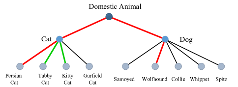
Figure 2: Illustration for quantifying the distance of different classes based on WordNet. The red path indicates the distance between persian cat and wolfhound $d=4$, which is longer than the distance between tabby cat and kitty cat ($d=2$).

Methodology

In this section, we introduce the methods. We first illustrate the inconsistency between the learned features of DNNs and semantic meaningful concepts, which motivates us to train DNNs adversarially with a consistent loss.

Inconsistency between Feature Representations and Semantic Concepts

It is a popular statement that deep visual representations have good transferability since they are disentangled (?; ?; ?). In this section, we demonstrate the weakness of this traditional view by showing that the neurons which detect high-level semantics (e.g., objects/parts) in DNNs are ambiguous.

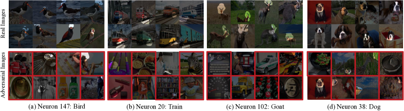
Figure 3: The real and adversarial images with highest activations for neurons in VGG-16 conv5_3 layer.

We first generate a targeted adversarial example $\bm{x}^{*}$ by solving

$$\operatorname*{arg\,min}_{\bm{x}^{*}}\|\bm{x}^{*}-\bm{x}\|_{2}+\lambda\cdot\ell(\bm{x}^{*},y^{*}).$$ (4)

We input these adversarial examples as well as the corresponding real examples into DNNs and examine their internal representations by an activation maximization method (?).

We show some visualization results in Figure 3, where the network is VGG-16 and the images are from the ImageNet dataset (?). The highlighted regions are found by discrepancy map (?). As shown in the first row of Figure 3, the neurons reveal explicit explanatory semantic meanings or human-interpretable concepts when showing real images only, but the contents of the adversarial images do not align with the semantic meanings of the corresponding neurons, if we look at the second row.

Adversarial Training with a Consistent Loss

Based on the above analysis, we propose a novel adversarial training algorithm to train DNNs for the purpose of improving the consistency of neurons. We introduce a consistent (feature matching) loss in adversarial training. Specifically, we train a DNN parameterized by $\theta$ via minimizing an adversarial objective as

$$\begin{split}\min_{\theta}L(\theta),\quad L(\theta)=\mathbb{E}_{(x,y)\sim\mathcal{D}}\big{[}\max_{x^{*}\in\mathcal{S}(x)}\ell(\theta,x^{*},y)\\ +\max_{x^{\prime}\in\mathcal{S}(x)}d(\phi_{\theta}(x),\phi_{\theta}(x^{\prime}))\big{]},\end{split}$$ (5)

where $x$ is the real example; $x^{\ast}$ and $x^{\prime}$ correspond to two adversarial examples from the set of all possible adversarial examples $\mathcal{S}(x)$; $\phi_{\theta}$ is the feature representation of interest, and $d$ is a distance metric to quantify the distance between the feature representations of the adversarial example and the corresponding real example. The second term in Eq. (5) is the consistent loss, which aims to make the feature representation of the worst-case adversarial example close to that of the real example. There are two inner maximization problems in Eq. (5), so we need to generate two adversarial examples for one real example in principle. But for simplicity, we make the relaxation that we only generate one adversarial example $x^{*}$ by solving $\max_{x^{*}\in\mathcal{S}(x)}\ell(\theta,x^{*},y)$ and use $x^{*}$ as an approximation of $x^{\prime}$ for training. We choose FGSM to generate adversarial examples, and use them as well as the real examples to train the classifiers by solving the outer minimization problem as

$$\begin{split}\min_{\theta}L(\theta)=\mathbb{E}_{(x,y)\sim\mathcal{D}}\big{[}\alpha\ell(\theta,x,y)+(1-\alpha)\ell(\theta,x^{*},y)\\ +\beta d(\phi_{\theta}(x),\phi_{\theta}(x^{*}))\big{]},\end{split}$$ (6)

where $\alpha$, $\beta$ are two balanced weights for these three loss terms.

Experiments

Setup

Training

We use three network architectures—AlexNet (?), VGG-16 (?) and ResNet-18 (?) trained on the ImageNet dataset (?) in our experiments.

Dataset

We include two datasets to evaluate the performance. The first dataset is the ImageNet validation set. For each network, we generate non-targeted adversarial examples using FGSM. The second dataset is the Broden (?) dataset, which provides the densely labeled images of a broad range of visual conceptsWe use iterative least-likely class method to generate adversarial samples in this dataset.

Evaluation

We use two metrics to evaluate the consistency between the learned features of neurons and semantic concepts. The first metric is our consistency level proposed in Eq. (3). We apply the first metric on the ImageNet validation set. The second metric is proposed by  (?) using the Broden dataset. This metric measures the alignment of neurons with semantic concepts.

Experimental Results

In this section, we compare the interpretability between the models obtained by our proposed adversarial training algorithm with those trained normally.

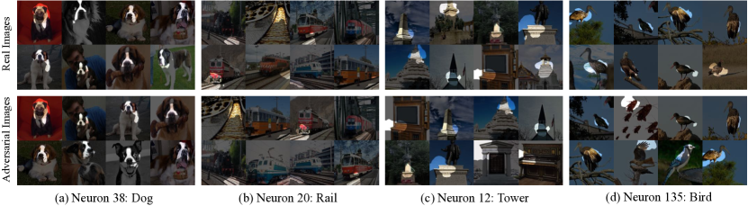
Figure 4: The real and adversarial images with highest activations for neurons in VGG-16-Adv conv5_3 layer.

Experimental Results on ImageNet Dataset

We first show our visualization results. The results are shown in Figure 3 and Figure 4 for neurons in VGG-16 and VGG-16-Adv, respectively. We find that, after adversarial training, the visual concepts are quite similar in both of the real images and adversarial images.This result shows that the network trained with a consistent loss is more interpretable than the normally trained network.

Then we show our quantitave results. We show the average of $consis(n)$ and $consis_{adv}(n)$ of neurons in the last convolutional layer. As shown in Table 1, the consistency level of neurons on the whole image space don’t change much after adversarial training, while the consistency level constrained on the adversarial image subset increases. We also plot the distribution of $consis(n)$ and $consis_{adv}(n)$ of neurons in the last convolutional layer of ResNet-18 and ResNet-18-Adv. As shown in  Figure 5, when showing adversarial samples, the distribution shift left sharply for ResNet-18, while ResNet-18-Adv doesn’t change much.

Table 1: The average of $consis(n)$ and $consis_{adv}(n)$ of neurons in the last convolutional layer in each network. The $consis(n)$ is calculated on the whole image space and the $consis_{adv}(n)$ is calculated on the adversarial image subset.

	$consis(n)$	$consis_{adv}(n)$
AlexNet	0.0162	0.0116
AlexNet-Adv	0.0161	0.0121
VGG-16	0.0296	0.0187
VGG-16-Adv	0.0287	0.0220
ResNet-18	0.0261	0.0133
ResNet-18-Adv	0.0251	0.0206

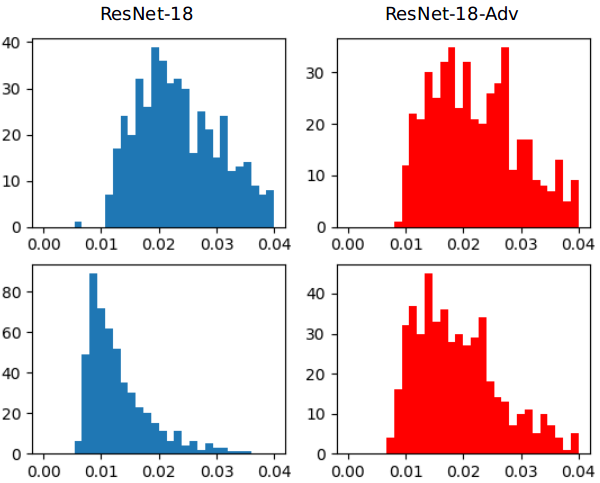
Figure 5: The distribution of $consis(n)$ and $consis_{adv}(n)$ of neurons in the last convolutional layer of ResNet-18 and ResNet-18-Adv. The left two histograms corresponds to ResNet-18 and the right two histograms corresponds to ResNet-18-Adv. The top two histograms corresponds to $consis(n)$ and the bottom two histograms corresponds to $consis_{adv}(n)$.

Experimental Results on Broden Dataset

Table 2: The ratio (%) of neurons that align with semantic concepts for each model, when showing real and adversarial images respectively. There are six types of concepts: colors (C.), textures (T.), materials (M.), scenes (S.), parts (P.) and objects (O.).

	Real Images
	C.	T.	M.	S.	P.	O.
AlexNet	0.4	13.3	0.8	0.4	6.6	17.2
AlexNet-Adv	0.4	20.7	0.0	0.4	4.3	16.4
VGG-16	0.2	11.9	0.8	4.7	10.2	34.6
VGG-16-Adv	0.2	18.0	1.2	5.7	8.6	30.9
ResNet-18	0.0	12.7	0.8	5.9	4.3	33.8
ResNet-18-Adv	0.2	21.3	1.6	6.1	6.8	33.8

	Adversarial Images
	C.	T.	M.	S.	P.	O.
AlexNet	0.4	12.1	0.4	0.0	5.5	10.2
AlexNet-Adv	0.4	18.8	0.0	0.4	4.3	11.3
VGG-16	0.2	2.9	0.0	0.2	3.3	6.4
VGG-16-Adv	0.4	14.1	0.6	1.4	6.4	17.4
ResNet-18	0.0	4.3	0.2	0.6	1.0	6.1
ResNet-18-Adv	0.2	15.0	0.4	1.2	3.1	6.8

For the Broden dataset, we calculate the number of neurons that align with visual concepts for each model. For each model, we also generate a set of adversarial images to evaluate the interpretability of neurons. We show the results in Table 2. It can be seen that for normally trained models, the number of neurons that align with both high-level and low-level semantic concepts decreases significantly by showing adversarial images. On the other hand, the neurons in adversarially trained models are more consistent, in the presence of adversarial images.

Model Performance

Table 3: Accuracy (%) on the ImageNet validation set and adversarial examples generated by FGSM with $\epsilon=1$.

		AlexNet	VGG16	ResNet18
Real	Top-1	54.58	68.15	66.30
	Top-5	78.17	88.30	87.09
Adv.	Top-1	4.44	8.60	4.41
	Top-5	22.94	36.94	31.8
		AlexNet-Adv	VGG16-Adv	ResNet18-Adv
Real	Top-1	43.92	62.55	54.01
	Top-5	68.80	84.66	77.84
Adv.	Top-1	17.45	25.62	27.56
	Top-5	38.12	56.17	55.61

We report the performance of these models on the ImageNet validation set as well as the adversarial examples generated by FGSM in Table 3. We notice that after adversarial training, the accuracy of the models drops about $10\%$. But the models after adversarial training can improve the accuracy against attacks.

References

- [Bau et al. 2017] Bau, D.; Zhou, B.; Khosla, A.; Oliva, A.; and Torralba, A. 2017. Network dissection: Quantifying interpretability of deep visual representations. In CVPR.
- [Doshi-Velez 2017] Doshi-Velez, Finale; Kim, B. 2017. Towards a rigorous science of interpretable machine learning. In eprint arXiv:1702.08608.
- [He et al. 2016] He, K.; Zhang, X.; Ren, S.; and Sun, J. 2016. Deep residual learning for image recognition. In CVPR.
- [Krizhevsky, Sutskever, and Hinton 2012] Krizhevsky, A.; Sutskever, I.; and Hinton, G. E. 2012. Imagenet classification with deep convolutional neural networks. In NIPS.
- [Miller et al. 1990] Miller, G. A.; Beckwith, R.; Fellbaum, C.; Gross, D.; and Miller, K. J. 1990. Introduction to wordnet: An on-line lexical database. International journal of lexicography 3(4):235–244.
- [Russakovsky et al. 2015] Russakovsky, O.; Deng, J.; Su, H.; Krause, J.; Satheesh, S.; Ma, S.; Huang, Z.; Karpathy, A.; Khosla, A.; Bernstein, M.; et al. 2015. Imagenet large scale visual recognition challenge. International Journal of Computer Vision 115(3):211–252.
- [Simonyan and Zisserman 2015] Simonyan, K., and Zisserman, A. 2015. Very deep convolutional networks for large-scale image recognition. In ICLR.
- [Zeiler and Fergus 2014] Zeiler, M. D., and Fergus, R. 2014. Visualizing and understanding convolutional networks. In ECCV.
- [Zhou et al. 2015] Zhou, B.; Khosla, A.; Lapedriza, A.; Oliva, A.; and Torralba, A. 2015. Object detectors emerge in deep scene cnns. In ICLR.