False spin zeros in the angular dependence of magnetic quantum oscillation in quasi-two-dimensional metals

Abstract

The interplay between angular and quantum magnetoresistance oscillations in quasi-two-dimensional metals leads to the angular oscillations of the amplitude of quantum oscillations. This effect becomes pronounced in high magnetic field, when the simple factorization of the angular and quantum oscillations is not valid. The amplitude of quantum magnetoresistance oscillations is reduced at the Yamaji angles, i.e. at the maxima of the angular magnetoresistance oscillations. These angular beats of the amplitude of quantum oscillations resemble and may be confused with the spin-zero effect, coming from the Zeeman splitting. The proposed effect of "false spin zeros" becomes stronger in the presence of incoherent channels of interlayer electron transport and can be used to separate the different contributions to the Dingle temperature and to check for violations from the standard factorization of angular and quantum magnetoresistance oscillations.

I Introduction

Layered quasi-two-dimensional (Q2D) compounds are of great interest to modern condensed matter physics and comprise almost all high-temperatures superconductors, organic metals, intercalated graphites, GaAs layered heterostructures, rare-earth tellurides and numerous other natural and artificial layered conductors. The magnetic quantum oscillations (MQO) and angular dependence of magnetoresistance (MR) are two traditional and common tools to probe the electronic structure of metals.Shoenberg ; Abrik ; Ziman In Q2D metals even the classical MR shows oscillating behavior as a function of tilt angle $\theta$ of magnetic field with respect to the normal to conducting layers,KartsAMRO1988 ; Yam called the angular magnetoresistance oscillations (AMRO). Now, together with MQO, AMRO are extensively used to study the electronic structure in layered organic metals (see, e.g., MarkReview2004 ; Singleton2000Review ; KartPeschReview ; OMRev ; MQORev ; Brooks2006 ; LebedBook for reviews), in heterostructures,Kuraguchi2003 ruthenates,Bergemann2003 tungsten bronze,AMROBronze and even in cuprate high-temperature superconductors.HusseyNature2003 ; AbdelNature2006 ; AbdelPRL2007AMRO ; McKenzie2007 ; AMROKartsovnikNd ; AMROCuprate2015Analytis

The Fermi surface in Q2D metals has the shape of a warped cylinder, which corresponds to the strongly anisotropic electron dispersion

$$\epsilon_{3D}\left(\mathbf{k}\right)\approx\epsilon_{2D}\left(k_{x},\,k_{y}\right)-2t_{z}\cos(k_{z}d),$$ (1)

where $\hbar\left\{k_{x},\,k_{y},\,k_{z}\right\}$ are the electron momentum components, $\hbar$ is the Planck’s constant, $d$ is the interlayer distance, and the interlayer transfer integral $t_{z}$ is much less than the Fermi energy $E_{F}$. In some cases, especially in low-symmetry crystals, $t_{z}=t_{z}\left(k_{x},\,k_{y}\right)$ depends on in-plane momentum, which affects AMRO and MQO.Mark92 ; Singleton2001 ; Bergemann ; GrigAMRO2010 However, to describe most compounds it is sufficient to take $t_{z}\left(k_{x},\,k_{y}\right)\approx const$. The geometrical explanation of AMROYam for the electron dispersion in Eq. (1) is based on the observation that for the quadratic and isotropic in-plane electron dispersion $\epsilon_{2D}\left(k_{x},k_{y}\right)=\hbar^{2}\left(k_{x}^{2}+k_{y}^{2}\right)/2m^{\ast}$ and for $t_{z}\approx const$ the cross-section areas of such warped-cylindrical Fermi surface in the first order in $t_{z}$ become independent on $k_{z}$ for some tilt angles $\theta=\theta_{Yam}$ of magnetic field, now called the Yamaji angles.MarkReview2004 ; Singleton2000Review ; KartPeschReview ; OMRev ; MQORev ; Brooks2006 ; LebedBook The Yamaji angles give the minima of the angular dependence of interlayer conductivity $\sigma_{zz}\left(\theta\right)$ and correspond to the zeros of the Bessel function $J_{0}\left(\kappa\right)$, where $\kappa\equiv k_{F}d\tan\theta$ and $k_{F}$ is the in-plane Fermi momentum. The direct calculation of interlayer conductivity from the Boltzmann transport equation in the $\tau$-approximation with the electron dispersion in Eq. (1) givesYagi1990

$$\frac{\sigma_{zz}\left(\theta\right)}{\sigma_{zz}}=\left[J_{0}\left(\kappa\right)\right]^{2}+2\sum_{\nu=1}^{\infty}\frac{\left[J_{\nu}\left(\kappa\right)\right]^{2}}{1+\left(\nu\omega_{c}\tau\right)^{2}}\equiv\Phi_{AMRO}\left(\theta\right),$$ (2)

where $\tau$ is the electron mean free time, and the cyclotron frequency $\omega_{c}$ in Q2D metals depends on the tilt angle $\theta$ of magnetic field: $\omega_{c}\equiv eB_{z}/m^{\ast}c=\omega_{c0}\cos\theta$, where $B_{z}$ is the component of magnetic field perpendicular to conducting layers, $e$ is the electron charge, $m^{\ast}$ is the effective electron mass and $c$ is the light velocity. In Ref. Yagi1990 the MQO are neglected and $\sigma_{zz}\approx\sigma_{zz}^{0}$, where the interlayer conductivity without magnetic field

$$\sigma_{zz}^{0}=e^{2}\rho_{F}\left\langle v_{z}^{2}\right\rangle\tau=2e^{2}t_{z}^{2}m^{\ast}\tau d/\pi\hbar^{4},$$ (3)

$\rho_{F}=m^{\ast}/\pi\hbar^{2}d$ is the 3D density of states (DoS) at the Fermi level in the absence of magnetic field per two spin components, and the mean squared interlayer electron velocity along interlayer direction is $\left\langle v_{z}^{2}\right\rangle=2t_{z}^{2}d^{2}/\hbar^{2}$. Eq. (2) agrees with the result of Yamaji at $\omega_{c}\tau\rightarrow\infty$. A microscopic calculation of Q2D AMRO using the Kubo formula and electron dispersion in Eq. (1), neglecting the MQO, also gives Eq. (2) when the number of filled Landau levels (LLs) $n_{LL}^{F}\gg 1$.Kur Assumption $\sigma_{zz}\approx\sigma_{zz}^{0}$ in Eq. (2) is valid only in weak magnetic field, such that $\omega_{c}\tau\ll 1$, so that MQO are negligible and AMRO are also weak. In strong magnetic field, $\omega_{c}\tau\gtrsim 1$, when both AMRO and MQO are strong, Eq. (2) is, generally, incorrect.

The standard theory of MQO and of AMRO considers these two phenomena independently, i.e. neglecting their interplay, which is valid only in the limit of weak MQO and AMRO.Abrik ; Ziman Usually, to analyze the experimental data in quasi-2D metals in the high-field limit one applies Eq. (2) with a phenomenological replacement $\sigma_{zz}=\sigma_{zz}^{MQO}\left(B_{z}\right)$, where $\sigma_{zz}^{MQO}\left(B_{z}\right)$ depends on magnetic field $\boldsymbol{B}$ only due to the MQO. Then the angular and field dependence of $\sigma_{zz}\left(\boldsymbol{B}\right)$ factorize:

$$\sigma_{zz}\left(\boldsymbol{B}\right)=\Phi_{AMRO}\left(\theta\right)\cdot\sigma_{zz}^{MQO}\left(B\right),$$ (4)

where $\Phi_{AMRO}\left(\theta\right)$ is given by Eq. (2) and depends on the field strength $B$ via the product $\omega_{c}\tau$, and $\sigma_{zz}=\sigma_{zz}^{MQO}\left(B\right)=\sigma_{zz}^{0}+\tilde{\sigma}_{zz}\left(B\right)$ include MQO. The oscillating part $\tilde{\sigma}_{zz}$ of conductivity is given by a sum of MQO with all frequencies $F^{a}=S_{ext}^{a}\hbar c/2\pi e$, determined by the FS extremal cross-section areas $S_{ext}^{a}$:Shoenberg ; Abrik ; CommentSO ; GKM

$$\frac{\sigma_{zz}}{\sigma_{zz}^{0}}\approx\sum_{a}\frac{g_{0,a}}{g_{tot}}\left[1+2\sum_{k=1}^{\infty}A_{a}\left(k\right)\cos\left(2\pi k\frac{F^{a}}{B}-\phi_{a}\right)\right],$$ (5)

where the total density of states (DoS) at the Fermi level $g_{tot}=\sum_{a}g_{0,a}$ is a sum of the contributions $g_{0,a}$ from all FS pockets $a$, and the phase shift $\phi_{a}\approx\pi/4$. The MQO amplitudes $A_{a}\left(k\right)$ depend on the FS geometry, being also proportional to the product of three damping factors:Shoenberg ; Abrik ; Ziman the Dingle factor

$$R_{D}\left(k\right)=\exp\left(\frac{-\pi k}{\omega_{c}\tau}\right),$$ (6)

the temperature damping factor

$$R_{T}(k)=\frac{2\pi^{2}k_{B}Tk/\hbar\omega_{c}}{\sinh\left(2\pi^{2}k_{B}Tk/\hbar\omega_{c}\right)},$$ (7)

and the spin factor $R_{S}$, in Q2D metals given byShoenberg ; Abrik ; Ziman

$$R_{S}\left(k\right)=\cos\left(\frac{\pi k\Delta_{Z}}{\hbar\omega_{c}}\right)=\cos\left(\frac{\pi gkm^{\ast}}{2m_{e}\cos\theta}\right),$$ (8)

where the Zeeman splitting $\Delta_{Z}=g\hbar eB/2m_{e}c=gB\mu_{B}$ of electron energy is independent of $\theta$ if the electron $g$-factor $g$ does not depend on $\theta$.Commentgfactor In Q2D metals $\hbar\omega_{c}\propto\cos\theta$, and the spin factor $R_{S}$ results to strong oscillating angular dependence of the MQO amplitude, given by Eq. (8), which is typical to 2D and Q2D metals and allows measuring the electron $g$-factor from the so-called spin zeros – the tilt angles $\theta_{s}$, where the factor in Eq. (8) becomes zero.

In Q2D metals with electron dispersion in Eq. (1) each FS pocket is a warped cylinder, giving two FS extremal cross-sections. At $t_{z}\gg\hbar\omega_{c}$ the difference of these two extremal FS cross-sections areas is much larger than the LL separation, and one can use the 3D formula in Eq. (5), derived in the lowest order in $\hbar\omega_{c}/t_{z}$. The simplest (but approximate at $\hbar\omega_{c}\sim t_{z}$) generalization of Eq. (5) for $\hbar\omega_{c}\lesssim t_{z}$, by analogy to the quasi-2D DoS,Champel2001 is

$$\frac{\sigma_{zz}}{\sigma_{zz}^{0}}\approx\sum_{a}\frac{g_{0,a}}{g_{tot}}\left[1+2\sum_{k=1}^{\infty}A_{a}\left(k\right)\cos\left(\frac{2\pi kF^{a}}{B}\right)\right],$$ (9)

where the amplitudes

$$A_{\alpha}\left(k\right)=\left(-1\right)^{k}J_{0}\left(\frac{4\pi kt_{z}}{\hbar\omega_{c}}\right)R_{D}\left(k\right)R_{T}\left(k\right)R_{S}\left(k\right),$$ (10)

and the summation over $\alpha$ in Eq. (9) is the summation over cylindrical FS pockets rather than over FS extremal cross sections $a$ as in Eq. (5). Note that, contrary to Eq. (5), in Eq. (9) the phases $\phi_{a}$ are absent; in fact these phases are contained in the Bessel’s functions $J_{0}\left(4\pi kt_{z}/\hbar\omega_{c}\right)$ in the amplitudes $A_{\alpha}\left(k\right)$. At $\hbar\omega_{c}\sim t_{z}$ the higher-order terms in $\hbar\omega_{c}/t_{z}$ become important, and Eqs. (9) and (10) modifyPhSh ; SO ; Shub ; ChampelMineev (see, e.g., Eqs. (18)-(21) of Ref. Shub or Eqs. (13)-(15) of Ref. ChampelMineev ), producing two new physical effect: the phase shift of beatsPhSh ; Shub and the slow oscillations of magnetoresistance.SO ; Shub

When MQO and AMRO are strong, their interplay may become essential. Then not only Eqs. (2) but also Eq. (4) may be incorrect, i.e. the conductivity is not simply a product of the AMRO factor in Eq. (2) and the MQO factor in Eq. (5) or (9). Recently, the influence of strong MQO on the AMRO factor in Eq. (2) was studied.TarasPRB2014 It was found that in the high-field limit $\omega_{c}\gg 1/\tau,\,t_{z}/\hbar$ the strong MQO modify AMRO factor in Eq. (2), keeping the AMRO period almost untouched but changing the AMRO amplitude and its magnetic-field dependence.TarasPRB2014 Also the shape of Landau levels (LL), which is not Lorentzian at $\omega_{c}\gg 1/\tau,\,t_{z}/\hbar$, is reflected in the AMRO damping. For example, for Gaussian LL shape the terms with $\nu\neq 0$ are stronger damped than in Eq. (2) and given by Eq. (33) of Ref. TarasPRB2014 , which increases the AMRO amplitude. Thus, the interplay between MQO and AMRO may be considerable at $\omega_{c}\tau\gg 1$.

In the present paper we study the influence of AMRO on MQO, especially on the angular dependence of the amplitude of MQO of magnetoresistance. We show that this influence is rather strong, and in high magnetic field, at $\omega_{c}\gg 1/\tau,\,t_{z}/\hbar$, may lead to a new qualitative phenomenon – the false spin zeros of MQO of MR.

II The model and general formulas

II.1 Two-layer model

To study the influence of AMRO on MQO, we consider strongly anisotropic Q2D metals in a high magnetic field, when $\omega_{c}\gg 1/\tau,\,t_{z}/\hbar$ and both AMRO and MQO are strong. In this limit, to calculate the interlayer conductivity $\sigma_{zz}$ one can apply the two-layer model,MosesMcKenzie1999 ; WIPRB2011 ; TarasPRB2014 where $\sigma_{zz}$ is calculated as a tunnelling conductivity between two adjacent conducting layers using Kubo formula with electron Green’s function taken inside 2D conducting layer with disorder (see Appendix A). It was shown that this two-layer model is equivalent to the 3D models with strongly anisotropic electron dispersion $\epsilon_{3D}\left(\mathbf{k}\right)$ if $\omega_{c}\gg 1/\tau,\,t_{z}/\hbar$.GrigPRB2013 Then

$$\sigma_{zz}\left(T\right)=\frac{1}{2}\sum_{s=\pm 1}\int d\varepsilon\left[-n_{F}^{\prime}(\varepsilon)\right]\sigma_{zz}\left(\varepsilon+s\Delta_{Z}\right),$$ (11)

where $n_{F}^{\prime}(\varepsilon)=-1/\{4T\cosh^{2}\left[(\varepsilon-\mu)/2T\right]\}$ is the derivative of the Fermi distribution function, $\mu=E_{F}$ is the chemical potential of electrons, andTarasPRB2014

$$\frac{\sigma_{zz}\left(\varepsilon\right)}{\sigma_{zz}^{0}} = \frac{2\Gamma_{0}\hbar\omega_{c}}{\pi}\sum_{n,p\in Z}Z(n,p)\times$$ (12)

$$\times\text{Im}G(\varepsilon,\,n)\text{Im}G(\varepsilon,\,n+p).$$

Here the function $Z$ comes from the overlap of electron wave functions on adjacent layers, producing AMRO, and is given by Eq. (12) of Ref. TarasPRB2014 , which coincides with the square of Eq. (9) in Ref. Raikh . The interlayer conductivity in the absence of magnetic field is given by $\sigma_{zz}^{0}=2e^{2}\tau_{0}m^{\ast}t_{z}^{2}d/\pi\hbar^{4}$, and $\Gamma_{0}=\hbar/2\tau_{0}$. Eq. (12) is valid for arbitrary electron Green’s functions

$$G(\varepsilon,\,n)=\frac{1}{\varepsilon-\hbar\omega_{c}(n+1/2)-\Sigma(\varepsilon)},$$ (13)

which contain the self-energy part $\Sigma(\varepsilon)$ determined by disorder. Below we neglect the electron-electron (e-e) interaction, which can be used only when many LL are filled, $n_{LL}^{F}=\left\lceil\mu/\hbar\omega_{c}\right\rceil\gg 1$, and the e-e interaction is effectively screened.KukushkinUFN1988 ; Aleiner1995 In this limit $n_{LL}^{F}\gg 1$ the function $Z(n,p)$ simlifiesTarasPRB2014 ; Kur

$$Z(n,p)\approx Z(n_{LL}^{F},p)\approx J_{p}^{2}\left(k_{F}d\tan\theta\right)\equiv J_{p}^{2}\left(\kappa\right).$$ (14)

With notations $\Gamma(\varepsilon)=\left|\text{{Im}}\Sigma\left(\varepsilon\right)\right|=-$Im$\Sigma^{R}\left(\varepsilon\right)$ and $\varepsilon^{\ast}\equiv\varepsilon-$Re$\Sigma(\varepsilon)$, the imaginary part of the electron Green’s function is

$$\text{Im}G(\varepsilon,\,n)=-\Gamma(\varepsilon)/\left[(\varepsilon^{\ast}-\hbar\omega_{c}(n+1/2))^{2}+\Gamma^{2}(\varepsilon)\right],$$ (15)

Using also the notations $\varepsilon^{\ast}\equiv\varepsilon-$Re$\Sigma(\varepsilon)$, $\gamma_{0}=2\pi\Gamma_{0}/\hbar\omega_{c}$, $\gamma\equiv 2\pi\left|\text{Im}\Sigma(\varepsilon)\right|/\hbar\omega_{c}$, and $\alpha\equiv 2\pi\varepsilon^{\ast}/\hbar\omega_{c}$, from Eqs. (12)-(15) one obtains

$$\frac{\sigma_{zz}(\varepsilon)}{\sigma_{zz}^{0}}=\frac{\Gamma_{0}}{\Gamma(\varepsilon)}\sum_{p=-\infty}^{\infty}S_{p}\left[J_{p}\left(\kappa\right)\right]^{2},$$ (16)

where

$$S_{0} \equiv \sum_{n\in Z}\frac{(2/\pi)\hbar\omega_{c}\Gamma^{3}}{\left[\left(\varepsilon^{\ast}-\hbar\omega_{c}\left(n+\frac{1}{2}\right)\right)^{2}+\Gamma^{2}\right]^{2}}=$$

$$= \frac{\sinh(\gamma)}{\cos(\alpha)+\cosh(\gamma)}-\gamma\frac{1+\cos(\alpha)\cosh(\gamma)}{(\cos(\alpha)+\cosh(\gamma))^{2}}$$

in agreement with Eq. (23) of Ref. ChampelMineev , and for $p\neq 0$

$$S_{p}\equiv\sum_{n\in Z}\frac{\left(2/\pi\right)\hbar\omega_{c}\Gamma^{3}}{\left[\left(\varepsilon^{\ast}-\hbar\omega_{c}\left(n+1/2\right)\right)^{2}+\Gamma^{2}\right]}\times$$

$$\times\frac{1}{\left[\left(\varepsilon^{\ast}-\hbar\omega_{c}\left(n+p+1/2\right)\right)^{2}+\Gamma^{2}\right]}=$$

$$=\frac{\sinh(\gamma)}{\left(\cos(\alpha)+\cosh(\gamma)\right)\left[1+(p\pi/\gamma)^{2}\right]}.$$ (18)

Equations (16)-(18) give both AMRO and MQO for arbitrary (unknown yet) electron self-energy $\Sigma\left(\varepsilon\right)$.

At $\gamma\gg 1$ (weak field limit) the second term is Eq. (II.1) is exponentially small, so that $S_{0}$ in Eq. (II.1) is the same as $S_{p}$ in Eq. (18) at $p=0$. Hence, as expected, at $\gamma\gg 1$ we confirm Eqs. (2) and (4). However, at $\gamma\ll 1$ (high-field limit) the second term in Eq. (II.1) is important, and the function $S_{0}$ in Eq. (II.1) becomes completely different from $S_{p}(p=0)$ in Eq. (18). This means that at $\gamma\ll 1$ Eqs. (2) and (4) are not valid for any self-energy part $\Sigma\left(\varepsilon\right)$. The difference between the functions $S_{0}$ and $S_{p}(p=0)$, leadinig to the violation of Eqs. (2) and (4), is illustrated in Fig. 1 at $\left|\text{{Im}}\Sigma\left(\varepsilon\right)\right|=\Gamma_{0}=const$ and is clearly seen already from the expansions of $S_{0}$ and of $S_{p}(p=0)$ at $\gamma\rightarrow 0$:

$$S_{0}\left(\gamma\rightarrow 0\right)=\frac{2-\cos(\alpha)}{[1+\cos(\alpha)]^{2}}\frac{\gamma^{3}}{3}+O[\gamma]^{5},$$ (19)

$$S_{p}\left|{}_{\begin{subarray}{c}\gamma\rightarrow 0,\\ p=0\end{subarray}}\right.=\frac{\gamma}{1+\cos(\alpha)}-\frac{2-\cos(\alpha)}{[1+\cos(\alpha)]^{2}}\frac{\gamma^{3}}{6}+O[\gamma]^{5}.$$

For example, in the minima of MQO of conductivity, i.e. at $\alpha=0$, Eq. (19) shows that the function $S_{0}$ is much smaller than $S_{p}(p=0)$ at $\gamma\rightarrow 0$:

$$S_{0}\left|{}_{\begin{subarray}{c}\gamma\rightarrow 0,\\ \alpha=0\end{subarray}}\right.\approx\frac{\gamma^{3}}{12}\ll S_{p}\left|{}_{\begin{subarray}{c}\gamma\rightarrow 0,\\ p=0\\ \alpha=0\end{subarray}}\right.\approx\frac{\gamma}{2}.$$ (20)

These expansions (19) and (20) are valid at any $\alpha$ except the proximity of the point $\alpha=\pi$, where the denominator in (19) vanishes. At $\alpha=\pi$ and $\gamma\rightarrow 0$ the expansion of Eqs. (II.1) and (18) gives

$$S_{0}\left|{}_{\begin{subarray}{c}\gamma\rightarrow 0,\\ \alpha=\pi\end{subarray}}\right.\approx\frac{4}{\gamma},~{}~{}S_{p}\left|{}_{\begin{subarray}{c}\gamma\rightarrow 0,\\ p=0\\ \alpha=\pi\end{subarray}}\right.\approx\frac{2}{\gamma},$$ (21)

i.e. in the maxima of MQO at $\gamma\rightarrow 0$ the function $S_{0}$ is only twice larger than $S_{p}(p=0)$.

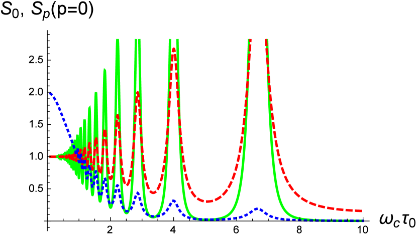
Figure 1: (Color on-line) The comparison of the functions $S_{0}\left(B_{z}\right)$ (solid green line) and $S_{p}\left(B_{z}\right)$ at $p=0$ (dashed red line), given by Eqs. (II.1) and (18) at $\left|\text{{Im}}\Sigma\left(\varepsilon\right)\right|=\Gamma_{0}=const$ and $\alpha=20\gamma$. Both functions show oscillations around the same background, but the amplitude of the oscillations of $S_{0}\left(B_{z}\right)$ are much stronger at $\gamma\ll 1$. The dotted blue line gives $2S_{p}\left(p=1\right)$ for comparison.

As was shown in Refs. Shub ; ChampelMineev , the function $S_{0}$ differs from $S_{p}(p=0)$ because of the extra term $G_{R}^{2}$ in the Kubo formula for conductivity. This term contributes only a second-order poles in the integrand over $\varepsilon$, which does not affect the result at zero magnetic field but contributes the term $\sim$ $\gamma$ to the amplitudes of MQO harmonics of conductivity.Shub ; ChampelMineev

II.2 Electron Green’s function and self energy

The expression (13) for the electron Green’s function contains the self-energy $\Sigma\left(\varepsilon\right)$, which at low temperature mainly comes from the scattering on impurity potential

$$V_{i}\left(\mathbf{r}\right)=\sum_{j}U\delta^{3}\left(\mathbf{r}-\mathbf{r}_{j}\right).$$ (22)

The impurities are assumed to be short-range (point-like) and randomly distributed with volume concentration $n_{i}$. The scattering by this impurity potential is spin-independent. In the non-crossing (self-consistent single-site) approximation the electron self-energy satisfies the following equation:Ando

$$\Sigma(\varepsilon)=\frac{n_{i}U}{1-UG\left(\varepsilon\right)},$$ (23)

where the averaged Green’s function in the coinciding pointsChampelMineev ; Grigbro

$$G\left(\varepsilon\right)=\sum_{n,k_{y},k_{z}}G\left(\varepsilon,n\right)=\frac{g_{LL}}{d}\sum_{n=0}^{+\infty}G\left(\varepsilon,n\right)$$ (24)

$$\approx\frac{g_{LL}}{d}\sum_{n=-\infty}^{+\infty}\frac{1}{\varepsilon-\hbar\omega_{c}(n+1/2)-\Sigma(\varepsilon)}$$ (25)

$$=-\frac{\pi g_{LL}}{\hbar\omega_{c}d}\tan\left[\pi\frac{\varepsilon-\Sigma(\varepsilon)}{\hbar\omega_{c}}\right].$$ (26)

The summation over $k_{y}$ in Eq. (24) gives the LL degeneracy $g_{LL}=eB_{z}/2\pi\hbar c$, and the summation over $k_{z}$ gives $1/d$. Strictly speaking, in Eqs. (24) the summation over $n$ must be cut at $n_{\max}\sim W/\hbar\omega_{c}$, where $W\sim\mu$ is the band width, as the expression logarithmically diverges. Similarly, in Eq. (25) we extended the summation over $n$ from $-\infty$, because the neglected difference $\sum_{n=-\infty}^{0}G\left(\varepsilon,n\right)\approx\ln\left(W/\mu\right)/\hbar\omega_{c}=const$ does not affect observable quantities. In the self-consistent Born approximation (SCBA), used below, the neglected difference is equivalent to the constant shift of chemical potential.

It is convenient to use the normalized electron Green’s function

$$g\left(\varepsilon\right)\equiv G\left(\varepsilon\right)\hbar\omega_{c}d/\pi g_{LL}.$$ (27)

To obtain the monotonic growth of longitudinal interlayer magnetoresistanceWIPRB2011 ; GrigPRB2013 ; WIJETP2011 and other qualitative physical effectsTarasPRB2014 , the SCBA is sufficient, which instead of Eq. (23) gives

$$\Sigma(\varepsilon)-n_{i}U=n_{i}U^{2}G\left(\varepsilon\right)=\Gamma_{0}g\left(\varepsilon\right).$$ (28)

Here we used that the zero-field level broadening is $\Gamma_{0}=\pi n_{i}U^{2}\nu_{3D}=\pi n_{i}U^{2}g_{LL}/(d\hbar\omega_{c})=\hbar/2\tau_{0}$. Below we also neglect the constant energy shift $n_{i}U$ in Eq. (28), which does not affect physical quantities as conductivity.

Eqs. (26)-(28) give the equations on the Green’s function $g\equiv g\left(\varepsilon\right)$:

$$\text{Im}g=\frac{\sinh\left(\gamma_{0}\text{Im}g\right)}{\cosh\left(\gamma_{0}\text{Im}g\right)+\cos\left(\alpha\right)}=\frac{\gamma}{\gamma_{0}},$$ (29)

$$\text{Re}g=\frac{-\sin\left(\alpha\right)}{\cosh\left(\gamma_{0}\text{Im}g\right)+\cos\left(\alpha\right)},$$ (30)

or the equations for the electron self-energy $\Sigma^{R}(\varepsilon)$:

$$\frac{\gamma}{\gamma_{0}}=\frac{\sinh\left(\gamma\right)}{\cosh\left(\gamma\right)+\cos\left(\alpha\right)},$$ (31)

$$\delta\equiv\alpha-\frac{2\pi\varepsilon}{\hbar\omega_{c}}=\frac{\gamma_{0}\sin\left(\alpha\right)}{\cosh\left(\gamma\right)+\cos\left(\alpha\right)}.$$ (32)

Here we have used the notations introduced after Eq. (15). The solution of Eq. (31) gives Im$\Sigma(\alpha)$, while Eq. (32) allows to find $\alpha\left(\varepsilon\right)$ and Re$\Sigma(\varepsilon)$. The system of Eqs. (31) and (32) differs from Eq. (30) of Ref. ChampelMineev even in the absence of electron reservoir (at $R=0$), because in Eq. (30) of Ref. ChampelMineev the oscillating real part of the electron self energy is neglected, which leads to a different dependence of $\sigma_{zz}(B_{z})$.GrigPRB2013

Eq. (31) allows to find the value $\gamma_{0c}$, when the LLs become isolated in SCBA, i.e. when the DoS and Im$\Sigma^{R}(\varepsilon)$ between LLs become zero. In the middle between two adjacent LLs $\cos\left(\alpha\right)=1$, and equation (31) for $\gamma_{min}$ at conductivity minima becomes:

$$\frac{\gamma_{min}}{\gamma_{0}}=\frac{\sinh\left(\gamma_{min}\right)}{\cosh\left(\gamma_{min}\right)+1}=\tanh\left(\gamma_{min}/2\right).$$ (33)

This equation always has a trivial solution $\gamma=0$. However, at $\gamma_{0}>\gamma_{0c}=2$, corresponding to $\pi\Gamma_{0}>\hbar\omega_{c}$, Eq. (33) also has a non-zero solution. This nonzero solution means a finite DoS at energy between LLs, i.e. at $\pi\Gamma_{0}<\hbar\omega_{c}$ in SCBA the LLs become isolated, which affects physical observables, e.g. leads to a monotonic growth of $\sigma_{zz}(B_{z})$.Grigbro

In middle of LL $\cos\left(\alpha\right)=-1$, and equation (31) for $\gamma_{max}$ at conductivity maxima becomes:

$$\frac{\gamma_{max}}{\gamma_{0}}=\frac{\sinh\left(\gamma_{max}\right)}{\cosh\left(\gamma_{max}\right)-1}=\coth\left(\gamma_{max}/2\right).$$ (34)

This equation always has a non-zero solution.

Any additional Fermi-surface parts, which are not responsible for the given MQO, create an extra density of states (DoS) at the Fermi level. This additional DoS does not oscillate with the same frequency and acts as an electron reservoir,ChampelMineev ; GrigChemPotOsc ; ChampelChemPotOsc smearing the MQO. This additional DoS does not oscillate at all if it comes from open Fermi-surface parts. In this case Eq. (31) modifies to

$$\frac{\gamma}{\gamma_{0}}=\left(\frac{\sinh\left(\gamma\right)}{\cosh\left(\gamma\right)+\cos\left(\alpha\right)}+R\right)/\left(1+R\right),$$ (35)

similar to Eq. (24) of Ref. ChampelMineev , where $R$ is the ratio of the reservoir DoS to the average DoS on the Fermi-surface pocket responsible for MQO.

III Interplay between angular and quantum magnetic oscillations

The influence of MQO on AMRO was already studied recently.TarasPRB2014 In this section we analyze the influence of AMRO on MQO of interlayer conductivity using the formulas in the previous section II. As it was shown in Sec. IIA, the violation of Eqs. (2) and (4) and new interesting effects appear only in the high-field limit $\gamma\ll 1$ and only because of the difference between the functions $S_{0}$ and $S_{p}\left(p=0\right)$ given by Eqs. (II.1) and (18). In this section we consider two limiting cases: (i) the limit of large electron reservoir, when $\gamma\approx const$, and (ii) the limit of zero electron reservoir, when there are no other Fermi-surface pockets except the one responsible for MQO.

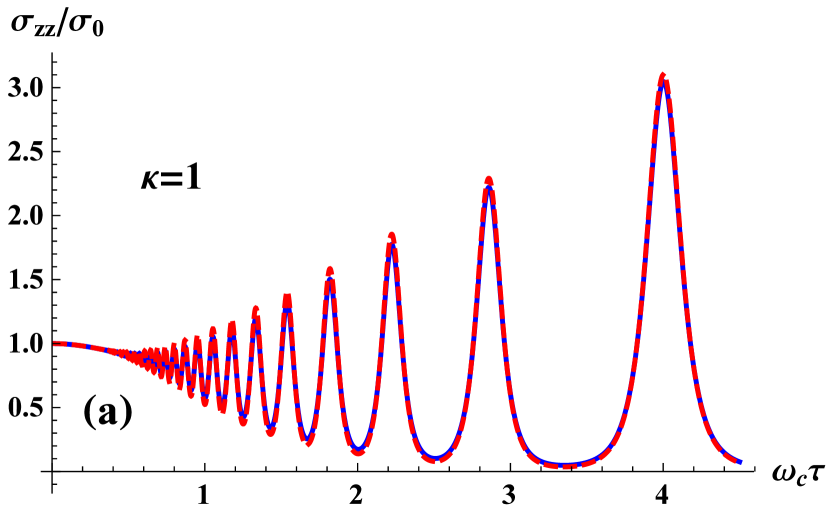
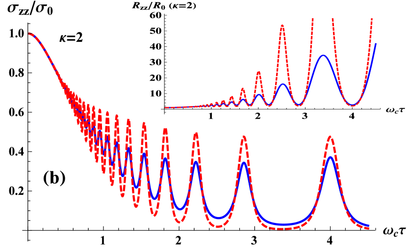
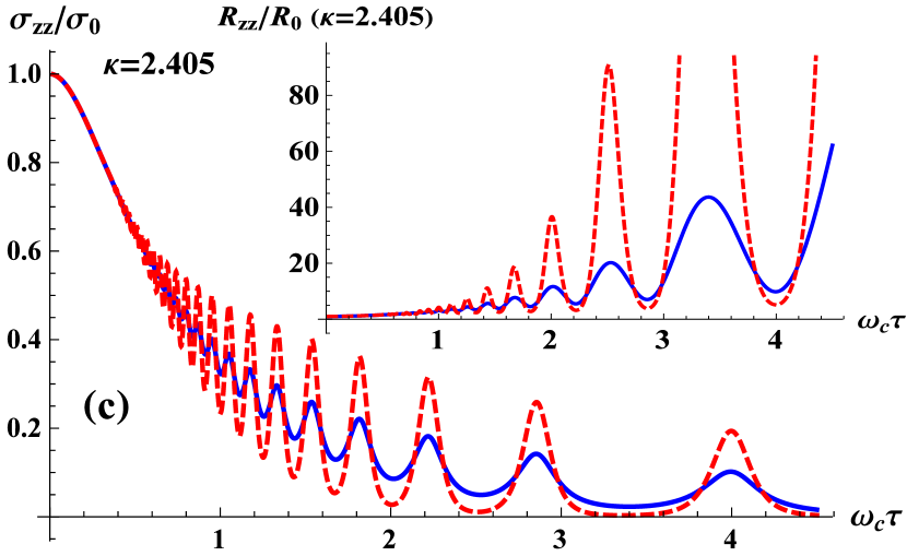
Figure 2: (Color on-line) The comparison of the new formula for conductivity $\sigma_{zz}^{new}(B_{z})$, given by Eqs. (16)-(18) and shown by solid blue line, with $\sigma_{zz}^{old}(B_{z})$, given by Eqs. (4),(2) with $\sigma_{zz}^{MQO}\left(B\right)=\sigma_{zz}^{0}S_{0}\left(B_{z}\right)$ and shown by dashed red line. For this comparison we take three different values of $\kappa\equiv k_{F}d\tan\theta$: $\kappa_{1}=1$, $\kappa_{2}=2$, and $\kappa_{3}=2.405$. The latter corresponds to the first Yamaji angle. The inserts show resistivity $R_{zz}(B_{z})\approx 1/\sigma_{zz}(B_{z})$.

III.1 Limit of large electron reservoir and $\left|\text{{Im}}\Sigma\left(\varepsilon\right)\right|\approx const$

The violation of Eqs. (2) and (4) should be strongest in the minima and maxima of conductivity MQO, where the the functions $S_{0}$ and $S_{p}\left(p=0\right)$ are most different (see Fig. 1). Additionally, the violation of Eqs. (2) and (4) is expected to be most evident near the Yamaji angles, where the term with $p=0$ in Eq. (16) is reduced as compared to the terms with $p\neq 0$.

To check how strong are these deviations from Eqs. (2) and (4) at $\left|\text{{Im}}\Sigma\left(\varepsilon\right)\right|\approx const$, in Fig. 2 we compare $\sigma_{zz}^{new}(\varepsilon)$ calculated using Eqs. (16)-(18) and $\sigma_{zz}^{old}(\varepsilon)$ calculated using Eqs. (4),(2) and Eq. (23) of Ref. ChampelMineev , i.e. $\sigma_{zz}^{MQO}\left(B\right)=\sigma_{zz}^{0}S_{0}$. From this comparison one sees that indeed the notable violation from Eqs. (2) and (4) appears at $\left|\text{{Im}}\Sigma\left(\varepsilon\right)\right|\approx const$ only near the Yamaji angles. These deviations do not change the frequency or the phase of MQO, but considerably reduce their amplitude. This decrease of MQO amplitude near the Yamaji angles as compared to the prediction of Eqs. (2) and (4) is even more clear on the magnetoresistance $R_{zz}\approx 1/\sigma_{zz}$, shown in the inserts to Fig. 2. Our result that in the Yamaji angles the MQO amplitude decreases contradicts the general opinion that the magnetoresistance oscillations should be stronger in the Yamaji angles because the system becomes effectively two-dimensional. Fig. 2 also illustrate a strong influence of AMRO on the amplitude of MQO.

The angular dependence of conductivity and of magnetoresistance as a functions of the tilt angle $\theta$ for a constant magnetic field strength $B_{0}$, calculated using Eqs. (11),(16)-(18), are plotted in Fig. 3 at two temperatures: $T=0.1\Gamma_{0}$ (blue solid line) and at $T=0.4\Gamma_{0}$ (red dashed line). $E_{F}=201\Gamma_{0}$ and $\omega_{c0}\tau_{0}=5$ at $\theta=0$. The fast quantum oscillations come from the angular dependence of normal-to-layer component $B_{z}=B_{0}\cos\theta$ of magnetic field, which enters the MQO. According to the above analytical estimates, the amplitude of MQO considerably decreases near the Yamaji angles, which in Fig. 3 is seen as the angular oscillations of the amplitude of MQO. In the analysis of experimental data on magnetoresistance such beats of the MQO amplitude may be mistakenly interpreted as spin zeros. We suggest the name false spin zeros for this phenomenon of the angular beats of MQO amplitude due to the interplay between AMRO and MQO in quasi-2D metals. Increasing of temperature damps the MQO, but these ”false spin zeros” are still visible.

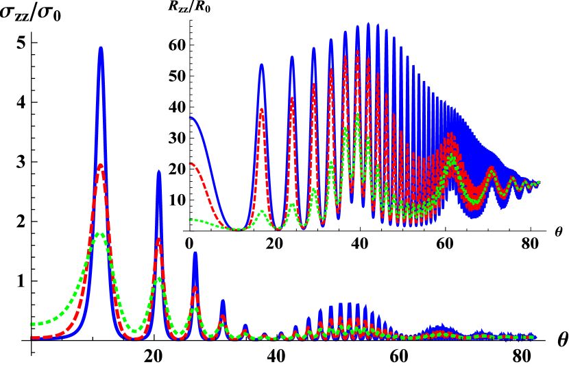
Figure 3: (Color on-line) The angular dependence of conductivity (main figure) and magnetoresistance (insert figure) at $k_{F}d=3$, $\omega_{c0}\tau_{0}=5$ and at three temperatures: $T=0.1\Gamma_{0}$ (blue solid line), $T=0.5\Gamma_{0}$ (red dashed line), and $T=\Gamma_{0}$ (green dotted line). The minima of MQO amplitude, arising from the influence of AMRO on MQO, may be erroneously treated as spin-zeros.

The false spin zeros become even more pronounced if one takes into account the incoherent channels of interlayer conductivity, which come from crystal imperfections, from resonance impurities between the conducting layers,Abrikosov1999 ; Maslov ; Incoh2009 or from polaron tunnellingLundin2003 ; Ho . The incoherent channels produce additional term $\sigma^{i}_{zz}$ for the interlayer conductivity. This term has neither angular nor quantum oscillations and shifts conductivity in Fig. 3 upward by a constant. The total conductivity is a sum of the coherent and incoherent conductivity channels: $\sigma^{tot}_{zz}=\sigma_{zz}^{coh}+\sigma^{i}_{zz}$. Usually, in clean metals the ratio $\sigma^{i}_{zz}/\sigma_{0}\ll 1$. In Fig. 4 we plot the angular dependence of interlayer magnetoresistance $R_{zz}=1/\sigma^{tot}_{zz}$ for two different values of this ratio: $\sigma^{i}_{zz}/\sigma_{0}=0.04$ (Fig. 4a) and $\sigma^{i}_{zz}/\sigma_{0}=0.2$ (Fig. 4b). The magnetic field strength in Fig. 4 corresponds to $\omega_{c0}\tau_{0}=5$ at $\theta=0$, and $k_{F}d=3$. The false spin zeros, seen as the angular beats of MQO amplitude, in Fig. 4 are clearer than in Fig. 3.

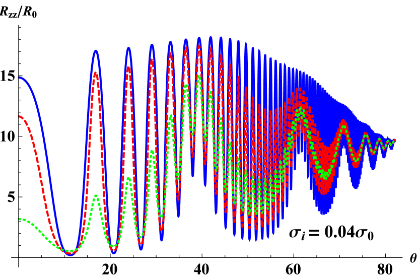
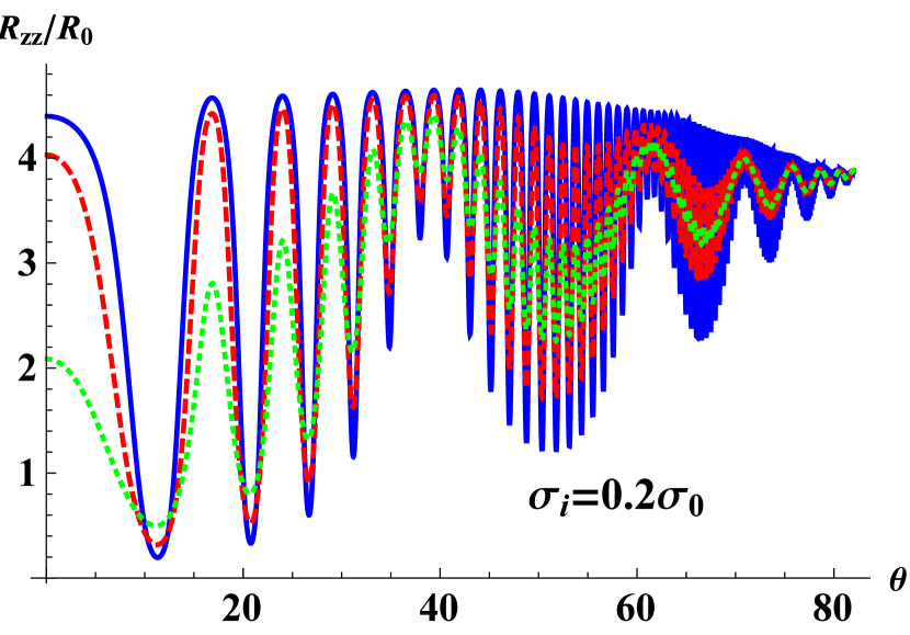
Figure 4: (Color on-line) The angular dependence of magnetoresistance in the presence of incoherent channel of interlayer conductivity at $\sigma^{i}_{zz}=0.04\sigma_{0}$ (Fig. a) and $\sigma^{i}_{zz}=0.2\sigma_{0}$ (Fig. b) for three temperatures $T=0.1\Gamma_{0}$ (blue solid line), $T=0.5\Gamma_{0}$ (red dashed line), and $T=\Gamma_{0}$ (green dotted line).

The long-range disorder, which have the length scale greater than the magnetic length, affects the MQO amplitude differently from the short-range disorder.Raikh The macroscopic sample inhomogeneities locally shift the Fermi level and damp the MQO similar to the temperature smearing of the Fermi level. However, this type of disorder keeps the AMRO amplitude unchanged, similar to the amplitude of the so-called slow oscillations of magnetoresistance.SO ; Shub Using these slow oscillations in organic metals it was shownSO that the contribution $T_{D}^{inh}$ of such sample inhomogeneities to the total Dingle temperature $T_{D}$ of MQO exceeds more than four times the contribution $T_{D}^{*}$ to the Dingle temperature from the short-range disorder. This information is helpful to understand the nature of disorder in various compounds. The observation of slow oscillations requires that the Landau-level separation $\hbar\omega_{c}$ is less than the interlayer transfer integral $t_{z}$ but exceeds the Dingle temperature, i.e. $t_{z}>\hbar\omega_{c}>\Gamma_{0}$. In very anisotropic compounds, where $t_{z}\lesssim\Gamma_{0}$, this condition cannot be satisfied, and the slow oscillations are very difficult to observe. However, just in this limiting case the comparison of the amplitudes of AMRO and MQO allows to determine the contribution $T_{D}^{inh}$ of these sample inhomogeneities from experimental data on magnetoresistance, because the amplitude of AMRO is not affected by $T_{D}^{inh}$ contrary to the amplitude of MQO. The observation of false spin zeros in the amplitude of MQO and their temperature evolution increases the accuracy of such extraction of various contributions to the Dingle temperature from experimental data.

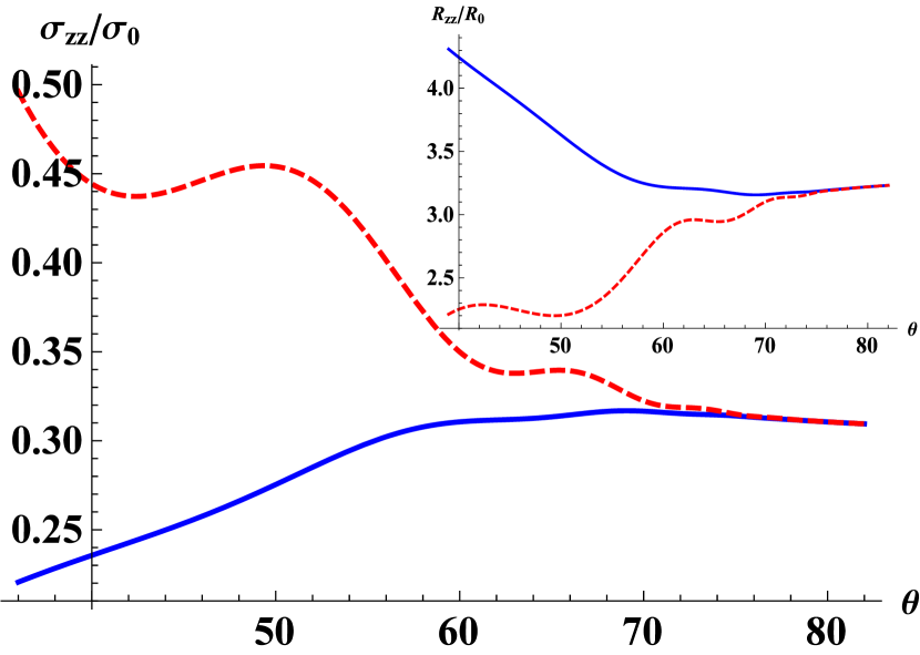
Figure 5: (Color on-line) The maxima (solid blue line) and minima (dashed red line) of quantum oscillations of interlayer conductivity (main panel) and of magnetoresistance (insert figure) calculated in SCBA in the absence of electron reservoir as function of the tilt angle $\theta$ of magnetic field at $k_{F}d=3$ and $\gamma_{0}=2$. These plots give the angular dependence of the envelope of MQO.

III.2 Conductivity in the absence of electron reservoir

In the absence of electron reservoir the electron Green’s function and self-energy are given by Eqs. (29)-(32). In this limit, to calculate conductivity one needs to solve the self-consistency equation (31) for the self energy, which can be done only numerically. In the minima and maxima of MQO of conductivity Eq. (31) simplifies to Eqs. (33) and (34) correspondingly, which are convenient to calculate the envelope of MQO, shown in Fig. 5 for $k_{F}d=3$ and $\gamma_{0}=\pi/\omega_{c}\tau_{0}=2$. In Fig. 6 we plot the normalized amplitude of MQO of conductivity $\left(\sigma_{zz}^{\max}-\sigma_{zz}^{\min}\right)/\sigma_{0}$ for $k_{F}d=3$ and for various values of $\gamma_{0}$. In Fig. 7 we plot the normalized amplitude of MQO of conductivity $\left(\sigma_{zz}^{\max}-\sigma_{zz}^{\min}\right)/\sigma_{0}$ for $\gamma_{0}=3$ and for various values of $k_{F}d$. These plots show that the false spin zeros are more pronounced at larger $k_{F}d$, when AMRO are faster, and are easier observed at $\gamma_{0}<4$. Note, that in both limiting cases, i.e. at large and at zero electron reservoir, the proposed "false spin zeros" only decrease the amplitude of MQO but do not produce the phase inversion of MQO. Thus, contrary to the true spin zeros, given by the factor $R_{s}$ in Eq. (8), which changes the sign and thus leads to the phase shift of MQO by $\pi$, the false spin zeros are not strong enough to make such inversion of MQO. This difference can be used to distinguish between the true and the false spin zeros on experimental data.

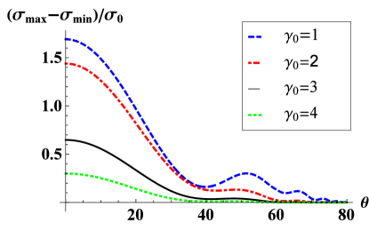
Figure 6: (Color on-line) Angular dependence of relative amplitude $\left(\sigma_{zz}^{\max}-\sigma_{zz}^{\min}\right)/\sigma_{0}$ of the oscillations of interlayer conductivity at $k_{F}d=3$ for various $\gamma_{0}$ calculated in SCBA in the absence of electron reservoir.

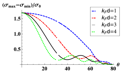
Figure 7: (Color on-line) Angular dependence of relative amplitude $\left(\sigma_{zz}^{\max}-\sigma_{zz}^{\min}\right)/\sigma_{0}$ of oscillations of interlayer conductivity for various $k_{F}d$ at $\gamma_{0}=3$ calculated in SCBA.

IV Conclusions

In this paper we analyze the influence of the angular oscillations of magnetoresistance (AMRO) in quasi-2D metals on its quantum oscillations. We show that the previous assumption of factorization of these two types of oscillations, given by Eq. 4 and usually applied to analyze experimental data, violates in high magnetic field when $\omega_{c}\tau\gtrsim 1$. The strongest violation of Eq. 4 is near the Yamaji angles (AMRO maxima), where the amplitude of MQO is strongly reduced. This interplay of AMRO and MQO at $\omega_{c}\tau\gtrsim 1$ leads to the new qualitative effect – the oscillations (beats) of the amplitude of MQO as function of the tilt angle $\theta$ of magnetic field. These angular minima of MQO amplitude, originating from AMRO and called "false spin zeros", may be erroneously treated as true spin zeros and lead to the incorrect determination of the electron g-factor from MQO. The proposed false spin zeros do not produce the phase inversion of MQO and thus can be distinguished from the true spin zeros. The false spin zeros are more pronounced at larger values of $\omega_{c}\tau$ (see Fig. 6) and at larger values of $k_{F}d$, when AMRO have larger frequency (see Fig. 7). The incoherent channels of interlayer conductivity also make the proposed effect of "false spin zeros" stronger, which is seen from the comparison shown in Figs. 3 and 4. The false spin zeros may help to determine the contribution of such incoherent channel to the total interlayer conductivity from experimental data. The comparison of the amplitude of angular and quantum oscillations may help to determine the nature of disorder which contributes to the Dingle temperature.

Appendix A The two-layer model

In this appendix we remind the formulation and basic formulas of the two-layer model for interlayer conductivity, developed in Refs. TarasPRB2014 ; MosesMcKenzie1999 ; WIPRB2011 . The one-electron Hamiltonian in layered metals with small interlayer coupling consists of the 3 terms

$$\hat{H}=\hat{H}_{0}+\hat{H}_{t}+\hat{H}_{I}.$$ (36)

The first term $\hat{H}_{0}$ is the 2D free electron Hamiltonian summed over all layers $j$ and all quantum numbers $\left\{m\right\}$ of electrons in magnetic field on a 2D conducting layer:

$$\hat{H}_{0}=\sum_{m,j}\epsilon_{2D}\left(m\right)c_{m,j}^{+}c_{m,j},$$

where $\epsilon_{2D}\left(m\right)=\epsilon_{n}=\hbar\omega_{c}\left(n+1/2\right)$ is the corresponding free electron dispersion, and $c_{m}^{+}(c_{m})$ are the electron creation (annihilation) operators in the state $\left\{m\right\}$. The second term in Eq. (36) gives the coherent electron tunnelling between two adjacent layers:

$$\hat{H}_{t}=2t_{z}\sum_{j}\int d^{2}{\boldsymbol{r}}[\Psi_{j}^{\dagger}({\boldsymbol{r}})\Psi_{j-1}({\boldsymbol{r}})+\Psi_{j-1}^{\dagger}({\boldsymbol{r}})\Psi_{j}({\boldsymbol{r}})],$$ (37)

where $\Psi_{j}(x,y)$ and $\Psi_{j}^{\dagger}(x,y)$ are the creation (annihilation) operators of an electron on the layer $j$ at the point $(x,y)$. This interlayer tunnelling Hamiltonian is called "coherent" because it conserves the in-plane electron momentum during the interlayer tunnelling. The last term $\hat{H}_{I}$ is the impurity potential $V_{i}\left(\mathbf{r}\right)$, e.g. given by Eq. (22).

In the strongly anisotropic almost 2D limit, $t_{z}\ll\Gamma,\hbar\omega_{c}$, the interlayer hopping $t_{z}$ can be considered as a perturbation for the periodic stack of uncoupled 2D metallic layers. The interlayer conductivity $\sigma_{zz}$, associated with the Hamiltonian (37), can be calculated using the Kubo formula as a tunnelling conductivity between two adjacent conducting layers $j$ and $j+1$: MosesMcKenzie1999 ; WIPRB2011

$$\sigma_{zz} = \frac{4e^{2}t_{z}^{2}d}{\pi\hbar}\int d\varepsilon\left[-n_{F}^{\prime}(\varepsilon)\right]\int d^{2}{\boldsymbol{r}}\left\langle ImG({\boldsymbol{r}},j,\varepsilon)\right\rangle$$ (38)

$$\times\left\langle ImG(-{\boldsymbol{r}},j+1,\varepsilon)\right\rangle,$$

where the electron Green’s function $G({\boldsymbol{r}},j,\varepsilon)$ on the metallic layer $j$ includes the scattering by impurities. The angular brackets in Eq. (38) mean averaging over impurity configurations. Assuming the impurity distributions on adjacent layer are uncorrelated, the impurity averaging for each Green’s function in Eq. (38) is performed independently.CommentAv Then the averaged Green’s function depends only on the difference ${\boldsymbol{r}}$ of the two coordinates: $\left\langle G({\boldsymbol{r}}_{1},{\boldsymbol{r}}_{2},j,\varepsilon)\right\rangle=\left\langle G({\boldsymbol{r}},j,\varepsilon)\right\rangle$, where ${\boldsymbol{r}}={\boldsymbol{r}}_{2}-{\boldsymbol{r}}_{1}$.

The AMRO of interlayer conductivity in Eq. (38) appear because in a magnetic field $B=\left(B_{x},0,B_{z}\right)=\left(B\sin\theta,0,B\cos\theta\right)$, tilted by the angle $\theta$ to the normal to conducting layers, the Green’s functions on two adjacent layers acquire the phase shift (see Eq. (49) of Ref. MosesMcKenzie1999 ):

$$G_{R}({\boldsymbol{r}},j+1,\varepsilon)=G_{R}({\boldsymbol{r}},j,\varepsilon)\exp\left\{ie\Lambda\left({\boldsymbol{r}}\right)/\hbar\right\},$$ (39)

where

$$\Lambda\left({\boldsymbol{r}}\right)=-yB_{x}d=-yBd\sin\theta.$$ (40)

In the so-called ”non-crossing” approximation, where the electron self-energy contains only diagrams without intersections of impurity lines, the averaged Green’s function on each layer factorizes to (see Appendix in Ref. WIPRB2011 for the proof)

$$G({\boldsymbol{r}}_{1},{\boldsymbol{r}}_{2},\varepsilon)=\sum_{n,k_{y}}\Psi_{n,k_{y}}^{0\ast}(\boldsymbol{r}_{2})\Psi_{n,k_{y}}^{0}(\boldsymbol{r}_{1})G\left(\varepsilon,n\right).$$ (41)

Then the integration over ${\boldsymbol{r}}$ in Eq. (38) can be performed analytically and givesTarasPRB2014 Eqs. (12) and (14).

References

- (1) Shoenberg D. ”Magnetic oscillations in metals”, Cambridge University Press 1984.
- (2) A.A. Abrikosov, Fundamentals of the theory of metals, North-Holland, 1988.
- (3) J. M. Ziman, Principles of the Theory of Solids, Cambridge Univ. Press 1972.
- (4) M.V. Kartsovnik, P. A. Kononovich , V. N. Laukhin and I. F. Shchegolev, JETP Lett. 48, 541 (1988).
- (5) K. Yamaji, J. Phys. Soc. Jpn. 58, 1520 (1989).
- (6) M. V. Kartsovnik, Chem. Rev. 104, 5737 (2004).
- (7) J. Singleton, Rep. Prog. Phys. 63, 1111 (2000).
- (8) M. V. Kartsovnik and V. G. Peschansky, Low Temp. Phys. 31, 185 (2005) [Fiz. Nizk. Temp. 31, 249 (2005)].
- (9) T. Ishiguro, K. Yamaji and G. Saito, Organic Superconductors, 2nd Edition, Springer-Verlag, Berlin, 1998.
- (10) J. Wosnitza, Fermi Surfaces of Low-Dimensional Organic Metals and Superconductors (Springer-Verlag, Berlin, 1996);
- (11) J. S. Brooks, V. Williams, E. Choi1, D. Graf, M. Tokumoto, S. Uji, F. Zuo, J. Wosnitza, J. A. Schlueter, H. Davis, R. W. Winter, G. L. Gard and K. Storr, New Journal of Physics 8, 255 (2006).
- (12) “The Physics of Organic Superconductors and Conductors”, ed. by A. G. Lebed (Springer Series in Materials Science, V. 110; Springer Verlag Berlin Heidelberg 2008).
- (13) M. Kuraguchi et al., Synth. Met. 133-134, 113 (2003).
- (14) C. Bergemann, A. P. Mackenzie, S. R. Julian, D. Forsythe, and E. Ohmichi, Adv. Phys. 52, 639 (2003).
- (15) U. Beierlein, C. Schlenker, J. Dumas, and M. Greenblatt, Phys. Rev. B 67, 235110 (2003)
- (16) N. E. Hussey, M. Abdel-Jawad, A. Carrington, A. P. Mackenzie and L. Balicas, Nature 425, 814 (2003).
- (17) M. Abdel-Jawad, M. P. Kennett, L. Balicas, A. Carrington, A. P. Mackenzie, R. H. McKenzie & N. E. Hussey, Nature Phys. 2, 821 (2006).
- (18) M. Abdel-Jawad, J. G. Analytis, L. Balicas et al., Phys. Rev. Lett. 99, 107002 (2007).
- (19) Malcolm P. Kennett and Ross H. McKenzie, Phys. Rev. B 76, 054515 (2007).
- (20) M. V. Kartsovnik, T. Helm, C. Putzke, F. Wolff-Fabris, I. Sheikin, S. Lepault, C. Proust, D. Vignolles, N. Bittner, W. Biberacher, A. Erb, J. Wosnitza and R. Gross, New Journal of Physics 13, 015001 (2011).
- (21) Sylvia K. Lewin and James G. Analytis, Phys. Rev. B 92, 195130 (2015).
- (22) M. V. Kartsovnik, V. N. Laukhin, S. I. Pesotskii, I. F. Schegolev, V. M. Yakovenko, J. Phys. I 2, 89 (1992).
- (23) M. S. Nam, S. J. Blundell, A. Ardavan, J. A. Symington and J. Singleton, J. Phys.: Condens. Matter 13, 2271 (2001).
- (24) C. Bergemann, S. R. Julian, A. P. Mackenzie, S. NishiZaki, and Y. Maeno, Phys. Rev. Lett. 84, 2662 (2000).
- (25) P.D. Grigoriev, Phys. Rev. B 81, 205122 (2010).
- (26) R. Yagi, Y. Iye, T. Osada, S. Kagoshima, J. Phys. Soc. Jpn. 59, 3069 (1990).
- (27) Yasunari Kurihara, J. Phys. Soc. Jpn. 61, 975 (1992).
- (28) In Q2D metals with dispersion in Eq. (1) and the interlayer conductivity in addition to MQO has the so-called slow oscillationsSO ; Shub ; GKM ; SinchenkoSO with frequency determined by interlayer hopping integral rather than FS cross-section area.
- (29) P.D. Grigoriev, M.M. Korshunov, T.I. Mogilyuk, J. Supercond. Nov. Magn. 29, 1127 (2016).
- (30) A. A. Sinchenko , P. D. Grigoriev, P. Monceau, P. Lejay, V. N. Zverev, J. Low Temp. Phys. 185, 657 (2016); P.D. Grigoriev, A.A. Sinchenko, P. Lejay, A. Hadj-Azzem, J. Balay, O. Leynaud, V.N. Zverev, P. Monceau, Eur. Phys. J. B 89, 151 (2016).
- (31) The electron -factor in metals may differ from the free-electron -factor because of electron interaction, and in non-magnetic compounds -factor is almost independent of .
- (32) V. M. Gvozdikov, Fiz. Tverd. Tela (Leningrad) 26, 2574 (1984) [Sov. Phys. Solid State 26, 1560 (1984)]; T. Champel and V. P. Mineev, Phil. Magazine B 81, 55 (2001).
- (33) P.D. Grigoriev, M.V. Kartsovnik, W. Biberacher, N.D. Kushch, P. Wyder, Phys. Rev. B 65, 060403(R) (2002).
- (34) M.V. Kartsovnik, P.D. Grigoriev, W. Biberacher, N.D. Kushch, P. Wyder, Phys. Rev. Lett. 89, 126802 (2002).
- (35) P.D. Grigoriev, Phys. Rev. B 67, 144401 (2003); arXiv:cond-mat/0204270.
- (36) T. Champel and V. P. Mineev, Phys. Rev. B 66 ,195111 (2002).
- (37) P.D. Grigoriev, T.I. Mogilyuk, Phys. Rev. B 90 , 115138 (2014).
- (38) P. Moses and R.H. McKenzie, Phys. Rev. B 60, 7998 (1999).
- (39) P.D. Grigoriev, Phys. Rev. B 83, 245129 (2011).
- (40) P.D. Grigoriev, Phys. Rev. B 88, 054415 (2013).
- (41) M. E. Raikh and T. V. Shahbazyan, Phys. Rev. B 47, 1522 (1993).
- (42) I.V. Kukushkin, S.V. Meshkov and V.B. Timofeev, Sov. Phys. Usp. 31, 511 (1988) [Usp. Fiz. Nauk 155, 219 (1988)].
- (43) I. L. Aleiner and L. I. Glazman, Phys. Rev. B 52, 11296 (1995). Even in the limit , when the e-e interaction is screened, it affects the g-factor.
- (44) Tsunea Ando, J. Phys. Soc. Jpn. 36, 1521 (1974).
- (45) A. D. Grigoriev, P. D. Grigoriev, Low Temp. Phys. 40, 377 (2014).
- (46) P.D. Grigoriev, JETP Lett. 94, 47 (2011).
- (47) P. Grigoriev, JETP 92, 1090 (2001) [Zh. Eksp. Teor. Fiz. 119(6), 1257 (2001)].
- (48) T. Champel, Phys. Rev. B 64, 054407 (2001).
- (49) A. A. Abrikosov, Physica C 317-318, 154 (1999).
- (50) D. B. Gutman and D. L. Maslov, Phys. Rev. Lett. 99 , 196602 (2007) ; Phys. Rev. B 77, 035115 (2008).
- (51) M. V. Kartsovnik, P. D. Grigoriev, W. Biberacher, and N. D. Kushch, Phys. Rev. B 79, 165120 (2009).
- (52) Urban Lundin and Ross H. McKenzie, Phys. Rev. B 68, 081101(R) (2003).
- (53) A. F. Ho and A. J. Schofield, Phys. Rev. B 71, 045101 (2005).
- (54) The separate averaging of the spectral functions in Eq. ( 38) also assumes the neglection of vertex correctionsMahan in the Kubo formula. The vertex corrections to the interlayer conductivity in Eq. (38) are negligibly small because they contain the product of the electron wave functions on adjacent layers, which is small by the factor . In normal 3D metals the vertex corrections on point-like impurities also vanish; they lead to the replacement of the mean scattering time by the transport mean scattering time,Mahan and these two times coincide for scattering on point-like impurities.
- (55) G. Mahan ”Many-Particle Physics”, 2nd ed., Plenum Press, New York, 1990.