Conventional and unconventional photon statistics

Abstract

We show how the photon statistics emitted by a large variety of light-matter systems under weak coherent driving can be understood, to lowest order in the driving, in the framework of an admixture of (or interference between) a squeezed state and a coherent state, with the resulting state accounting for all bunching and antibunching features. One can further identify two mechanisms that produce resonances for the photon correlations: i) conventional statistics describes cases that involve a particular quantum level or set of levels in the excitation/emission processes with interferences occurring to all orders in the photon numbers, while unconventional statistics describes cases where the driving laser is far from resonance with any level and the interference occurs for a particular number of photons only, yielding stronger correlations but only for a definite number of photons. Such an understanding and classification allows for a comprehensive and transparent description of the photon statistics from a wide range of disparate systems, where optimum conditions for various types of photon correlations can be found and realized.

I Introduction

Quantum optics was born with the study of photon statistics glauber06a . Following Hanbury Brown’s discovery of photon bunching hanburybrown52a ; hanburybrown56c and Kimble et al.’s observation of antibunching kimble77a , there has been a burgeoning activity of tracking how pairs of detected photons are related to each other. From the various mechanisms that generate correlated photons, one that turns an uncorrelated stream into antibunched photons has attracted much attention across different platforms for its practicality of operation (with a laser) and appealing underlying mechanism imamoglu94a ; werner99a ; kim99a ; michler00a ; birnbaum05a ; faraon08a ; dayan08a ; lang11a ; hoffman11a . This so-called “blockade” effect describes how the occupation of an energy level by a particle forbids another particle to occupy the same level. At such, it is reminiscent of Pauli’s exclusion principle kaplan_book16a ; massimi_book05a and indeed the first type of blockade involved electron in the so-called “Coulomb blockade” averin86a ; fulton87a ; kastner08a . However, while Pauli’s principle relies on the antisymmetry of fermionic wavefunctions, one can also implement a “bosonic blockade” with photons exciting an anharmonic system carusotto01a , based on nonlinearities in the energy levels due to self-interactions. The idea is simple: when photons are resonant with the frequency of the oscillator, a first photon can excite the system, but due to photon-photon interactions, a subsequent photon is now detuned from the oscillator’s frequency. If its energy is not sufficient to climb the ladder of states, it cannot excite the system, that remains with one photon. In this way, one can turn a coherent—that is, uncorrelated—stream of photons, with its characteristic Poissonian fluctuations, into a more ordered stream of separated photons, effectively acting as a “photon turnstile”. The quality of such a suppression of the Poisson bursts can be measured at the two-photon level with Glauber’s second-order correlation function $g^{(2)}(\tau)$, that compares the coincidences in time to those expected from a random process of same intensity. Correlations decrease from 1, with no blockade, towards 0 as the nonlinearity $U$ increases. In the limit where $U$ becomes infinite, putting the second excited state arbitrarily far and realizing a two-level system (2LS), a second photon is strictly forbidden and $g^{(2)}$ becomes perfectly antibunched. For open bosonic systems, the ratio of the interaction to the decay rate is an important variable for the blocking to be effective. The “blockade” regime is reached when interactions start to dominate the dissipation. This can be marked as the onset of antibunching: one photon starts to suppress the next one sanvitto19a .

The driven damped anharmonic system is an important model, not least because it is one of the few cases to enjoy an exact analytical solution drummond80a . While much of the mechanism is contained in this particular case, compound systems—where the anharmonic system is coupled to a single-mode cavity—have also attracted considerable attention. This describes for instance interacting quantum-well excitons coupled to a microcavity mode kavokin_book17a . The effect is then known as “polariton-blockade”, after the eponymous light-matter particles that constitute the elementary excitations of such systems. This configuration was first addressed theoretically by Verger et al. verger06a who studied the response of the cavity around the lower-polariton resonance, predicting antibunching indeed, although of too small magnitude with the parameters of typical systems to be observed easily. This spurred interest in polariton boxes and other ways of confining polaritons to enhance their interactions eldaif06a . A few years later, Liew and Savona computed a much stronger antibunching from a seemingly distinct compound system with the same order of nonlinearity, namely, coupled cavities liew10a . This so-called “unconventional polariton blockade” was quickly understood as originating not from the particular configuration of coupled cavities with weak Kerr nonlinearities but from a subtler type of blocking, due to destructive interferences between probability amplitudes whenever there are two paths that can reach the excited state with two photons bamba11a . This result has generated considerable attention, although it was later remarked lemonde14a that it was a known effect carmichael85a ; carmichael91b , observed decades earlier foster00a where it received a much smaller followup. Besides, Lemonde et al. lemonde14a further clarified how unconventional photon blockade is connected to squeezing rather than single-photon states, which had been presented as one of the main interest of the effect. Recently, both conventional arXiv_delteil18a ; arXiv_munozmatutano17a and unconventional vaneph18a ; snijders18a blockades have been reported in solid-state systems, where the 2010 revival of the idea had triggered intense activity.

In this text, we provide a unifying picture of the two types of polariton blockades. We show how they typically sit next to each other in interacting coupled light-matter systems along with other phenomenologies, that produce superbunching instead of the blockade antibunching. In particular, we show that they are both rooted in the single-component system, either a 2LS or an anharmonic oscillator, with strong photon correlations produced by interfering the emitter’s incoherent signal with a coherent fraction. We will nevertheless highlight how the two blockades are intrinsically different mechanisms with different characteristics. Most importantly, the conventional blockade, based on dressed-state blocking, yields photon antibunching at all orders in the number of photons, i.e., $g^{(N)}\rightarrow 0$ for all $N\geq 2$, while the unconventional blockade can only target one $N$ in isolation, producing bunching for the others. Another apparent similarity is that both types of blockades produce the same state in what concerns the population and the two-photon correlation $g^{(2)}$ at the lowest order in the driving, but differences occur at higher orders, namely, at the second-order for $g^{(2)}$ and at the third-order for the population. Differences exist already at the lowest order in the driving for $g^{(3)}$ and higher-order photon correlations, making it clear that the two mechanisms differ substantially and produce different states, despite strong resemblances in the quantities of easiest experimental reach. The state produced by both types of blockade at the two-photon level results from a simple interference between a squeezed state and a coherent state. While the squeezing is typically produced by the emitter, the coherent fraction can be either brought from outside, idoneously, as a fraction of the driving laser itself—a technique known as “homodyning”—or be produced internally by the driven system itself, a concept introduced in the literature under the apt qualification of “self-homodyning” carmichael85a . We will thus highlight that, to this order, essentially the same physics—of tailoring two-photon statistics by admixing squeezed and coherent light, discussed in Section III—takes place in a variety of platforms, overviewed in Section II. We will further synthesize this picture by unifying the cases where the nonlinearity is i) strong, namely, provided by a 2LS (Section IV) or on the contrary ii) weak, namely, provided by an anharmonic oscillator (Section V), and how these are further generalized in presence of a cavity where self-homodyning becomes a compelling picture since a cavity is an ideal receptacle for coherent states. This brings the 2LS into the Jaynes-Cummings model (Section VI) and the anharmonic oscillator into microcavity polaritons (Section VII), respectively. There are many variations in between all these configurations, that the literature has touched upon in many forms, as we briefly overview in the next Section. For our own discussion, while we have tried to retain as much generality as possible for the variables that play a significant role, we do not include for the sake of brevity all the possible combinations, which could of course be done would the need arise for a given platform. Section VIII summarizes and concludes.

II A short review of blockades and related effects

We will keep this overview very short since a thorough review would require a full work on its own. A good review is found in Ref. flayac17b . This Section will also allow us to introduce the formalism and notations. For details of the microscopic derivation, we refer to Ref. verger06a .

A fairly general type of photon blockade is described by the Hamiltonian

$$H={} \hbar\omega_{a}{a^{\dagger}}a+\hbar\omega_{b}{b^{\dagger}}b+\hbar g({a^{\dagger}}b+a{b^{\dagger}})$$ (1a)

$$+\frac{U_{a}}{2}{a^{\dagger}}{a^{\dagger}}aa+\frac{U_{b}}{2}{b^{\dagger}}{b^{\dagger}}bb$$ (1b)

$$+\Omega_{a}e^{i\varpi_{a}t}a+\Omega_{b}e^{i\varpi_{b}t}b$$ (1c)

$$+\mathrm{h.c.}$$

where $\hbar\omega_{c}$ is the free energy of the modes $c=a,b$, both bosonic, $\hbar g$ describes their Rabi coupling, giving rise to polaritons as eigenstates of line (1a), $U_{c}$ are the nonlinearities of the respective modes, here again for $c=a,b$, and $\Omega_{c}$ describes resonant excitation at the energy $\varpi_{c}$. This is brought to the dissipative regime through the standard techniques of open quantum systems, namely, with a master equation in the Lindblad form $\partial_{t}\rho=i\left[\rho,H\right]+\sum_{c=a,b}(\gamma_{c}/2)\mathcal{L}_{c}\rho$, where the superoperator $\mathcal{L}_{c}\rho\equiv 2c\rho{c^{\dagger}}-{c^{\dagger}}c\rho-\rho{c^{\dagger}}c$ describes a decay rate of mode $c$ at rate $\gamma_{c}$ (we do not include incoherent excitation nor dephasing, which are other parameters one could easily account for in the following analysis from a mere technical point of view).

Particular cases or variations of Eq. (1) have been studied in a myriad of works, even when restricting to those with a focus on the emitted photon statistics. This ranges from cases retaining one mode only ferretti12a to the most general form of Eq. (1) ferretti10a ; ferretti13a ; flayac13a ; flayac16a ; flayac17a ; arXiv_liang18a with further variations (such as using pulsed excitation flayac15a ). A first consideration of the effect of field admixture on the photon statistics was made by Flayac and Savona flayac13a , who found that that the conditions for strong correlations are shifted rather than hampered. This touches upon, in the framework of input/output theory, the mechanisms of mixing fields that we will highlight in the following, where we will show that beyond being altered, correlations can be drastically optimized (becoming exactly zero to first order for antibunching and infinite for bunching). In a later work flayac16a , they further progressed towards fully exploiting homodyning by including a “dissipative, one-directional coupling” term, which allowed them to achieve a considerable improvement of the photon correlations, especially in time, with suppression of oscillations and the emergence of a plateau at small time delays. This is due to the same mechanism than the one we used with identical consequences but in a different context lopezcarreno18b (a two-level system admixed to an external laser). Emphasis should also be given to the bulk of work devoted to related ideas of mixing fields by the Vuc̆ković group, starting with their use of self-homodyning to study the Mollow triplet in a dynamical setting fischer16a . Initially used as a suppression technique to access the quantum emitter’s dynamics by cancelling out the scattered coherent component from their driving laser muller16a ; dory17a , they later appreciated the widespread application of their effect and its natural occurence in other systems fischer18a , where it had passed unnoticed, as well as the benefits of a tunability of the interfering component fischer17a , which they proposed in the form of a partially transmitting element in an on-chip integrated architecture that combines a waveguide with a quantum-dot/photonic-crystal cavity QED platform. As such, they have made a series of pioneering contributions in the effect of homodyning for quantum engineering and optimization, which is promised to a great followup li18a . In the following, we will provide a unified theory of the mixing of coherent and quantum light that has been developed and implemented throughout the recent years by Fischer et al. fischer16a ; fischer18a . The possibility and benefits of an external laser to optimize photon correlations also appeared in a work by Van Regemortel et al. vanregemortel18a , with a foothold in the same ideas. The effect of tuning two types of driving was emphasized by Xu and Li xu14a , who reported among other notable results how changing their ratio can bring the system from strong antibunching to superbunching, an idea which we will revisit from the point of view of interfering fields through (controlled) homodyning or (self-consistent) self-homodyning. Similar ideas have then been explored and extended several times in many variations of the problem zhang14e ; tang15a ; shen15a ; shen15b ; li15c ; xu13a ; xu16a ; wang16b ; wang17a ; cheng17a ; deng17a ; zhou16a ; liu16a ; kryuchkyan16a ; zhou16b ; yu17a which all fit nicely in the wider picture that we will present. The microcavity-polariton configuration with interactions in one mode only (describing quantum well excitons, the other being a cavity mode) has been studied mainly from the (conventional) polariton blockade point of view verger06a ; gerace09a , in which case, the (much stronger) unconventional antibunching has been typically overlooked. We will focus in the following on this case rather than on the possibly more popular two weakly-interacting sites. First, because this allows a direct comparison with the Jaynes–Cumming limit, second, because this configuration became timely following the recent experimental breakthrough with polariton blockade arXiv_delteil18a ; arXiv_munozmatutano17a . Whatever the platform, it needs be also emphasized that while many works have focused on single-photon emission as the spotlight for the effect (which is dubious when antibunching is produced from the unconventional route), others have also stressed different applications or suggested different contextualization, such as phase-transitions ferretti10a or entanglement casteels17a , and there is certainly much to exploit from one perspective or another.

Among other configurations that cannot be accommodated by Eq. (1) as they add even more components, one could mention examples from works that involve additional modes (three in Refs. majumdar12e ; kyriienko14c ; kyriienko14a ), different types of nonlinearity, e.g., $a^{2}{b^{\dagger}}$ in Refs. majumdar13a ; gerace14a ; zhou15a , a four-level system in Ref. bajcsy13a ), two two-level system in a cavity in Ref. radulaski17a and up to the general Tavvis–Cummings model arXiv_trivedi19a , pulsed coherent control of a two-level system in Ref. arXiv_loredo18a , two coupled cavities each containing a two-level system knap11a ; schwendimann12a up to a complete array grujic13a . It seems however clear to us that the phenomenology reported in each of these particular cases would fall within the classification that we will establish in the remaining of the text, i.e., they can be understood as an homodyning effect of some sort.

III Homodyne and self-homodyne interferences

We will return in the rest of this text to such systems as those discussed in the previous Section—all a particular case or a variation of Eq. (1)—to show that the two-photon statistics of their emission can be described to lowest order in the driving by a simple process: the mixing of a squeezed and a coherent state. In this Section, we therefore study this configuration in details.

We first consider the mixture of any two fields as obtained in one of the output arms of a balanced beam splitter (cf. Fig. 1a), which is fed by a coherent state on one of its arms, with a complex amplitude $\alpha=|\alpha|e^{i\phi}$, and another field of a general nature, described with annihilation operator $d$, on the other arm. The field that leaves the beam splitter is a mixture of the two input fields, whose annihilation operator can be written as $s=\alpha+d$, where we are leaving out the normalization ($1/\sqrt{2}$) and $\frac{\pi}{2}$-phase shift in the reflected light as reasoned in Appendix A. Within this description, any normally-ordered correlator of the resulting field can be expressed in terms of the inputs as

$$\langle s^{\dagger n}s^{m}\rangle=\sum_{p=0}^{n}\sum_{q=0}^{m}\binom{n}{p}\binom{m}{q}\alpha^{*p}\alpha^{q}\langle d^{\dagger n-p}d^{m-q}\rangle\,.$$ (2)

From this expression, we can compute any relevant observable of the mixture. For instance, the total population is

$$\langle n_{s}\rangle\equiv\langle{s^{\dagger}}s\rangle=|\alpha|^{2}+\langle n_{d}\rangle+2\real[\alpha^{*}\langle d\rangle]\,,$$ (3)

with $n_{d}\equiv d^{\dagger}d$. Apart from the sum of both input intensities, there is a contribution (last term) from the first-order interference between the coherent components of each of the fields or mean fields. Similarly, the second-order coherence function, which is defined as

$$g_{s}^{(2)}(\tau) =\lim_{t\rightarrow\infty}\frac{\langle s^{\dagger}(t)(s^{\dagger}s)(t+\tau)s(t)\rangle}{[\langle s^{\dagger}s\rangle(t)]^{2}}\,,$$ (4a)

$$=\frac{\langle s^{\dagger}(s^{\dagger}s)(\tau)s\rangle}{\langle n_{s}\rangle^{2}}\,,$$ (4b)

can be readily obtained from the correlators in Eq. (2). In this text, we omit the time $t$ in all expressions, as it is considered to be large enough for the system to have reached the steady state under the continuous drive, and will also set the delay $\tau=0$, thus focusing on coincidences. This simplifies the notation $g_{s}^{(2)}=g_{s}^{(2)}(t\rightarrow\infty,\tau=0)$. We will also consider $N$-th order coherence functions, also at zero delay: $g_{s}^{(N)}\equiv\langle s^{\dagger N}s^{N}\rangle/\langle s^{\dagger}s\rangle^{N}$.

These correlators can always be written as a polynomial series of powers of the amplitude of the coherent field $\alpha$:

$$g^{(N)}_{s}=\frac{\sum_{k=0}^{2N}c_{k}(\phi)|\alpha|^{k}}{\langle n_{s}\rangle^{2N}}\,,$$ (5)

where $c_{k}(\phi)$ are coefficients that depend on the phase of the coherent field $\phi$, and mean values of the type $\langle d^{\dagger\mu}d^{\nu}\rangle$ with $\mu+\nu\leq N^{2}$. In particular, the 2nd-order correlation function, Eq. (4b), can be rearranged as

$$g^{(2)}_{s}=1+\mathcal{I}_{0}+\mathcal{I}_{1}+\mathcal{I}_{2}\,,$$ (6)

with $\mathcal{I}_{m}\sim|\alpha|^{m}$ mandel82a ; carmichael85a ; vogel91a ; vogel95a , where 1 represents the coherent contribution of the total signal, and the incoherent contributions read

$$\mathcal{I}_{0} =\frac{\langle d^{\dagger 2}d^{2}\rangle-\langle{d^{\dagger}}d\rangle^{2}}{\langle n_{s}\rangle^{2}}\,,$$ (7a)

$$\mathcal{I}_{1} =4\frac{\real[\alpha^{*}(\langle{d^{\dagger}}d^{2}\rangle-\langle{d^{\dagger}}d\rangle\langle d\rangle)]}{\langle n_{s}\rangle^{2}}\,,$$ (7b)

$$\mathcal{I}_{2} =2\frac{\real[{\alpha^{*}}^{2}\langle d^{2}\rangle]-2\real[\alpha^{*}\langle d\rangle]^{2}+|\alpha|^{2}\langle{d^{\dagger}}d\rangle}{\langle n_{s}\rangle^{2}}$$ (7c)

$$=4\Big{[}|\alpha|^{2}\left(\cos^{2}\phi\ \langle{:}X_{d}^{2}{:}\rangle+\sin^{2}\phi\ \langle{:}Y_{d}^{2}{:}\rangle+{}\right.$$

$$\quad\left.{}+\cos\phi\sin\phi\ \langle\{X_{d},Y_{d}\}\rangle\right)-\real[\alpha^{*}\langle d\rangle]^{2}\Big{]}/\langle n_{s}\rangle^{2}\,.$$

Here, the notation “$::$” indicates normal ordering, $\{X_{d},Y_{d}\}=X_{d}Y_{d}+Y_{d}X_{d}$, and $X_{d}=\frac{1}{2}\left({d^{\dagger}}+d\right)$, $Y_{d}=\frac{i}{2}\left({d^{\dagger}}-d\right)$ are the quadratures of the field described with the annihilation operator $d$. Note that there are no explicit terms $\mathcal{I}_{3}$ and $\mathcal{I}_{4}$ because through simplifications these get absorbed in the term $\mathcal{I}_{1}$.

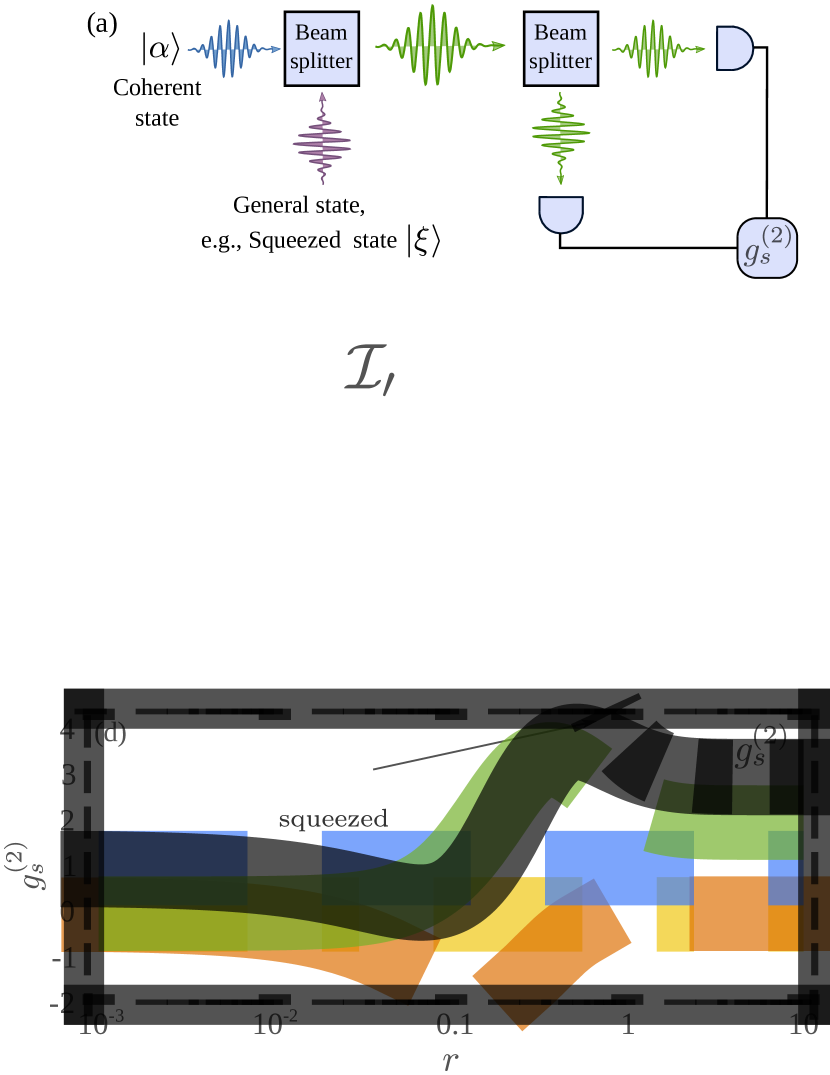
Figure 1: (Color online) Second-order coherence function $g^{(2)}_{s}$ for the interference between a coherent and a quadrature-squeezed field, as in the setup shown in panel (a). The resulting $g^{(2)}_{s}$ is shown in panel (b) as a function of the coherent field $|\alpha|$ and squeezing parameeter $r$ (colour map in log scale). The relative phase between $\phi$ between the squeezed and coherence state is the one that optimises antibunching, i.e., $\phi=\theta/2$. (c) The $n$-norm (up to $g^{(6)}$, i.e., $n=5$) as defined in Eq. (14). Dashed black lines in both panels mark the minimum of $g^{(2)}_{s}$, showing that the best antibunching is no guarantee of good two-photon emission. (d) Cut of $g^{(2)}_{s}$ along the horizontal dashed line in panel (b) ($|\alpha|=0.3$) and its decomposition given by Eqs. (6) and (7). The black dotted line shows $g^{(2)}_{d}$ for the squeezed state only.

The decomposition was, to the best of our knowledge, first introduced by Carmichael carmichael85a and in fact precisely to show that the same quantum-optical phenomenology observed in different systems had the same origin, namely, to root nonclassical effects observed in optical bistability with many atoms in a cavity, to the physics of a single atom coherently driven, i.e., resonance fluorescence. This is at this occasion of unifying squeezing and antibunching from two seemingly unrelated platforms under the same umbrella of self-homodyning that he introduced this terminology. These concepts have thus been invoked and explored to some extent from the earliest days of the field, but it is only recently that they seem to start being fully understood and exploited fischer16a ; flayac16a ; fischer18a ; vanregemortel18a ; lopezcarreno18b . Using such interferences to analyse the squeezing properties of a signal of interest (here, the field with annihilation operator $d$) through a controlled variation of a local oscillator (here, the coherent field $\alpha$), was first suggested by W. Vogel vogel91a ; vogel95a , subsequently implemented to show squeezing in resonance fluorescence schulte15a , and recently impulsed in a series of works from the Vuc̆ković group, as previously discussed. The physical interpretation of the contributions to the decomposition are as follows:

• The numerator of $\mathcal{I}_{0}$ is the normally-ordered variance of the signal intensity, that is, $\langle{:}(\Delta n_{d})^{2}{:}\rangle=\langle{:}n_{d}^{2}{:}\rangle-\langle n_{d}\rangle^{2}$ with $n_{d}=d^{\dagger}d$ and $\Delta n_{d}=n_{d}-\langle n_{d}\rangle$. Therefore, $\mathcal{I}_{0}<0$ indicates that the field $d$ has sub-Poissonian statistics, which in turn contributes to the sub-Poissonian statistics of the total field $s$.

• The numerator of $\mathcal{I}_{1}$ represents the normally-ordered correlation between the fluctuation-field strength and intensity, $\langle{d^{\dagger}}d^{2}\rangle-\langle{d^{\dagger}}d\rangle\langle d\rangle=\langle{:}\Delta d\,\Delta n_{d}{:}\rangle$, which have been referred to as anomalous moments vogel91a ; vogel95a and been recently measured kuhn17a . A squeezed-coherent state has such correlations.

• The numerator of the last component, $\mathcal{I}_{2}$, can also be written in terms of the quadratures of the field $d$. Having $\mathcal{I}_{2}<0$ necessarily implies that the state of light has a squeezing component. This can be proved by noting that ${:}X_{d}^{2}{:}=X_{d}^{2}-1/4$ (the same for ${:}Y_{d}^{2}{:}$). Then, rearranging the numerator of Eq. (7c) leads to:

  $$\langle X_{d,\phi}^{2}\rangle-\langle X_{d_{,}\phi}\rangle^{2}=\left(\Delta X_{d,\phi}\right)^{2}\,,$$ (8)

  where $X_{d,\phi}=(e^{i\phi}{d^{\dagger}}+e^{-i\phi}d)/2$ is the quadrature with the same phase of the coherent field (given by the angle $\phi$). If $\mathcal{I}_{2}<0$, the dispersion of $X_{d,\phi}$ must be less than $1/2$, but since $X_{d,\phi}$ and its orthogonal quadrature, $X_{d,\phi+\pi/2}$, must fulfil the Heisenberg uncertainty relation, $\Delta X_{d,\phi}\Delta X_{d,\phi+\pi/2}\geq 1/4$, then $\Delta X_{d,\phi+\pi/2}>1/2$. This necessarily implies that there is a certain degree of squeezing in $d$. Nevertheless, the opposite statement is not true. A state with a non-zero degree of squeezing can have $\mathcal{I}_{2}\geq 0$, for instance, if the relative direction between the coherent and squeezing contributions fulfils $\theta-2\phi=\pi/2$ (a straightforward example is provided by the displaced squeezed state). Furthermore, if $\langle d\rangle=0$, the numerator of $\mathcal{I}_{2}$ simplifies to $4|\alpha|^{2}(\langle{:}X_{d}^{2}{:}\rangle-|\alpha|^{2})$.

An analogous procedure allows us to decompose the third-order coherence function, $g^{(3)}_{s}=1+\sum_{m=0}^{4}\mathcal{J}_{m}$ (the expressions for $\mathcal{J}_{m}$ are given in Appendix B). Naturally, higher-order-correlator decompositions follow the same rules.

As an illustration which will be relevant in what follows, let us consider the interference between a coherent and a squeezed state, as shown schematically in Fig. 1(a). The coherent state can be written as $\ket{\alpha}=D_{a}(\alpha)\ket{0}$, where $\alpha=|\alpha|e^{i\phi}$ is the amplitude of the coherent state as before, and $D_{a}(\alpha)=\exp(\alpha{a^{\dagger}}-\alpha^{\ast}a)$ is the displacement operator of the field with annihilation operator $a$. Similarly, the squeezed state may be written as $\ket{\xi}=S_{d}(\xi)\ket{0}$, where $\xi=re^{i\theta}$ is the squeezing parameter and $S_{d}(\xi)=\exp(\xi d^{\dagger\,2}-\xi^{\ast}d^{2})$ is the squeezing operator of the field with annihilation operator $d$. Thus, the state that feeds the beam splitter is $\ket{\psi_{\mathrm{in}}}=\ket{\alpha\,,\xi}$. The interference at the beam splitter mixes these two states, and the state of the light that leaves the beam splitter is a two-mode squeezed state that is further squeezed and displaced (the detailed transformation is given in Appendix A). Since we are only interested in the output of one of the arms of the beam splitter, we take the partial trace over the other arm and we end up with a displaced squeezed thermal state lemonde14a ,

$$\rho_{s}=\mathcal{D}_{s}(\alpha)\mathcal{S}_{s}(\xi)\rho_{\mathrm{th}}\left(\langle n_{\mathrm{th}}\rangle\right){\mathcal{S}_{s}^{\dagger}}\left(\xi\right){\mathcal{D}_{s}^{\dagger}}\left(\alpha\right)\,,$$ (9)

where now the displacement and squeezing operators correspond to the operator $s=a+d$, and $\langle n_{\mathrm{th}}\rangle$, the thermal population, can be obtained from the population of the squeezed state, $\langle n_{d}\rangle$, which for a balanced beam splitter follows the relation $\langle n_{\mathrm{th}}\rangle=(\sqrt{1+\langle n_{d}\rangle}-1)/2$. The second-order correlation for the total signal is computed as in Eq. (4), taking the averages using the state in Eq. (9), namely $g^{(2)}_{s}=\Tr[\rho_{s}s^{\dagger\,2}s^{2}]/\Tr[\rho_{s}s^{\dagger}s]^{2}$, which can be decomposed as in Eq. (6) into

$$\mathcal{I}_{0} =\frac{\sinh[4](r)}{\langle n_{s}\rangle^{2}}[1+\coth(r)^{2}]\,,$$ (10a)

$$\mathcal{I}_{1} =0\,,$$ (10b)

$$\mathcal{I}_{2} =\frac{2|\alpha|^{2}\sinh^{2}(r)}{\langle n_{s}\rangle^{2}}\left[1-\cos(\theta-2\phi)\coth(r)\right]\,,$$ (10c)

where $\langle n_{s}\rangle=|\alpha|^{2}+\sinh^{2}(r)$. Here, $\langle d\rangle=0$ but also Eq. (10b) is exactly zero because, for a squeezed state, the correlators $\langle d^{\dagger\mu}d^{\nu}\rangle$ vanish when $\mu+\nu$ is an odd number. Useful expression for the decomposition of $g^{(2)}_{s}$ and $g^{(3)}_{s}$ in terms of the incoherent component and the two-photon coherence are given in Appendix A.

Inspection of Eqs. (10) shows that the only way in which $g^{(2)}_{s}<1$, that is, the statistics of the total signal can be sub-Poissonian, regardless of the value of the squeezing parameter, is for $\mathcal{I}_{2}$ to be negative, which implies that the phases of the displacement and the squeezing must be related by $|\theta-2\phi|<\pi/2$. We take for simplicity the minimizing alignment, $\theta=2\phi$, which means that the coherent and squeezed excitations are driven with the same phase, since the phase of the squeezed state is $\theta/2$. Using such a relation, the interference yields the correlation map shown in Fig. 1(b) as a function of the amplitude of the coherent $|\alpha|$ and squeezing $r$ intensities. The black dashed line shows the optimum amplitude of the coherent state that minimizes $g^{(2)}_{s}$ for a given squeezing, which is given by

$$|\alpha|_{\mathrm{min}}=e^{r}\sqrt{\cosh(r)\sinh(r)}\,.$$ (11)

Replacing this condition in Eqs. (10) we obtain the minimum possible value of $g^{(2)}_{s}$,

$$g_{s,\,\mathrm{min}}^{(2)}=1-\frac{e^{-2r}}{1+\sinh(2r)}\leq 1\,.$$ (12)

This goes to zero although at the same time as the population goes to zero. Figure 1(d) shows a transverse cut of the correlation map in (b) along the purple long-dashed line, which corresponds to $|\alpha|=0.3$. The decomposition and total $g_{s}^{(2)}$ are shown as a function of the squeezing parameter, with minimum $g_{s}^{(2)}=0.26$ at $r\approx 0.078$. Without the interference with the coherent state, the squeezed state can never have sub-Poissonian statistics. In fact, in such a case the correlations become independent of the phase of the squeezing parameter:

$$g^{(2)}_{d}=g_{s}^{(2)}|_{\alpha\rightarrow 0}=2+\coth^{2}(r)\geq 3\,,$$ (13)

which diverges at vanishing squeezing $r\rightarrow 0$ (with also vanishing signal $\langle n_{d}\rangle=\sinh^{2}(r)$), and is minimum when squeezing is infinite $r\rightarrow\infty$.

There is a great tunability from such a simple admixture since $g^{(2)}_{s}$ of the light at the output of the beam splitter can be varied between 0 and $\infty$ simply by adjusting the magnitudes of the coherent field and the squeezing parameter. In particular, the most sub-Poissonian statistics occurs when coherent light interferes with a small amount of squeezing $r<|\alpha_{\mathrm{min}}|$, in the right intensity proportion, given by Eq. (11). Counter-intuitively, $g^{(2)}_{s}\ll 1$ occurs when the squeezed light itself is, on the opposite, super-Poissonian (even super-chaotic $g_{d}^{(2)}>2$) . This is a fundamental result that we will find throughout the text in order to find the conditions for and manipulate sub-Poissonian statistics and antibunching in various systems under weak coherent driving.

An important fact for our classification of photon statistics is that, since the sub-Poissonian behaviour is here due to an interference effect, the set of parameters that suppresses the fluctuation at the two-photon level does not suppress them at all $N$-photon levels, which means that the multi-photon emission cannot be precluded simultaneously at all orders. In other words, the condition in Eq. (11) that minimizes $g_{s}^{(2)}$, also minimizes the two-photon probability in the interference density matrix $\bra{2}\rho_{s}\ket{2}$, at low intensities. But this is not the same condition that minimizes any other photon probability $\bra{n}\rho_{s}\ket{n}$. This incompatibility is revealed by the $n$-norm, as defined in Ref. arXiv_lopezcarreno16c , which is the distance in the correlation space between signal $s$ and a perfect single-photon source:

$$\norm{(g^{(k)}_{s})}_{n}=\sqrt[n]{\sum_{k=2}^{n+1}[g^{(k)}_{s}]^{n}}\,.$$ (14)

In Figure 1(c) we show the $5$-norm for the same range of parameters of Panel (b). The dashed black line indicates the minimum values of $g^{(2)}_{s}$, which lies in a high-fluctuation region when the higher order correlation functions are taken into account. Further increasing $n$ renders the correlation map completely red which means that multiphoton emission is not suppressed even if we have $g^{(2)}_{s}$ close to zero. This is a feature typical of antibunching that arises from a two-photon interference only, that suggests that their use as single-photon sources may be an issue in the context of applications for quantum technology where higher-photon correlations may jeopardize two-photon suppression. This is related to the fact that this antibunching stems from a Gaussian state, which is the most classical of the quantum states.

The discussion presented above and, in particular, the decomposition of the second-order correlation as in Eq. (6), are not limited to the particular case of interfering pure states set as initial conditions. This can also be applied to the dynamical case of a single system which provides itself and directly a coherent component $\alpha$ along with another, and therefore quantum, type of component. Calling $s$ the annihilation operator for a particular emitter which has such a coherent—but not exclusively—component in its radiation, one can thus express its emission as the interference (or superposition) of a mean coherent field $\langle s\rangle$ and its quantum fluctuations, with operator $d=s-\langle s\rangle$. That is, one can always write

$$s=\langle s\rangle+d\,.$$ (15)

Following the terminology previously introduced in the literature for a similar purpose carmichael85a , we call this interpretation of the emission a self-homodyne effect. Since $g_{s}^{(2)}$ is also given by Eq. (7) with the simplification brought by the fact that $\langle d\rangle=0$, by replacing $\alpha\rightarrow\langle s\rangle$ and $d\rightarrow s-\langle s\rangle$, we obtain the general expressions in terms of $\langle s^{\dagger n}s^{m}\rangle$ for the emission of a single-emitter $s$, interfering its own components:

$$\mathcal{I}_{0} =\frac{\langle s^{\dagger 2}s^{2}\rangle-\langle{s^{\dagger}}s\rangle^{2}-4|\langle s\rangle|^{4}+6|\langle s\rangle|^{2}\langle{s^{\dagger}}s\rangle+2\real[{\langle{s^{\dagger}}\rangle}^{2}\langle s^{2}\rangle-2\langle{s^{\dagger}}\rangle\langle{s^{\dagger}}s^{2}\rangle]}{\langle{s^{\dagger}}s\rangle^{2}}\,,$$ (16a)

$$\mathcal{I}_{1} =4\frac{\real[\langle{s^{\dagger}}\rangle\langle{s^{\dagger}}s^{2}\rangle-\langle{s^{\dagger}}\rangle^{2}\langle s^{2}\rangle]+2|\langle s\rangle|^{2}\left(|\langle s\rangle|^{2}-\langle{s^{\dagger}}s\rangle\right)}{\langle{s^{\dagger}}s\rangle^{2}}\,,$$ (16b)

$$\mathcal{I}_{2} =2\frac{\real[\langle{s^{\dagger}}\rangle^{2}\langle s^{2}\rangle]+|\langle s\rangle|^{2}\langle{s^{\dagger}}s\rangle-2|\langle s\rangle|^{4}}{\langle{s^{\dagger}}s\rangle^{2}}\,.$$ (16c)

For completeness, in Appendix C we present the possible models (Hamiltonians and Liouvillians) that produce a coherent state and a squeezed state in a cavity, and give the correspondence between the dynamical parameters (such as the coherent driving and the squeezing intensity) and the abstract quantities $\alpha$ and $r$.

In the following Sections we will use the self-homodyne decomposition Eqs. (16) and this understanding in terms of interferences between coherent and quantum components, which in our cases may or may not be of the squeezing type, to analyse some statistical properties (anti- and super-bunching) of systems in their low-driving regime, and contrast their statistics with conventional blockade effects. We will focus on cases that are both fundamental and tightly related to each other, namely, the 2LS (resonance fluorescence) in Section IV, the anharmonic oscillator in Section V, the Jaynes–Cummings Hamiltonian in Section VI and microcavity polaritons in Section VII.

IV Resonance fluorescence in the Heitler regime

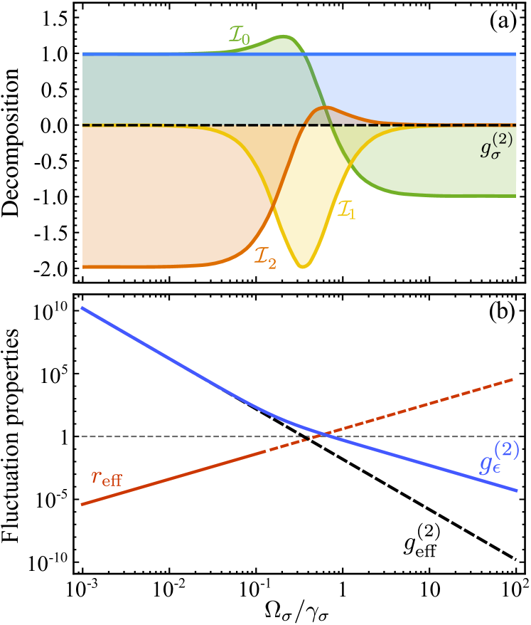
Figure 2: Second-order coherence function $g^{(2)}_{\sigma}$ (dashed black) of resonance fluorescence, as a function of the driving-laser intensity $\Omega_{\sigma}$ (at resonance). The Heitler regime, investigated in this work, is on the left ($\Omega_{\sigma}\ll\gamma_{\sigma}$). (a) Decomposition of $g^{(2)}_{\sigma}$, given by Eq. (16) with $s\rightarrow\sigma$, which cancels out to give an exact zero. (b) Squeezing properties of the emitted light ($\Delta_{\sigma}=0$), characterised by the effective squeezing parameter $r_{\mathrm{eff}}$ (Eq. (35)) for the fluctuations only $\epsilon$ (red line), and statistics of the fluctuations $g^{(2)}_{\epsilon}$ (solid blue line), given by Eq. (23). The latter can be approximated by $g^{(2)}_{\mathrm{eff}}$ (Eq. (38)) when the driving is low enough. The red solid line indicates when the effective squeezing parameter fits properly the actual statistics and becomes dashed when the approximation fails. In both cases, the range of validity is $\Omega_{\sigma}\lesssim 0.1\gamma_{\sigma}$.

We first consider the excitation of a two-level system (2LS) driven by a coherent source in the regime of low excitation—commonly referred to as the Heitler regime. Such a system is modeled by the Hamiltonian ($\hbar=1$)

$$H_{\mathrm{rf}}=(\omega_{\sigma}-\omega_{\mathrm{L}}){\sigma^{\dagger}}\sigma+\Omega_{\sigma}\left({\sigma^{\dagger}}+\sigma\right)\,.$$ (17)

This is the particular case of the general Hamiltonian (1) when only one mode is considered and $U\rightarrow\infty$. Here, the 2LS has a frequency $\omega_{\sigma}$ and is described with an annihilation operator $\sigma$ that follows the pseudospin algebra, whereas the laser is treated classically, i.e., as a complex number, with intensity $\Omega_{\sigma}$ (taken real without loss of generality) and frequency $\omega_{\mathrm{L}}$. The dynamics only depends on the frequency difference, $\Delta_{\sigma}\equiv\omega_{\sigma}-\omega_{\mathrm{L}}$. The dissipative character of the system is included in the dynamics with a master equation $\partial_{t}\rho=i\left[\rho,H_{\mathrm{rf}}\right]+(\gamma_{\sigma}/2)\mathcal{L}_{\sigma}\rho$, where the Lindblad form $\mathcal{L}_{\sigma}\rho=2\sigma\rho{\sigma^{\dagger}}-{\sigma^{\dagger}}\sigma\rho-\rho{\sigma^{\dagger}}\sigma$ describes the decay of the 2LS at a rate $\gamma_{\sigma}$. The steady-state solution (computed as indicated in Appendix D) can be fully written in terms of two parameters: the 2LS population (or probability to be in the excited state) $\langle n_{\sigma}\rangle\equiv\langle{\sigma^{\dagger}}\sigma\rangle$, and the coherence or mean field $\alpha\equiv\langle\sigma\rangle$ delvalle11a :

$$\rho=\begin{pmatrix}1-\langle n_{\sigma}\rangle&\alpha^{\ast}\\ \alpha&\langle n_{\sigma}\rangle\end{pmatrix},$$ (18)

where

$$\langle n_{\sigma}\rangle=\frac{4\Omega_{\sigma}^{2}}{\gamma_{\sigma}^{2}+4\Delta_{\sigma}^{2}+8\Omega_{\sigma}^{2}}\,,$$ (19a)

$$\alpha=\frac{2\Omega_{\sigma}(2\Delta_{\sigma}+i\gamma_{\sigma})}{\gamma_{\sigma}^{2}+4\Delta_{\sigma}^{2}+8\Omega_{\sigma}^{2}}\,.$$ (19b)

As a consequence of the fermionic character of the 2LS, it can only sustain one excitation at a time. Therefore, all the correlators different from those in Eq. (19) vanish, and in particular the $N$-photon correlations of the two-level system are exactly zero, namely $g^{(N)}_{\sigma}=0$ for $N\geq 2$. We call this perfect cancellation of correlations to all orders conventional blockade or conventional antibunching (CA), as it arises from the natural Pauli blocking scenario. To investigate the components of the correlations that ultimately provide the perfect sub-Poissonian behaviour of the 2LS, we separate the mean field from the fluctuations of the signal ($\sigma=\alpha+\epsilon$), in analogy with Eq. (15). Following Eqs. (16), $g^{(2)}_{\sigma}$ can be decomposed as in Eq. (6) with,

$$\mathcal{I}_{0} =\frac{|\alpha|^{2}\left(6\langle n_{\sigma}\rangle-4|\alpha|^{2}\right)}{n_{\sigma}^{2}}-1\,,$$ (20a)

$$\mathcal{I}_{1} =-8\frac{|\alpha|^{2}\left(\langle n_{\sigma}\rangle-|\alpha|^{2}\right)}{n_{\sigma}^{2}}\,,$$ (20b)

$$\mathcal{I}_{2} =2\frac{|\alpha|^{2}\left(\langle n_{\sigma}\rangle-2|\alpha|^{2}\right)}{n_{\sigma}^{2}}\,.$$ (20c)

These are presented in Fig. 2(a) as a function of the intensity of the driving laser. The decomposition shows that, although the photon correlations of the 2LS are always perfectly sub-Poissonian, or antibunched , the nature of their cancellation varies depending on the driving regime lopezcarreno18b . In the high-driving regime, the coherent component is compensated by the sub-Poissonian statistics of the quantum fluctuations ($\mathcal{I}_{0}<0$) since $\lim_{\Omega_{\sigma}\rightarrow\infty}\alpha=0$ and fluctuations become the total field, $\epsilon\rightarrow\sigma$. In contrast, in the Heitler regime the coherent component is compensated by the super-Poissonian but also squeezed fluctuations ($\mathcal{I}_{2}<0$). The Heitler regime is, therefore, an example of the type of self-homodyne interference that we discussed in Sec. III.

Let us then analyse more closely the fluctuations by looking into their correlation functions:

$$\langle\epsilon^{\dagger k}\epsilon^{l}\rangle=(-1)^{k+l}\alpha^{\ast\,k-1}\alpha^{l-1}\big{(}|\alpha|^{2}(1-k-l+kl)+kl\,\langle n_{\epsilon}\rangle\big{)}\,,$$ (21)

where $\langle n_{\epsilon}\rangle=\langle n_{\sigma}\rangle-|\alpha|^{2}$ is the contribution from the fluctuations to the total population of the 2LS. More details are given in Appendix E. In particular, the $N$-photon correlations from the fluctuations alone is given by,

$$g^{(N)}_{\epsilon}=\frac{|\alpha|^{2(N-1)}\big{(}N^{2}\,\langle n_{\sigma}\rangle+(1-2N)|\alpha|^{2}\big{)}}{(\langle n_{\sigma}\rangle-|\alpha|^{2})^{N}}\,,$$ (22)

that in terms of the physical parameters reads

$$g^{(N)}_{\epsilon}=\frac{\left(N-1\right)^{2}\left(\gamma_{\sigma}^{2}+4\Delta_{\sigma}^{2}\right)+8N^{2}\Omega_{\sigma}^{2}}{8^{N}\,\Omega_{\sigma}^{2N}\left(\gamma_{\sigma}^{2}+4\Delta_{\sigma}^{2}\right)^{N-1}}\,.$$ (23)

In Fig. 2(b) we plot $g^{(2)}_{\epsilon}$ confirming that fluctuations are sub-Poissonian or super-Poissonian depending on whether the effective driving defined as $\Omega_{\mathrm{eff}}\equiv\Omega_{\sigma}/\sqrt{1+(2\Delta_{\sigma}/\gamma_{\sigma})^{2}}$ is much larger or smaller than the system decay $\gamma_{\sigma}$, respectively (the figure is for the resonant case).

In the Heitler regime, we need to consider only the magnitudes up to leading order in the effective normalised driving $p\equiv 2\Omega_{\mathrm{eff}}/\gamma_{\sigma}$. The main contribution to the intensity $\langle n_{\sigma}\rangle=|\alpha|^{2}+\langle n_{\epsilon}\rangle$, in the absense of pure dephasing, comes from the coherent part $|\alpha|^{2}$ of the signal. Fluctuations only appear to the next order, having, up to fourth order in $p$:

$$\langle n_{\sigma}\rangle =p^{2}-2p^{4}\,,$$ (24a)

$$|\alpha|^{2} =p^{2}-4p^{4}\,,$$ (24b)

$$\langle n_{\epsilon}\rangle =2p^{4}\,.$$ (24c)

The coherent contribution corresponds to the elastic (also known as “Rayleigh”) scattering of the laser-photons by the two-level system, while the fluctuations originate from the two-photon excitation and re-emission dalibard83a . In the spectrum of emission, this manifests as a superposition of a delta and a Lorentzian peaks with exactly these weights, $|\alpha|^{2}$ and $\langle n_{\epsilon}\rangle$, both centered at the laser frequency, with no width (for an ideal laser) and $\gamma_{\sigma}$-width, respectively mollow69a ; loudon_book00a ; lopezcarreno18b . Fluctuations have no coherent intensity by construction, $\langle\epsilon\rangle=0$. At the same time, their second momentum is not zero but exactly the opposite of the coherent field one: $\langle\epsilon^{2}\rangle=-\alpha^{2}$, thanks to the fact that $\langle\sigma^{2}\rangle=\alpha^{2}+\langle\epsilon^{2}\rangle=0$. This means that both contributions, coherent and incoherent, are of the same order in the driving $p$ when it comes to two-photon processes and can, therefore, interfere and even cancel each other. This is precisely what happens and is made explicit in the $g^{(2)}_{\sigma}$-decomposition above. The strong two-photon interference ($\mathcal{I}_{2}$) can compensate the Poissonian and super-Poissonian statistics of the coherent and incoherent parts of the signal ($1+\mathcal{I}_{0}$). Since quadrature squeezing is created by a displacement operator, or a Hamiltonian, based on the operator $\epsilon^{2}$, this situation corresponds to a high degree of quadrature squeezing for the fluctuations. Further analysis of the fluctuation quadratures (details of the calculation are in Appendix E) shows that their variances behave similarly to a squeezed thermal state in the Heitler regime, which allows us to derive an effective squeezing parameter $r_{\mathrm{eff}}=p^{2}$ to describe the state to lowest order in the driving. This is plotted in Fig. 2(b) as a function of the driving, with the line becoming dashed when the interference can no longer be described in terms of a squeezed thermal state. Note that the total signal has no squeezing at low driving, only fluctuations do, because the coherent contribution is much larger.

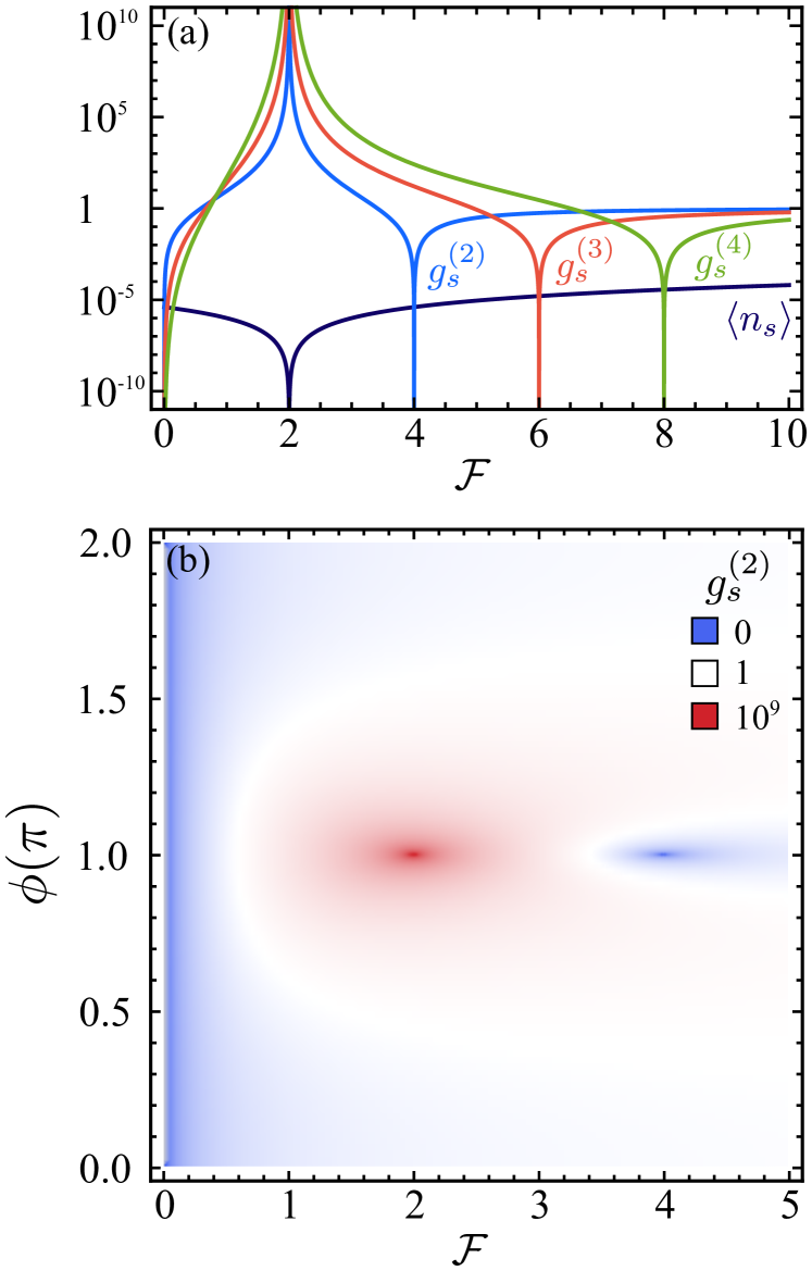
Figure 3: (Color online) Interference between the output of resonance fluorescence and an external laser of intensity proportional to $\mathcal{F}$ and phase $\phi$. All modes at resonance. (a) Intensity $\langle n_{s}\rangle$ and $N$-th order coherence functions $g_{s}^{(N)}$ of the resulting light as a function of $\mathcal{F}$. (b) $g_{s}^{(2)}$ as a function of both $\mathcal{F}$ and $\phi$ (in units of $\pi$) with the colour code in inset (logscale). Tuning the external laser allows to choose between various resonant conditions.

Resonance fluorescence by itself always provides antibunching, due to the perfect cancellation of the various components. However, one can disrupt this by manipulating the coherent fraction, simply by interfering the signal $\sigma$ in a beam splitter with an external coherent state $\ket{\beta}$. This allows to change the photon statistics of the total signal $s=\mathrm{T}\sigma+i\mathrm{R}\beta$, where $T^{2}$ and $R^{2}$ are the transmittance and reflectance of the beam splitter. Actually, since the decomposition affects correlators to all orders, Eq. (22), one can target the $N$-photon level instead of the 2-photon one. Namely, one can decide to set the $N$-photon coherence function to zero. As a particular case, the 1-photon case cancels the signal altogether, which is obtained by solving the condition $\langle n_{s}\rangle=\mathrm{T}^{2}|\alpha+i\mathrm{R}\beta_{1}/\mathrm{T}|^{2}=0$ (because $\langle n_{\epsilon}\rangle=0$ to second order in $\Omega_{\sigma}$). We will show that the possibility to target one $N$ in isolation of the others introduces a separate regime from conventional blockade. Given their relationship and in line with the terminology found in the literature, we refer to this as unconventional blockade and unconventional antibunching (UA).

With this objective of tuning $N$-photon statistics and in order to avoid referencing the specificities of the beam splitter which do not change the normalized observables, let us define $\beta^{\prime}\equiv\mathrm{R}\beta/\mathrm{T}\equiv|\beta^{\prime}|e^{i\phi}$ and parametrise its amplitude as a fraction $\mathcal{F}$ (always a positive number) of the laser field exciting the 2LS:

$$|\beta^{\prime}|=\frac{\Omega_{\sigma}}{\gamma_{\sigma}}\mathcal{F}\,.$$ (25)

With this, the coherence function $g^{(N)}_{s}$ of the interfered field in the Heitler regime is given by:

$$g^{(N)}_{s}=\frac{\mathrm{T}^{2N}}{\langle n_{s}\rangle^{N}}\frac{\mathcal{F}^{2(N-1)}\Omega_{\sigma}^{2N}}{\gamma_{\sigma}^{2N}\left(\gamma_{\sigma}^{2}+4\Delta_{\sigma}^{2}\right)}\times\\ \big{[}\mathcal{F}^{2}\left(\gamma_{\sigma}^{2}+4\Delta_{\sigma}^{2}\right)+4N\mathcal{F}\gamma_{\sigma}\left(\gamma_{\sigma}\cos\phi-2\Delta_{\sigma}\sin\phi\right)+{}\\ {}+4N^{2}\gamma_{\sigma}^{2}\big{]}\,.$$ (26)

Since $g_{s}^{(1)}=1$, this expression also provides the population $\langle n_{s}\rangle$ by considering the case $N=1$. One can appreciate the considerable enrichment brought by the interfering laser by comparing $\langle n_{s}\rangle$ (with the interfering laser, $\mathcal{F}\neq 0$) to Eq. (19(a)) (without, $\mathcal{F}=0$) and even more so by comparing the $N$-photon correlation function, which is identically zero without the interfering laser, and that becomes Eq. (26) with the interfering laser. Interestingly, there is now another condition that suppresses the correlations and yields perfect antibunching at a given $N$-photon order, in addition to the one obtained in the original system without the interfering laser (CA). The new conditions exist for any detuning and are given by:

$$\tan\phi_{N}=-\frac{2\Delta_{\sigma}}{\gamma_{\sigma}}\quad\quad\mathrm{and}\quad\quad\mathcal{F}_{N}=-2N\cos\phi_{N}\,.$$ (27)

Focusing on the resonance case for simplicity, we have $\mathcal{F}_{N}=2N$ and always the same phase, $\phi_{N}=\pi$, which corresponds to the field $i\beta_{N}^{\prime}=-N|\alpha|$. The total coherent fraction changes phase for all $N$: $\alpha+i\beta_{N}^{\prime}=-(N-1)\alpha$. The signal population ($\langle n_{s}\rangle=G^{(1)}_{s}$) vanishes due to a first order (or one-photon) interference at the external laser parameter $\mathcal{F}_{1}=2$, which translates into $i\beta_{1}^{\prime}=-i|\alpha|$. The external laser completely compensates the coherent fraction of resonance fluorescence, in this case $\alpha=i|\alpha|$ (with $|\alpha|=2\Omega_{\sigma}/\gamma_{\sigma}$). This situation corresponds to a classical destructive interference, which equally occurs between two fully classical laser beams with the same intensity and opposite phase.

In the case of highest interest, that of two-photon correlations $g^{(2)}_{s}$, we find a destructive two-photon interference at the intensity $\mathcal{F}_{2}=4$, which corresponds to an external laser $i\beta_{2}=-2|\alpha|$, that fully inverts the sign of the coherent fraction in the total signal: $\alpha+i\beta_{2}^{\prime}=-\alpha$. This coherent contribution leads to perfect cancelation of the two-photon probability in a wavefunction approach visser95a (see the details in Appendix F.2). Note that this does not, however, satisfy all other $N$-photon interference conditions and $g^{(N)}_{s}$ with $N>2$ do not vanish. This is a very different situation as compared to the original resonance fluorescence where $g^{(N)}_{\sigma}=0$ for all $N>1$. One, the conventional scenario, arises from a an interference that takes place at all orders. The other, the unconventional scenario, results from an interference that is specific to a given number of photons.

$g^{(N)}$	Squeezed Thermal	Heitler fluctuations	Displaced Squeezed Thermal	Laser-corrected configuration
$n_{a}$	$\frac{32\Omega_{\sigma}^{4}}{\Gamma_{\sigma}^{4}}+\frac{1792\Omega_{\sigma}^{8}}{3\Gamma_{\sigma}^{8}}+O\left(\Omega_{\sigma}^{12}\right)$	$\frac{32\Omega_{\sigma}^{4}}{\Gamma_{\sigma}^{4}}-\frac{512\Omega_{\sigma}^{6}}{\Gamma_{\sigma}^{6}}+O\left(\Omega_{\sigma}^{8}\right)$	$\frac{4\Omega_{\sigma}^{2}}{\Gamma_{\sigma}^{2}}+\frac{32\Omega_{\sigma}^{4}}{\Gamma_{\sigma}^{4}}+O\left(\Omega_{\sigma}^{6}\right)$	$\frac{4\Omega_{\sigma}^{2}}{\Gamma_{\sigma}^{2}}-\frac{32\Omega_{\sigma}^{4}}{\Gamma_{\sigma}^{4}}+O\left(\Omega_{\sigma}^{6}\right)$
$g^{(2)}$	$\frac{\Gamma_{\sigma}^{4}}{64\Omega_{\sigma}^{4}}+\frac{11}{4}+O\left(\Omega_{\sigma}^{4}\right)$	$\frac{\Gamma_{\sigma}^{4}}{64\Omega_{\sigma}^{4}}+\frac{\Gamma_{\sigma}^{2}}{2\Omega_{\sigma}^{2}}+O\left(\Omega_{\sigma}^{0}\right)$	$0+\frac{32\Omega_{\sigma}^{2}}{\Gamma_{\sigma}^{2}}+O\left(\Omega_{\sigma}^{4}\right)$	$0+\frac{128\Omega_{\sigma}^{2}}{\Gamma_{\sigma}^{2}}+O\left(\Omega_{\sigma}^{4}\right)$
$g^{(3)}$	$\frac{9\Gamma_{\sigma}^{4}}{64\Omega_{\sigma}^{4}}+\frac{51}{4}+O\left(\Omega_{\sigma}^{4}\right)$	$4-\frac{96\Omega_{\sigma}^{2}}{\Gamma_{\sigma}^{2}}+O\left(\Omega_{\sigma}^{4}\right)$	$16+\frac{768\Omega_{\sigma}^{2}}{\Gamma_{\sigma}^{2}}+O\left(\Omega_{\sigma}^{4}\right)$	$\frac{\Gamma_{\sigma}^{6}}{128\Omega_{\sigma}^{6}}+\frac{9\Gamma_{\sigma}^{4}}{64\Omega_{\sigma}^{2}}+O\left({1\over\Omega_{\sigma}^{2}}\right)$

Table 1: Two-level system. Comparison of first- (population), second- and third-order photon correlations, i) between a Squeezed Thermal state and the fluctuations in the Heitler regime and ii) between a Displaced Squeezed Thermal state and the fluctuations in the laser-corrected Heitler regime, to various orders in the driving $\Omega_{\sigma}$.

$g^{(N)}$	Displaced Squeezed Thermal	AO antibunching	Displaced Squeezed Thermal	Laser-corrected configuration
$n_{a}$	$2.89\,\Omega_{b}^{2}+4.63\,\Omega_{b}^{4}+O\left(\Omega_{b}^{6}\right)$	$2.89\,\Omega_{b}^{2}-10.36\,\Omega_{b}^{4}+O\left(\Omega_{b}^{6}\right)$	$1.52\,\Omega_{b}^{2}+4.63\,\Omega_{b}^{4}+O\left(\Omega_{b}^{6}\right)$	$1.52\,\Omega_{b}^{2}-3.25\,\Omega_{b}^{4}+O\left(\Omega_{b}^{6}\right)$
$g^{(2)}$	$0.38+5.18\,\Omega_{b}^{2}+O\left(\Omega_{b}^{4}\right)$	$0.38+0.91\,\Omega_{b}^{2}+O\left(\Omega_{b}^{4}\right)$	$0+12.75\,\Omega_{b}^{2}+O\left(\Omega_{b}^{4}\right)$	$0+47.84\,\Omega_{b}^{2}+O\left(\Omega_{b}^{4}\right)$
$g^{(3)}$	$0.80+1.64\,\Omega_{b}^{2}+O\left(\Omega_{b}^{4}\right)$	$0.06+0.37\,\Omega_{b}^{2}+O\left(\Omega_{b}^{4}\right)$	$4-34.52\,\Omega_{b}^{2}+O\left(\Omega_{b}^{4}\right)$	$0.71+0.78\,\Omega_{b}^{2}+O\left({\Omega_{b}^{4}}\right)$

Table 2: Anharmonic oscillator. Comparison of first- (population), second- and third-order photon correlations, i) between a Displaced Squeezed Thermal state and the anharmonic oscillator with $\Delta_{b}=\Delta_{-}$ (optimal antibunching) and ii) between a Displaced Squeezed Thermal state and the laser-corrected for the optimal $g^{(2)}$ configuration ($\mathcal{F}_{2,2}$ and $\phi_{2,2}$). Selected parameters: $\gamma_{b}=U=1$.

All these interferences can be seen in Fig. 3(a) where we plot them up to $N=4$. When there is no interference with the external laser, $\mathcal{F}=0$, antibunching is perfect to all orders recovering resonance fluorescence. At the one-photon interference, the denominator of $g^{(N)}_{s}$ becomes zero and the functions, therefore, diverge. This produces a superbunching effect of a classical origin, as previously discussed: a destructive interference effect that brings the total intensity to zero. In this case, the external laser removes completely by destructive interference the coherent fraction of the total signal. Therefore, the statistics is that of the fluctuations alone, what we previously called $g^{(N)}_{\mathrm{\epsilon}}$, given by Eq. (22). We have already discussed how, in the Heitler regime, fluctuations become super chaotic and squeezed. We can see, on the left hand side of Fig. 1, that in the limit of $\Omega_{\sigma}\rightarrow 0$, they actually diverge. Such a superbunching is thus linked to noise. The resulting state is missing the one-photon component and, consequently, the next (dominating) component is the two-photon one. Nevertheless, there is not a suppression mechanism for components with higher number of photons so that the relevance of such a configuration for multiphoton (bundle) emission remains to be investigated, which is however better left for a future work. We call this feature unconventional bunching (UB) in contrast with bunching that results from a $N$-photon de-excitation process that excludes explicitly the emission of other photon-numbers. This superbunching, as well as the antibunching by destructive interferences, will be reappearing in the next systems of study. The Heitler regime is, therefore, a simple but rich system where all the squeezing-originated interferences already occur although we need an external laser to have them manifest.

We now turn to the subtle point of which quantum state is realized by the various scenarios. To lowest-order in the driving, the dynamical state of the system can be described by a superposition of a coherent and a squeezed state, insofar as only the lower-order correlation functions (namely, population and $g^{(2)}$) are considered. This is shown in Table 1, where we compare $g^{(N)}$ for $1\leq N\leq 3$ (with $N=1$ corresponding to the population) for the fluctuations in the Heitler regime vs the corresponding observables for a squeezed thermal state, on the one hand, and the laser-corrected configuration vs the displaced squeezed thermal state on the other hand. As explained in Appendix E, such a comparison can be made by identifying the squeezing parameter and thermal populations to various orders in a series expansion of the quantum states with the corresponding observables from the dynamical systems. One finds:

$$\mathrm{r}_{\mathrm{eff}}=\frac{4\Omega_{\sigma}^{2}}{\Gamma_{\sigma}^{2}}, \mathrm{p}_{\mathrm{eff}}=\frac{16\Omega_{\sigma}^{4}}{\Gamma_{\sigma}^{4}},$$ (28)

where we have defined $\Gamma_{\sigma}^{2}=\gamma_{\sigma}^{2}+4\Delta_{\sigma}^{2}$. By definition, fluctuations have a vanishing mean, i.e., $\langle\epsilon\rangle=0$ so we must choose $\alpha=0$. On the other hand, for the corrected emission, since one is blocking the two-photon contribution (at first order, this gives $g^{(2)}=0$), the comparison with a displaced thermal state is obtained by imposing the condition for $g^{(2)}$ to vanish at first order ($r=|\alpha|^{2}$ and $\theta=2\,\phi$). The results are compiled in the table up to the order at which the results differ. Through the typical observables that are the population and $g^{(2)}$, one can see how the system is indeed well described to lowest order in the driving by a coherent squeezed thermal state (displaced if there is a laser-correction). However to next order, there is a departure, showing that the Gaussian state representation is an approximation valid up to second-order only. In fact, for three-photon correlations, the disagreement occurs already at the lowest-order in the driving, and is of a qualitative character, as is also shown in the table. Therefore, such a description is handy but breaks down if a high-enough number of photons or a too high-pumping is considered.

V Anharmonic blockade

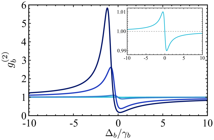
Figure 4: Second-order coherence function $g^{(2)}_{b}$ of an anharmonic oscillator, as a function of the detuning $\Delta_{b}$ From light to dark blue, $U$ increases (the exact values are $U/\gamma_{b}=0.01,\,0.1,\,1,\,2$, for fixed $\gamma_{b}=1$). A zoom-in of the smallest case is shown in the inset.

To show that the effects of conventional (self-homodyne interference at all $N$) and unconventional (self-homodyne interference at a given $N$ only) blockades take place in a general setting and are not specific of strong quantum nonlinearities (such as a 2LS), we now address the case of a single anharmonic oscillator, that describes an interacting bosonic mode with a Kerr-type nonlinearity, which can be very weak. With driving by a coherent source (a laser) at frequency $\omega_{\mathrm{L}}$, its Hamiltonian reads

$$H_{\mathrm{ao}}=\Delta_{b}\,{b^{\dagger}}b+\frac{U}{2}\,{b^{\dagger}}{b^{\dagger}}bb+\Omega_{b}({b^{\dagger}}+b),$$ (29)

where the cavity operators are represented by ${b^{\dagger}}$ and $b$, $\Delta_{b}=\omega_{b}-\omega_{\mathrm{L}}$ is the detuning between the cavity and the laser, $U$ denotes the particle interaction strength (that provices the nonlinearity) and the driving amplitude is given by $\Omega_{b}$. This is the particular case of the general Hamiltonian (1) when only one mode is considered and $U$ remains finite and, generally, small. The level structure of this system (at vanishing driving) is given by the simple expression $E^{(N)}=N\omega_{b}+N(N-1)U$. The condition for the laser frequency to hit resonantly the $N$-photon level is $\omega_{\mathrm{L}}=E^{(N)}/N$ (or $\Delta_{b}=-(N-1)U/2$).

We restrict our analysis of the dynamics $\dot{\rho}=-i\,[H_{\mathrm{ao}},\rho]+(\gamma_{b}/2)\mathcal{L}_{b}\rho$, with $\gamma_{b}$ the decay rate of the mode, to the case of vanishing pumping, i.e. $\Omega_{b}\ll\gamma_{b}$. Solving the correlator equations in this limit gives the population

$$\langle n_{b}\rangle=\frac{\Omega_{b}^{2}}{\gamma_{b}^{2}+4\Delta_{b}^{2}}\,,$$ (30)

the 2nd-order Glauber correlator

$$g^{(2)}_{b}=\frac{\langle{b^{\dagger}}{b^{\dagger}}bb\rangle}{\langle{b^{\dagger}}b\rangle^{2}}=\frac{\big{(}\gamma_{a}^{2}+4\Delta_{b}^{2}\big{)}}{\gamma_{b}^{2}+(U+2\Delta_{b})^{2}}\,,$$ (31)

as well as the higher-order correlators

$$g^{(N)}_{b}=\frac{\big{(}\gamma_{a}^{2}+4\Delta_{b}^{2}\big{)}^{n-1}}{\prod_{k=1}^{n-1}\big{[}\gamma_{b}^{2}+\big{(}kU+2\Delta_{b}\big{)}^{2}\big{]}}\,.$$ (32)

This shows that, when scanning in frequency, $g^{(2)}_{b}$ has two extrema, one minimum and one maximum, as can be seen in Fig. 4, whose positions are given by

$$\Delta_{\pm}=-\frac{1}{4}\Big{(}U\pm\sqrt{U^{2}+4\gamma_{b}^{2}}\,\Big{)},$$ (33)

with respective optimum antibunching ($-$) and bunching $(+)$

$$g^{(2)}_{b}\big{(}\Delta_{b}=\Delta_{\pm}\big{)}=1+\frac{U\Big{(}U\pm\sqrt{U^{2}+4\gamma_{b}^{2}}\Big{)}}{2\gamma_{b}^{2}}.$$ (34)

Both of these features are linked to the level structure: the antibunching condition is that of resonantly driving the first rung, $E^{(1)}$ (note that $\Delta_{-}\sim 0$, especially when $U\gg\gamma_{b}$), and the bunching condition, that of driving the second rung, $E^{(2)}$ ($\Delta_{+}\sim-U/2$). In both cases, all other rungs are off-resonance and will remain much less occupied. Therefore, these effects are of a conventional nature, as we have defined it in the previous section: CA and conventional bunching (CB), respectively. The difference with resonance fluorescence is that here, CA is not a perfect interference at all orders ($g^{(N)}=0$ for $N>1$) but an approximated one. For instance, $g^{(2)}\approx(\gamma_{b}/U)^{2}$ (to leading order in $U/\gamma_{b}$), is only zero in the limit $U\rightarrow\infty$, when the system converges to a 2LS. On the other hand, there was not CB in resonance fluorescence due to the lack of levels $N>1$. Here, we see it appearing for the first time.

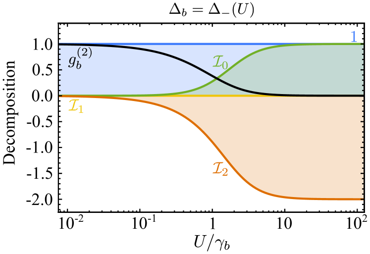
Figure 5: Second-order coherence function $g^{(2)}_{b}$ together with its decomposition, as a function of the non-linear interactionnonlinearity strength $U$ following the conventional antibunching frequency $\Delta_{b}=\Delta_{-}(U)$.

The decomposition $g^{(2)}_{b}$ of according to Eq. (6) yields

$$\mathcal{I}_{0}= \,\frac{U^{2}}{\gamma_{b}^{2}+(U+2\Delta_{b})^{2}}\,,$$ (35a)

$$\mathcal{I}_{1}= \,0\,,$$ (35b)

$$\mathcal{I}_{2}= \,-\frac{2U\big{(}U+2\Delta_{b}\big{)}}{\gamma_{b}^{2}+(U+2\Delta_{b})^{2}}\,.$$ (35c)

$\mathcal{I}_{0}>0$ means that fluctuations are always super-poissonian. $\mathcal{I}_{1}$ vanishes in the limit of low driving (as in the case of the Heitler regime), which means that there are no anomalous correlations to leading order in $\Omega_{b}$. The remaining term $\mathcal{I}_{2}$ can take positive (for $\Delta_{b}>-U/2$) and negative (for $\Delta_{b}<-U/2$) values, resulting in super-Poissonian statistics or on the contrary favouring antibunching. The various terms and the total $g^{(2)}_{b}$ are shown in Fig. 5 as a function of $U$, for the case $\Delta_{b}=\Delta_{-}(U)$ that maximizes antibunching, showing the evolution from Poissonian fluctuations in the linear regime of a driven harmonic mode to antibunching as the two-level limit is recovered with $\mathcal{I}_{0}\rightarrow 1$ and $\mathcal{I}_{2}\rightarrow-2$ (cf. Fig. 2(a)).

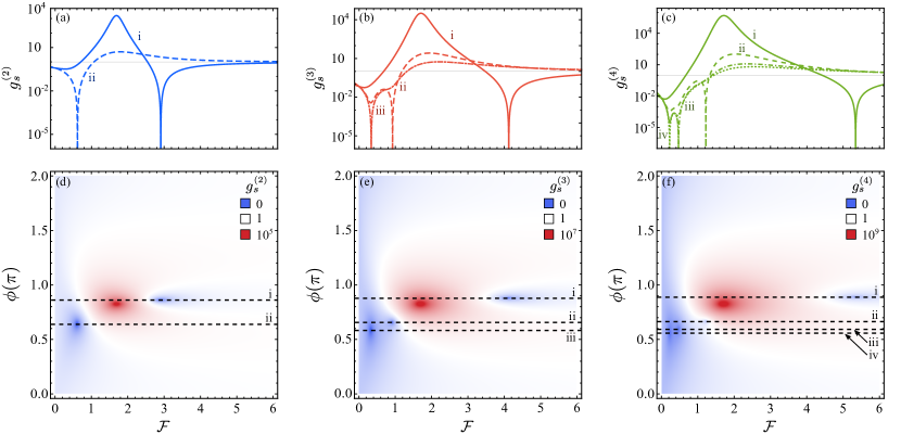
Figure 6: (Color online) Interference between the output of a driven anharmonic system and an external laser of intensity proportional to $\mathcal{F}$ and phase $\phi$. Various columns shown increasing orders of photon correlations, with the upper row showing a phase-cut along the lines that intercept one of the resonances in the full landscape shown in the bottow row (the superbunching case is not shown). Parameters: $U=\gamma_{b}$, $\Omega_{b}=0.001\,\gamma_{b}$, $\mathrm{T}=0.5$ and $\gamma_{b}=1$.

As previously, the statistics can be modified by adjusting the coherent component of the original signal $b$ with an external laser $\beta=|\beta|e^{i\phi}$. The resulting signal is then described by the operator $s=\mathrm{T}b+i\,\mathrm{R}\beta$, with coherent contribution now given by $\langle s\rangle=\mathrm{T}\langle b\rangle+i\,\mathrm{R}\beta$. To simplify further the calculations, we choose $\beta=\frac{\mathrm{T}}{\mathrm{R}}\beta^{\prime}$, where $\beta^{\prime}$ is also written in terms of the driving amplitude and an adimensional amplitude $\mathcal{F}$:

$$\beta^{\prime}=\frac{\Omega_{b}}{\gamma_{b}}\mathcal{F}\,.$$ (36)

Additionally, we shift the phase $\phi\rightarrow\phi+\pi$ so in the limit of high $U$, all the results are consistent with the previous case. Then, the total population becomes:

$$\langle n_{s}\rangle=\frac{\mathrm{T}^{2}\Omega_{b}^{2}}{\gamma_{b}^{2}\big{(}\gamma_{b}^{2}+4\Delta_{b}^{2}\big{)}}\big{[}\mathcal{F}^{2}\big{(}\gamma_{b}^{2}+4\Delta_{b}^{2}\big{)}+4\gamma_{b}\mathcal{F}\big{(}\gamma_{b}\cos\phi-2\Delta_{b}\sin\phi\big{)}+4\gamma_{b}^{2}\big{]}\,,$$ (37)

and the 2-photon correlations become

$$\begin{split}g^{(2)}_{s}=&\tilde{\Gamma}_{b}^{2}\Big{\{}\tilde{\Gamma}_{b}^{2}\big{[}\gamma_{b}^{2}+(U+\Delta_{b})^{2}\big{]}\mathcal{F}^{4}+8\gamma_{b}\big{[}\gamma_{b}^{2}+(U+\Delta_{b})^{2}\big{]}(\gamma_{b}\cos\phi-2\Delta_{b}\sin\phi)\mathcal{F}^{3}+\big{[}16\gamma_{b}^{2}\big{(}\gamma_{b}^{2}+(U+2\Delta_{b})^{2}\big{)}+\\ &8\gamma_{b}^{2}\cos 2\phi\,\big{(}\gamma_{b}^{2}-2\Delta_{b}(U+2\Delta_{b})\big{)}-8\gamma_{b}^{3}\sin 2\phi(U+4\Delta_{b})\big{]}\mathcal{F}^{2}+32\gamma_{b}^{3}\big{[}\gamma_{b}\cos\phi-(U+2\Delta_{b})\sin\phi\big{]}\mathcal{F}+16\gamma_{b}^{2}\Big{\}}\biggm{/}\\ &\Big{\{}\big{[}\gamma_{b}^{2}+(U+2\Delta_{b})^{2}\big{]}\big{[}\mathcal{F}^{2}\big{(}\gamma_{b}^{2}+4\Delta_{b}^{2}\big{)}+4\gamma_{b}\mathcal{F}\big{(}\gamma_{b}\cos\phi-2\Delta_{b}\sin\phi\big{)}+4\gamma_{b}^{2}\big{]}^{2}\Big{\}},\end{split}$$ (38)

where we have used $\tilde{\Gamma}_{b}^{2}=\gamma_{b}^{2}+4\Delta_{b}^{2}$. Here as well, we can compare the enrichment brought by the interfering laser by comparing Eqs. (30) and (37) for populations and Eqs. (31) and (38) for second-order correlations, with and without the interference, respectively. In this case, higher-order correlators could also be given in closed-form but is too awkward to be written here. The cases $g_{s}^{(k)}$ for $2\leq k\leq 4$ are shown in Fig. 6 as a function of the parameters of the interfering laser. By comparing this to Fig. 3 for the 2LS, one can see that the anharmonic system is significantly more complex, with resonances for the correlations that occur for specific conditions of the phase for each $\mathcal{F}$ that leads to unconventional forms of antibunching or superbunching, rather than to be simply out-of-phase previously. This makes salient the punctual character of the unconventional mechanism: each strong correlation at any given order must be realized in a very particular way: the one that matches the corresponding interference.

The maximum bunching (UB) accessible with the interfering laser is reached when the coherent-fraction population goes to zero (1-photon suppression) for which the conditions on the phase and amplitude read

$$\tan\phi_{1}=-\frac{2\Delta_{b}}{\gamma_{b}}\quad\quad\mathrm{and}\quad\quad\mathcal{F}_{1}=-2\cos\phi_{1}\,.$$ (39)

Those conditions are exactly the same as Eq. (27) for $N=1$. Analogous conditions for the multi-photon cases can be found solving $g^{(N)}_{s}=0$. For the case $N=2$, we find four different roots:

$$\mathcal{F}_{2,1/2}= \frac{2ie^{i\phi}\gamma_{b}}{(U+2\Delta_{b})+i\gamma_{b}}\bigg{\{}1\pm\sqrt{\frac{U}{(U+2\Delta_{b})+i\gamma_{b}}}\bigg{\}}\,,$$ (40a)

$$\mathcal{F}_{2,3/4}= \frac{2ie^{-i\phi}\gamma_{b}}{(U+2\Delta_{b})-i\gamma_{b}}\bigg{\{}1\pm\sqrt{\frac{U}{(U+2\Delta_{b})-i\gamma_{b}}}\bigg{\}}^{-1}\,.$$ (40b)

Since these should be, by definition, real, this imposes another constrain on $\phi$. Although the expression for real-valued $\phi$ to make $\mathcal{F}$ real cannot be given in closed form, they are readily found numerically. It is possible to get four real solutions, that are however degenerate. There are only two different conditions for $\phi$ since the real part is the same for each pair of roots, i.e., $\real(\mathcal{F}_{2,1})=\real(\mathcal{F}_{2,4})$ and $\real(\mathcal{F}_{2,2})=\real(\mathcal{F}_{2,3}))$. This yields two physical solutions. For instance, for $U=\gamma_{b}$ and $\Delta_{b}=\Delta_{-}$ (the case shown in Fig. 6), $g^{(2)}_{s}$ vanishes at $\mathcal{F}_{2,1}\approx 0.615$ and $\mathcal{\phi}_{2,1}\approx 0.659\,\pi$ for one solution and at $\mathcal{F}_{2,2}\approx 2.907$ and $\mathcal{\phi}_{2,2}\approx 0.860\,\pi$ for the other one. Similar resonances in higher-order correlations could be found following the same procedure.

Regarding the quantum state realized in the system, similar conclusions can be drawn for the anharmonic oscillator than for the two-level system (previous Section, cf. Tables 1 and 2). Specifically for this case, the system can be described by a displaced squeezed thermal state, properly parameterized, but to lowest-order in the driving and for the population and the two-photon correlation only. Departures arise to next-order in the pumping or to any-order for three-photon correlations and higher. The main differences is that the anharmonic oscillator case has to be worked out numerically, so the prefactors are given by the solutions that optimize the antibunching, for the system parameters indicated in the caption. The same result otherwise holds that the Gaussian-state description is a low-driving approximation valid for the population and two-photon statistics. The same holds for the systems studied in the following Sections, although this point will not be stressed anymore.

VI Jaynes–Cummings blockade

Now that we have considered the two-level system on the one hand (Section IV) and the bosonic mode on the other hand (Section V), we turn to the richer and intricate Physics that arises from their coupling. We will show how the themes of the previous Sections allow us to unify in a fairly concise picture the great variety of phenomena observed and/or reported in isolation.

We thus consider the case where a cavity mode, with bosonic annihilation operator $a$ and frequency $\omega_{a}$, is coupled to a 2LS, with operator $\sigma$ and frequency $\omega_{\sigma}$, with a strength given by $g$. Such a system is described by the Jaynes–Cummings Hamiltonian jaynes63a ; shore93a ,

$$H_{\mathrm{jc}}=\Delta_{\sigma}{\sigma^{\dagger}}\sigma+\Delta_{a}{a^{\dagger}}a+g\left({a^{\dagger}}\sigma+{\sigma^{\dagger}}a\right)+{}\\ {}+\Omega_{a}\left(e^{i\phi}{a^{\dagger}}+e^{-i\phi}a\right)+\Omega_{\sigma}\left({\sigma^{\dagger}}+\sigma\right),$$ (41)

where we also include both a cavity and a 2LS driving term by a laser of frequency $\omega_{\mathrm{L}}$, with respective intensities $\Omega_{a}$ and $\Omega_{\sigma}$ and relative phase $\phi$. We assume $g$ and $\Omega_{\sigma}$ to be real numbers, without loss of generality since the magnitudes of interest ($G_{a}^{(N)}$) are independent of their phases. The relative phase $\phi$ between dot and cavity drivings is, on the other hand, important. We also limit ourselves in this text to the case where the frequencies of the dot and cavity drivings $\omega_{\mathrm{L}}$ are identical and the analysis could be pushed further to the case where this limitation is lifted. The dissipation is taken into account through the master equation $\partial_{t}\rho=i\left[\rho,H_{\mathrm{jc}}\right]+(\gamma_{\sigma}/2)\mathcal{L}_{\sigma}\rho+(\gamma_{a}/2)\mathcal{L}_{a}\rho$ where $\gamma_{a}$ is the decay rate of the cavity. We solve the steady state in the low-driving regime, i.e., when $\Omega_{a}\ll\gamma_{a}\,,\gamma_{\sigma}$, as indicated in Appendix D and find the populations:

$$\langle n_{\begin{subarray}{c}a\\ \sigma\end{subarray}}\rangle=4\,\frac{4g^{2}\Omega_{\begin{subarray}{c}a\\ \sigma\end{subarray}}^{2}+\tilde{\Gamma}_{\begin{subarray}{c}\sigma\\ a\end{subarray}}^{2}\Omega_{\begin{subarray}{c}a\\ \sigma\end{subarray}}^{2}-4g\Omega_{a}\Omega_{\sigma}\left(\pm 2\Delta_{\begin{subarray}{c}a\\ \sigma\end{subarray}}\cos\phi+\gamma_{\begin{subarray}{c}\sigma\\ a\end{subarray}}\sin\phi\right)}{16g^{4}+8g^{2}\left(\gamma_{a}\gamma_{\sigma}-4\Delta_{a}\Delta_{\sigma}\right)+\tilde{\Gamma}_{a}^{2}\tilde{\Gamma}_{\sigma}^{2}}\,,$$ (42)

with matching upper/lower indices (including $\pm$) and with $\tilde{\Gamma}^{2}_{i}=\gamma_{i}^{2}+4\Delta_{i}^{2}$ (for $i=a,\sigma$). Similarly, we find the two-photon coherence function from the cavity:

$$\begin{split}g^{(2)}_{a}=&\Big{\{}\Big{[}16g^{4}+8g^{2}\left(\gamma_{a}\gamma_{\sigma}-4\Delta_{a}\Delta_{\sigma}\right)+\tilde{\Gamma}_{a}^{2}\tilde{\Gamma}^{2}_{\sigma}\Big{]}\Big{[}16g^{4}\left(1+\chi^{2}\right)+8g^{2}\big{(}2\chi^{2}\tilde{\Gamma}_{11}^{2}+4\Delta_{\sigma}\tilde{\Delta}_{11}-\gamma_{\sigma}\tilde{\gamma}_{11}\big{)}+\tilde{\Gamma}^{2}_{\sigma}\tilde{\Gamma}_{11}^{2}-\\ &16g\chi\big{(}\Delta_{\sigma}\tilde{\Gamma}_{11}^{2}+4g^{2}\tilde{\Delta}_{11}[1+\chi^{2}]\big{)}\cos\phi+8g^{2}\chi^{2}\big{(}4g^{2}-\gamma_{\sigma}\tilde{\gamma}_{11}+4\Delta_{\sigma}\tilde{\Delta}_{11}\big{)}\cos 2\phi\,-\\ &8g\chi\big{(}\gamma_{\sigma}\tilde{\Gamma}_{11}^{2}+4g^{2}\tilde{\gamma}_{11}[\chi^{2}-1]\big{)}\sin\phi+16g^{2}\chi^{2}\big{(}\gamma_{a}\Delta_{\sigma}+\gamma_{\sigma}\tilde{\Delta}_{12}\big{)}\sin 2\phi\Big{]}\Big{\}}\Big{/}\\ &\Big{\{}\Big{[}16g^{4}+8g^{2}\Big{(}\gamma_{a}\tilde{\gamma}_{11}-4\Delta_{a}\tilde{\Delta}_{11}\Big{)}+\tilde{\Gamma}_{a}^{2}\tilde{\Gamma}_{11}^{2}\Big{]}\Big{[}4g^{2}\chi^{2}+\tilde{\Gamma}_{\sigma}^{2}-4g\chi\big{(}2\Delta_{\sigma}\cos\phi+\gamma_{\sigma}\sin\phi\big{)}\Big{]}^{2}\Big{\}},\end{split}$$ (43)

where $\tilde{\Delta}_{ij}\equiv i\Delta_{a}+j\Delta_{\sigma}$, $\tilde{\gamma}_{ij}=i\gamma_{a}+j\gamma_{\sigma}$, $\tilde{\Gamma}_{ij}^{2}\equiv\tilde{\gamma}_{ij}^{2}+4\tilde{\Delta}^{2}_{ij}$ and $\chi=\Omega_{\sigma}/\Omega_{a}$ is the ratio of excitation. The range of $\chi$ extends from 0 to $\infty$ so that it is convenient to use the derived quantity $\tilde{\chi}=\frac{2}{\pi}\atan(\chi)$ which varies between 0 and 1. Equation (43) is admittedly not enlightening per se but it contains all the physics of conventional and unconventional photon statistics that arises from self-homodyning, including bunching and antibunching, for all the regimes of operations. It is quite remarkable that so much physics of dressed-state blockades and interferences can be packed-up so concisely.

We plot a particular case of this formula as a function of $\omega_{a}$ and $\omega_{\mathrm{L}}$ in Fig. 7(a), namely, only driving the cavity ($\Omega_{\sigma}=\chi=0$). Its reduced expression, Eq. (65), is given in Appendix I. The general case is available through an applet wolfram_casalengua18a and we will shortly discuss other cases as well. The structure that is thus revealed can be decomposed in two classes, as shown in panel (b): the conventional statistics that originates from the nonlinear properties of the quantum levels, in solid lines, and the unconventional statistics that originates from interferences, in dashed lines. Both can give rise to bunching (in red) and antibunching (in blue). We now discuss them in details.

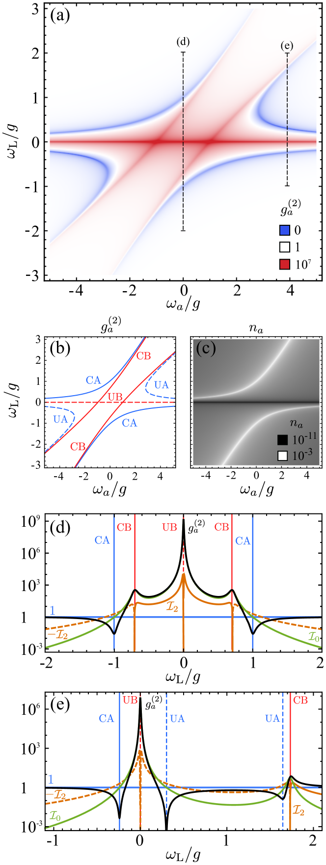
Figure 7: (Color online) Jaynes–Cummings model. (a) Photon statistics $g^{(2)}_{a}$ (log scale). (b) Structure in terms of conventional C (solid) and unconventional U (dashed) features for B, bunching (blue) and A, antibunching (red). CA (CB) is given by the resonant condition with the first (second) JC rung, cf. Eqs. (44). UA is given by the interference condition Eq. (45) and UB by $\omega_{\mathrm{L}}=0$. (c) Population $n_{a}$, showing that i) only polariton emit strongly and ii) how the depletion (not an exact zero) at $\omega_{\mathrm{L}}=0$ accounts for UB. Other features are not visible in the population only. (d-e) $g^{(2)}_{a}$ (black line) for the two cuts shown in dashed lines in (a) with the cavity frequency either (d) resonant with the 2LS or (e) chosen to optimise UA ($\omega_{a}=29.5\gamma_{\sigma}$). The decomposition in $\mathcal{I}_{j}$ components (from Appendix G) is also shown, with the sign of $\mathcal{I}_{2}$ changed when it is negative and plotted dashed. Parameters: $\omega_{\sigma}=0$, $\gamma_{a}=0.1\,g$ and $\gamma_{\sigma}=0.01\,g$.

VI.1 Conventional statistics

Conventional features arise from the laser entering in resonance with a dressed state of the dissipative JC ladder delvalle09a ; laussy12e , which energy is the real part of

$$E^{(N)}_{\pm}=N\omega_{a}+\frac{\omega_{\sigma}-\omega_{a}}{2}-i\frac{(2N-1)\gamma_{a}+\gamma_{\sigma}}{4}\\ \pm\sqrt{(\sqrt{N}g)^{2}+\left(\frac{\omega_{a}-\omega_{\sigma}}{2}-i\frac{\gamma_{a}-\gamma_{\sigma}}{4}\right)^{2}}\,.$$ (44)

The first rung $E^{(1)}_{\pm}$ yields the CA lines in Fig. 7(b). This corresponds to an increase in the cavity population, as shown in Fig. 7(c) as two white lines, corresponding to the familiar lower and upper branches of strong coupling. The system effectively gets excited, but through its first rung only. The second rung blocks further excitation according to the conventional antibunching (CA), or photon-blockade, scenario, so that with the increase of population goes a decrease of two-photon excitation, leading to antibunching. This is in complete analogy with the CA that appears in the Heitler regime of resonance fluorescence. This is not an exact zero in $g^{(2)}_{a}$ in the low driving regime (the imaginary part of the root does not vanish) because the conditions for perfect interference are no longer met having a strongly coupled cavity with a decay rate. We recently showed in Ref. lopezcarreno18b that even in the vanishing coupling regime, $g\rightarrow 0$, when the cavity acts as a mere detector of the 2LS emission, perfect antibunching is spoiled due to the finite decay rate ($\gamma_{a}$ representing the precision in frequency detection). This is due to the fact that the cavity is effectively filtering out some of the incoherent fraction of the emission while the coherent fraction is still fully collected. The interference condition in the $g^{(2)}_{a}$ decomposition, $1+\mathcal{I}_{1}=-\mathcal{I}_{2}=2$, is no longer satisfied (see Fig. 2 of Ref. lopezcarreno18b ).

On the other hand, driving resonantly the second rung, $E^{(2)}_{\pm}$, leads to conventional bunching (CB), shown as red solid lines in Fig. 7(b). These quantum features are well known and also found with incoherent driving of the system in the spectrum of emission laussy12e , they are not conditional to the coherence of the driving. This also corresponds to an increase in the cavity population although this is not showing in Fig. 7(c), where only first order effects appear.

VI.2 Unconventional statistics

We now turn to the other features in $g^{(2)}_{a}$ that do not correspond to a resonant condition with a dressed state: these are, first, a superbunching line at $\omega_{\mathrm{L}}=0$ (dashed red in Fig. 7(b)) and second, two symmetric antibunched lines (dashed blue). All correspond to a self-homodyne interference that the coherent field driving the cavity can produce on its own, without the need of a second external laser. In this case, this also involves several modes (degrees of freedom) and more parameters than in resonance fluorescence, so the phenomenology is richer, but can be tracked down to the same physics. We call them again unconventional antibunching (UA) and unconventional bunching (UB) in full analogy with the Heitler regime of resonance fluorescence and in agreement with the literature that refers to particular cases of this phenomenology as “unconventional blockade” bamba11a (the term of “tunnelling” has also been employed but the underlying physical picture might be misleading faraon08a ).

We first address antibunching (UA). This is found by minimizing $g^{(2)}_{a}$ in regions where there is no CA, which yields (for the particular case $\chi=0$):

$$\Delta_{a}=-\Delta_{\sigma}\left(1+\frac{4g^{2}}{\gamma_{\sigma}^{2}+4\Delta_{\sigma}^{2}}\right)\,,$$ (45)

which is the analytical expression for the the dashed blue lines in Fig. 7(b) (we remind that $\Delta_{i}\equiv\omega_{i}-\omega_{\mathrm{L}}$ for $i=a$, $\sigma$). The most general case when both the emitter and cavity are excited is given in Appendix H. In the minimization process, we also find the condition for CA, due to the first-rung resonance, but this can be disconnected from UA beyond the fact that CA is already identified, because of UA also admits an exact zero, which is found by either solving $g^{(2)}_{a}=0$ or setting to zero the two-photon probability in the wavefunction approximation visser95a (see Appendix F.2). This gives the conditions on the detunings as function of the system parameters :

$$\Delta_{\sigma}^{2} =\frac{\gamma_{\sigma}^{2}}{4}\left(\frac{4g^{2}}{\gamma_{\sigma}(\gamma_{\sigma}+\gamma_{a})}-1\right)\,,$$ (46a)

$$\Delta_{a} =-\bigg{(}2+\frac{\gamma_{a}}{\gamma_{\sigma}}\bigg{)}\Delta_{\sigma}\,.$$ (46b)

These conditions are met in Fig. 7(a) at the lowest point where the blue UA line intersects the (e) cut (and on the symmetric point $\omega_{a}<0$). When the laser is at resonance with the 2LS ($\Delta_{\sigma}=0$) and cavity losses are large ($\gamma_{a}\gg\gamma_{\sigma}$), this occurs when the cooperativity $\mathscr{C}\equiv\frac{4g^{2}}{\gamma_{a}\gamma_{\sigma}}=1$. This type of UA interference is second-order, so it is not apparent in the cavity population at low driving, Fig. 7(b). One has to turn to two-photon correlations instead. Note also that UA requires a cavity-emitter detuning that is of the order of $g$.

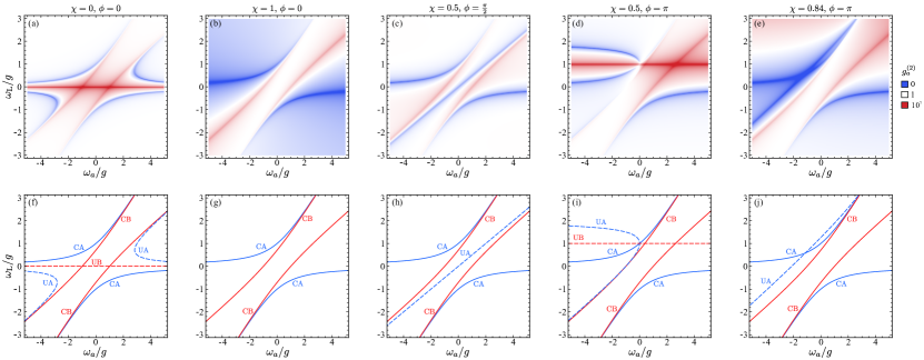
Figure 8: (Color online) Effect of the type of driving on the two-photon statistics, for the Jaynes–Cumming model as measured in its cavity emission. The upper row shows Eq. (43) for the parameters indicated in each panel and the lower row identifies the various features through the structure of conventional (Eq. (44c), solid) and unconventional (Eq. (45), dashed) lines. Chosen parameters: $\gamma_{a}=0.1\,g$, $\gamma_{\sigma}=0.01\,g$.

Since this is an interference effect, we perform the same decomposition of $g^{(2)}_{a}$ in terms of coherent and incoherent fractions, as in previous Sections, given by Eq. (6), and show the terms that are not zero in Fig. 7(d-e). The full expressions are in Appendix G. The term $\mathcal{I}_{1}$ is exactly zero to lowest order in the driving and only the fluctuation-statistics $\mathcal{I}_{0}$ and the two-photon interference $\mathcal{I}_{2}$ play a role, like in the Heitler regime of resonance fluorescence. We observe that, in this decomposition, there is no difference between the CA and UA, since both occur approximately when the statistics of the laser and fluctuations, $1+\mathcal{I}_{0}=2$, are compensated by their two-photon interference, $\mathcal{I}_{2}=-2$, again as in the Heitler regime. The fundamental differences between these two types of antibunching will be discussed later on. Before that, we discuss the last feature: the unconventional bunching at $\omega_{\mathrm{L}}=0$.

The reason for the super-bunching peak labelled as UB in Fig. 7(b) is also the same as in resonance fluorescence: the cancellation of the coherent part, in this case, of the cavity emission, and the consequent dominance of the fluctuations only, which are super-Poissonian in this region. Therefore, contrary to the CB, this superbunched statistics is not directly linked to an enhanced $N$-photon (for any $N$) emission and it does not appear one could harvest or Purcell-enhance it, for instance, by coupling the system to an auxiliary resonant cavity. Since it is pretty much wildly fluctuating noise, the actual prospects of multi-photon physics in this context remains to be investigated. In any case, the conditions that yield the super-Poissonian correlations can thus be obtained by minimising the cavity population $\langle n_{a}\rangle$ or, from the wavefunction approximation detailed in Appendix (F.2), by minimising the probability to have one photon, given by Eq. (50), which coincide with the coherent fraction to lowest order in $\Omega_{a}$. One cannot achieve an exact zero in this case but the cavity population is clearly undergoing a destructive interference, as shown by the black horizontal line in Fig. 7(c). The resulting condition links the laser frequency with the 2LS one:

$$\Delta_{\sigma}=\chi g\cos\phi\,,$$ (47)

which reduces to simply $\Delta_{\sigma}=0$ (laser in resonance with the 2LS) if i) the dot and cavity are driven with a $\pi/2$-phase difference or ii) the laser drives the cavity only ($\chi=0)$.

So far, we have focused on the particular case of Eq. (43) where $\Omega_{\sigma}=0$ (i.e., Eq. (65)). This is the case dominantly studied in the literature and the one assumed to best reflect the experimental situation. It is also for our purpose a good choice to clarify the phenomenology that is taking place and how various types of statistics cohabit. It must be emphasised, however, that while the physics is essentially the same in the more general configuration, the results are, even qualitatively, significantly different in configurations where the two types of pumping are present. This is shown in Fig. 8. While conventional features are stable, being pinned to the level structure, the unconventional ones that are due to interferences are very sensible to the excitation conditions and get displaced or, in the case of QD excitation only, even completely suppressed. If one is to regard conventional features as more desirable for applications, this figure is therefore again an exhortation at focusing on the QD excitation configuration.

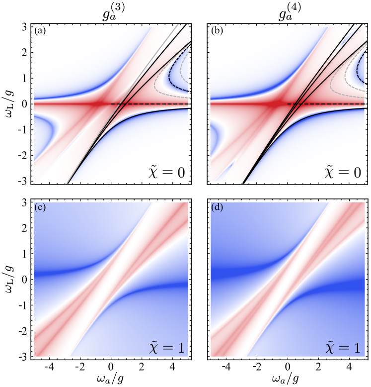
Figure 9: (Color online). Higher-order photon statistics, at (left column) three- and (right) four-photon level. Top row is for cavity excitation and bottom row for 2LS excitation. In the top row, we have superimposed the right-half of the conventional (solid) and unconventional (dashed) features, putting them in grey when not present for a given order of the correlations. The conventional features grow in numbers and stay pinned at the same positions while the unconventional ones remain in the same number but at different positions. Parameters: $\gamma_{a}=0.1\,g$, $\gamma_{\sigma}=0.001\,g$.

While we have focused on the two-photon statistics, both the conventional and unconventional effects occur at the $N$-photon level, in which case they manifest through higher-order coherence functions $g^{(N)}$, and their $N$th-order behaviour is one of the key differences between conventional and unconventional statistics. Regarding conventional features, resonances happen at the $N$-photon level when $N$ photons of the laser have the same energy than one of the dressed states (and only one, thanks to the JC nonlinearities): $\omega_{\mathrm{L}}=\mathrm{Re}\{E^{(N)}_{\pm}\}/N$. The blockade that is realised is a real blockade in the sense that all the correlation functions are then depleted simultaneously. In Fig. 9, the counterpart of Fig. 7(a) is shown for $g^{(3)}_{a}$ and $g^{(4)}_{a}$ and shows how more conventional features appear with increasing $N$ but otherwise stay pinned to the same conditions, while the number of unconventional features stays the same, but their positions drift with $N$, so that one cannot simultaneously realise $g^{(N)}_{a}<1$ for all $N$. This is an important difference between a convex mixture of Gaussian states, which is a semi-classical state, and a state beyond this class, which is genuinely quantum, as previously mentioned. The latter requires the ability to imprint strong correlations at several and possibly all photon-orders. This suggests that CA could be more suited than UA for quantum applications. Note how with the 2LS direct excitation, shown in the second row of Fig. 9, one only finds conventional statistics, with magnified features such as broader antibunching in the photon-like branch and narrower one in the exciton-like branch. The $N$-photon resonances are neatly separated for large-enough detuning, which is the underlying principle to harness rich $N$-photon resources sanchezmunoz14a .

Figure 10: (Color online) Transition to weak coupling and non-vanishing pumping. (a) Evolution of $g^{(2)}_{a}$ along the cut (e) in Fig. 7 as a function of the coupling strength $g$, showing how the structure collapses on the bare modes. CA (lowest blue line) is the first feature to vanish with decreasing $g$, as the underlying dressed states disappear. (b) Behaviour of the “center” point at $\omega_{\mathrm{L}}=\omega_{a}=0$, that typically features the UB peak, although not exclusively as it can also exhibit antibunching, even in strong-coupling (Black dashed line indicates when the behaviour of $g^{(2)}_{a}$ changes from local minimum to maximum). (c) Effect of increasing pumping, computing the features shown in Fig. 7(e) (vanishing pumping) as a function of (finite) driving $\Omega_{a}$. For high pumping, $\Omega_{a}\gtrsim\gamma_{a}$, every feature (both bunching and antibunching) is spoiled and eventually disappears ($g^{(2)}_{a}\rightarrow 1$). The inset figure compares the same cut of $g^{(2)}_{a}$ for the cases of vanishing driving ($\Omega_{a}\rightarrow 0$) and finite driving ($\Omega_{a}/\gamma_{a}=0.5,2\ \text{and}\ 10$). Lighter colors correpond to higher driving amplitudes.

We now turn to another noteworthy regime, out of the many configurations of interest that are covered by Eq. (43), namely, the transition from weak to strong coupling. The so-called strong-coupling, when $g>|\gamma_{a}-\gamma_{\sigma}|/4$, is one of the coveted attributes of light-matter interactions, leading to the emergence of dressed states and to a new realm of physics. It is also, however, an ill-defined concept in presence of detuning laussy12e and one would still find the dressed-state structure of Fig. 9 in the largely detuned regime when driving the 2LS, even up to large photon-order kavokin_book17a . The restructuration of the statistics when crossing over to the weak-coupling regime is explored in Fig. 10(a), where we track the impact on $g^{(2)}_{a}$ of changing the coupling $g$, on the cut in Fig. 7(e) that intersects from top to bottom CB, UA (twice), UB and CA. One can see how the features converge as the coupling is reduced, with the conventional ones disappearing first, which is expected from the disappearance of the underlying dressed states, that are responsible for the conventional effects. The unconventional antibunching, on the other hand, is more robust and can be tracked well into weak coupling where all effects ultimately vanish at the same time as they merge. Conventional antibunching is the most robust feature, as can be seen by tracking for instance the UB peak at the point where it is the most isolated from the other features, namely, at resonance where $\omega_{\mathrm{L}}=\omega_{a}=\omega_{\sigma}=0$. Spanning over the two main parameters that control strong coupling, the coupling strength $g$ (in units of $\gamma_{\sigma}$) and the rates of dissipation rates $\gamma_{a}/\gamma_{\sigma}$, one sees that the strong bunching is not always sustained but can be instead overtaken by conventional antibunching, which is the well-defined blue line in the figure (given by Eq. (45)). The region where the UB peak is well-defined can be identified by inspecting the second derivative of $g^{(2)}_{a}$ as a function of the laser frequency, $\partial^{2}_{\omega_{\mathrm{L}}}g^{(2)}_{a}$ at $\omega_{\mathrm{L}}=0$ and is shown in Fig. 10(b) as a dashed black line. The white line that separates the antibunching region from the bunching one corresponds to the critical coupling strength $g_{P}$ between the cavity and the 2LS that leads to $g^{(2)}_{a}=1$ (its expression is given in the Appendix, Eq. (67)). The strong-weak coupling frontier $g/\gamma_{\sigma}<|\gamma_{a}/\gamma_{\sigma}-1|/4$ is indicated with a dotted green line as a reference, illustrating again the lack of close connection between strong-coupling and the photon-statistics features.

We conclude our discussion of the Jaynes-Cummings system with the second main difference between conventional and unconventional statistics, namely their resilience to higher driving. All our results are exact in the limit of vanishing driving, that is to say, in the approximation of neglecting $\Omega$ terms of higher-orders than the smallest contributing one. For non-vanishing driving, numerically exact results can be obtained instead (and can be made to agree with arbitrary precision to the analytical expressions, as long as the driving is taken low enough, what we have consistently checked). A characteristic of the unconventional features is that, being due to an interference effect for a given photon number only, it is fragile to driving, unlike the conventional features which display more robustness. This is illustrated in Fig. 10(c) for the case of cavity driving $\Omega_{a}$, where we compare the analytical result from Eq. (43) or, in this case, Eq. (65), in black, with the numerical solution for $\Omega_{a}=0.25\gamma_{a}$, so still fairly small. One can see how the conventional features are qualitatively preserved and quantitatively similar to the analytical result, while the unconventional antibunching has been completely washed out.

One could consider still other aspects of the Physics embedded in Eq. (43). We invite the inquisitive and/or interested readers to explore them through the applet wolfram_casalengua18a which is helpful to get a sense of the complexity of the problem. Instead of discussing these further, we now turn to another platform of interest that bears many similarities with the Jaynes–Cummings results.

VII Microcavity-polariton blockade

Microcavity polaritons kavokin_book17a arise from the strong coupling between a planar cavity photon and a quantum well exciton, both of which are bosonic fields with annihilation operators $a$ and $b$, respectively. These fields are coupled with strength $g$ and have frequencies $\omega_{a}$ and $\omega_{b}$. Moreover, the excitons, being electron-hole pairs, have Coulomb interactions that we parametrise as $U/2$. Thus, the Hamiltonian describing the polariton system is given by

$$H_{\mathrm{pol}}=\Delta_{a}{a^{\dagger}}a+\Delta_{b}{b^{\dagger}}b+g\left({a^{\dagger}}b+{b^{\dagger}}a\right)+{}\\ {}\Omega_{a}\left(e^{i\phi}{a^{\dagger}}+e^{-i\phi}a\right)+\Omega_{b}({b^{\dagger}}+b)+\frac{U}{2}{b^{\dagger}}{b^{\dagger}}bb\,,$$ (48)

where $\Delta_{a,b}=\omega_{a,b}-\omega_{\mathrm{L}}$ are the frequencies of cavity/exciton referred to $\omega_{\mathrm{L}}$, which is the frequency of the laser that drives the photonic/excitonic field with amplitudes $\Omega_{a,b}$. The phase difference between them is represented by $\phi=\phi_{a}-\phi_{b}$ and since the absolute phase can be chosen freely, $\phi_{a,b}$ are fixed to be $\phi$ and $0$. The dissipative dynamics of the polaritons is given by a master equation $\partial_{t}\rho=i\left[\rho,H_{\mathrm{pol}}\right]+(\gamma_{b}/2)\mathcal{L}_{b}\rho+(\gamma_{a}/2)\mathcal{L}_{a}\rho$, where $\gamma_{a}$ and $\gamma_{b}$ are the decay rates of the photon and the exciton, respectively. As compared to the Jaynes–Cummings Hamiltonian (41), the polariton Hamiltonian substitutes the 2LS by a weakly interacting Bosonic mode, $b\rightarrow\sigma$ with nonlinearities ${b^{\dagger}}{b^{\dagger}}bb$ thus slightly displacing the state with two excitations while the 2LS forbids it entirely. In the case where $U\rightarrow\infty$, the Jaynes–Cummings limit is recovered, but in most experimental cases, $U/\gamma_{a}$ is very small. In all cases, in the low driving regime ($\Omega_{a}\rightarrow 0$) the steady-state populations of the photon and the exciton are given by the same expressions as in the Jaynes–Cummings model, Eq. (42) with $\sigma\rightarrow b$, since the 2LS converges to a bosonic field in the linear regime. The differences arise in the two-particle magnitudes (cf. Eq. (43)):

$$\begin{split}g^{(2)}_{a}=&\Big{\{}\Big{[}16g^{4}+8g^{2}\big{(}\gamma_{a}\gamma_{b}-4\Delta_{a}\Delta_{b}\big{)}+\tilde{\Gamma}_{a}^{2}\tilde{\Gamma}_{b}^{2}\Big{]}\Big{[}\tilde{\Gamma}_{b}^{2}\tilde{\Gamma}_{11}^{2}\big{(}\gamma_{b}^{2}+\tilde{U}_{12}^{2}\big{)}+8g^{2}\Big{(}U^{2}[4\Delta_{b}\tilde{\Delta}_{11}-\gamma_{b}\tilde{\gamma}_{11}]+2\tilde{\Gamma}_{11}^{2}[\gamma_{b}^{2}+\tilde{U}_{12}^{2}]\chi^{2}+\\ &8U\Delta_{b}^{2}\tilde{\Delta}_{11}-2U\gamma_{b}^{2}\tilde{\Delta}_{13}-4U\gamma_{a}\gamma_{b}\Delta_{b}\Big{)}+16g^{4}\Big{(}U^{2}+[\tilde{\gamma}_{11}^{2}+(U+2\tilde{\Delta}_{11})^{2}]\chi^{4}\Big{)}-16g\chi\cos\phi\,\Big{(}\Delta_{b}\tilde{\Gamma}_{11}^{2}[\gamma_{b}^{2}+4\tilde{U}_{12}^{2}]\\ &+2g^{2}[U(2\tilde{\Delta}_{11}\tilde{U}_{12}-\gamma_{b}\tilde{\gamma}_{11})+(2U^{2}\tilde{\Delta}_{11}+2\Delta_{b}\tilde{\Gamma}_{11}^{2}+U\{\gamma_{a}\tilde{\gamma}_{11}+4\tilde{\Delta}_{11}\tilde{\Delta}_{12}\})\chi^{2}]\Big{)}+8g^{2}\chi^{2}\cos 2\phi\,\Big{(}4g^{2}U[U+2\tilde{\Delta}_{11}]-\\ &U^{2}[\gamma_{b}\tilde{\gamma}_{11}-4\Delta_{b}\tilde{\Delta}_{11}]-[\gamma_{b}^{2}-4\Delta_{b}^{2}]\tilde{\Gamma}_{11}^{2}+2U[\gamma_{a}^{2}\Delta_{b}+\tilde{\Delta}_{12}(4\Delta_{b}\tilde{\Delta}_{11}-\gamma_{b}^{2})]\Big{)}-8g\chi\sin\phi\,\Big{(}\gamma_{b}\tilde{\Gamma}_{11}^{2}[\gamma_{b}^{2}+\tilde{U}_{12}^{2}]+\\ &4g^{2}[\gamma_{b}\tilde{\Gamma}_{11}^{2}\chi^{2}+U(\chi^{2}-1)(U\tilde{\gamma}_{11}+2\gamma_{b}\Delta_{a}+2\tilde{\gamma}_{12}\Delta_{b})]\Big{)}+8g^{2}\chi^{2}\sin 2\phi\,\Big{(}-4g^{2}U\tilde{\gamma}_{11}+4\gamma_{b}\Delta_{b}\tilde{\Gamma}_{11}^{2}+2U^{2}[\gamma_{a}\Delta_{b}+\gamma_{b}\tilde{\Delta}_{12}]+\\ &U[\gamma_{a}^{2}\gamma_{b}+4\gamma_{b}\tilde{\Delta}_{12}^{2}+\gamma_{a}\tilde{\Gamma}_{b}^{2}]\Big{)}\Big{]}\Big{\}}\Big{/}\\ &\Big{\{}\Big{(}\tilde{\Gamma}_{a}^{2}\tilde{\Gamma}_{11}^{2}\big{[}\gamma_{b}^{2}+\tilde{U}_{12}^{2}\big{]}+16g^{4}\big{[}\tilde{\gamma}_{11}^{2}+\big{(}U+2\tilde{\Delta}_{11}\big{)}^{2}\big{]}+8g^{2}\big{[}U^{2}\big{(}\gamma_{a}\tilde{\gamma}_{11}-4\Delta_{a}\tilde{\Delta}_{11}\big{)}+\tilde{\Gamma}_{11}^{2}\big{(}\gamma_{a}\gamma_{b}-4\Delta_{a}\Delta_{b}\big{)}-\\ &2U\big{(}\gamma_{a}^{2}\tilde{\Delta}_{1\bar{1}}-2\gamma_{a}\gamma_{b}\Delta_{b}+4\Delta_{a}\tilde{\Delta}_{11}\tilde{\Delta}_{12}\big{)}\big{]}\Big{)}\Big{(}4g^{2}\chi^{2}+\tilde{\Gamma}_{b}^{2}-4g\chi\big{[}2\Delta_{b}\cos\phi+\gamma_{b}\sin\phi\big{]}\Big{)}^{2}\Big{\}}\,,\end{split}$$ (49a)

$$\begin{split}g^{(2)}_{b}=&\big{\{}\tilde{\Gamma}_{11}^{2}\big{[}16g^{4}+8g^{2}\big{(}\gamma_{a}\gamma_{b}-4\Delta_{a}\Delta_{b}\big{)}+\tilde{\Gamma}_{a}^{2}\tilde{\Gamma}_{b}^{2}\big{]}\big{\}}\Big{/}\\ &\big{\{}\tilde{\Gamma}_{a}^{2}\tilde{\Gamma}_{11}^{2}\big{[}\gamma_{b}^{2}+\tilde{U}_{12}^{2}\big{]}+16g^{4}\big{[}\tilde{\gamma}_{11}^{2}+\big{(}U+2\tilde{\Delta}_{11}\big{)}^{2}\big{]}+8g^{2}\big{[}U^{2}\big{(}\gamma_{a}\tilde{\gamma}_{11}-4\Delta_{a}\tilde{\Delta}_{11}\big{)}+\tilde{\Gamma}_{11}^{2}\big{(}\gamma_{a}\gamma_{b}-4\Delta_{a}\Delta_{b}\big{)}-\\ &2U\big{(}\gamma_{a}^{2}\tilde{\Delta}_{1\bar{1}}-2\gamma_{a}\gamma_{b}\Delta_{b}+4\Delta_{a}\tilde{\Delta}_{11}\tilde{\Delta}_{12}\big{)}\big{]}\big{\}}\,,\end{split}$$ (49b)

where we have used the short-hand notation $\gamma_{+}=\gamma_{a}+\gamma_{b}$, $\Delta_{\pm}=\Delta_{a}\pm\Delta_{b}$ and $\Gamma_{c}^{2}=\gamma_{c}^{2}+4\Delta_{c}^{2}$ for $c=a,b,+$ as well as $\tilde{\Delta}_{ij}\equiv i\Delta_{a}+j\Delta_{b}$, $\tilde{\gamma}_{ij}=i\gamma_{a}+j\gamma_{\sigma}$, $\tilde{\Gamma}_{ij}^{2}\equiv\tilde{\gamma}_{ij}^{2}+4\tilde{\Delta}^{2}_{ij}$, $\tilde{U}_{ij}=iU+j\Delta_{b}$ and $\bar{j}$ denotes negative integer values ($\bar{j}=-j$). Note that a major conceptual difference with the Jaynes–Cummings model is that it now becomes relevant to consider the emitter (in this case, excitonic) two-photon coherence function, $g^{(2)}_{b}$, while in the Jaynes–Cummings case one has the trivial result $g^{(2)}_{\sigma}\equiv 0$. The exciton statistics enjoys noteworthy characteristics, as we shall shortly see.

We repeat in Fig. 11 the same plots for the polariton system as for the Jaynes–Cummings case (Fig. 7). The applet wolfram_casalengua18a also covers this more general case. The cavity population is exactly the same, as already mentioned, and all other panels bear clear analogies. The two-photon coherence function converges to the Jaynes–Cummings one in the infinite interation limit ($\lim_{U\rightarrow\infty}g^{(2)}_{a}$) but is distinctly distorted for high-energy laser driving in the positive photon-exciton detuning region, and features an additional UA and CB couple of lines in the negative detuning region. The decomposition of $g^{(2)}_{a}$ as in Eq. (6) can be made (the expressions are however bulky and relegated to Appendix G) and are shown in Fig. 11(d) and (e).

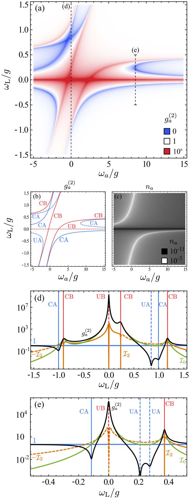
Figure 11: (Color online) Polaritonic counterpart of Fig. 7. (a) $g^{(2)}_{a}$ and (b) its structure in terms of conventional and unconventional features. CA (CB) is given by the resonant condition with the first (second) polariton manifold, cf. Eqs. (44) (for $N=1$) and (50). UA is given by the interference condition Eq. (51) and UB by $\omega_{\mathrm{L}}=0$. (c) Population $n_{a}$ and (d-e) $g^{(2)}_{a}$ (black line) for the two cuts shown in dashed lines in (a) with the cavity frequency either (d) resonant with the 2LS or (e) chosen to optimise UA ($\omega_{a}=8.63\,g$). The decomposition in $\mathcal{I}_{j}$ components is also shown, with the same conventions as in Fig. 7. Parameters: $\gamma_{a}=0.1\,g$ , $\gamma_{b}=0.01\,g$ and $U=10\gamma_{a}$.

VII.1 Conventional statistics

Like in the Jaynes-Cummings model, one can identify the conventional antibunching (CA) and bunching (CB) by mapping the observed features to an underlying blockade mechanism, namely, the positions at which $N$-photon excitation occurs, which is when the laser is resonant with one of the states in the $N$-photon rung. The first rung that provides CA is given by the same Eq. (44), with $N=1$, since this corresponds to the linear regime where both systems converge. One finds, therefore, that the two CA blue lines in Fig. 11(a), marked in solid blue in (b), are the same as in the Jaynes–Cummings model. They coincide as well with the white regions in Fig. 11(c) where the cavity emission is enhanced. This is the standard one-photon resonance, with a blockade of photons into higher rungs due to the non-linearity now introduced by the interactions (instead of the 2LS).

Higher rungs are different from the Jaynes–Cummings model, but their effects otherwise follow from the same principle and they are similarly obtained by diagonalizing the effective Hamiltonian in the corresponding $N$-excitation Hilbert subspace, that is, in the basis $\{\ket{N,0},\,\ket{N-1,1},\,\ldots\ket{0,N}\}$ (where each state is characterised by the photon and exciton number). At the two-photon level, one is interested in the second rung, which contains three eigenstates. The expressions for the general eigenenergies are rather large but we can provide here the first order in the interactions $U$ in the strong coupling limit ($g\gg\gamma_{a}$, $\gamma_{b}$):

$$E_{0}^{(2)} =\omega_{a}+\omega_{b}+\frac{g^{2}}{2R^{2}}U\,,$$ (50a)

$$E^{(2)}_{\pm} =\omega_{a}+\omega_{b}\pm 2R+\frac{2g^{2}+(\omega_{a}-\omega_{b})[(\omega_{a}-\omega_{b})\mp 2R]}{8R^{2}}U\,,$$ (50b)

with $R=\sqrt{g^{2}+(\omega_{a}-\omega_{b})^{2}/4}$ the normal mode splitting typical of strong coupling. In this limit, $E^{(1)}_{\pm}=(\omega_{a}+\omega_{b})/2\pm R$. The CB lines are positioned, therefore, according to the conditions for two-photon excitation by the laser: $\omega_{\mathrm{L}}=\Re{E_{-}^{(2)}}/2$, $\Re{E_{0}^{(2)}}/2$, $\Re{E_{+}^{(2)}}/2$, in increasing order, as they appear in Fig. 11(a), marked with solid red lines in Fig. 11(b). The upper CB line, corresponding to $E_{+}^{(2)}$, is the faintest one in the cavity emission due to the fact that it has the most excitonic component. It is monotonically blueshifted with increasing $U$ and becomes linear in the density plot as $E_{+}^{(2)}\rightarrow U$. The other two levels converge to those in the Jaynes–Cummings model in such case: $E_{-}^{(2)}\rightarrow-\sqrt{2}g$ and $E_{0}^{(2)}\rightarrow\sqrt{2}g$.

VII.2 Unconventional statistics

We now shift to the unconventional features in polariton blockade. Superbunching, or UB, is found by minimization of $\langle n_{a}\rangle$ and, therefore, also occurs for the same condition as the Jaynes–Cummings model $\Delta_{b}=\chi g\cos\phi$. The maximum superbunching is obtained at one of the crossings of UB and CB.

Now turning to the more interesting Unconventional Antibunching (UA) features, they are found, in the polariton case as well, from the minimization of $g^{(2)}_{a}$. Since the equations are quite bulky, only the case of cavity excitation ($\Omega_{b}=0$) is included here (the full expression can be consulted at App. H). The UA curve is given by the solution of

$$\Delta_{a}=-\Delta_{b}-\frac{4g^{2}\Delta_{b}}{\gamma_{b}^{2}+4\Delta_{b}^{2}}+\frac{2g^{2}(U+2\Delta_{b})}{\gamma_{b}^{2}+(U+2\Delta_{b})^{2}},$$ (51)

and the conditions for perfect antibunching come from solving the equation

$$\gamma_{b}\left[1+4g^{2}\left(-\frac{4g^{2}\Delta_{b}}{\gamma_{b}^{2}+4\Delta_{b}^{2}}+\frac{2g^{2}(U+2\Delta_{b})}{\gamma_{b}^{2}+(U+2\Delta_{b})^{2}}\right)\right]=-\gamma_{a}$$ (52)

and subsequently imposing that every parameter must be real (or the more restrictive case: real and positive) that lead to additional restrictions.

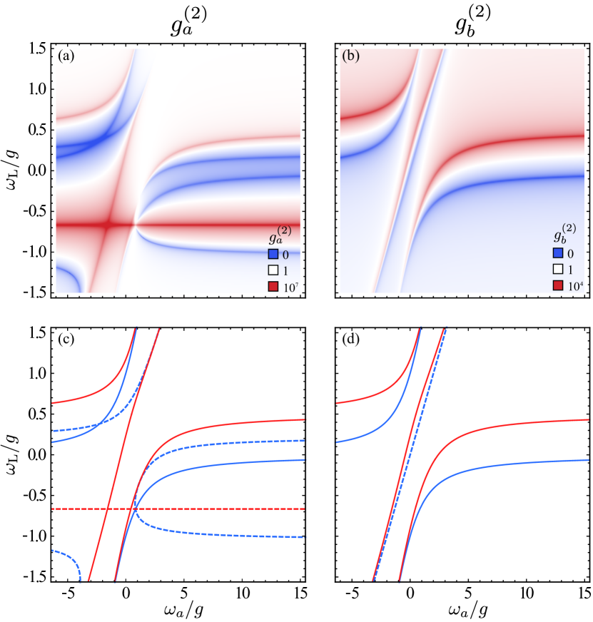
Figure 12: (Color online) Effects on the polaritonic photon statistics. Same as Fig. 11 but for (a) nonzero exciton-driving and (b) observed through the direct excitonic emission $g^{(2)}_{b}$. In the latter case, all the unconventional features have disappeared. The bottom row identifies the features through the structure of conventional and unconventional lines. Parameters: $\gamma_{a}=0.1\,g$, $\gamma_{b}=0.01\,g$, $\chi=0$ and $U=10\,\gamma_{a}$.

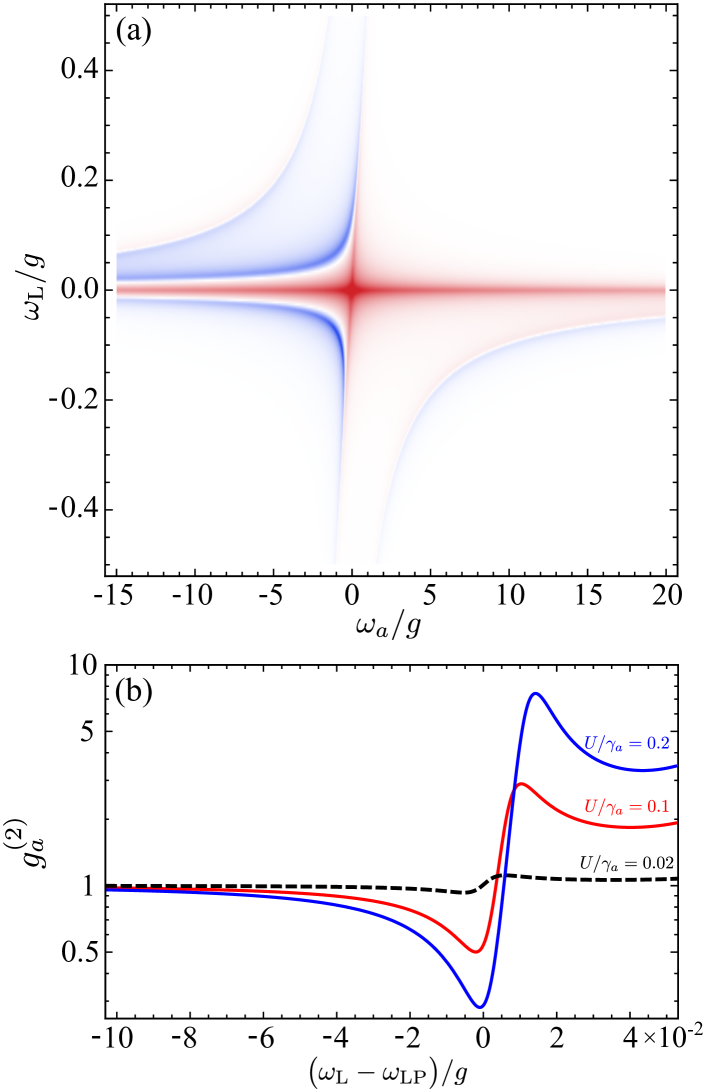
Figure 13: Polariton blockade. (a) Same as Fig. 11 but for an experimentally realistic weak value of $U/\gamma_{a}=0.1$, showing how the UB and CA lines merge into the characteristic “polariton blockade” dispersive shape shown in Panel (b) (fixed $\omega_{a}=1$, the rest of parameters have got the same value as the indicated figure).

As already noted, the polariton case adds a third CA line as compared to its Jaynes–Cummings counterpart. The correspondence between both cases is still clear, but this is largely thanks to the large interaction strength chosen in Fig. 11, namely, $U/\gamma_{a}=10$. This choice will allow us to survey quickly the polaritonic phenomenology based on the more thoroughly discussed Jaynes–Cummings one. Figure 12, for instance, shows the polaritonic counterpart of Fig. 8 on its left panel but for one case of mixed-pumping only, highlighting the considerable reshaping of the structure and the importance of controlling, or at least knowing, the ratio of exciton and photon driving. The right panel of Fig. 12 provides $g^{(2)}_{b}$, which, if compared to Fig. 11, shows that the main result is to remove all the unconventional features and retain only the conventional ones. The peaks are also less in the excitonic emission, producing a smoother background. Another dramatic feature of the excitonic correlations, which is apparent from Eq. (49), is that it is independent from the ratio $\chi$ of driving, i.e., the same result is obtained if driving the cavity alone, the exciton alone, or a mixture of both, in stark contrast of the cavity correlations (cf. Fig. 11(a) and 12(a) where the only difference is that half the excitation drives the 2LS in the second case rather than going fully to the cavity in the first case). This could be of tremendous value for spectroscopic characterization of such systems since it is typically difficult to know the exact type of pumping, while experimental evidence shows that both fields are indeed being driven under coherent excitation dominici14a . If measuring the excitonic correlations, there is no dependence from the particular type of coupling of the laser to the system. On the other hand, excitonic emission is much less straighftorward of access. Note, finally, that one could similarly consider the lower and upper polariton statistics, but they are even less featureless, with correlations of the signal that merely follow the polariton branches (their expression is given in the appendix for completeness).

Finally, in Fig. 13, we focus on the effect of the interaction strength and how to optimise the observation of antibunching. We have already emphasized that for clarity of the connection between the Jaynes–Cummings and the polariton case, we have considered a value of $U/\gamma_{a}$ substantially in excess even of the few cases themselves largely in excess of the bulk of the literature sun17b ; rosenberg18a ; togan18a . While it is not excluded that such a regime will be available in the near future, it is naturally more relevant to turn to the most common experimental configuration where $U/\gamma_{a}\ll 1$. We show such a case in Fig. 13(a), where $U/\gamma_{a}=0.1$. We see how, as a result, the CB and CA lines of the positively-detuned case collapse one onto the other. The UA line previously in between has, in the process, disappeared. The CA and CB however do not cancel each other but merge into a characteristic dispersive-like shape, shown in panel (b), the observation of which, predicted over a decade ago verger06a , has been a long-awaited result for polaritons and has indeed been just recently reported from two independent groups arXiv_delteil18a ; arXiv_munozmatutano17a . While this shape has been regarded as an intrinsic and fundamental profile of polariton blockade, our wider picture shows how it arises instead from different features brought to close proximity by the weak interactions. The difficulty in reporting polariton blockade lies in the weak value of antibunching, which is largely due to the fact that no optimisation over the full structure of photon correlations, that was unknown till this work, has been made for the driving configuration that yields the best antibunching for given system parameters.

VIII Summary, Discussion and Conclusion

We have connected an hitherto disparate and voluminous phenomenology of photon statistics in the light emitted by a variety of optical systems, into a unified picture that identifies two classes of conventional and unconventional features, covering both the cases of antibunching and bunching, which leads us to a classification of CA, UA, CB and UB. One class (conventional), linked to real states repulsion, occurs at all orders and for all photon numbers while the other (unconventional) occurs for a given photon-number with no a priori underlying level structure.

To lowest order in the driving, the dynamical response can be described by an interferences between a squeezed component and a coherent component, and thus, in this picture, one can understand the photon statistics emitted by many optical systems as simply arising from the particular way each implementation finds to produce some squeezing on the one hand and some coherent field on the other hand, and interfere them during its emission. In agreement with the previous literature, we call this phenomenon “self-homodyning”. With this understanding, one can bring considerable tailoring of photon correlations by modifying the relative importance of coherence vs squeezing, which is conveniently achieved by superimposing a fraction of the driving laser to the output of the system (“homodyning”). This Gaussian-state approximation holds to lower orders in the driving for the first correlation functions only. For instance, for the case of the laser-corrected two-level system (Table 1), the squeezed-coherent Gaussian description holds up to the second-order in the driving for the population and to the first-order in the driving for $g^{(2)}$. Deviations occur for these observables to higher-orders in the driving while higher-order correlation functions already differ to the lowest order in the driving. Such deviations seem to arise from the non-Gaussian nature of the quantum fluctuations in these highly non-linear systems. This remains to be studied in detail.

Such a general picture can explain under a unified mechanism a wealth of observations that could otherwise appear to be peculiarities that are specific to a particular configuration. To take one recent example from a group that has been leading in the development and applications of the type of homodyning and self-homodyning that we have studied above, in Ref. arXiv_trivedi19a , Trivedi et al. study the generalization of the Jaynes–Cummings system to $N$ emitters: the so-called Tavis–Cummings Hamiltonian. Here, it is found that driving resonantly the eigenstates laussy11a produces conventional antibunching, flanked by unconventional antibunching for laser frequencies detuned from the one- and two-photon resonances. This is the counterpart of the situation of Fig. 7(d) (resonance) and (e) (detuning), both also shown in Panel (a), where increasing $N$ has the effect of bosonizing the interacting (matter-like) part of the system or decreasing the effective nonlinearity, similarly to decreasing $g$ for $N=1$. Interestingly, it is reported that while for the case of resonance, antibunching is spoiled with an increasing number of emitters $N$, in presence of a detuning, one of the antibunching peaks is, on the opposite, enhanced with increasing $N$. This apparently puzzling behaviour is easily understood once the conventional and unconventional nature of the respective antibunching lines are recognized. In the resonant case, antibunching is always conventional, and as such it is spoiled by the bosonization of the system due to it increasing number of emitters dicke54a , or by reducing the coupling. Since both weaken the nonlinearity in the level structure, this destroys the conventional blockade that is based on it. With detuning, on the other hand, one finds not only conventional but also unconventional antibunching, cf. Fig. 7(b). Their CA is also spoiled with increasing $N$, as reported, but their UA, however, increases, which can be expected since it is due to an self-homodyning interference between the coherent and incoherent parts of the emission at the two-photon level, as explained above, and this does not suffer from a reduced nonlinearity (or increasing $N$). It can in fact be also optimized (i.e., reduced) like all types of UA and as a result, should even reach $g^{(2)}=0$ to lowest order for a proper choice of the detuning, that will depend on $N$ in a way that remains to be computed. Since we have shown, however, that the interference nature of UA makes it sensitive to dephasing, and that detuning lopezcarreno19a results in fast oscillations in autocorrelation times, with a narrowing plateau of antibunching, one can also expect this antibunching to be particularly fragile and difficult to resolve when including a realistic model for its detection. This is consistent with the finding of the Authors that inhomogeneous broadening quickly spoils UA. Finally, they also find in both detuned and resonant cases the unconventional bunching, as the large bunching central peak that is a typical feature of the general mechanism (cf. Fig. 7). This is therefore the super-chaotic noise due to self-homodyning stripping down the emission to its mere fluctuations. As such, the interpretation in terms of two-photon bound states that is offered in Ref. arXiv_trivedi19a and in other works faraon08a ; dory17a should be further analyzed and quantified. We suspect the emission in UB to be less efficient for multiphoton Physics as compared to leapfrog emission sanchezmunoz14a , due to the lack of a suppression mechanism for higher photon-number processes, and despite the large values of the correlation functions that they produce.

As a conclusion, our picture brings considerable simplification in the interpretation and identification of the various phenomena observed in a plethora of systems, in particular with respect to connecting them between each other throughout platforms. It clarifies the value but also the limitation of a description in terms of Gaussian-states. It also opens a new route to control and fine-tune such photon correlations and make a more informed and better use of them for quantum applications.

Appendices

Appendix A Interference between a coherent and squeezed state.

In a beam splitter (with a certain transmittance $\mathrm{T}^{2}$ and reflectance $\mathrm{R}^{2}$), the relation between the input light fields ($a$, $d$) and the output fields ($o$, $s$) is a simple unitary transformation:

$$o=\mathrm{T}d+i\mathrm{R}a\,,\quad s=i\mathrm{R}d+\mathrm{T}a\,,\quad\text{and}\quad d=\mathrm{T}o-i\,\mathrm{R}s\,,\quad a=-i\,\mathrm{R}o+\mathrm{T}s\,,$$ (1)

where the real coefficients $\mathrm{T}$ and $\mathrm{R}$ must fulfil $1\geq\mathrm{T},\mathrm{R}\geq 0$ and $\mathrm{T}^{2}+\mathrm{R}^{2}=1$. In our case of interest, the input 0 is a squeezed state $\ket{\xi}=\mathcal{S}_{d}\left(\xi\right)\ket{0}$ and input 1, a coherent state $\ket{\alpha}=\mathcal{D}_{a}\left(\alpha\right)\ket{0}$. The squeezing operator is $\mathcal{S}_{d}\left(\xi\right)=\exp\left[\frac{1}{2}\left(\xi^{*}d^{2}-\xi{d^{\dagger}}^{2}\right)\right]$ with squeezing parameter $\xi=re^{i\theta}$ and the displacement operator is $\mathcal{D}_{a}\left(\alpha\right)=\exp\left(\alpha{a^{\dagger}}-\alpha^{*}a\right)$ with coherent parameter $\alpha=|\alpha|e^{i\phi}$. The total input state can be written as:

$$\ket{\psi_{\mathrm{in}}}=\mathcal{D}_{a}\left(\alpha\right)\mathcal{S}_{d}\left(\xi\right)\ket{0}_{da},$$ (2)

where the state subscript indicates the input/output subspaces where operators are acting upon. These operators are written in the input basis. Now, applying transformations of Eq. (1) and rearranging terms, we obtain, in first place, for the displacement operator: $\mathcal{D}_{a}\left(\alpha\right)=\exp\left(\alpha{o^{\dagger}}-\alpha^{*}o+\alpha{s^{\dagger}}-\alpha^{*}s\right)$, where $\alpha_{o}=i\mathrm{R}\alpha$ and $\alpha_{s}=\mathrm{T}\alpha$. Exponentials of operators can be factorized since both output are independent from each other and commute. This leads to the simple expression: $\mathcal{D}_{a}\left(\alpha\right)=\mathcal{D}_{o}\left(\alpha_{o}\right)\mathcal{D}_{s}\left(\alpha_{s}\right)=\mathcal{D}_{s}\left(\alpha_{s}\right)\mathcal{D}_{o}\left(\alpha_{o}\right)$, where each displacement operator $\mathcal{D}_{j}\left(\alpha_{j}\right)$ ($j=o,s$) only acts over the assigned output. Then, the squeezing operator in the output basis reads:

$$\mathcal{S}_{d}\left(\xi\right)=\exp\left[\frac{1}{2}\left(\xi_{o}^{*}o^{2}-\xi_{o}{o^{\dagger}}\right)+\frac{1}{2}\left(\xi_{s}^{*}s^{2}-\xi_{s}{s^{\dagger}}\right)+\right.\left.\left(\xi_{os}^{*}os-\xi_{os}{o^{\dagger}}{s^{\dagger}}\right)\right]=\exp(S_{o}+S_{s}+S_{os})\,,$$ (3)

where $\xi_{o}=\mathrm{T}^{2}\xi$, $\xi_{s}=-\mathrm{R}^{2}\xi$ and $\xi_{os}=i\mathrm{R}\mathrm{T}\,\xi$. This exponential can be simply split into two different contributions only if $[S_{o}+S_{s},S_{os}]=0$, which is fulfilled only in the particular case $\mathrm{T}=\mathrm{R}$ (symmetrical BS). Although this constriction could suppose a huge difficulty to overcome, first correction term grows proportional to $r^{2}\mathrm{T}\mathrm{R}\left(\mathrm{T}^{2}-\mathrm{R}^{2}\right)$. Thus, for either low squeezing signal ($r\ll 1$) or almost symmetrical BS ($\mathrm{T}-\mathrm{R}\approx 0$), the output signal could be described as follows. The commutator $[S_{o},S_{s}]$ vanishes for any possible values, so the exponential simplifies into $\mathcal{S}_{d}\left(\xi\right)=\mathcal{S}_{o}\left(\xi_{o}\right)\mathcal{S}_{s}\left(\xi_{s}\right)\mathcal{S}_{os}\left(\xi_{os}\right)$. With the previous results, the output state can be written as:

$$\ket{\psi_{\mathrm{out}}}=\mathcal{D}_{o}\left(\alpha_{o}\right)\mathcal{S}_{o}\left(\xi_{o}\right)\mathcal{D}_{s}\left(\alpha_{s}\right)\mathcal{S}_{s}\left(\xi_{s}\right)\mathcal{S}_{os}\left(\xi_{os}\right)\ket{0}_{os}\\ =\mathcal{D}_{o}\left(\alpha_{o}\right)\mathcal{S}_{o}\left(\xi_{o}\right)\mathcal{D}_{s}\left(\alpha_{s}\right)\mathcal{S}_{s}\left(\xi_{s}\right)\ket{\xi_{os}}_{os},$$ (4)

where $\ket{\xi_{os}}$ represents a two-mode squeezed state. In the Fock basis, this state can be written as (from Ref. guerry_book05a , Chapter 7):

$$\ket{\xi_{os}}=\frac{1}{\cosh r_{os}}\sum_{n=0}^{\infty}\left(\tanh r_{os}\right)^{n}\ket{n,n}_{os},$$ (5)

where $r_{os}=|\xi_{os}|=\mathrm{R}\mathrm{T}\,r$. The corresponding density matrix for this pure state reads $\rho_{\mathrm{out}}=\ket{\psi_{\mathrm{out}}}\bra{\psi_{\mathrm{out}}}$. Tracing out output $o$, we obtain the density matrix for output $s$ only (our signal of interest): $\rho_{s}=\Tr_{o}\{\rho_{\mathrm{out}}\}$. For the next step, we will use the properties of the trace to move clockwise the operators acting over the output $o$ subspace and the identities ${\mathcal{D}_{o}^{\dagger}}\left(\alpha_{o}\right)\mathcal{D}_{o}\left(\alpha_{o}\right)={\mathcal{S}_{o}^{\dagger}}\left(\xi_{o}\right)\mathcal{S}_{o}\left(\xi_{o}\right)=\hat{\mathds{1}}_{o}$, where $\hat{\mathds{1}}_{o}$ is the identity operator. Furthermore, any operator that only acts on the $s$-subspace can be taken out of the trace. With this,

$$\rho_{s}=\mathcal{D}_{s}\left(\alpha_{s}\right)\mathcal{S}_{s}\left(\xi_{s}\right)\big{(}\Tr_{o}\{\ket{\xi_{os}}\bra{\xi_{os}}\}\big{)}{\mathcal{S}_{s}^{\dagger}}\left(\xi_{s}\right){\mathcal{D}_{s}^{\dagger}}\left(\alpha_{s}\right)\,.$$ (6)

Computing the partial trace:

$$\begin{split}\Tr_{o}\{\ket{\xi_{os}}\bra{\xi_{os}}\}=&\sum_{p=0}^{\infty}\bra{p}_{o}\left(\frac{1}{\cosh^{2}r_{os}}\sum_{n,m=0}^{\infty}\left(\tanh r_{os}\right)^{n+m}\ket{n}_{o}\ket{n}_{s}\bra{m}_{s}\bra{m}_{o}\right)\ket{p}_{o}\\ =&\,\frac{1}{\cosh^{2}r_{os}}\sum_{n}^{\infty}\left(\tanh r_{os}\right)^{2n}\ket{n}_{s}\bra{n}_{s},\end{split}$$ (7)

from the second to the third equality we have used $\innerproduct{m}{p}_{o}=\delta_{m,p}$ and $\innerproduct{p}{n}_{o}=\delta_{p,n}$. The resulting density matrix has the form of a thermal state $\rho_{\mathrm{th}}$ with mean population $\mathrm{p_{th}}\equiv\langle{s^{\dagger}}s\rangle_{\mathrm{th}}=\sinh^{2}r_{os}$. To sum up, the output field detected at a single arm of the system corresponds to a displaced squeezed thermal state. So, to sum up,

$$\rho_{s}=\mathcal{D}_{s}\left(\alpha_{s}\right)\mathcal{S}_{s}\left(\xi_{s}\right)\rho_{\mathrm{th}}{\mathcal{S}_{s}^{\dagger}}\left(\xi_{s}\right){\mathcal{D}_{s}^{\dagger}}\left(\alpha_{s}\right),$$ (8)

with parameters $\alpha_{s}=\mathrm{T}|\alpha|e^{i\phi}$, $\xi_{s}=r_{s}e^{i\theta_{s}}=\mathrm{R}^{2}e^{i\left(\theta+\pi\right)}$ and $\mathrm{p_{th}}=\sinh[2](\mathrm{R}\mathrm{T}\,r)$. Even though $\mathrm{T}$ and $\mathrm{R}$ appear as parameters, last equation only works for $\mathrm{R}\approx\mathrm{T}$. We restrict ourselves to the case of 50:50 beam splitter ($\mathrm{T}^{2}=\mathrm{R}^{2}=1/2$). Thermal population can be expressed in terms of squeezed population of the input signal $\langle n_{d}\rangle=\sinh^{2}r$:

$$\mathrm{p_{\mathrm{th}}}+\frac{1}{2}=\frac{1}{2}\sqrt{1+\langle n_{d}\rangle}.$$ (9)

From $\rho_{s}$ we can compute the observables for the mixed signal:

$$\langle n_{s}\rangle=\frac{|\alpha|^{2}}{2}+\frac{\langle n_{d}\rangle}{2}\,,\quad|\langle s^{2}\rangle|=\left(\mathrm{p_{th}}+\frac{1}{2}\right)\sinh(r)\,,$$ (10a)

$$g^{(2)}_{s}=1+\langle n_{s}\rangle^{-2}\sinh^{2}r\left[\cosh 2r+2|\alpha|^{2}\left(1-\cos(\theta-2\phi)\coth r\right)\right]\,,$$ (10b)

$$g^{(3)}_{s}=1+\langle n_{s}\rangle^{-3}\sinh^{2}r\,\Big{\{}\sinh^{2}2r+5\sinh^{2}r\cosh 2r+6|\alpha|^{4}\left(1-\cos(\theta-2\phi)\coth r\right)+\\ \>3|\alpha|^{2}\left[3\coth^{2}r-1+6\left(1-\cos(\theta-2\phi)\coth r\right)\right]\Big{\}}\,,$$ (10c)

Appendix B Decomposition of $g_{s}^{(3)}$ in powers $\alpha$

We provide the third-order coherence function of signal $s$, in terms of two interfering fields, $s=\alpha+d$. As in the case for $g^{(2)}_{s}$, the highest order contributions in powers of $\alpha$ can be gathered into the coherent term (given by 1), yielding:

$$g^{(3)}_{s}=1+\sum_{m=0}^{4}\mathcal{J}_{m}\,,$$ (11)

with

$$\mathcal{J}_{0} =\frac{\langle d^{\dagger 3}d^{3}\rangle-\langle{d^{\dagger}}d\rangle^{3}}{\langle n_{s}\rangle^{3}}\,,$$ (12)

$$\mathcal{J}_{1} =6\frac{\real[\alpha^{*}\left(\langle d^{\dagger 2}d^{3}\rangle-\langle d\rangle\langle{d^{\dagger}}d\rangle\right)]}{\langle n_{s}\rangle^{3}}\,,$$ (13)

$$\mathcal{J}_{2} =3\Big{[}2\real[{\alpha^{*}}^{2}\langle{d^{\dagger}}d^{3}\rangle]+|\alpha|^{2}\left(3\langle d^{\dagger 2}d^{2}\rangle+\langle{d^{\dagger}}d\rangle^{2}\right)-4\real[\alpha^{*}\langle d\rangle]^{2}\Big{]}/\langle n_{s}\rangle^{3}\,,$$ (14)

$$\mathcal{J}_{3} =2\Big{[}\real[{\alpha^{*}}^{3}\langle d^{3}\rangle]+|\alpha|^{2}\real[\alpha^{*}\left(9\langle{d^{\dagger}}d^{2}\rangle-\langle d\rangle\langle{d^{\dagger}}d\rangle\right)]-4\real[\alpha^{*}\langle d\rangle]^{3}\Big{]}/\langle n_{s}\rangle^{3}\,,$$ (15)

$$\mathcal{J}_{4} =6|\alpha|^{2}\frac{\real[{\alpha^{*}}^{2}\langle d^{2}\rangle]+|\alpha|^{2}\langle{d^{\dagger}}d\rangle-2\real[\alpha^{*}\langle d\rangle]^{2}}{\langle n_{s}\rangle^{3}}\,.$$ (16)

Appendix C Coherent and squeezed steady states

The coherent and the squeezed state described in Sec. (III) can be obtained as the steady-state solutions of a driven cavity, described through the master equation (hereafter $\hbar=1$ is assumed)

$$\partial_{t}\rho=i[\rho,H_{c}]+\frac{\gamma_{c}}{2}\mathcal{L}_{c}\rho\,.$$ (17)

Here $\mathcal{L}_{c}=(2c\rho{c^{\dagger}}-{c^{\dagger}}c\rho-\rho{c^{\dagger}}c)$ and $c=a,d$ are the annihilation operator of the field generating the coherent and squeezed state. The Hamiltonians are set as $H_{a}=\Delta_{a}{a^{\dagger}}a+\Omega_{a}({a^{\dagger}}+a)$ for the coherent state and $H_{d}=\Delta_{d}{d^{\dagger}}d+\lambda_{d}(d^{\dagger 2}+d^{2})$ for the squeezed state. In the former case, $\Delta_{a}$ is the detuning between the cavity and the laser that excites the cavity with intensity $\Omega_{a}$ and in the latter case, it is the detuning between the cavity and the driving mode that squeezes the cavity with intensity $\lambda_{d}$. The relation between the dynamical quantities and the displacement and the squeezing parameters is the following: $\alpha=\langle a\rangle$, $\sinh^{2}(r)=\langle{d^{\dagger}}d\rangle$ and $\tan\theta=i(\langle d^{\dagger 2}\rangle-\langle d^{2}\rangle)/(\langle d^{\dagger 2}\rangle+\langle d^{2}\rangle)$. These two systems can be solved exactly, so the steady-state solutions for the parameters defined above are:

$$|\alpha|=\frac{2\Omega_{a}}{\sqrt{\gamma_{a}+4\Delta_{a}^{2}}}\quad\text{and}\quad\tan\phi=-\frac{\gamma_{a}}{2\Delta_{a}}\,,$$ (18)

for the coherent state and

$$\tanh(2r)=\frac{4\lambda_{d}}{\sqrt{\gamma_{d}^{2}+4\Delta_{d}^{2}}}\quad\text{and}\quad\tan\theta=\frac{\gamma_{d}}{2\Delta_{d}}\,,$$ (19)

for the squeezed state. For the latter case, there is also a thermal contribution given by $\mathrm{p_{th}}=\sinh[2](r)$, so the resulting state is actually a thermal squeezed state.

Appendix D Steady states of light matter coupling at vanishing laser driving

In this work we need to solve the steady state dynamics of light-matter interaction in the low coherent driving regime. The light field is a cavity mode $a$ and the matter field can be either a 2LS $\sigma$ or another bosonic mode $b$. We solve the dynamics in terms of a general mean value, a product of any system operator, which in its most general normally ordered form reads $C_{\{m,n,\mu,\nu\}}=\langle\sigma^{\dagger m}\sigma^{n}a^{\dagger\mu}a^{\nu}\rangle$ (with $m$, $n\in\{0,1\}$ and $\mu$, $\nu\in\mathbb{N}$) if the matter field is a 2LS or  $C_{\{m,n,\mu,\nu\}}=\langle b^{\dagger m}b^{n}a^{\dagger\mu}a^{\nu}\rangle$ (with $m$, $n$, $\mu$, $\nu\in\mathbb{N}$) if the matter field is bosonic. This general element follows the master equation described in the main text, which can be expressed in a matricial form:

$$\partial_{t}C_{\{m,n,\mu,\nu\}}=\sum_{{m^{\prime},n^{\prime},\mu^{\prime},\nu^{\prime}}}\mathcal{M}_{\begin{subarray}{c}m,n,\mu,\nu\\ m^{\prime},n^{\prime},\mu^{\prime},\nu^{\prime}\end{subarray}}C_{\{m^{\prime},n^{\prime},\mu^{\prime},\nu^{\prime}\}}\,.$$ (20)

The regression matrix elements $\mathcal{M}_{\begin{subarray}{c}m,n,\mu,\nu\\ m^{\prime},n^{\prime},\mu^{\prime},\nu^{\prime}\end{subarray}}$, in the case of a coupled 2LS, are given by:

$$\mathcal{M}_{\begin{subarray}{c}m,n,\mu,\nu\\ m,n,\mu,\nu\end{subarray}}=-\frac{\gamma_{a}}{2}(\mu+\nu)-\frac{\gamma_{\sigma}}{2}(m+n)+i(\mu-\nu)\delta_{a}+i(m-n)\Delta_{\sigma}$$ (21a)

$$\mathcal{M}_{\begin{subarray}{c}m,n,\mu,\nu\\ 1-m,n,\mu,\nu\end{subarray}}=i\Omega_{\sigma}[m+2n(1-m)]\,,\quad \mathcal{M}_{\begin{subarray}{c}m,n,\mu,\nu\\ m,1-n,\mu,\nu\end{subarray}}=-i\Omega_{\sigma}[n+2m(1-n)]\,$$ (21b)

$$\mathcal{M}_{\begin{subarray}{c}m,n,\mu,\nu\\ m,n,\mu-1,\nu\end{subarray}}=i\Omega_{a}\mu\,,\quad \mathcal{M}_{\begin{subarray}{c}m,n,\mu,\nu\\ m,n,\mu,\nu-1\end{subarray}}=-i\Omega_{a}\nu\,,$$ (21c)

$$\mathcal{M}_{\begin{subarray}{c}m,n,\mu,\nu\\ m,1-n,\mu,\nu-1\end{subarray}}=-ig(1-n)\nu\,,\quad \mathcal{M}_{\begin{subarray}{c}m,n,\mu,\nu\\ 1-m,n,\mu-1,\nu\end{subarray}}=ig(1-m)\mu\,,$$ (21d)

$$\mathcal{M}_{\begin{subarray}{c}m,n,\mu,\nu\\ m,1-n,\mu,\nu+1\end{subarray}}=-ign\,,\quad \mathcal{M}_{\begin{subarray}{c}m,n,\mu,\nu\\ 1-m,n,\mu+1,\nu\end{subarray}}=igm\,,$$ (21e)

$$\mathcal{M}_{\begin{subarray}{c}m,n,\mu,\nu\\ 1-m,n,\mu,\nu+1\end{subarray}}=2ing(1-m)\,,\quad \mathcal{M}_{\begin{subarray}{c}m,n,\mu,\nu\\ m,1-n,\mu+1,\nu\end{subarray}}=-2ing(1-m)\,,$$ (21f)

and zero everywhere else. In the main text, we discuss first the case of resonance fluorescence, which corresponds to having only the 2LS operator $\sigma$ and no cavity mode $a$ (taking $g$, $\Omega_{a}=0$ here). Second, we solve the Jaynes–Cummings model with both cavity and dot driving with a phase difference between the sources, which corresponds to setting $\Omega_{\sigma}/\Omega_{a}=\chi e^{-i\phi}$ here.

Similarly, for the polariton model where the matter field is an exciton (boson), we have:

$$\mathcal{M}_{\begin{subarray}{c}m,n,\mu,\nu\\ m,n,\mu,\nu\end{subarray}}=-\frac{\gamma_{a}}{2}(\mu+\nu)-\frac{\gamma_{b}}{2}(m+n)+i(\mu-\nu)\Delta_{a}+i(m-n)\Delta_{b}+i\frac{U}{2}\left[m(m-1)-n(n-1)\right],$$ (22a)

$$\mathcal{M}_{\begin{subarray}{c}m,n,\mu,\nu\\ m,n,\mu-1,\nu\end{subarray}}=i\Omega_{a}\mu, \mathcal{M}_{\begin{subarray}{c}m,n,\mu,\nu\\ m,n,\mu,\nu-1\end{subarray}}=-i\Omega_{a}\nu\,$$ (22b)

$$\mathcal{M}_{\begin{subarray}{c}m,n,\mu,\nu\\ m+1,n,\mu-1,\nu\end{subarray}}=ig\mu\,,\quad \mathcal{M}_{\begin{subarray}{c}m,n,\mu,\nu\\ m,n+1,\mu,\nu-1\end{subarray}}=-ig\nu\,,$$ (22c)

$$\mathcal{M}_{\begin{subarray}{c}m,n,\mu,\nu\\ m-1,n,\mu+1,\nu\end{subarray}}=igm\,,\quad \mathcal{M}_{\begin{subarray}{c}m,n,\mu,\nu\\ m,n-1,\mu,\nu+1\end{subarray}}=-ign\,,$$ (22d)

$$\mathcal{M}_{\begin{subarray}{c}m,n,\mu,\nu\\ m+1,n+1,\mu,\nu\end{subarray}}=iU(m-n),\quad$$ (22e)

and, again, the remaining matrix elements are zero.

These equations can be solved numerically, by choosing a high enough truncation in the number of excitations, in order to obtain the steady state ($\partial_{t}C_{\{m,n,\mu,\nu\}}=0$) for any given pump. However, we are interested in an analytical solution when applying vanishing driving limit ($\Omega_{\sigma}\rightarrow 0$ or $\Omega_{a}\rightarrow 0$). In this case, it is enough to solve recursively sets of truncated equations. That is, we start with the lowest order correlators, with only one operator, that we write in a vectorial form for convenience (using the JC model as an example): $\mathbf{v}_{1}=(\langle a\rangle~{}\langle a^{\dagger}\rangle~{}\langle\sigma\rangle~{}\langle\sigma^{\dagger}\rangle)^{\mathrm{T}}$. Its equation, $\partial_{t}\mathbf{v}_{1}=M_{1}\mathbf{v}_{1}+A_{1}+~{}\mathrm{h.~{}o.~{}t.}$, provides the steady state value $\mathbf{v}_{1}=-M_{1}^{-1}A_{1}+~{}\mathrm{h.~{}o.~{}t.}$, to lowest order in $\Omega_{a}$ (with h. o. t. meaning higher order terms). We proceed in the same way with the two-operator correlators $\mathbf{v}_{2}=(\langle a^{2}\rangle~{}\langle a^{\dagger 2}\rangle~{}\langle a^{\dagger}a\rangle~{}\langle\sigma^{\dagger}\sigma\rangle~{}\langle\sigma^{\dagger}a\rangle\,\ldots)^{\mathrm{T}}$, only, in this case, we also need to include the steady state value for the one-operator correlators as part of the independent term in the equation: $\partial_{t}\mathbf{v}_{2}=M_{2}\mathbf{v}_{2}+A_{2}+X_{21}\mathbf{v}_{1}+~{}\mathrm{h.~{}o.~{}t.}$. The steady state reads $\mathbf{v}_{2}=-M_{2}^{-1}(A_{2}+X_{21}\mathbf{v}_{1})+~{}\mathrm{h.~{}o.~{}t.}$ with an straightforward generalization $\mathbf{v}_{N}=-M_{N}^{-1}(A_{N}+\sum_{j=1}^{N-1}X_{Nj}\mathbf{v}_{j})+~{}\mathrm{h.~{}o.~{}t.}$.

We, in particular, aim at obtaining photon correlators of the type $\langle a^{\dagger N}a^{N}\rangle$ that follow $\langle a^{\dagger N}a^{N}\rangle\sim(\Omega_{a})^{2N}$, to lowest order in the driving $\Omega_{a}$. The normalized correlation functions $g_{a}^{(N)}=\langle a^{\dagger N}a^{N}\rangle/\langle a^{\dagger}a\rangle^{N}$ are independent of $\Omega_{a}$ to lowest order, their computation requiring to solve the $2N$ sets of recurrent equations and taking the limit $\lim_{\Omega_{a}\rightarrow 0}g_{a}^{(N)}$.

Appendix E Homodyne interference with resonance fluorescence: correlations and squeezing from the fluctuations and the total signal

The correlations from the fluctuations of resonance fluorescence, with operator $\epsilon=\sigma-\alpha$, can be accessed using the technique of homodyne detection explained in Sec. (III). In this case, we feed one of the beam splitter arms with resonance fluorescence ($d\rightarrow\sigma$) and the other with a coherent field ($a\rightarrow\beta$). The correlators of the output of the arms as defined in Appendix A, $s=i\mathrm{R}\beta+\mathrm{T}\sigma$, are given by:

$$\langle s^{\dagger n}s^{m}\rangle=\sum_{p=0}^{n}\sum_{q=0}^{m}\binom{n}{p}\binom{m}{q}(-i\mathrm{R}\beta^{*})^{n-p}(i\mathrm{R}\beta)^{m-q}\langle\sigma^{\dagger p}\sigma^{q}\rangle\,.$$ (23)

Since $\langle\sigma^{\dagger p}\sigma^{q}\rangle=0$ for $p,q>1$, this simplifies to

$$\langle s^{\dagger n}s^{m}\rangle=(-i\mathrm{R}\beta^{*})^{n}(i\mathrm{R}\beta)^{m}-i\mathrm{R}\mathrm{T}\ (-i\mathrm{R}\beta^{*})^{n-1}(i\mathrm{R}\beta)^{m-1}\left(m\beta\langle\sigma\rangle-n\beta^{*}\langle\sigma\rangle^{*}\right)+nm\ (-i\mathrm{R}\beta^{*})^{n-1}(i\mathrm{R}\beta)^{m-1}\mathrm{T}^{2}\langle n_{\sigma}\rangle\,.$$ (24)

For instance, the coherent fraction and total population of the output field are:

$$\langle s\rangle =i\mathrm{R}\beta+\mathrm{T}\langle\sigma\rangle\,,$$ (25a)

$$\langle{s^{\dagger}}s\rangle =\mathrm{R}|\beta|^{2}+\mathrm{T}^{2}\langle n_{\sigma}\rangle+2\mathrm{R}\mathrm{T}\real[i\beta^{*}\langle\sigma\rangle]\,.$$ (25b)

Therefore, we can chose the coherent field to compensate exactly the coherent component of the 2LS $\alpha=\langle\sigma\rangle$, i.e., setting $\beta=i\frac{\mathrm{T}}{\mathrm{R}}\langle\sigma\rangle$ so that we hace only the transmitted fluctuations $s=T\epsilon$. In such a case the correlators simplify even further,

$$\langle\epsilon^{\dagger n}\epsilon^{m}\rangle=\langle s^{\dagger n}s^{m}\rangle/\mathrm{T}^{n+m}=(-1)^{m+n}\alpha^{m-1}\alpha^{*(n-1)}\left[nm\ \langle n_{\sigma}\rangle-\left(n+m-1\right)\big{|}\alpha\big{|}^{2}\right]\,.$$ (26)

With this general expression, we obtain the population and coherence functions, Eq. (22) of the main text.

We want to recover and analyse light properties from the original 2LS (before the beam splitter). In order to do this, the factor $\mathrm{T}^{2}$ on the population should be eliminated (making $\mathrm{T}^{2}\langle n_{\sigma}\rangle\rightarrow\langle n_{\sigma}\rangle$, $\mathrm{T}\langle\sigma\rangle\rightarrow\langle\sigma\rangle$). Note that this change is not inconsistent, given that the beam splitter divides by two the incoming signal and thus merely attenuating it by a factor $\mathrm{T}^{2}$. Moreover, since the photon correlations are normalized objects, a global attenuation in the unnormalized correlators do not change them. However, suppressing the coherent contribution of the emission is not the only possibility. We can also tune the coherent contribution by choosing $\beta^{\prime}=e^{i\phi}|\beta^{\prime}|$, where the amplitude is parametrize as $|\beta^{\prime}|=\frac{\mathrm{R}}{\mathrm{T}}|\beta|$. Thus, we are broadening the range of possible output configurations lopezcarreno18b . So, for the most general case, the $N$-particle correlators have the following form:

$$g^{(N)}_{s}=\frac{|\beta^{\prime}|^{2(n-1)}\left(|\beta^{\prime}|^{2}+n^{2}\langle n_{\sigma}\rangle+2n\imaginary\{\langle\sigma\rangle|\beta^{\prime}|e^{-i\phi}\}\right)}{\left(|\beta^{\prime}|^{2}+\langle n_{\sigma}\rangle+2\imaginary\{\langle\sigma\rangle|\beta^{\prime}|e^{-i\phi}\}\right)^{n}},$$ (27)

After this general expression, the amplitude $|\beta^{\prime}|$ is usually expressed in a more suitable way, referencing it to the driving intensity of the laser: $|\beta^{\prime}|=\frac{\Omega_{\sigma}}{\gamma_{\sigma}}\mathcal{F}$.

Other two important quantities are the mean and variance of the quadratures, $\langle X_{s,\chi}\rangle=\frac{1}{2}(e^{i\chi}\langle{s^{\dagger}}\rangle+\mathrm{c.c.})$ and their dispersion $\langle\Delta X_{s,\chi}^{2}\rangle=\langle X_{s,\chi}^{2}-\langle X_{s,\chi}\rangle^{2}\rangle$, respectively:

$$\langle X_{s,\chi}\rangle=\frac{1}{2}\left(e^{i\phi}\langle s\rangle^{*}+\mathrm{c.c}\,\right),$$ (28)

The mean value only depends on the total coherent contribution $\langle s\rangle=\mathrm{T}(i\beta^{\prime}+\alpha)$.

The maximum and minimum of the (normal-ordered) quadrature variance for a single-mode can be inferred independently of specific nature of the field:

$$\langle:\Delta X_{s}^{2}:\rangle_{\mathrm{max}/\mathrm{min}}=\langle\Delta X_{s}^{2}\rangle_{\mathrm{max}/\mathrm{min}}-\frac{1}{4}=\frac{1}{2}\left[\pm|\langle s^{2}\rangle-\langle s\rangle^{2}|+\langle{s^{\dagger}}s\rangle-|\langle s\rangle|^{2}\right],$$ (29)

where the sign correspond to maximum and minimum, respectively. While the variance is strictly a positive-valued quantity, its normal-ordered counterpart is not. This latter indicates the deviation of the variance from the vacuum value (which is $\frac{1}{4}$) so values below 0 will reveal some degree of quadrature squeezing. Likewise the angle of squeezing is generically given by:

$$\theta=\mathrm{arg}\left[\langle s^{2}\rangle-\langle s\rangle^{2}\right].$$ (30)

After substituting the correlators (26) on (29) and, then, using the steady-state solution given in Eq. (18):

$$\langle:\Delta X_{s}^{2}:\rangle_{\mathrm{min}}=-\frac{2\mathrm{T}^{2}\Omega_{\sigma}^{2}\left(\gamma_{\sigma}^{2}+4\Delta_{\sigma}^{2}-8\Omega_{\sigma}^{2}\right)}{\left(\gamma_{\sigma}^{2}+4\Delta_{\sigma}^{2}+8\Omega_{\sigma}^{2}\right)^{2}}, \ \ \langle:\Delta X_{s}^{2}:\rangle_{\mathrm{max}}=\frac{2\mathrm{T}^{2}\Omega_{\sigma}^{2}}{\gamma_{\sigma}^{2}+4\Delta_{\sigma}^{2}+8\Omega_{\sigma}^{2}},$$ (31)

and the angle of squeezing will be:

$$\theta=\mathrm{arg}\left[\left(\gamma_{\sigma}-2i\Delta_{\sigma}\right)^{2}\right]$$ (32)

It is not surprising that factor $\mathcal{F}$ does not appear since all the squeezing properties exclusively come from the fluctuations. The strength of this effect is reduced by the factor $\mathrm{T}^{2}$ as the input signal $\sigma$ ($\alpha+\epsilon$) is divided by the beam splitter, which can naturally absorbed into $\Omega_{\sigma}^{2}$. Now we are interested in the low driving regime ($\Omega_{\sigma}\rightarrow 0$), so the previous expressions at the lowest order in $\Omega_{\sigma}$ simplify

$$\langle:\Delta X^{2}_{s}:\rangle_{\mathrm{max}/\mathrm{min}}\approx\pm\frac{2\Omega_{\sigma}^{2}}{\gamma_{\sigma}^{2}+4\Delta^{2}_{\sigma}},$$ (33)

In this limit, both dispersion are symmetrical (but with opposite signs). We can regard these expression as a limit of low squeezing (and coherent intensity $|\alpha|^{2}$) from a displaced squeezed thermal state (although the coherent part does not contribute to the variance). Such states has got the following dispersion when $r\rightarrow 0$:

$$\langle:\Delta X^{2}:\rangle_{\mathrm{max}/\mathrm{min}}^{\mathrm{DST}}\approx\frac{1}{4}\left[\left(1\pm 2r\right)\left(1+2\langle n_{\mathrm{th}}\rangle\right)-1\right]\approx\pm\,\frac{r}{2},$$ (34)

where the superscript on the average reminds that the observable corresponds to an displaced squeezed thermal state. We have approximated $1+2\langle n_{\mathrm{th}}\rangle$ as $1$ since the thermal population grows like $\Omega_{\sigma}^{4}$ (which comes from the first order of the incoherent population). Comparing (33) with (34), we found that the incoherent population in the Heitler regime behaves like a squeezed thermal state with squeezing parameter

$$r_{\mathrm{eff}}=\frac{4\Omega_{\sigma}^{2}}{\gamma_{\sigma}^{2}+4\Delta_{\sigma}^{2}},$$ (35)

and the effective thermal population $\mathrm{p}_{\mathrm{th}}$:

$$\mathrm{p}_{\mathrm{th}}\approx\frac{16\Omega_{\sigma}^{4}}{\left(\gamma_{\sigma}^{2}+4\Delta_{\sigma}^{2}\right)^{2}},$$ (36)

From these two parameters an effective $g^{(2)}$, namely $g^{(2)}_{\mathrm{eff}}$, can be obtained for the fluctuations. Supposing that, in the low excitation regime, fluctuations would behave similar to an squeezed thermal state, then $g^{(2)}_{\epsilon}$ should have the same form. Fixing $|\alpha|=0$ in Eq. (10b) and taking the limit $r^{2}\rightarrow 0$ and $\mathrm{p}_{\mathrm{th}}\rightarrow 0$ (both go to 0 with the same power dependence), we get

$$g^{(2)}_{\mathrm{eff}}\approx\frac{r_{\mathrm{eff}}^{2}}{\left(r_{\mathrm{eff}}^{2}+\mathrm{p}_{\mathrm{th}}\right)^{2}},$$ (37)

which, after substituting Eqs. (35)-(36), reads

$$g^{(2)}_{\mathrm{eff}}\approx\frac{\left(\gamma_{\sigma}^{2}+4\Delta_{\sigma}^{2}\right)^{2}}{\Omega_{\sigma}^{4}}.$$ (38)

Appendix F Wavefunction approximation method at vanishing pumping regime

In the context of this paper, the wavefunction approximations visser95a consist of assuming that the state of the system composed by two fields, with annihilation operators $\xi$ and $c$ following either fermionic or bosonic algebra, can be approximated by a pure state, which in the Fock state basis reads,

$$\ket{\psi}=\sum_{n,m}\mathcal{C}_{nm}\ket{n}_{c}\ket{m}_{\xi}\equiv\sum_{n,m}\mathcal{C}_{nm}\ket{n\,,m}\,,$$ (39)

where $\mathcal{C}_{nm}$ are the probability amplitude of having $n$ photons in the field described with operator $\xi$ and $m$ photons in the field described with operator $c$; and the summation is done until the allowed number of photons: one for a fermionic field and $N$ for a bosonic one. Given that the dynamics of the system is given by the master equation

$$\partial_{t}\rho=i[\rho,H]+\sum_{k}(\tilde{\Gamma}_{k}/2)\mathcal{L}_{j_{k}}\rho\,,$$ (40)

where $H$ is the Hamiltonian of the system and we have assumed that the dissipation is given by “jump operators” $j_{k}$ at rates $\tilde{\Gamma}_{k}$, the dynamics of the wavefunction is given by Schrödinger equation

$$\partial_{t}\ket{\psi}=-iH_{\mathrm{eff}}\ket{\psi}$$ (41)

where $H_{\mathrm{eff}}$ is a non-hermitian Hamitonian constructed as $H_{\mathrm{eff}}=H-i\sum_{k}\tilde{\Gamma}_{k}\,{j_{k}^{\dagger}}j_{k}$, and the coefficients evolve as,

$$\partial_{t}\,\mathcal{C}_{nm}=-i\sum_{p,q}\bra{n\,,m}H_{\mathrm{eff}}\ket{p\,,q}\mathcal{C}_{pq}\,.$$ (42)

In the following sections we make explicit both the effective Hamiltonians and the differential equations for the coefficients for all the systems considered in the main text.

F.1 Two-level system in the Heitler regime

The Hamiltonian describing the excitation of a sensor (a cavity) by the emission of a 2LS, which in turn is driven in the Heitler regime by a laser, is given by the Hamiltonian (41). To complete the analogy of beam splitter setting and be consistent with the main text, both driving and coupling for the sensor has to be defined in terms of coherent source amplitude $|\beta|$ and BS parameters $\mathrm{T}$ and $\mathrm{R}$: $\Omega_{a}\rightarrow i\mathrm{R}|\beta|$, $g\rightarrow\mathrm{T}g$. The system and driving source are not necessarily at resonance so we define the detuning as $\Delta_{\sigma}=\omega_{\sigma}-\omega_{\mathrm{L}}$. The effective Hamiltonian that describes the dynamics in the wavefunction approximation is

$$H_{\mathrm{eff}}=H-\frac{i}{2}\left(\gamma_{\sigma}{\sigma^{\dagger}}\sigma+\Gamma{a^{\dagger}}a\right)\,,$$ (43)

where $H$ is the Hamiltonian in Eq. (41). Replacing the effective Hamiltonian in Eq. (43) on the expression in Eq. (41), we obtain the differential equations for the coefficients of interest:

$$i\partial_{t}\mathcal{C}_{01} =\Omega_{\sigma}+\mathrm{T}\,g\,\mathcal{C}_{10}-i\mathrm{R}|\beta|e^{-i\phi}\mathcal{C}_{11}+\left(\Delta_{\sigma}-i\frac{\gamma_{\sigma}}{2}\right)\mathcal{C}_{01}\,,$$ (44a)

$$i\partial_{t}\mathcal{C}_{10} =i\mathrm{R}|\beta|e^{i\phi}+\Omega_{\sigma}\mathcal{C}_{11}+\mathrm{T}\,g\,\mathcal{C}_{01}-i\sqrt{2}\mathrm{R}|\beta|e^{-i\phi}\mathcal{C}_{20}-i\frac{\Gamma}{2}\mathcal{C}_{10}\,,$$ (44b)

$$i\partial_{t}\mathcal{C}_{11} =\Omega_{\sigma}\mathcal{C}_{10}+i\mathrm{R}|\beta|e^{i\phi}\mathcal{C}_{01}+\sqrt{2}\mathrm{T}\,g\,\mathcal{C}_{20}+\left(\Delta_{\sigma}-i\frac{\gamma_{\sigma}+\Gamma}{2}\right)\mathcal{C}_{11}\,,$$ (44c)

$$i\partial_{t}\mathcal{C}_{20} =\sqrt{2}\mathrm{T}\,g\,\mathcal{C}_{11}+i\sqrt{2}\mathrm{R}|\beta|e^{i\phi}\mathcal{C}_{10}-i\Gamma\mathcal{C}_{20}\,,$$ (44d)

where we have assumed that the driving to the 2LS is low enough so that the states with three or more excitation can be safely neglected. Assuming that the coherent field that drives the sensor can be written as a fraction of the field that drives the two-level system ($|\beta|=g\frac{\mathrm{T}\Omega_{\sigma}}{\mathrm{R}\gamma_{\sigma}}\mathcal{F}$), very similar as Eq. (25), and to leading order in the coupling and the driving intensity of the two-level system, the solution to Eq. (44) is

$$\mathcal{C}_{01} =-\frac{2i\Omega_{\sigma}}{\gamma_{\sigma}+2i\Delta_{\sigma}}\,,$$ (45a)

$$\mathcal{C}_{10} =-\frac{2g\Omega_{\sigma}\mathrm{T}}{\Gamma}\left(\frac{2}{\gamma_{\sigma}+2i\Delta_{\sigma}}-\frac{\mathcal{F}e^{i\phi}}{\gamma_{\sigma}}\right)\,,$$ (45b)

$$\mathcal{C}_{11} =-\frac{4ig\Omega_{\sigma}^{2}\mathrm{T}}{\Gamma\gamma_{\sigma}\left(\gamma_{\sigma}+2i\Delta_{\sigma}\right)\left(\gamma_{\sigma}+\Gamma+2i\Delta_{\sigma}\right)}[-2\gamma_{\sigma}+\mathcal{F}(\gamma_{\sigma}+\Gamma+2i\Delta_{\sigma})e^{i\phi}]\,,$$ (45c)

$$\mathcal{C}_{20} =\frac{2\sqrt{2}g^{2}\Omega_{\sigma}^{2}\mathrm{T}^{2}}{\gamma_{\sigma}^{2}\Gamma^{2}\left(\gamma_{\sigma}+2i\Delta_{\sigma}\right)\left(\gamma_{\sigma}+\Gamma+2i\Delta_{\sigma}\right)}\times$$ (45d)

$$\ \ [4\gamma_{\sigma}^{2}+\mathcal{F}^{2}e^{2i\phi}\left(\gamma_{\sigma}+2i\Delta_{\sigma}\right)\left(\gamma_{\sigma}+\Gamma+2i\Delta_{\sigma}\right)-4\mathcal{F}e^{i\phi}\gamma_{\sigma}\left(\gamma_{\sigma}+\Gamma+2i\Delta_{\sigma}\right)]\,.$$ (45e)

The population of both the 2LS and the cavity, and the $g^{(2)}_{a}$ can be obtained from the coefficients in Eq. (45). However, to recover some information from the unfiltered signal ($\Gamma\rightarrow\infty$), this limit has to be performed carefully and the previous expressions need some manipulation first. A new set of coefficients is defined as: $\mathcal{C}^{\prime}_{ij}=\left(\frac{\Gamma}{2\mathrm{T}g}\right)^{i}\mathcal{C}_{ij}$ so any explicit dependence of sensor parameters disappears, resulting in a non-vanishing (finite) solution after the proper limit are taken. After the substitution and taking the limit, the new coefficients are

$$\mathcal{C}^{\prime}_{01} =-\frac{2i\Omega_{\sigma}}{\gamma_{\sigma}+2i\Delta_{\sigma}}\,,$$ (46a)

$$\mathcal{C}^{\prime}_{10} =\Omega_{\sigma}\left(\frac{e^{i\phi}\mathcal{F}}{\gamma_{\sigma}}-\frac{2}{\gamma_{\sigma}+2i\Delta_{\sigma}}\right)\,,$$ (46b)

$$\mathcal{C}^{\prime}_{11} =-\frac{2ie^{i\phi}\mathcal{F}\Omega_{\sigma}^{2}}{\gamma_{\sigma}\left(\gamma_{\sigma}+2i\Delta_{\sigma}\right)}\,,$$ (46c)

$$\mathcal{C}^{\prime}_{20} =\frac{e^{i\phi}\mathcal{F}\Omega_{\sigma}^{2}}{\gamma_{\sigma}^{2}\left(\gamma_{\sigma}+2i\Delta_{\sigma}\right)}\left[e^{i\phi}\mathcal{F}\left(\gamma_{\sigma}+2i\Delta_{\sigma}\right)-4\gamma_{\sigma}\right]\,.$$ (46d)

Now, these solutions provide useful information about the equivalent filtered signal: $\langle n_{a}\rangle\approx|\mathcal{C}^{\prime}_{10}|^{2}$, $\mathrm{P}_{20}=|\mathcal{C}^{\prime}_{20}|^{2}$ (probability of two-photon state) and $g^{(2)}_{a}\approx 2|\mathcal{C}^{\prime}_{20}|^{2}/|\mathcal{C}^{\prime}_{10}|^{4}$. The cancellation of the coefficient $\mathcal{C}^{\prime}_{20}$,and therefore of $g^{(2)}_{a}$, yields the condition on the attenuation factor

$$\mathcal{F}=\frac{4e^{-i\phi}\gamma_{\sigma}}{\gamma_{\sigma}+2i\Delta_{\sigma}}\,,$$ (47)

which can only be satisfied—$\mathcal{F}$ is an attenuation factor, and thus a real number—when the relative phase between the driving field and the 2LS coherent contribution is either 0 or $\pi$ (opposite phase), in agreement with Fig. 3(a-d) in the main text. Note, as well, that the cancellation of the coefficient $\mathcal{C}_{10}$, and therefore of the population of the cavity, is obtained when $\mathcal{F}=\frac{2e^{-i\phi}\gamma_{\sigma}}{\gamma_{\sigma}+2i\Delta_{\sigma}}$ which is a real number for the same phases for which Eq. (47) is a real number.

F.2 Jaynes–Cummings blockade

The Hamiltonian describing the Jaynes–Cummings model in given in Eq. (41), and the dynamics is complemented with a master equation that takes into account the decay of the 2LS with rate $\gamma_{\sigma}$ and of the cavity with rate $\gamma_{a}$. As such, the effective Hamiltonian that described the dynamics in the wavefunction approximation is

$$H_{\mathrm{eff}}=\left(\Delta_{a}-i\frac{\gamma_{a}}{2}\right){a^{\dagger}}a\ +\left(\Delta_{\sigma}-i\frac{\gamma_{\sigma}}{2}\right){\sigma^{\dagger}}\sigma+g({a^{\dagger}}\sigma+{\sigma^{\dagger}}a)+\Omega_{a}(e^{i\phi}{a^{\dagger}}+e^{-i\phi}a)+\Omega_{\sigma}({\sigma^{\dagger}}+\sigma)\,.$$ (48)

Replacing the Hamiltonian in Eq (48) into Eq. (42), we have that the differential equation for the relevant coefficients are as follows,

$$i\partial_{t}\,\mathcal{C}_{10} =e^{i\phi}\Omega_{a}+\left(\Delta_{a}-i\frac{\gamma_{a}}{2}\right)\mathcal{C}_{10}+g\,\mathcal{C}_{01}+\Omega_{\sigma}\,\mathcal{C}_{11}\ +\sqrt{2}e^{-i\phi}\Omega_{a}\,\mathcal{C}_{20}\,,$$ (49a)

$$i\partial_{t}\,\mathcal{C}_{01} =\Omega_{\sigma}+g\,\mathcal{C}_{10}+\left(\Delta_{\sigma}-i\frac{\gamma_{\sigma}}{2}\right)\mathcal{C}_{01}+e^{-i\phi}\Omega_{a}\,\mathcal{C}_{11}\,,$$ (49b)

$$i\partial_{t}\,\mathcal{C}_{11} =e^{i\phi}\Omega_{a}\,\mathcal{C}_{01}+\Omega_{\sigma}\,\mathcal{C}_{10}+\left(\Delta_{a}+\Delta_{\sigma}-i\frac{\gamma_{a}+\gamma_{\sigma}}{2}\right)\mathcal{C}_{11}+\sqrt{2}g\,\mathcal{C}_{20}\,,$$ (49c)

$$i\partial_{t}\,\mathcal{C}_{20} =\sqrt{2}e^{i\phi}\Omega_{a}\,\mathcal{C}_{10}+\sqrt{2}g\,\mathcal{C}_{11}+\left(2\Delta_{a}-i\gamma_{a}\right)\mathcal{C}_{20}\,,$$ (49d)

where we have assumed that the driving is low enough for the states containing three or more photons to be neglected. The steady-state solution for the coefficients Eq. (49) is obtained when the derivatives on the left-hand side of the equation vanish. Thus, assuming that the coefficient of the vacuum dominates over all the others, i.e., $\mathcal{C}_{00}\approx 1$, and to leading order in the driving of the cavity, the coefficients are

$$\mathcal{C}_{10} =\Omega_{a}\,\frac{2e^{i\phi}\left(2\Delta_{\sigma}-i\gamma_{\sigma}\right)-4\chi g}{4g^{2}+\left(\gamma_{a}+2i\Delta_{a}\right)\left(\gamma_{\sigma}+2i\Delta_{\sigma}\right)},$$ (50a)

$$\mathcal{C}_{01} =\Omega_{a}\,\frac{2\chi\left(2\Delta_{a}-i\gamma_{a}\right)-4e^{i\phi}g}{4g^{2}+\left(\gamma_{a}+2i\Delta_{a}\right)\left(\gamma_{\sigma}+2i\Delta_{\sigma}\right)},$$ (50b)

$$\mathcal{C}_{11} =4\Omega_{a}^{2}\,\frac{[2e^{i\phi}g-\chi(2\Delta_{a}-i\gamma_{a})][2g\chi+ie^{i\phi}(\tilde{\gamma}_{11}+2i\tilde{\Delta}_{11})]}{[4g^{2}+\left(\gamma_{a}+2i\Delta_{a}\right)\left(\gamma_{\sigma}+2i\Delta_{\sigma}\right)][4g^{2}+\left(\gamma_{a}+2i\Delta_{a}\right)(\tilde{\gamma}_{11}+2i\tilde{\Delta}_{11})]},$$ (50c)

$$\mathcal{C}_{20} =\sqrt{8}\Omega_{a}^{2}\,\frac{4g^{2}\chi^{2}+4ie^{i\phi}g\chi(\tilde{\gamma}_{11}+2i\tilde{\Delta}_{11})+e^{i2\phi}[4g^{2}-(\gamma_{\sigma}+2i\Delta_{\sigma})(\tilde{\gamma}_{11}+2i\tilde{\Delta}_{11})]}{[4g^{2}+\left(\gamma_{a}+2i\Delta_{a}\right)\left(\gamma_{\sigma}+2i\Delta_{\sigma}\right)][4g^{2}+\left(\gamma_{a}+2i\Delta_{a}\right)(\tilde{\gamma}_{11}+2i\tilde{\Delta}_{11})]},$$ (50d)

where $\Delta_{c}=\omega_{c}-\omega_{\mathrm{L}}$ (for $c=a,\sigma$), $\chi=\Omega_{\sigma}/\Omega_{a}$ is the ratio between dot and cavity driving and $\tilde{\Delta}_{ij}=i\Delta_{a}+j\Delta_{\sigma}$ (the same notation for $\tilde{\gamma}_{ij}$).

The population of both the 2LS and the cavity, and the $g^{(2)}_{a}$ can be obtained from the coefficients in Eq. (50) as $n_{a}=|\mathcal{C}_{10}|^{2}$, $\langle n_{\sigma}\rangle=|\mathcal{C}_{01}|^{2}$ and $g^{(2)}_{a}=2|\mathcal{C}_{20}|^{2}/|\mathcal{C}_{10}|^{4}$, respectively; which coincide with the expressions given in Eq. (42) and Eq. (43) of the main text.

F.3 Exciton-polaritons blockade

The Hamiltonian describing exciton-polaritons is given in Eq. (48), and the dynamics is complemented with a master equation that takes into account the decay rate of the cavity with rate $\gamma_{a}$ and of the excitons with rate $\gamma_{b}$. Thus, the effective Hamiltonian that described the dynamics in the wavefunction approximation is

$$H_{\mathrm{eff}}=\left(\Delta_{a}-i\frac{\gamma_{a}}{2}\right){a^{\dagger}}a+\left(\Delta_{b}-i\frac{\gamma_{b}}{2}\right){b^{\dagger}}b+g\left({a^{\dagger}}b+{b^{\dagger}}a\right)+\Omega_{a}\left(e^{i\phi}{a^{\dagger}}+e^{-i\phi}a\right)+\Omega_{b}({b^{\dagger}}+b)+\frac{U}{2}{b^{\dagger}}{b^{\dagger}}bb\,.$$ (51)

Replacing the Hamiltonian in Eq. (51) in Eq. (42), we find that the differential equations for the relevant coefficients are

$$i\partial_{t}\,\mathcal{C}_{10} =e^{i\phi}\Omega_{a}+\left(\Delta_{a}-i\frac{\gamma_{a}}{2}\right)\mathcal{C}_{10}+g\ \mathcal{C}_{01}+\Omega_{b}\,\mathcal{C}_{11}+\sqrt{2}e^{-i\phi}\Omega_{a}\,\mathcal{C}_{20}\,,$$ (52a)

$$i\partial_{t}\,\mathcal{C}_{01} =\Omega_{b}+g\ \mathcal{C}_{10}+\left(\Delta_{\sigma}-i\frac{\gamma_{\sigma}}{2}\right)\mathcal{C}_{01}+e^{-i\phi}\Omega_{a}\,\mathcal{C}_{11}+\sqrt{2}\Omega_{b}\,\mathcal{C}_{02}\,,$$ (52b)

$$i\partial_{t}\,\mathcal{C}_{11} =e^{i\phi}\Omega_{a}\,\mathcal{C}_{01}+\Omega_{b}\,\mathcal{C}_{01}+\left(\Delta_{a}+\Delta_{\sigma}-i\frac{\gamma_{a}+\gamma_{\sigma}}{2}\right)\mathcal{C}_{11}+\sqrt{2}g\left(\mathcal{C}_{20}+\mathcal{C}_{02}\right)\,,$$ (52c)

$$i\partial_{t}\,\mathcal{C}_{20} =\sqrt{2}e^{i\phi}\Omega_{a}\,\mathcal{C}_{10}+\sqrt{2}g\,\mathcal{C}_{11}+\left(2\Delta_{a}-i\gamma_{a}\right)\mathcal{C}_{20}\,,$$ (52d)

$$i\partial_{t}\,\mathcal{C}_{02} =\sqrt{2}\Omega_{b}\,\mathcal{C}_{01}+\sqrt{2}g\,\mathcal{C}_{11}+\left(2\Delta_{b}+U-i\gamma_{b}\right)\mathcal{C}_{02}\,,$$ (52e)

where we have assumed that the driving is low enough for the states with three or more photons to be neglected. The steady-state solution of the coefficients in Eq. (52) is obtained when the derivatives in the left-hand side of the equation vanish. Thus, assuming that the coefficient of the vacuum dominates over all the others, i.e., $\mathcal{C}_{00}\approx 1$, and to leading order in the driving of the cavity, the coefficients are

$$\mathcal{C}_{10} =2\Omega_{a}\,\frac{e^{i\phi}(2\Delta_{b}-i\gamma_{b})-2g\chi}{4g^{2}+(\gamma_{a}+2i\Delta_{a})(\gamma_{b}+2i\Delta_{b})}\,,$$ (53a)

$$\mathcal{C}_{01} =2\Omega_{a}\,\frac{\chi(2\Delta_{a}-i\gamma_{a})-2e^{i\phi}g}{4g^{2}+(\gamma_{a}+2i\Delta_{a})(\gamma_{b}+2i\Delta_{b})}\,,$$ (53b)

$$\mathcal{C}_{11} =4\Omega_{a}^{2}\,[-2ie^{i\phi}g+(\gamma_{a}+2i\Delta_{a})][e^{i\phi}(U+2\Delta_{b}-i\gamma_{b})(\tilde{\gamma}_{11}+2i\tilde{\Delta}_{11})-i\chi g(U+2\tilde{\Delta}_{11}-i\tilde{\gamma}_{11})]/\mathcal{N}\,,$$ (53c)

$$\mathcal{C}_{20} =\begin{aligned} &i\sqrt{8}\Omega_{a}^{2}\,\{4\chi^{2}g^{2}(U+\tilde{\Delta}_{11}-i\tilde{\gamma}_{11})+4ie^{i\phi}\chi g(U+2\Delta_{b}-i\gamma_{b})(U+\tilde{\Delta}_{11}-i\tilde{\gamma}_{11})+\\ &\,e^{i2\phi}[4g^{2}U-(\gamma_{b}+2i\Delta_{b})(\tilde{\gamma}_{11}+2i\tilde{\Delta}_{11})(U+\Delta_{b}-i\gamma_{b})]\}/\ \mathcal{N},\end{aligned}$$ (53d)

$$\mathcal{C}_{02} =i\sqrt{8}\Omega_{a}^{2}\,(\tilde{\gamma}_{11}+2i\tilde{\Delta}_{11})(2e^{i\phi}+i\chi\gamma_{a}-2\chi\Delta_{a})^{2}/\ \mathcal{N}\,,$$ (53e)

where we have used

$$\mathcal{N}=[4g^{2}+(\gamma_{a}+i\Delta_{a})(\gamma_{b}+\Delta_{b})][(\gamma_{a}+i\Delta_{a})(\tilde{\gamma}_{11}+i\tilde{\Delta}_{11})(U+2\Delta_{b}-i\gamma_{b})+4g^{2}(U+2\tilde{\Delta}_{11}-i\tilde{\gamma}_{11})],$$ (54)

and $\chi$, $\tilde{\gamma}_{ij}$ and $\tilde{\Delta}_{ij}$ share the same definition as described above changing $\sigma$ by $b$.

The population of both the cavity and the excitons, and the $g^{(2)}_{a,b}$ can be obtained from the coefficients in Eq. (53) as $n_{a}=|\mathcal{C}_{10}|^{2}$, $\langle n_{b}\rangle=|\mathcal{C}_{01}|^{2}$, $g^{(2)}_{a}=2|\mathcal{C}_{20}|^{2}/|\mathcal{C}_{10}|^{4}$ and $g^{(2)}_{b}=2|\mathcal{C}_{02}|^{2}/|\mathcal{C}_{01}|^{4}$, respectively; which coincide with the expressions given in Eq. (49) of the main text.

Appendix G $g^{(2)}$ decomposition

G.1 Jaynes–Cummings model

Given the expressions for $g^{(2)}$ decomposition from the equations (16) and steady-state correlators obtained using the methods described above, we find the following expressions for the JC model when the cavity is driven ($\chi=0$):

$$\mathcal{I}_{0}= \ 256g^{8}\bigm{/}f_{1}\left(g,\Delta_{a},\Delta_{\sigma},\gamma_{a},\gamma_{\sigma}\right)\,,$$ (55a)

$$\mathcal{I}_{1}= \ 0\,,$$ (55b)

$$\begin{split}\mathcal{I}_{2}=&\ 32g^{4}\bigg{[}-\gamma_{\sigma}^{2}\Big{(}4g^{2}+\gamma_{a}\left(\gamma_{a}+\gamma_{\sigma}\right)-4\Delta_{a}^{2}\Big{)}+4\gamma_{\sigma}\left(4\gamma_{a}+3\gamma_{\sigma}\right)\Delta_{a}\Delta_{\sigma}+4\Delta_{\sigma}^{2}\Big{(}4g^{2}+\gamma_{a}\left(\gamma_{a}+\gamma_{\sigma}\right)-4\Delta_{a}^{2}\Big{)}-\\ &\ 16\Delta_{a}\Delta_{\sigma}^{3}\bigg{]}\biggm{/}f_{1}\left(g,\Delta_{a},\Delta_{\sigma},\gamma_{a},\gamma_{\sigma}\right),\end{split}$$ (55c)

where the function $f_{1}\left(g,\Delta_{a},\Delta_{\sigma},\gamma_{a},\gamma_{\sigma}\right)$ is defined as:

$$f_{1}\left(g,\omega_{a},\omega_{\mathrm{L}},\gamma_{a},\gamma_{\sigma}\right)=\Big{(}\gamma_{\sigma}^{2}+4\Delta_{\sigma}^{2}\Big{)}^{2}\Big{(}16g^{4}+8g^{2}\big{[}\gamma_{a}\left(\gamma_{a}+\gamma_{\sigma}\right)-4\Delta_{a}\left(\Delta_{a}+\Delta_{\sigma}\right)\big{]}+\\ {}\big{[}\gamma_{a}^{2}+4\Delta_{a}^{2}\big{]}\big{[}\left(\gamma_{a}+\gamma_{\sigma}\right)^{2}+4\left(\Delta_{a}+\Delta_{\sigma}\right)^{2}\big{]}\Big{)},$$ (56)

G.2 Microcavity polariton

For the polariton system (also for $\chi=0$), we can do the same decomposition:

$$\mathcal{I}_{0}= 256U^{2}\,g^{8}/f_{2}\left(g,\Delta_{a},\Delta_{b},\gamma_{a},\gamma_{b}\right)\,,$$ (57a)

$$\mathcal{I}_{1}= 0,$$ (57b)

$$\begin{split}\mathcal{I}_{2}=&-32g^{4}U\bigg{[}\gamma_{b}^{2}\Big{(}U\gamma_{a}\left[\gamma_{a}+\gamma_{b}\right]+2\gamma_{b}\left[2\gamma_{a}+\gamma_{b}\Delta_{a}\right]-4U\Delta_{a}^{2}+4g^{2}\left[U+2\Delta_{2}\right]\Big{)}+\\ &2\gamma_{b}\Delta_{b}\Big{(}3\gamma_{a}^{2}\gamma_{b}+4g^{2}\left[2\gamma_{a}+3\gamma_{b}\right]-6\gamma_{b}\Delta_{a}\left[U+2\Delta_{a}\right]+4\gamma_{a}\left[\gamma_{b}^{2}-2U\Delta_{a}\right]\Big{)}-4\Delta_{b}^{2}\Big{(}U\gamma_{a}\left[\gamma_{a}+3\gamma_{b}\right]+12\gamma_{b}\left[\gamma_{a}+\gamma_{b}\right]-\\ &4U\Delta_{a}^{2}+4g^{2}\left[U+2\Delta_{a}\right]\Big{)}-\Delta_{b}^{3}\Big{(}4g^{2}+\gamma_{a}^{2}+4\gamma_{a}\gamma_{b}-2\Delta_{a}\left[U+\Delta_{a}\right]+32\Delta_{a}\Delta_{b}^{4}\Big{)}\bigg{]}\biggm{/}f_{2}\left(g,\Delta_{a},\Delta_{b},\gamma_{a},\gamma_{b}\right)\,,\end{split}$$ (57c)

where the auxiliary function $f_{2}$ has the following form:

$$f_{2}\left(g,\Delta_{a},\Delta_{b},\gamma_{a},\gamma_{b}\right)=\Big{[}\gamma_{b}^{2}+4\Delta_{b}^{2}\Big{]}^{2}\bigg{[}\left(\gamma_{a}^{2}+4\Delta_{a}^{2}\right)\left(\left(\gamma_{a}+\gamma_{b}\right)^{2}+4\left(\Delta_{a}+\Delta_{b}\right)^{2}\right)\left(\gamma_{b}^{2}+\left(U+2\Delta_{b}\right)^{2}\right)+\\ 16g^{4}\left(\left(\gamma_{a}+\gamma_{b}\right)^{2}+\left(U+2\left[\Delta_{a}+\Delta_{b}\right]\right)^{2}\right)+8g^{2}\Big{(}U^{2}\left(\gamma_{a}\left[\gamma_{a}+\gamma_{b}\right]-4\Delta_{a}\left[\Delta_{a}+\Delta_{b}\right]\right)+\\ \big{(}\gamma_{a}\gamma_{b}-4\Delta_{a}\Delta_{b}\big{)}\big{(}\left[\gamma_{a}+\gamma_{b}\right]^{2}+4\left[\Delta_{a}+\Delta_{b}\right]^{2}\big{)}-2U\left(\gamma_{a}^{2}\left[\Delta_{a}-\Delta_{b}\right]-2\gamma_{a}\gamma_{b}\Delta_{b}+4\Delta_{a}\left[\Delta_{a}+\Delta_{b}\right]\left[\Delta_{a}+2\Delta_{b}\right]\right)\Big{)}\bigg{]}\,.$$ (58)

Appendix H Unconventional antibunching conditions

H.1 JC Model

Starting from the equation $\mathcal{C}_{20}=0$ (which is directly linked with $g^{(2)}_{a}=0$ in the vanishing driving limit):

$$\Delta_{a}=\frac{i\big{(}\gamma_{\sigma}+2i\Delta_{\sigma}\big{)}\big{(}\tilde{\gamma}_{11}+2i\Delta_{\sigma}\big{)}+4e^{-i\phi}g\,\chi\big{(}\tilde{\gamma}_{11}+2i\Delta_{\sigma}\big{)}-4ig^{2}\big{(}1+e^{-2i\phi}\chi^{2}\big{)}}{2\gamma_{\sigma}+4i\Delta_{\sigma}-8ie^{-i\phi}g\,\chi}$$ (59)

Taking the real part gives the expression for UA curve:

$$\Delta_{a}=\frac{4g\chi\big{\{}2\cos\phi\big{[}2\Delta_{\sigma}^{2}+g^{2}\big{(}1+\chi^{2}\big{)}\big{]}-g\chi\Delta_{\sigma}\cos 2\phi-\gamma_{\sigma}\sin\phi\big{(}g\chi\cos\phi-2\Delta_{\sigma}\big{)}\big{\}}-\big{[}\tilde{\Gamma}^{2}_{\sigma}+4g^{2}\big{(}1+4\chi^{2}\big{)}\big{]}}{\gamma_{\sigma}^{2}+4\big{(}\Delta_{\sigma}^{2}+4g^{2}\chi^{2}\big{)}-8g\chi\big{(}2\Delta_{\sigma}\cos\phi+\gamma_{\sigma}\sin\phi\big{)}}$$ (60)

While imposing the imaginary part to be zero gives the second contraint:

$$\Delta_{\sigma}=\frac{4g\chi\cos\phi\,(\tilde{\gamma}_{11}-g\chi\sin\phi)\pm\sqrt{-\tilde{\gamma}_{11}(\gamma_{\sigma}-4g\chi\sin\phi)[-4g^{2}+\gamma_{\sigma}\tilde{\gamma}_{11}-4g\chi(g\chi\cos 2\phi+\tilde{\gamma}_{11}\sin\phi)]+4g^{2}\chi^{2}\sin^{2}2\phi}}{2\tilde{\gamma}_{11}},$$ (61)

which must return a real quantity so that the radicand has to be positive perforce.

H.2 Microcavity polariton

The perfect antibunching conditions can be derived straightaway from the equation $g^{(2)}_{a}=0$, where $g^{(2)}_{a}$ is given by the expression (66). Then, we clear $\Delta_{a}$ from the previous equation, which leads to:

$$\Delta_{a}=\big{\{}e^{i\phi}\big{[}4g^{2}U-\big{(}\gamma_{b}+2i\Delta_{b}\big{)}\big{(}\tilde{\gamma}_{11}+2i\Delta_{b}\big{)}\big{(}U+2\Delta_{b}-i\gamma_{b}\big{)}\big{]}\\ +4ig\chi\big{(}U+2\Delta_{b}-i\gamma_{b}\big{)}\big{(}\tilde{\gamma}_{11}+2i\Delta_{b}\big{)}+4e^{-i\phi}g^{2}\chi^{2}\big{(}U+2\Delta_{b}-i\tilde{\gamma}_{11}\big{)}\big{\}}/\mathcal{N},$$ (62)

where $\mathcal{N}$ is defined as:

$$\mathcal{N}=2\big{[}e^{i\phi}\big{(}\gamma_{b}+2i\Delta_{b}\big{)}\big{(}\gamma_{b}+iU+2i\Delta_{b}\big{)}+4g\chi\big{(}U+2\Delta_{b}-i\gamma_{b}\big{)}-4g^{2}\chi^{2}e^{-i\phi}\big{]}.$$ (63)

Nevertheless, by definition $\Delta_{a}$ must a real quantity. Taking the real part of this last expression leads to the equation for the curve which follows the UA effect. Moreover, the cancellation of its imaginary part (same as the JC model) turns out to be a second condition to exactly reach $g^{(2)}_{a}=0$, which can be cleared for any chosen parameter. Further analysis shows that more restrictions emerge from the fact of selecting only real-valued (physical) parameters. As an illustration, we present here the case of cavity excitation ($\chi=0$). Splitting both real and imaginary parts from Eq. (62):

$$\Delta_{a}=-\Delta_{b}-\frac{4g^{2}\Delta_{b}}{\gamma_{b}^{2}+4\Delta_{b}^{2}}+\frac{2g^{2}(U+2\Delta_{b})}{\gamma_{b}^{2}+(U+2\Delta_{b})^{2}},$$ (64a)

$$0=\gamma_{a}+\gamma_{b}+4g^{2}\gamma_{b}\left(-\frac{1}{\gamma_{b}^{2}+4\Delta_{b}^{2}}+\frac{1}{\gamma_{b}^{2}+(U+2\Delta_{b})^{2}}\right).$$ (64b)

First expression provides an implicit equation for the 3 distinct curves of UA shown in Fig. 11 whereas the latter gives the exact location where $g^{(2)}_{a}$ vanishes.

Appendix I Particular cases of special interest

In this appendix, we list some expressions which could be easily derived from the general cases given in the text, but whose importance and popularity could result a convenience for many readers to be available explicitely.

This is the two-photon coherence function in presence of cavity pumping only (the case most discussed in the literature) for the JC system:

$$g^{(2)}_{a}=\Big{\{}\big{[}(16g^{4}+8g^{2}\left(\gamma_{\sigma}\gamma_{a}-4\Delta_{a}\Delta_{\sigma}\right)+\Gamma_{a}^{2}\Gamma_{\sigma}^{2}\big{]}\big{[}16g^{4}-8g^{2}\big{(}\gamma_{\sigma}\gamma_{+}-4\Delta_{\sigma}\Delta_{+}\big{)}+\Gamma_{\sigma}^{2}\Gamma_{+}^{2}\big{]}\Big{\}}\biggm{/}\\ \bigg{\{}\Gamma_{\sigma}^{4}\Big{[}16g^{4}+8g^{2}\big{(}\gamma_{a}\gamma_{+}-4\Delta_{a}\Delta_{+}\big{)}+\Gamma_{a}^{2}\Gamma_{+}^{2}\Big{]}\bigg{\}},$$ (65)

and for the microcavity polaritons:

$$g^{(2)}_{a}=[16g^{4}+8g^{2}(\gamma_{a}+\gamma_{b}-4\Delta_{a}\Delta_{b})+\Gamma_{a}^{2}\Gamma_{b}^{2}]\times{}\\ {}\times\{16g^{4}U^{2}+\Gamma_{b}^{2}\Gamma_{+}^{2}[\gamma_{b}^{2}+(U+2\Delta_{b})^{2}]-8g^{2}U[4\gamma_{a}\gamma_{b}\Delta_{b}-8\Delta_{b}^{2}\Delta_{+}+2\gamma_{b}^{2}(\Delta_{+}+2\Delta_{b})+U(\gamma_{b}\gamma_{+}-4\Delta_{b}\Delta_{+})]\}\bigm{/}\\ \big{[}8g^{2}\Gamma_{b}^{4}\{U^{2}(\gamma_{a}\gamma_{+}-4\Delta_{a}\Delta_{+})+\Gamma_{+}^{2}(\gamma_{a}\gamma_{b}-4\Delta_{a}\Delta_{b})-2U[\gamma_{a}^{2}\Delta_{-}-2\gamma_{a}\gamma_{b}\Delta_{b}+4\Delta_{a}\Delta_{+}(\Delta_{+}+\Delta_{b})]\}\times{}\\ \Gamma_{b}^{4}\{\Gamma_{a}^{2}\Gamma_{+}^{2}[\gamma_{b}^{2}+(U+2\Delta_{b})^{2}]+16g^{4}[\gamma_{+}+(U+2\Delta_{+})^{2}]\}\big{]}\,.$$ (66)

This is the coupling strength between the cavity and the 2LS which, for given parameters, results in $g^{(2)}_{a}=1$:

$$g_{P}=\frac{1}{2}\Big{\{}\big{[}16\Delta_{\sigma}^{4}+32\Delta_{a}\Delta_{\sigma}^{3}-8(\gamma_{a}^{2}+3\gamma_{a}\gamma_{\sigma}+\gamma_{\sigma}^{2}-4\Delta_{a}^{2})\Delta_{\sigma}^{2}-{}\\ {}-8\gamma_{\sigma}(4\gamma_{a}+3\gamma_{\sigma})\Delta_{a}\Delta_{\sigma}+\gamma_{\sigma}^{2}(2\gamma_{a}^{2}+2\gamma_{a}\gamma_{\sigma}+\gamma_{\sigma}^{2}-8\Delta_{a}^{2})\big{]}^{1/2}+\gamma_{\sigma}^{2}-4\Delta_{\sigma}^{2}\Big{\}}^{1/2}\,.$$ (67)

A smaller coupling $g<g_{\mathrm{P}}$ produces antibunched light while a larger coupling $g>g_{\mathrm{P}}$ produces bunched light.

References

- (1) Glauber, R. J. Nobel lecture: One hundred years of light quanta. Rev. Mod. Phys. 78, 1267 (2006).
- (2) Hanbury Brown, R., Jennison, R. C. & Gupta, M. K. D. Apparent angular sizes of discrete radio sources: Observations at Jodrell Bank, Manchester. Nature 170, 1061 (1952).
- (3) Hanbury Brown, R. & Twiss, R. Q. The question of correlation between photons in coherent light rays. Nature 178, 1447 (1956).
- (4) Kimble, H. J., Dagenais, M. & Mandel, L. Photon antibunching in resonance fluorescence. Phys. Rev. Lett. 39, 691 (1977).
- (5) Ĭmamoḡlu, A. & Yamamoto, Y. Turnstile device for heralded single photons: Coulomb blockade of electron and hole tunneling in quantum confined p-i-n heterojunctions. Phys. Rev. Lett. 72, 210 (1994).
- (6) Werner, M. J. & Ĭmamoḡlu, A. Photon-photon interactions in cavity electromagnetically induced transparency. Phys. Rev. A 61, 011801(R) (1999).
- (7) Kim, J. et al. single-photon turnstile device. Nature 397, 500 (1999).
- (8) Michler, P. et al. A quantum dot single-photon turnstile device. Science 290, 2282 (2000).
- (9) Birnbaum, K. et al. Photon blockade in an optical cavity with one trapped atom. Nature 436, 87 (2005).
- (10) Faraon, A. et al. Coherent generation of non-classical light on a chip via photon-induced tunnelling and blockade. Nature Phys. 4, 859 (2008).
- (11) Dayan, B. et al. A photon turnstile dynamically regulated by one atom. Science 319, 1062 (2008).
- (12) Lang, C. et al. Observation of resonant photon blockade at microwave frequencies using correlation function measurements. Phys. Rev. Lett. 106, 243601 (2011).
- (13) Hoffman, A. J. et al. Dispersive photon blockade in a superconducting circuit. Phys. Rev. Lett. 107, 053602 (2011).
- (14) Kaplan, I. G. The Pauli Exclusion Principle: Origin, Verifications and Applications (Wiley-Blackwell, 2016).
- (15) Massimi, M. Pauli’s Exclusion Principle: The Origin and Validation of a Scientific Principle (Cambridge University Press, Cambridge, 2005).
- (16) Averin, D. V. & Likharev, K. K. Coulomb blockade of single-electron tunneling, and coherent oscillations in small tunnel junctions. J. Low Temp. Phys. 62, 345 (1986).
- (17) Fulton, T. A. & Dolan, G. J. Observation of single-electron charging effects in small tunnel junctions. Phys. Rev. Lett. 59, 109 (1987).
- (18) Kastner, M. A. Artificial atoms. Physics Today 46, 1 (2008).
- (19) Carusotto, I. Nonlinear atomic Fabry–Perot interferometer: From the mean-field theory to the atom blockade effect. Phys. Rev. A 63, 023610 (2001).
- (20) Sanvitto, D., Laussy, F. & Gerace, D. Quantum nonlinearities at the single-particle level. Nature Mater. 18, 200 (2019).
- (21) Drummond, P. D. & Walls, D. F. Quantum theory of optical bistability. I. Nonlinear polarisability model. J. Phys. A.: Math. Gen. 13, 725 (1980).
- (22) Kavokin, A., Baumberg, J. J., Malpuech, G. & Laussy, F. P. Microcavities (Oxford University Press, 2017), 2 edn.
- (23) Verger, A., Ciuti, C. & Carusotto, I. Polariton quantum blockade in a photonic dot. Phys. Rev. B 73, 193306 (2006).
- (24) Daïf, O. E. et al. Polariton quantum boxes in semiconductor microcavities. Appl. Phys. Lett. 88, 061105 (2006).
- (25) Liew, T. C. H. & Savona, V. Single photons from coupled quantum modes. Phys. Rev. Lett. 104, 183601 (2010).
- (26) Bamba, M., Ĭmamoḡlu, A., Carusotto, I. & Ciuti, C. Origin of strong photon antibunching in weakly nonlinear photonic molecules. Phys. Rev. A 83, 021802(R) (2011).
- (27) Lemonde, M.-A., Didier, N. & Clerk, A. A. Antibunching and unconventional photon blockade with gaussian squeezed states. Phys. Rev. A 90, 063824 (2014).
- (28) Carmichael, H. J. Photon antibunching and squeezing for a single atom in a resonant cavity. Phys. Rev. Lett. 55, 2790 (1985).
- (29) Carmichael, H. J., Brecha, R. J. & Rice, P. R. Quantum interference and collapse of the wavefunction in cavity QED. Opt. Commun. 82, 73 (1991).
- (30) Foster, G. T., Mielke, S. L. & Orozco, L. A. Intensity correlations in cavity QED. Phys. Rev. A 61, 053821 (2000).
- (31) Delteil, A. et al. Quantum correlations of confined exciton-polaritons. arXiv:1805.04020 (2018).
- (32) Muñoz-Matutano, G. et al. Quantum-correlated photons from semiconductor cavity polaritons. arXiv:1712.05551 (2017).
- (33) Vaneph, C. et al. Observation of the unconventional photon blockade in the microwave domain. Phys. Rev. Lett. 121, 043602 (2018).
- (34) Snijders, H. et al. Observation of the unconventional photon blockade. Phys. Rev. Lett. 121, 043601 (2018).
- (35) Flayac, H. & Savona, V. Unconventional photon blockade. Phys. Rev. A 96, 053810 (2017).
- (36) Ferretti, S. & Gerace, D. Single-photon nonlinear optics with kerr-type nanostructured materials. Phys. Rev. B 85, 033303 (2012).
- (37) Ferretti, S., Andreani, L. C., Türeci, H. E. & Gerace, D. Photon correlations in a two-site nonlinear cavity system under coherent drive and dissipation. Phys. Rev. A 82, 013841 (2010).
- (38) Ferretti, S., Savona, V. & Gerace, D. Optimal antibunching in passive photonic devices based on coupled nonlinear resonators. New J. Phys. 15, 025012 (2013).
- (39) Flayac, H. & Savona, V. Input-output theory of the unconventional photon blockade. Phys. Rev. A 88, 033836 (2013).
- (40) Flayac, H. & Savona, V. Single photons from dissipation in coupled cavities. Phys. Rev. A 94, 013815 (2016).
- (41) Flayac, H. & Savona, V. Nonclassical statistics from a polaritonic Josephson junction. Phys. Rev. A 95, 043838 (2017).
- (42) Liang, X., Duan, Z., Guo, Q., Liu, C. & S. Guan, Y. R. Conventional and unconventional photon blockade effects in an atom-cavity system. arXiv:1811.06690 (2018).
- (43) Flayac, H., Gerace, D. & Savona, V. An all-silicon single-photon source by unconventional photon blockade. Sci. Rep. 5, 11223 (2015).
- (44) López Carreño, J. C., Casalengua, E. Z., del Valle, E. & Laussy, F. P. Joint subnatural-linewidth and single-photon emission from resonance fluorescence. Quantum Science and Technology 3, 045001 (2018).
- (45) Fischer, K. A. et al. Self-homodyne measurement of a dynamic Mollow triplet in the solid state. Nature Phys. 10, 163 (2016).
- (46) Müller, K. et al. Self-homodyne-enabled generation of indistinguishable photons. Optica 3, 931 (2016).
- (47) Dory, C. et al. Tuning the photon statistics of a strongly coupled nanophotonic system. Phys. Rev. A 95, 023804 (2017).
- (48) Fischer, K. et al. Pulsed coherent drive in the Jaynes-Cummings model. Phys. Rev. A 98, 021802(R) (2018).
- (49) Fischer, K. A. et al. On-chip architecture for self-homodyned nonclassical light. Phys. Rev. Appl. 7, 044002 (2017).
- (50) Li, J. & Wu, Y. Quality of photon antibunching in two cavity-waveguide arrangements on a chip. Phys. Rev. A 98, 053801 (2018).
- (51) Van Regemortel, M., Ravets, S., Ĭmamoḡlu, A., Carusotto, I. & Wouters, M. Engineering gaussian states of light from a planar microcavity. SciPost 5, 013 (2018).
- (52) Xu, X. & Li, Y. Tunable photon statistics in weakly nonlinear photonic molecules. Phys. Rev. A 90, 043822 (2014).
- (53) Zhang, W., Yu, Z., Liu, Y. & Peng, Y. Optimal photon antibunching in a quantum-dot–bimodal-cavity system. Phys. Rev. A 89, 043832 (2014).
- (54) Tang, J., Geng, W. & Xu, X. Quantum interference induced photon blockade in a coupled single quantum dot-cavity system. Sci. Rep. 5, 9252 (2015).
- (55) Shen, H. Z., Zhou, Y. H. & Yi, X. X. Tunable photon blockade in coupled semiconductor cavities. Phys. Rev. A 91, 063808 (2015).
- (56) Shen, H. Z., Zhou, Y. H., Liu, H. D., Wang, G. C. & Yi, X. X. Exact optimal control of photon blockade with weakly nonlinear coupled cavities. Opt. Express 23, 32835 (2015).
- (57) Li, J., Yu, R. & Wu, Y. Proposal for enhanced photon blockade in parity-time-symmetric coupled microcavities. Phys. Rev. A 92, 053837 (2015).
- (58) Xu, X.-W. & Li, Y.-J. Antibunching photons in a cavity coupled to an optomechanical system. J. Phys. B.: At. Mol. Phys. 46, 035502 (2013).
- (59) Xu, X.-W., Chen, A.-X. & Liu, Y. Phonon blockade in a nanomechanical resonator resonantly coupled to a qubit. Phys. Rev. A 94, 063853 (2016).
- (60) Wang, X., Miranowicz, A., Li, H.-R. & Nori, F. Method for observing robust and tunable phonon blockade in a nanomechanical resonator coupled to a charge qubit. Phys. Rev. A 93, 063861 (2016).
- (61) Wang, G. et al. Unconventional photon blockade in weakly nonlinear photonic molecules with bilateral drive. J. Mod. Opt. 64, 583 (2017).
- (62) Cheng, X., Ye, H. & Yu, Z. Unconventional photon blockade in a photonic molecule containing a quantum dot. Superlatt. Microstruct. 105, 81 (2017).
- (63) Deng, W.-W., Li, G.-X. & Qin, H. Photon blockade via quantum interference in a strong coupling qubit-cavity system. Opt. Express 6, 6767 (2017).
- (64) Zhou, B. & Li, G. Ground-state cooling of a nanomechanical resonator via single-polariton optomechanics in a coupled quantum-dot–cavity system. Phys. Rev. A 94, 033809 (2016).
- (65) Liu, Y.-L., Wang, G.-Z., Liu, Y. & Nori, F. Mode coupling and photon antibunching in a bimodal cavity containing a dipole quantum emitter. Phys. Rev. A 93, 013856 (2016).
- (66) Kryuchkyan, G. Y., Shahinyan, A. R. & Shelykh, I. A. Quantum statistics in a time-modulated exciton-photon system. Phys. Rev. A 93, 043857 (2016).
- (67) Zhou, Y. H., Shen, H. Z., Shao, X. Q. & Yi, X. X. Strong photon antibunching with weak second-order nonlinearity under dissipation and coherent driving. Opt. Express 24, 17332 (2016).
- (68) Yu, Y. & Liu, H.-Y. Photon antibunching in unconventional photon blockade with Kerr nonlinearities. J. Mod. Opt. 64, 1342 (2017).
- (69) Gerace, D., Türeci, H. E., Ĭmamoḡlu, A., Giovannetti, V. & Fazio, R. The quantum-optical Josephson interferometer. Nature Phys. 5, 281 (2009).
- (70) Casteels, W. & Ciuti, C. Quantum entanglement in the spatial-symmetry-breaking phase transition of a driven-dissipative Bose–Hubbard dimer. Phys. Rev. A 95, 013812 (2017).
- (71) Majumdar, A., Bajcsy, M., Rundquist, A. & Vuc̆ković, J. Loss-enabled sub-poissonian light generation in a bimodal nanocavity. Phys. Rev. Lett. 108, 183601 (2012).
- (72) Kyriienko, O. & Liew, T. C. H. Triggered single-photon emitters based on stimulated parametric scattering in weakly nonlinear systems. Phys. Rev. A 90, 063805 (2014).
- (73) Kyriienko, O., Ostrovskaya, E. A., Egorov, O. A., Shelykh, I. A. & Liew, T. C. H. Bistability in microcavities with incoherent optical or electrical excitation. Phys. Rev. B 90, 125407 (2014).
- (74) Majumdar, A. & Gerace, D. Single-photon blockade in doubly resonant nanocavities with second-order nonlinearity. Phys. Rev. B 87, 235319 (2013).
- (75) Gerace, D. & Savona, V. Unconventional photon blockade in doubly resonant microcavities with second-order nonlinearity. Phys. Rev. A 89, 031803(R) (2014).
- (76) Zhou, Y. H., Shen, H. Z. & Yi, X. X. Unconventional photon blockade with second-order nonlinearity. Phys. Rev. A 92, 023838 (2015).
- (77) Bajcsy, M., Majumdar, A., Rundquist, A. & Vuc̆ković, J. Photon blockade with a four-level quantum emitter coupled to a photonic-crystal nanocavity. New J. Phys. 15, 025014 (2013).
- (78) Radulaski, M., Fischer, K. A., Lagoudakis, K. G., Zhang, J. L. & Vuc̆ković, J. Photon blockade in two-emitter-cavity systems. Phys. Rev. A 96, 011801(R) (2017).
- (79) Trivedi, R., Radulaski, M., Fischer, K. A., Fan, S. & Vuc̆ković, J. Photon blockade in weakly-driven cavity QED systems with many emitters. arXiv:1901.03942 (2019).
- (80) Loredo, J. C. et al. Generation of non-classical light in a photon-number superposition. arXiv:1810.05170 (2018).
- (81) Knap, M., Arrigoni, E., von der Linden, W. & Cole, J. H. Emission characteristics of laser-driven dissipative coupled-cavity systems. Phys. Rev. A 83, 023821 (2011).
- (82) Schwendimann, P. & Quattropani, A. Quantum-statistical properties of the emission from two-level atoms embedded in coupled cavities. Phys. Rev. A 86, 043811 (2012).
- (83) Grujic, T., Clark, S. R., Jaksch, D. & Angelakis, D. G. Repulsively induced photon superbunching in driven resonator arrays. Phys. Rev. A 87, 053846 (2013).
- (84) Mandel, L. Squeezed states and sub-poissonian photon statistics. Phys. Rev. Lett. 49, 136 (1982).
- (85) Vogel, W. Squeezing and anomalous moments in resonance fluorescence. Phys. Rev. Lett. 67, 2450 (1991).
- (86) Vogel, W. Homodyne correlation measurements with weak local oscillators. Phys. Rev. A 51, 4160 (1995).
- (87) Schulte, C. H. H. et al. Quadrature squeezed photons from a two-level system. Nature 525, 222 (2015).
- (88) Kühn, B., Vogel, W., Mraz, M., Köhnje, S. & Hage, B. Anomalous quantum correlations of squeezed light. Phys. Rev. Lett. 118, 153601 (2017).
- (89) In fact, in order to have , it is required , which implies and .
- (90) Carreño, J. C. L., Casalengua, E. Z., del Valle, E. & Laussy, F. P. Criterion for single photon sources. arXiv:1610.06126 (2016).
- (91) del Valle, E. & Laussy, F. P. Regimes of strong light-matter coupling under incoherent excitation. Phys. Rev. A 84, 043816 (2011).
- (92) Equivalence of sub-Poissonianity with antibunching follows from for a continuously driven system, so that also implies .
- (93) Dalibard, J. & Reynaud, S. Correlation signals in resonance fluorescence : interpretation via photon scattering amplitudes. J. Phys. France 44, 1337 (1983).
- (94) Mollow, B. R. Power spectrum of light scattered by two-level systems. Phys. Rev. 188, 1969 (1969).
- (95) Loudon, R. The quantum theory of light (Oxford Science Publications, 2000), 3 edn.
- (96) Visser, P. M. & Nienhuis, G. Solution of quantum master equation in terms of a non-hermitian hamiltonian. Phys. Rev. A 52, 4727 (1995).
- (97) Jaynes, E. & Cummings, F. Comparison of quantum and semiclassical radiation theory with application to the beam maser. Proc. IEEE 51, 89 (1963).
- (98) Shore, B. W. & Knight, P. L. The Jaynes-Cummings model. J. Mod. Opt. 40, 1195 (1993).
- (99) Zubizarreta Casalengua, E., López Carreño, J. C., Laussy, F. P. & del Valle, E. Polariton and jaynes-cummings blockade. http://demonstrations.wolfram.com/PolaritonAndJaynesCummingsBlockade/ (2018).
- (100) del Valle, E., Laussy, F. P. & Tejedor, C. Luminescence spectra of quantum dots in microcavities. II. Fermions. Phys. Rev. B 79, 235326 (2009).
- (101) Laussy, F. P., del Valle, E., Schrapp, M., Laucht, A. & Finley, J. J. Climbing the Jaynes–Cummings ladder by photon counting. J. Nanophoton. 6, 061803 (2012).
- (102) Eq. (46) generalizes the condition given in Ref. carmichael85a for the resonant case and coincides with it with the notation and ).
- (103) Sánchez Muñoz, C. et al. Emitters of -photon bundles. Nature Photon. 8, 550 (2014).
- (104) Dominici, L. et al. Ultrafast control and Rabi oscillations of polaritons. Phys. Rev. Lett. 113, 226401 (2014).
- (105) Sun, Y. et al. Direct measurement of polariton-polariton interaction strength. Nature Phys. 13, 870 (2017).
- (106) Rosenberg, I. et al. Strongly interacting dipolar-polaritons. Science Advances 4, eaat8880 (2018).
- (107) Togan, E., Lim, H.-T., Faelt, S., Wegscheider, W. & Ĭmamoḡlu, A. Enhanced interactions between dipolar polaritons. Phys. Rev. Lett. 121, 227402 (2018).
- (108) Laussy, F., Laucht, A., del Valle, E., Finley, J. J. & Villas-Bôas, J. M. Luminescence spectra of quantum dots in microcavities. III. multiple quantum dots. Phys. Rev. B 84, 195313 (2011).
- (109) Dicke, R. H. Coherence in spontaneous radiation processes. Phys. Rev. 93, 99 (1954).
- (110) López Carreño, J. C., Casalengua, E. Z., Laussy, F. P. & del Valle, E. Impact of detuning and dephasing on a laser-corrected subnatural-linewidth single-photon source. J. Phys. B.: At. Mol. Phys. 52, 035504 (2019).
- (111) Gerry, C. C. & Knight, P. L. Introductory Quantum Optics (Cambridge University Press, 2005).