Convex integration and phenomenologies in turbulence

Abstract

In this review article we discuss a number of recent results concerning wild weak solutions of the incompressible Euler and Navier-Stokes equations. These results build on the groundbreaking works of De Lellis and Székelyhidi Jr., who extended Nash’s fundamental ideas on $C^{1}$ flexible isometric embeddings, into the realm of fluid dynamics. These techniques, which go under the umbrella name convex integration, have fundamental analogies with the phenomenological theories of hydrodynamic turbulence [47, 188, 50, 51]. Mathematical problems arising in turbulence (such as the Onsager conjecture) have not only sparked new interest in convex integration, but certain experimentally observed features of turbulent flows (such as intermittency) have also informed new convex integration constructions.

First, we give an elementary construction of nonconservative $C^{0+}_{x,t}$ weak solutions of the Euler equations, first proven by De Lellis-Székelyhidi Jr. [49, 48]. Second, we present Isett’s [102] recent resolution of the flexible side of the Onsager conjecture. Here, we in fact follow the joint work [18] of De Lellis-Székelyhidi Jr. and the authors of this paper, in which weak solutions of the Euler equations in the regularity class $C^{\nicefrac{{1}}{{3}}-}_{x,t}$ are constructed, attaining any energy profile. Third, we give a concise proof of the authors’ recent result [20], which proves the existence of infinitely many weak solutions of the Navier-Stokes in the regularity class $C^{0}_{t}L^{2+}_{x}\cap C^{0}_{t}W^{1,1+}_{x}$. We conclude the article by mentioning a number of open problems at the intersection of convex integration and hydrodynamic turbulence.

1 Introduction

The Navier-Stokes equations, written down almost 200 years ago [153, 186], are thought to be the fundamental set of equations governing the motion of viscous fluid flow. In their homogenous incompressible form these equations predict the evolution of the velocity field $v$ and scalar pressure $p$ of the fluid by

$$\partial_{t}v+\mathrm{div\,}(v\otimes v)+\nabla p-\nu\Delta v =0\,$$ (1.1a)

$$\mathrm{div\,}v =0\,.$$ (1.1b)

Here $\nu>0$ is the kinematic viscosity. One may rewrite the nonlinear term in non-divergence form as $\mathrm{div\,}(v\otimes v)=(v\cdot\nabla)v$. The Navier-Stokes equations may be derived rigorously from the Boltzmann equation [3, 134, 91], or from lattice gas models [163]. In three dimensions, the global in time well-posedness for (1.1) remains famously unresolved and is the subject of one of the Millennium Prize problems [74].

Formally passing to the inviscid limit $\nu\to 0$ we arrive at the Euler equations, which are the classical model for the motion of an incompressible homogenous inviscid fluid, and were in fact derived a century earlier by Euler [65]. The equations for the unknowns $v$ and $p$ are

$$\partial_{t}v+\mathrm{div\,}(v\otimes v)+\nabla p =0\,,$$ (1.2a)

$$\mathrm{div\,}v =0\,.$$ (1.2b)

As for their viscous counterpart, the global in time well-posedness for the three-dimensional Euler equations remains an outstanding open problem, arguably of greater physical significance [34]. Indeed, an Euler singularity requires infinite velocity gradients and is thus intimately related to the anomalous dissipation of energy for turbulent flows [81].

When considering the Cauchy problem, the Navier-Stokes and Euler equations are to be supplemented with an incompressible initial datum $v_{0}$. For simplicity, throughout this paper the systems (1.1) and (1.2) are posed on the periodic box $\mathbb{T}^{3}=[-\pi,\pi]^{3}$, and the initial condition $v_{0}$ is assumed to have zero mean on $\mathbb{T}^{3}$. Since solutions $v(\cdot,t)$ preserve their mean, we have $\int_{\mathbb{T}^{3}}v(x,t)dx=\int_{\mathbb{T}^{3}}v_{0}(x)dx=0$ for all $t>0$. The pressure is uniquely defined under the normalization $\int_{\mathbb{T}^{3}}p(x,t)dx=0$ by solving $-\Delta p=\mathrm{div\,}\mathrm{div\,}(v\otimes v)$. In order to ensure a nontrivial long-time behavior, it is customary to add a zero mean forcing term $f(x,t)$ to the the right side of the Navier-Stokes equations (1.1a).

In the bulk of this paper (cf. Sections 5–7) we consider weak, or distributional solutions of the Navier-Stokes and Euler equations (defined precisely in Section 3). The motivation for considering weak solutions of (1.1) and (1.2) stems from the Kolmogorov and Onsager theories of hydrodynamic turbulence [81]. The fundamental ansatz of these phenomenological theories is that in the vanishing viscosity limit solutions of the Navier-Stokes equations do not remain smooth uniformly with respect to $\nu$ (in a sense to be made precise in Section 2), and thus may only converge to distributional solutions of the Euler equations. Therefore, in an attempt to translate predictions made by turbulence theory into mathematically rigorous questions, it is natural to work within the framework of weak solutions.

Organization of the paper

• In this section we discuss some of the fundamental features of the Kolmogorov [115, 116, 114] and Onsager [157] phenomenological theories of fluid turbulence. This topic is too vast to review here in detail. For a detailed study of turbulence theories we refer the reader to the books [6, 149, 150, 81, 79, 194], the surveys papers with a mathematical perspective [32, 66, 165, 33, 71, 180, 5, 69], and to the references therein. In Section 2 we focus on the features that relate most to the convex integration constructions considered in later sections: the anomalous dissipation of energy, energy fluxes, scalings of structure functions, and intermittency.

• The phenomena modeled by the Euler and Navier-Stokes equations are not just important, but also fascinating; see e.g. the images in van Dyke’s  Album of fluid motion [196]. Consequently, the literature concerning the analysis of these equations is vast. For an overview of the field we refer the reader to the classical texts [37, 191] and also to the books [56, 133, 22, 192, 79, 141, 126, 143, 127, 166, 193]. In order to place the convex integration constructions in context, in this section we recall only a few of the rigorous mathematical results known about (1.1) and (1.2). We focus on the definition(s) and regularity of weak solutions, we discuss the results which have led to the resolution of the Onsager conjecture, and present the recent results concerning the non-uniqueneess of weak solutions for the Navier-Stokes equations and related hydrodynamic models.

• In this section we summarize some of the key aspects of Nash-style convex integration schemes in fluid dynamics. A number of excellent surveys articles on this topic are already available in the literature, by De Lellis and Székelyhidi Jr. [47, 188, 50, 51]. These surveys discuss in detail the Nash-Kuiper theorem [152, 118], Gromov’s $h$-principle [92], convex integration constructions for flexible differential inclusions inspired by the work of Müller and Šverák [151], the Scheffer [173]-Shnirelman [179] constructions, leading to the constructions of non-conservative Hölder continuous solutions of the Euler equations. Our goal here is to discuss some of the intuition behind Nash-style convex integration schemes for the Euler equations, and to provide the mathematical intuition behind the intermittent building blocks the authors have introduced [20] for the Navier-Stokes equations.

  These heuristic arguments are made precise in Sections 5, 6, and 7, below where we give the proofs for some of the more recent developments in the field. Our aim in these subsequent sections is to present concise proofs, rather than the most general results.

• We present the main result of De Lellis and Székelyhidi Jr.’s paper [48], cf. Theorem 5.1 below. This work gave the first proof for the existence of a $C^{0+}_{x,t}$ weak solution of the 3D Euler equations which is non-conservative, following a Nash scheme with Beltrami building blocks. To simplify the presentation we only show the existence of a non-conservative weak solution in this regularity class, cf. Theorem 5.2 below.

• The $C^{0+}_{x,t}$ construction discussed in the previous section may be viewed as the start in the race towards proving the flexible side of the Onsager conjecture. In this section we present the resolution of this conjecture on the Hölder scale, recently established by Isett [102], cf. Theorem 3.3 below. We discuss the papers on which Isett’s construction relies (e.g. the Mikado flows by Daneri-Székelyhidi Jr. [44]) and the main ideas in Isett’s work [102]. The proof we present in this section is that of Theorem 3.4, established by De Lellis, Székelyhidi Jr. and the authors of this paper in [18]. This work extends and simplifies [102], allowing one to construct dissipative weak solutions in the regularity class $C^{\nicefrac{{1}}{{3}}-}_{x,t}$. The exposition follows [18] closely, but the presentation of Mikado flows is slightly different, as to be consistent with the intermittent jets which we introduce in the next section.

• We discuss the main ideas of the authors’ recent result [20], cf. Theorem 3.7 below. To simplify the presentation we only give the proof of Theorem 7.1 which establishes the existence of a weak solution to the Navier-Stokes equations in the regularity class $C^{0}_{t}(L^{2+}_{x}\cap W^{1,1+}_{x})$, with kinetic energy that is not monotone decreasing. This result directly implies the non-uniqueness of weak solutions: compare the solution of Theorem 7.1 to the Leray solution with the same initial condition; the later’s energy is non-increasing, hence they cannot be the same. The main idea in the proof is to use intermittent building blocks in the convex integration construction, such as intermittent Beltrami flows [20] or intermittent jets [15]. The development of intermittent building blocks was for the first time announced in the context of the authors’ unpublished work with Masmoudi.

• We conclude the paper with a number of open problems. Most of these problems are well-known in the field and concern the regularity of weak solutions for the Euler and Navier-Stokes equations. We additionally discuss open problems regarding convex integration constructions in fluid dynamics.

Acknowledgments

The work of T.B. has been partially supported by the NSF grant DMS-1600868. V.V. was partially supported by the NSF grant DMS-1652134. The authors are grateful to Raj Beekie, Theodore Drivas, Matthew Novack, and Lenya Ryzhik for suggestions and stimulating discussions concerning aspects of this review.

2 Physical motivation

Hydrodynamic turbulence remains the greatest challenge at the intersection of mathematics and physics. During the past century our understanding of this phenomenon was greatly enriched by the predictions of Prandtl, von Karman, Richardson, Taylor, Heisenberg, Kolmogorov, Onsager, Kraichnan, etc. The success of their theories in modeling the statistics of turbulent flows has been astounding [81]. Nevertheless, to date no single mathematically rigorous (unconditional) bridge between the incompressible Navier-Stokes equations at high Reynolds number and these phenomenological theories has been established (cf. Section 2.1).

To fix the notation in this section, let us denote by $v^{\nu}=NSE^{\nu}(v_{0},t)$ a solution of the Cauchy problem for the forced version of the Navier-Stokes equations (1.1) with viscosity $\nu$, at time $t$, and with initial datum $v_{0}\in L^{2}$ which is taken to be incompressible, zero mean, and sufficiently smooth. The forcing term $f^{\nu}$ is taken to have zero mean, is (statistically) stationary, and injects energy into the system at low frequencies. The equations are posed on $\mathbb{T}^{3}$ with periodic boundary conditions.

Given the complex nature of turbulent flows, it is unreasonable to expect to make predictions about individual solutions $v^{\nu}$ to the Cauchy problem for the forced system (1.1). Indeed, theories of fully developed turbulence typically attempt to make statistical predictions about the behavior of fluid flow at high Reynolds numbers, away from solid boundaries, for length scales in the inertial range, and under certain assumptions – for instance, ergodicity, statistical homogeneity, isotropy, and self-similarity. Note that typically it is not possible to rigorously prove these assumptions directly from first principles (e.g. from the Navier-Stokes equations), and so certain ambiguities arise. One of these ambiguities lies in the definition of a statistical average, denoted in this section by $\left\langle\cdot\right\rangle$.

Given a suitable observable $F$ of the solution $v^{\nu}$, theoretical physics considerations typically use $\left\langle F(v^{\nu})\right\rangle$ to denote an ensemble average with respect to a putative probability measure $\mu^{\nu}$ on $L^{2}$ which is time independent. That is, ones assumes to be at statistical equilibrium, and that the probability measure $\mu^{\nu}$ encodes the macroscopic statistics of the flow. On the other hand, in laboratory experiments a measurement of the turbulent flow is usually a long time average at fixed viscosity, in order to reach a stationary regime. That is, one observes solutions which are close to, or on, the attractor of the system. In analogy with classical statistical mechanics, turbulence theories deal with the possible discrepancy between ensemble averages and statistical averages by making an impromptu ergodic hypothesis. The implication of the ergodic hypothesis is that averages against an ergodic invariant measure (possibly also mixing), are the same as long time averages, giving a meaning to $\left\langle\cdot\right\rangle$. Lastly, we note that in this section $\left\langle\cdot\right\rangle$ sometimes includes a spatial average over $\mathbb{T}^{3}$, which may be justified under the assumption of statistical homogeneity.

2.1 Anomalous dissipation of energy

The fundamental ansatz of Kolmogorov’s 1941 theory of fully developed turbulence [115, 116, 114], sometimes called the zeroth law of turbulence, postulates the anomalous dissipation of energy – the non-vanishing of the rate of dissipation of kinetic energy of turbulent fluctuations per unit mass, in the limit of zero viscosity (cf. (2.8) below). The zeroth law of turbulence is verified experimentally to a tremendous degree [184, 160, 106], but to date we do not have a single example where it is rigorously proven to hold, directly from (1.1).

To formulate this ansatz, we use the aforementioned notation and denote by $v^{\nu}$ be a solution of (1.1) with stationary force $f^{\nu}$. We start with the balance of kinetic energy in the Navier-Stokes equation, in order to derive a correct formula for the energy dissipation rate per unit mass. By taking an inner product of $v^{\nu}$ with the forced (1.1) system, and assuming the functions $v^{\nu}$ are sufficiently smooth, one arrives at the pointwise energy balance

$$\partial_{t}\frac{|v^{\nu}|^{2}}{2}+\nabla\cdot\left(v^{\nu}\left(\frac{|v^{\nu}|^{2}}{2}+p^{\nu}\right)-\nu\nabla\frac{|v^{\nu}|^{2}}{2}\right)=f^{\nu}\cdot v^{\nu}-\nu|\nabla v^{\nu}|^{2}.$$ (2.1)

Integrating over the periodic domain we obtain the kinetic energy balance

$$\frac{d}{dt}\fint_{\mathbb{T}^{3}}\frac{|v^{\nu}|^{2}}{2}dx=\fint_{\mathbb{T}^{3}}f^{\nu}\cdot v^{\nu}dx-\nu\fint_{\mathbb{T}^{3}}|\nabla v^{\nu}|^{2}dx\,,$$ (2.2)

where the first term on the right side denotes the total work of the force and the second term denotes the energy dissipation rate per unit mass. Note that all the terms in (2.2) have dimensional units of $U^{3}L^{-1}$. Estimate (2.2) is the only known coercive a-priori estimate for the 3D Navier-Stokes equations, and it gives an a-priori bound for the solution $v^{\nu}$ in the so-called energy space $L^{\infty}_{t}L^{2}_{x}\cap L^{2}_{t}H^{1}_{x}$. Leray [128] used the energy balance for a suitable approximating sequence, combined with a compactness argument, to prove the existence of a global in time weak solution to (1.1) which lies in $L^{\infty}_{t}L^{2}_{x}\cap L^{2}_{t}H^{1}_{x}$, and obeys (2.2) weakly in time with an inequality instead of the equality. See Definition 3.5 below for the definition of a Leray solution for (1.1). A-posteriori one may ask the question of whether the local energy balance (2.1) may be actually justified when $v^{\nu}\in L^{\infty}_{t}L^{2}_{x}\cap L^{2}_{t}H^{1}_{x}$ is a weak solution of equation (1.1). To date this question remains open (see however the works [132, 177, 120, 24, 129] for sufficient conditions). Instead, following the work of Duchon-Robert [60] – equivalently, the commutator formula of Constatin-E-Titi [35] – one may prove that for a weak solution $v^{\nu}$ in the energy class (by interpolation $v^{\nu}$ also lies in $L^{\nicefrac{{10}}{{3}}}_{x,t}\supset L^{3}_{x,t}$), the following equality holds in the sense of distributions

$$\partial_{t}\frac{|v^{\nu}|^{2}}{2}+\nabla\cdot\left(v^{\nu}\left(\frac{|v^{\nu}|^{2}}{2}+p^{\nu}\right)-\nu\nabla\frac{|v^{\nu}|^{2}}{2}\right)=f^{\nu}\cdot v^{\nu}-\nu|\nabla v^{\nu}|^{2}-D(v^{\nu})$$ (2.3)

where the $(x,t)$-distribution $D(v^{\nu})$ is defined by a weak form of the Kármán-Howarth-Monin relation [107, 148] (see also [149, 81])

$$D(v^{\nu})(x,t)=\lim_{\ell\to 0}\frac{1}{4}\int_{\mathbb{T}^{3}}\nabla\varphi_{\ell}(z)\cdot\delta v^{\nu}(x,t;z)|\delta v^{\nu}(x,t;z)|^{2}dz\,.$$ (2.4)

In (2.4) we have denoted the velocity increment in the direction $z$ by

$$\delta v^{\nu}(x,t;z)=v^{\nu}(x+z,t)-v^{\nu}(x,t)$$ (2.5)

and the approximation of the identity $\varphi_{\ell}$ is given by $\varphi_{\ell}(z)=\frac{1}{\ell^{3}}\varphi\left(\frac{z}{\ell}\right)$, where $\varphi\geq 0$ is an even bump function with mass equal to $1$. The limit in (2.4) is a limit of $L^{1}_{x,t}$ objects in the sense of distributions, and it is shown in [60] that $D(v^{\nu})$ is independent of the choice of $\varphi$. When compared to (2.1), identity (2.3) additionally takes into account the possible dissipation of kinetic energy, due to possible singularities of the flow $v^{\nu}$, encoded in the defect measure $D^{\nu}$. Note that if $v^{\nu}$ is sufficiently smooth to ensure that $\lim_{|z|\to 0}\frac{1}{|z|}\int_{0}^{T}\int_{\mathbb{T}^{3}}|\delta v^{\nu}(x,t;z)|^{3}dxdt=0$, then one may directly show that $D(v^{\nu})\equiv 0$ (cf. [24]). See Sections 2.3 and 3.1 below for more details. Similarly to (2.2), once we average the local energy balance (2.3) over $\mathbb{T}^{3}$, the divergence term on the left side vanishes, and we are left with

$$\frac{d}{dt}\fint_{\mathbb{T}^{3}}\frac{|v^{\nu}|^{2}}{2}dx=\fint_{\mathbb{T}^{3}}f^{\nu}\cdot v^{\nu}dx-\nu\fint_{\mathbb{T}^{3}}|\nabla v^{\nu}|^{2}dx-\fint_{\mathbb{T}^{3}}D(v^{\nu})dx\,,$$ (2.6)

which yields a balance relation between energy input and energy dissipation.

With (2.6), we define the mean energy dissipation rate per unit mass by

$$\varepsilon^{\nu}=\nu\left\langle|\nabla v^{\nu}|^{2}\right\rangle+\left\langle D(v^{\nu})\right\rangle\,,$$ (2.7)

where as discussed before, $\left\langle\cdot\right\rangle$ denotes a suitable ensemble/long-time and a space average. The quantity $\varepsilon^{\nu}$ has physical units of $U^{3}L^{-1}$. The zeroth law of turbulence, or the anomalous dissipation of energy, postulates that in the inviscid limit $\nu\to 0$ (keeping $U$ and $L$ fixed) the mean energy dissipation rate per unit mass does not vanish, and moreover that there exists an $\varepsilon\in(0,\infty)$ such that

$$\varepsilon=\liminf_{\nu\to 0}\varepsilon^{\nu}>0.$$ (2.8)

Figures 1(a) and 1(b) below present classical experimental evidence which is consistent with the positivity of $\varepsilon$. Further compelling experimental support for (2.8) is provided by the more recent numerical simulation [106], see also the recent review of experimental and numerical evidence [197].

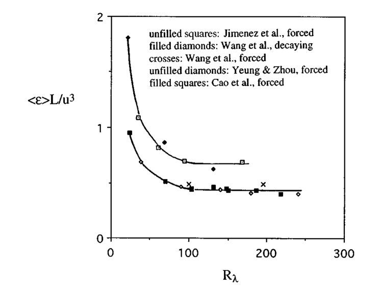
(a) [Sreenivasan [184]]: The variation of the quantity $\varepsilon^{\nu}LU^{-3}$ with the Taylor microscale Reynolds number $\mathrm{Re\,}_{\lambda}$ in simulations of homogeneous and isotropic turbulence in periodic box.

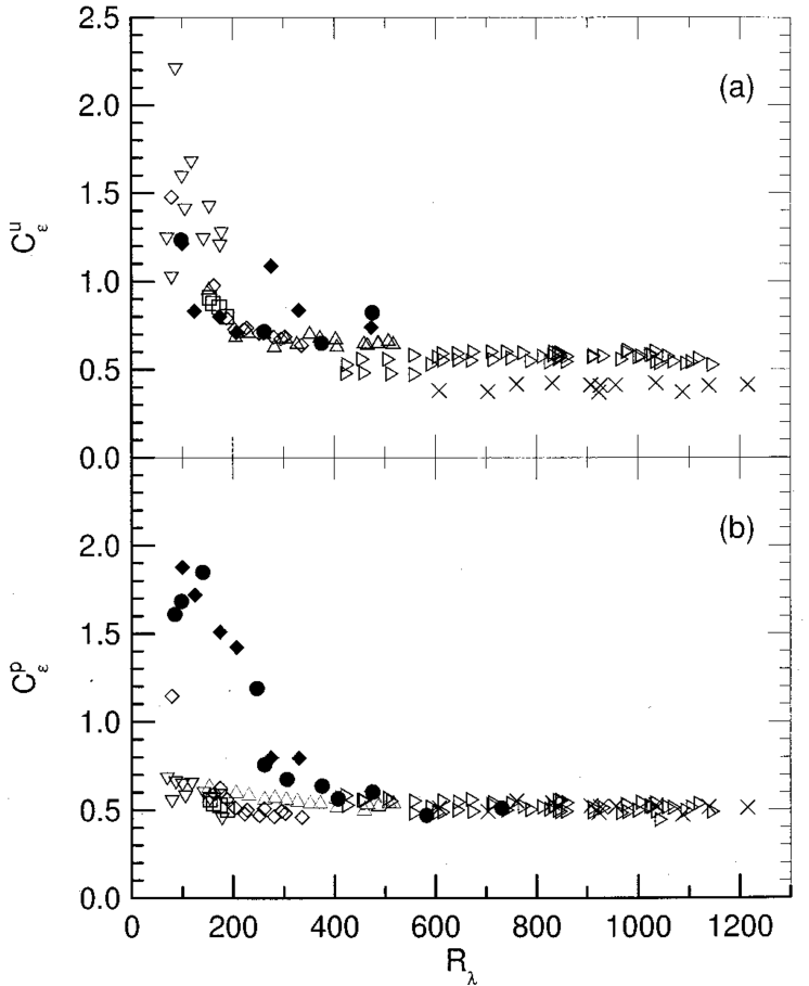
(b) [Pearson, Krogstad, de Water [160]]: $C^{u}_{\varepsilon}=\varepsilon^{\nu}L_{u}U^{-3}$, with $L_{u}=$ streamwise integral length scale; and $C^{p}_{\varepsilon}=\varepsilon^{\nu}L_{p}U^{-3}$, with $L_{p}=$ inverse wavenumber at which peak in energy spectrum occurs.

Figure 1: Experimental and numerical evidence for the anomalous dissipation of energy.

2.2 Basics of the Kolmogorov (’41) theory

Based on the anomalous dissipation of energy and certain scaling arguments, in 1941 Kolmogorov [115, 116, 114] proposed a theory for homogenous isotropic turbulence, whose key predictions we summarize below. We follow the presentation in [81, 150, 71, 180], to which we refer the reader for further details.

Besides the zeroth law of turbulence (2.8), the assumptions of Kolmogorov’s theory are homogeneity, isotropy, and self-similarity. Let $\widehat{z}\in{\mathbb{S}}^{2}$ be a unit direction vector and let $\ell>0$ be a length scale in the inertial range, meaning that $\ell_{D}\ll\ell\ll\ell_{I}$, where $\ell_{I}$ is the integral scale of the system (the inverse of the maximal Fourier frequency $\kappa_{I}$ active in the force), and $\ell_{D}=\nu^{\nicefrac{{3}}{{4}}}\varepsilon^{-\nicefrac{{1}}{{4}}}$ is the Kolmogorov dissipative length scale (the only object which has the physical unit of $L$ and may be written as $\nu^{a}\varepsilon^{b}$; recall that $\nu$ has units of $LU$). Recall the notation (2.5) for velocity increments. Homogeneity is the assumption that the statistics of turbulent flows is shift invariant: at large Reynolds numbers the velocity increment $\delta v^{\nu}(x,t;\ell\widehat{z})$ has the same probability distribution for every $x\in\mathbb{T}^{3}$. Isotropy is the assumption that the statistics of turbulent flows is locally rotationally invariant: the probability distribution for $\delta v^{\nu}(x,t;\ell\widehat{z})$ is the same for all $\widehat{z}\in{\mathbb{S}}^{2}$. Lastly, self-similarity postulates the existence of an exponent $h>0$, such that $\delta v^{\nu}(x,t;\lambda\ell\widehat{z})$ and $\lambda^{h}\delta v^{\nu}(x,t;\ell\widehat{z})$ have the same law, for $\lambda>0$ such that both $\ell$ and $\lambda\ell$ lie in the inertial range. Based on these assumptions, the theory makes predictions about structure functions and the energy spectrum.

For $p\geq 1$ one may define the $p^{th}$ order longitudinal structure function

$$S_{p}^{\|}(\ell)=\left\langle(\delta v^{\nu}(x,t;\ell\widehat{z})\cdot\widehat{z})^{p}\right\rangle$$

where the ensemble/long-time $\left\langle\cdot\right\rangle$ takes into account homogeneity and isotropy, so that we do not have to explicitly write averages in $x$ over $\mathbb{T}^{3}$ and in $\widehat{z}$ over ${\mathbb{S}}^{2}$. Note that for $p$ which is odd, $S_{p}^{\|}(\ell)$ need not a-priori have a sign. Instead, one may define the $p^{th}$ order absolute structure function

$$S_{p}(\ell)=\left\langle|\delta v^{\nu}(x,t;\ell\widehat{z})|^{p}\right\rangle$$

which is intimately related to the definition of a Besov space. $S_{p}(\ell)$ scales in the same way as $S_{p}^{\|}(\ell)$, and they both have physical units of $U^{p}$. Notice that since $\varepsilon\ell$ has units of $U^{3}$, it follows that $(\varepsilon\ell)^{\nicefrac{{p}}{{3}}}$ has the same physical units as $S_{p}(\ell)$. Consequently, the only the value of the self-similarity exponent which is consistent with physical units as $\ell\to 0$ is $h=\nicefrac{{1}}{{3}}$, and thus the Kolmogorov theory predicts the asymptotic behavior

$$S_{p}(\ell)\sim(\varepsilon\ell)^{\nicefrac{{p}}{{3}}}$$ (2.9)

for $\ell$ in the inertial range, in the infinite Reynolds number limit. Denoting by $\zeta_{p}$ the limiting structure function exponent

$$\zeta_{p}=\lim_{\ell\to 0}\lim_{\nu\to 0}\frac{\log\left(S_{p}(\ell)\right)}{\log\left(\varepsilon\ell\right)}\,,$$ (2.10)

the relation (2.9) indicates that in Kolmogorov’s theory of homogenous isotropic turbulence we have

$$\zeta_{p}=\frac{p}{3}\,,\qquad\mbox{for all}\qquad p\geq 1\,,$$ (2.11)

in view of the assumption of self-similarity of the statistics at small scales. Figure 2 shows that this heuristic argument for the value of $\zeta_{p}$ yields a surprisingly small deviations, at least for $p$ close to $3$.

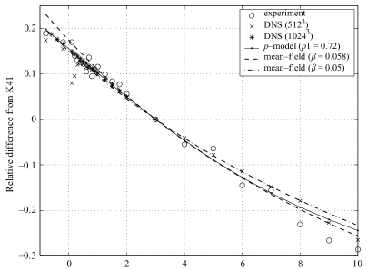
Figure 2: Mild deviations of $\zeta_{p}$ from $p/3$. [Chen, Dhruva, Kurien, Sreenivasan, Taylor [23]]. The graphic plots $p$ versus $(\zeta_{|p|}-\frac{p}{3})\frac{3}{p}$ for various nonzero moments $p$, as gathered from experiments (circles) and direct numerical simulations (crosses and stars). The solid line is the outcome of the $p$-model of [Meneveau-Sreenivasan [144]]. The dashed and dotted lines are predictions of the $\beta$ model of [Yakhot [204]].

Nonetheless, as seen in Figure 2, except for $p=3$, when the Kolmogorov prediction $\zeta_{3}=1$ is indeed supported by all the experimental evidence, for $p\neq 3$ experiments do indeed deviate from the Kolmogorov prediction. This is related to the phenomenon of intermittency discussed in Section 2.4 below.

For the third order longitudinal structure function $S_{3}^{\|}$, Kolmogorov derived what is considered an exact result in turbulence, the famous $4/5$-law, which states that

$$S_{3}^{\|}(\ell)\sim-\frac{4}{5}\varepsilon\ell$$ (2.12)

holds in the infinite Reynolds number limit, for $\ell\ll\ell_{I}$. Identity (2.12) is remarkable because a-priori, there is no good reason for the cubic power of the longitudinal increments to have a sign, on average. Moreover, in addition to claiming that $\zeta_{3}=1$, (2.12) predicts the universal pre-factor of $-\nicefrac{{4}}{{5}}$. Compelling experimental support of the $4/5$-law is provided for instance by the measurement in Figure 3.

Figure 3: Experimental evidence for $S_{3}^{\|}(\ell)=-\frac{4}{5}(\varepsilon\ell)$. The quantity $-S_{3}^{\|}(\ell)/(\varepsilon\ell)$ is plotted as a function of $\ell$. Squares denote experimental observations of centerline in pipe flow at $\mathrm{Re\,}=230000$. Circles indicate data from a $512^{3}$ DNS of homogenous turbulence at $\mathrm{Re\,}=220$. Dots indicate the $4/5$ law. [K. R. Sreenivasan et. al. [185]]

From a mathematical perspective the $4/5$-law is particularly intriguing because under quite mild assumptions one may establish it rigorously. We refer the reader to the results and excellent discussions in [154, 68], where evidence is provided that in the inviscid limit, i.e. for the Euler equations, the (2.12) should hold with just local space-time averaging in $(x,t)$ and angular averaging over the direction of the separation vector $\widehat{z}$ (without the assumption of isotropy). This viewpoint is intimately related to Onsager’s predictions discussed in Section 2.3 below.

For $p=2$, from (2.9)–(2.11) the Kolmogorov prediction yields $\zeta_{2}=\nicefrac{{2}}{{3}}$. One may translate this scaling of the second order structure function into the famous $-\nicefrac{{5}}{{3}}$ energy density spectrum, defined in terms of Fourier projection operators as follows. For $\kappa>0$ the mean kinetic energy per unit mass carried by wavenumber $\leq\kappa$ in absolute value is given by $\frac{1}{2}\left\langle|\mathbb{P}_{\leq\kappa}v^{\nu}|^{2}\right\rangle$. The energy spectrum is then defined as

$${\mathcal{E}}(\kappa)=\frac{1}{2}\frac{d}{d\kappa}\left\langle|\mathbb{P}_{\leq\kappa}v^{\nu}|^{2}\right\rangle$$ (2.13)

so that the total kinetic energy may be written as $\frac{1}{2}\left\langle|v^{\nu}|^{2}\right\rangle=\int_{0}^{\infty}{\mathcal{E}}(\kappa)d\kappa$. The Kolmogorov prediction $\zeta_{2}=\nicefrac{{2}}{{3}}$ then translates into

$${\mathcal{E}}(\kappa)\sim\epsilon^{2/3}\kappa^{-5/3},$$ (2.14)

for $\kappa^{-1}$ in the inertial range, and in the infinite Reynolds number limit. See [81] for experimental support for (2.14). This power law requires however that velocity fluctuations are uniformly distributed over the three dimensional domain, which as discussed in Section 2.4 below, is not always justified (see Figure 5).

2.3 Basics of the Onsager (’49) theory

In his famous paper on statistical hydrodynamics, Onsager [157] considered the possibility that “turbulent energy dissipation […] could take place just as readily without the final assistance of viscosity […] because the velocity field does not remain differentiable”. The pointwise energy balance for smooth solutions $v$ of the Euler equations (1.2) is

$$\partial_{t}\frac{|v|^{2}}{2}+\nabla\cdot\left(v\left(\frac{|v|^{2}}{2}+p\right)\right)=f\cdot v\ .$$ (2.15)

Integrating over the periodic domain we obtain the kinetic energy balance

$$\frac{d}{dt}\fint_{\mathbb{T}^{3}}\frac{|v|^{2}}{2}dx=\fint_{\mathbb{T}^{3}}f\cdot vdx\,,$$ (2.16)

which becomes a conservation law when $f\equiv 0$. Onsager is referring to the fact that if the solution $v$ of (1.2) is not sufficiently smooth, i.e. it is a weak solution, then the energy balance/conservation (2.16) cannot be justified. Onsager’s remarkable analysis went further and made a precise statement about the necessary regularity of $v$ which is required in order to justify (2.16). This has been phrased in mathematical terms as the Onsager Conjecture (see Conjecture 3.2 below). We refer to the review articles [71, 180, 69] for a detailed account of the Onsager theory of ideal turbulence, and present here only some of the ideas (in terms of Fourier projection operators, as in Onsager’s work [157]).

We regularize a weak solution $v$ of the Euler equations (1.2), by a smooth cutoff in the Fourier variables at frequencies $\leq\kappa$, and consider the kinetic energy of $\mathbb{P}_{\leq\kappa}v$. Then, similarly to (2.15)–(2.16) we obtain that

$$\frac{d}{dt}\fint_{\mathbb{T}^{3}}\frac{|\mathbb{P}_{\leq\kappa}v|^{2}}{2}dx=\fint_{\mathbb{T}^{3}}\mathbb{P}_{\leq\kappa}f\cdot\mathbb{P}_{\leq\kappa}vdx-\Pi_{\kappa}$$ (2.17)

where as in [157, 70, 35, 81, 24] we denote by $\Pi_{\kappa}$ the mean energy flux through the sphere of radius $\kappa$ in frequency space, i.e.

$$\Pi_{\kappa}=-\fint_{\mathbb{T}^{3}}\mathbb{P}_{\leq\kappa}(v\otimes v)\colon\nabla\mathbb{P}_{\leq\kappa}vdx=\fint_{\mathbb{T}^{3}}\underbrace{\Big{(}(\mathbb{P}_{\leq\kappa}v\otimes\mathbb{P}_{\leq\kappa}v)-\mathbb{P}_{\leq\kappa}(v\otimes v)\Big{)}\colon\nabla\mathbb{P}_{\leq\kappa}v}_{=:\pi_{\kappa}(x,t)}dx\,.$$ (2.18)

The above defined mean energy flux $\Pi_{\kappa}$, and corresponding density $\pi_{\kappa}$ may also be computed as in the right side of (3.1) below, with $\ell\approx\kappa^{-1}$. From (2.17) we deduce upon passing $\kappa\to\infty$ that the energy balance (2.16) is holds if and only if the total energy flux

$$\Pi=\lim_{\kappa\to\infty}\Pi_{\kappa}\,,$$ (2.19)

vanishes. Onsager’s prediction is that in order for $\Pi$ to be nontrivial, and thus for the weak solution $v$ of the Euler equation to be non-conservative, it should not obey $|\delta v(x;z)|\lesssim|z|^{\theta}$ with $\theta>\nicefrac{{1}}{{3}}$ (see Part (a) of Conjecture 3.2 below).

We emphasize that in 3D turbulent flows the energy transfer from one scale/frequency to another is observed to be mainly local, i.e. the principal contributions to $\Pi_{\kappa}$ come from $\mathbb{P}_{\approx\kappa^{\prime}}v$, with $\kappa^{\prime}\approx\kappa$. A rigorous estimate on the locality of the energy transfer arises in [24], where it is proven that

$$|\Pi_{2^{j}}|\lesssim\sum_{i=1}^{\infty}2^{-2/3|j-i|}2^{i}\|\mathbb{P}_{\approx 2^{i}}v\|_{L^{3}}^{3}\,.$$ (2.20)

Estimate (2.20) gives the best known condition on $v$ which ensures $\Pi=0$, namely $v\in L^{3}_{t}B^{\nicefrac{{1}}{{3}}}_{3,c_{0},x}$ (cf. [24]), a condition which is for instance sharp in the case of the 1D Burgers equation [180].

It is not an accident that the $\nicefrac{{1}}{{3}}$-derivative singularities required by Onsager for a dissipative anomaly $\Pi\neq 0$, matches Kolmogorov’s assumed $\nicefrac{{1}}{{3}}$ local self-similarity exponent required for $\varepsilon>0$. As already observed by Onsager [157], if $v$ is a weak solution of the Euler equations which is a strong limit of a sequence $\{v^{\nu}\}$ of Navier-Stokes solutions for which the anomalous dissipation of energy (2.8) holds, then the total energy flux associated to $v$ must match this dissipation anomaly in the vanishing viscosity limit:

$$\varepsilon=\langle\Pi\rangle.$$ (2.21)

On the experimental side, the evidence for (2.21) is quite convincing, see e.g. Figure 4.

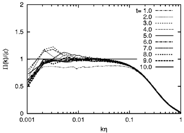
Figure 4: Kolmogorov’s anomalous energy dissipation rate $\varepsilon$ and Onsager’s energy flux $\Pi_{\kappa}$ appear to agree, at least for $\kappa$ in the inertial range. [Kaneda et al [106]]: $2048^{3}$ DNS runs on Earth Simulator computing system.

The energy flux provides a connection between the Kolmogorov and Onsager theories, and a physics derivation of (2.21) is as follows [81]. Assume for simplicity that $f^{\nu}=f$ is statistically stationary, and that $\mathbb{P}_{\kappa_{I}}f=f$ for some integral frequency $\kappa_{I}$. Denote by $\Pi_{\kappa}^{\nu}$ the energy flux through the frequency ball of radius $\kappa$ for a solution $v^{\nu}$ of the Navier-Stokes equation, i.e. replace $v$ in (2.18) with $v^{\nu}$. Then similarly to (2.17), since the ensemble/long-time average $\left\langle\cdot\right\rangle$ is stationary, we obtain that

$$\left\langle\Pi_{\kappa}^{\nu}\right\rangle+\nu\left\langle|\nabla\mathbb{P}_{\leq\kappa}v^{\nu}|^{2}\right\rangle=\left\langle f\cdot\mathbb{P}_{\leq\kappa}v^{\nu}\right\rangle$$ (2.22)

for $\kappa\geq\kappa_{I}$. On the other hand, assuming that the Euler solution is statistically stationary, (2.17) yields

$$\left\langle\Pi_{\kappa}\right\rangle=\left\langle f\cdot\mathbb{P}_{\leq\kappa}v\right\rangle$$ (2.23)

To conclude, we recall that from the definition (2.4) we have $\left\langle D(v^{\nu})\right\rangle=\lim_{\kappa\to\infty}\left\langle\Pi_{\kappa}^{\nu}\right\rangle$ (cf. [60]), and with $\varepsilon^{\nu}$ as given by (2.7), we pass $\kappa\to\infty$ in (2.22) and (2.23), to arrive at

$$\varepsilon-\left\langle\Pi\right\rangle=\lim_{\nu\to 0}\left(\varepsilon^{\nu}-\left\langle\Pi\right\rangle\right)=\lim_{\nu\to 0}\left\langle f\cdot(v^{\nu}-v)\right\rangle=0$$ (2.24)

since we assumed $v^{\nu}\to v$. Note that here we have made a number of assumptions which are not justified.

2.4 Intermittency

In this last part of Section 2 we consider the intermittent nature of turbulent flows. This is a topic of significant debate [117, 142, 83, 82, 183, 145, 176, 204]. Large parts of the books [81, 150] are dedicated to this mystery, and we refer to these texts, and to the recent papers [87, 26] for a more detailed discussion. Our interest stems from the fact that this phenomenon is the primary motivation for the intermittent convex integration scheme discussed in Section 7.

In a broad sense, intermittency is characterized as a deviation from the Kolmogorov 1941 laws. Already in 1942 Landau remarked that the rate of energy dissipation in a fully developed turbulent flow is observed to be spatially and temporally inhomogeneous, and thus Kolmogorov’s homogeneity and isotropy assumptions need not be valid (cf. [125, 81]). Figure 5 shows a typical signal used in experiments to measure $\varepsilon^{\nu}$. The main feature seems to be the presence of sporadic dramatic events, during which there are large excursions away from the average.

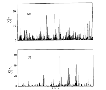
Figure 5: [Meneveau & Sreenivasan [145]]. Two typical signals, with $\varepsilon^{\prime}=(du_{1}/dt)^{2}$, serving as the surrogate of the energy dissipation rate, are plotted here upon normalizing by their mean values. Graph (a) was in a laboratory boundary layer at a moderate Reynolds number. Graph (b) was obtained in the atmospheric surface layer at high Reynolds number ($10^{4}$). The increased intermittency at the higher Reynolds number is clear.

A common signature of intermittency is that the structure function exponents $\zeta_{p}$ deviate from the Kolmogorov predicted value of $\nicefrac{{p}}{{3}}$, and moreover, for $p\neq 3$ they do not appear to be universal. Figure 6, compiled by Frisch in [81], highlights this fact. We again see in Figure 6 that the prediction $\zeta_{3}=1$ seems to be confirmed by all experimental data, but for $p>3$ we have $\zeta_{p}<\nicefrac{{p}}{{3}}$, while for $p<3$ we have $\zeta_{p}>\nicefrac{{p}}{{3}}$.

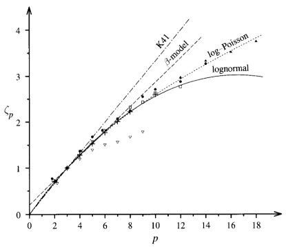
Figure 6: [Frisch [81]]: Anomalous scaling of structure functions. Data: inverted white triangles: [Van Atta-Park [195]]; black circles, white squares, black triangles: [Anselmet, Gagne, Hopfinger, Antonia [1]] at $\mathrm{Re\,}=515,536,852$; $+$ signs: from S1 ONERA wind tunnel.

While there are many phenomenological theories for predicting the structure function exponents $\zeta_{p}$ in intermittent turbulent flows, none of them seem to be able to explain all experimental data, and their connection to dynamical evolution of the underlying Navier-Stokes/Euler equations seems to be limited.

A particularly appealing intermittency model is the $\beta$-model of Frisch-Sulem-Nelkin [83], which was revisited recently by Cheskidov-Shvydkoy [26] from a modern analysis perspective. In order to make a connection with the measure-theoretic support of the defect measure $D(v)$, the authors in [26] define active regions $A_{q}$ whose volumes $V_{q}$ are given in terms of an $L^{2}-L^{3}$ skewness factor which measures the saturation of the Bernstein inequalities at frequencies $\approx 2^{q}$. More precisely, using the active volumes defined as

$$V_{q}=L^{3}\frac{\left\langle|\mathbb{P}_{\approx 2^{q}}v|^{2}\right\rangle^{3}}{\left\langle|\mathbb{P}_{\approx 2^{q}}v|^{3}\right\rangle^{2}},$$

the intermittency dimension $D$ is defined as

$$D=3-\liminf_{q\to\infty}\frac{\log_{2}(L^{3}V_{q}^{-1})}{q},$$

and then the $\beta$-model yields corrections [83, 81, 26] to the Kolmogorov predictions (2.11) and (2.14) as

$$\zeta_{p}=\frac{p}{3}+(3-D)\left(1-\frac{p}{3}\right)\qquad\mbox{and}\qquad{\mathcal{E}}(\kappa)\sim\varepsilon^{-\nicefrac{{2}}{{3}}}\kappa^{-\nicefrac{{5}}{{3}}}\left(\frac{\kappa_{I}}{\kappa}\right)^{1-\nicefrac{{D}}{{3}}}.$$

Note that the Kolmogorov theory corresponds to $D=3$, in which the turbulent events fill space. On the other hand, the simulation of [106] estimates $D\approx 2.7$.

We note in closing that in the intermittent convex integration construction of Section 7, it is essential that the building blocks concentrate on a set with dimension strictly less than one. This translates (cf. estimate (7.27)) into the fact that the skewness ratio of our intermittent building blocks $\frac{\left\|\cdot\right\|_{L^{1}}}{\left\|\cdot\right\|_{L^{2}}}$ scales better than the frequency of the building blocks to the power $-1$. This is one of the essential aspects of the construction, and is discussed in detail in Sections 4 and 7.

3 Mathematical results

3.1 The Euler Equations

Local well-posedness for smooth solutions to the Euler equations is classical [130] (cf. [141]). By the Beale-Kato-Majda criterion, global well-posedness for the Euler equations is known to hold under the assumption that the $L^{\infty}$ norm of the vorticity is $L^{1}$ integrable in time [7]. In 2D, vorticity is transported, leading to global well-posedness of smooth solutions [96, 203] as well as weak solutions with $L^{\infty}$ bounded vorticity [205, 141, 198]. Global well-posedness for smooth solutions to the 3D Euler equation is famously unresolved, and is intimately related to the Clay Millennium problem [74]. Indeed, there exists numerical evidence to suggest that the 3D Euler equations may develop a singularity [137, 136] (cf. [162, 88, 89, 30]). Recently, Elgindi and Jeong demonstrated the formation of a singularity in the presence of a conical hourglass-like boundary [62].

Within the class of weak solutions, the Euler equations are known to display paradoxical behavior. In the seminal work [173], Scheffer demonstrated the existence of non-trivial weak solutions with compact support in time (cf. [178, 179]). These results represent a quite drastic demonstration of non-uniqueness for weak solutions to the Euler equations. For the purpose of this article, we define a weak solution for (1.2) as:

Definition 3.1.

A vector field $v\in C^{0}_{t}L^{2}_{x}$ is called a weak solution of the Euler equations if for any $t$ the vector field $v(\cdot,t)$ is weakly divergence free, has zero mean, and satisfies the Euler equation distributionally:

$$\int_{\mathbb{R}}\!\int_{\mathbb{T}^{3}}v\cdot(\partial_{t}\varphi+(v\cdot\nabla)\varphi)dxdt=0\,,$$

for any divergence free test function $\varphi$. For a weak solution to the Cauchy problem this definition is modified in the usual way.

As mentioned in Section 2, one motivation for studying weak solutions to the Euler equations, is that in the inviscid limit, turbulent solutions exhibiting a dissipation anomaly are necessarily weak solutions. In [157] Onsager conjectured the following dichotomy:

Conjecture 3.2 (Onsager’s conjecture).

1. Any weak solution $v$ belonging to the Hölder space $C^{\theta}_{x,t}$ for $\theta>\nicefrac{{1}}{{3}}$ conserves kinetic energy.

2. For any $\theta<\nicefrac{{1}}{{3}}$ there exist weak solutions $v\in C^{\theta}_{x,t}$ which dissipate kinetic energy.

Part (a) of this conjecture was partially established by Eyink in [70], and later proven in full by Constantin, E and Titi in [35] (see also [60, 24], and the more recent work [182], for refinements). The proof follows by a simple commutator argument: Suppose $v$ is a weak solution to the Euler equations, and let $v_{\ell}$ be the spatial mollification of $v$ a length scale $\ell$. Then, $v_{\ell}$ satisfies

$$\int_{\mathbb{T}^{3}}\left|v_{\ell}(x,t)\right|^{2}dx-\int_{\mathbb{T}^{3}}\left|v_{\ell}(x,0)\right|^{2}dx=2\int_{0}^{t}\int_{\mathbb{T}^{3}}\mathrm{tr\,}((v\otimes v)_{\ell}(\nabla v_{\ell}))dxds~{}.$$

Applying the identity

$$\int_{\mathbb{T}^{3}}\mathrm{tr\,}((v_{\ell}\otimes v_{\ell})(\nabla v_{\ell}))dx\equiv 0~{},$$

yields

$$\int_{\mathbb{T}^{3}}\left|v_{\ell}(x,t)\right|^{2}dx-\int_{\mathbb{T}^{3}}\left|v_{\ell}(x,0)\right|^{2}dx=2\int_{0}^{t}\int_{\mathbb{T}^{3}}\mathrm{tr\,}\left(((v\otimes v)_{\ell}-(v_{\ell}\otimes v_{\ell}))(\nabla v_{\ell})\right)dxd\tau\,.$$ (3.1)

Applying the commutator estimate Proposition 6.5, in Section 5, we deduce

$$\left|\int_{\mathbb{T}^{3}}\left|v_{\ell}(x,t)\right|^{2}dx-\int_{\mathbb{T}^{3}}\left|v_{\ell}(x,0)\right|^{2}dx\right|\leq C\ell^{3\theta-1}\left\|v\right\|_{C^{\theta}}^{3}~{}.$$

Thus, if $\theta>\nicefrac{{1}}{{3}}$, the right hand side converges to zero as $\ell\rightarrow 0$.

Concerning part (b) of the Onsager conjecture, strictly speaking the weak solutions of Scheffer are not dissipative, as dissipative solutions are required to have non-increasing energy. The existence of dissipative weak solutions to the Euler equations was first proven by Shnirelman in [179] (cf. [45, 46]). In the groundbreaking papers [48, 49], De Lellis and Székelyhidi Jr. made significant progress towards Part (b) of Onsager’s conjecture by proving the first construction of dissipative Hölder continuous weak solutions to the Euler equations (see Theorem 5.1). After a series of advancements [98, 16, 14, 17, 44], part (b) of the Onsager conjecture was resolved by Isett in [102]:

Theorem 3.3 (Theorem 1, [102]).

For any $\beta\in(0,\nicefrac{{1}}{{3}})$ there exists a nonzero weak solution $v\in C^{\beta}(\mathbb{T}^{3}\times\mathbb{R})$, such that $v$ vanishes identically outside of a finite interval.

Like the original paper of Scheffer [173], the weak solutions constructed by Isett [102] are not strictly dissipative. This technical issue was resolved in the paper [18], in which the precise statement of part (b) was proven:

Theorem 3.4 (Theorem 1.1, [18]).

Let $e\colon[0,T]\to\mathbb{R}$ be a strictly positive smooth function. For any $\beta\in(0,\nicefrac{{1}}{{3}})$ there exists a weak solution $v\in C^{\beta}(\mathbb{T}^{3}\times[0,T])$ of the Euler equations (1.2), whose kinetic energy at time $t\in[0,T]$ equals $e(t)$.

The exponent $\nicefrac{{1}}{{3}}$ in Onsager’s conjecture can be viewed in terms of a larger class of threshold exponents at which a dichotomy in the behavior of solutions arises. In a recent expository paper [112] on the work of Nash, Klainerman considered various threshold exponents in the context of non-linear PDE (see also [19] for a discussion of thresholds exponents in the context of hydrodynamic equations). In order to simply the discussion, consider Banach spaces of the form $X^{\alpha}=C_{t}^{0}C^{\alpha}_{x}$. As in [112, Page 11], let us define the following exponents:

• The scaling exponent $\alpha_{*}$ determines the norm for which the $X^{\alpha_{*}}$ is invariant under the natural scalings of the equation.

• The Onsager exponent $\alpha_{O}$ determines the norm for which the Hamiltonian of a PDE is conserved.

• The Nash exponent $\alpha_{N}$ determines the threshold for which the PDE is flexible or rigid in the sense of the $h$-principle.

• The uniqueness exponent $\alpha_{U}$ determines the threshold for which uniqueness of solutions holds.

• The well-posedness exponent $\alpha_{WP}$ determines the threshold for which local well-posedness holds.

Since flexibility implies non-uniqueness, and well-posedness implies uniqueness, we have $\alpha_{N}\leq\alpha_{U}\leq\alpha_{WP}$. For the Euler equations, $\alpha_{WP}=1$ (cf. [96, 4, 10, 63]), $\alpha_{U}$ is conjectured to be $1$ (the Beale-Kato-Majda criterion implies that $\alpha_{U}\leq 1$), $\alpha_{O}=1/3$ (cf. [35, 24, 102, 18]), and $\alpha_{*}=0$. In general, one expects the ordering $\alpha_{*}\leq\alpha_{O}\leq\alpha_{N}\leq\alpha_{U}\leq\alpha_{WP}$ (cf. [112, Equation (0.7)]).

3.2 The Navier-Stokes Equations

The global well-posedness for the 3D Navier-Stokes equations, is one of the most famous open problems in mathematics, subject to one of seven Clay Millennium Prize problems [74]. Local well-posedness in various scale invariant spaces follows by classical contraction mapping arguments [84, 109, 113, 127] and global well-posedness typically follows when the datum is small in these spaces. If one relaxes one’s notion of solutions and considers instead weak solutions, then Leray [128] and later Hopf [97] proved that for any finite energy initial datum there exists a global weak solution to the Navier-Stokes equation. More precisely, Leray proved the global existence in the following class of weak solutions:

Definition 3.5.

A vector field $v\in C^{0}_{\rm weak}([0,\infty);L^{2}(\mathbb{T}^{3}))\cap L^{2}([0,\infty);\dot{H}^{1}(\mathbb{T}^{3}))$ is called a Leray-Hopf weak solution of the Navier-Stokes equations if for any $t\in\mathbb{R}$ the vector field $v(\cdot,t)$ is weakly divergence free, has zero mean, satisfies the Navier-Stokes equations distributionally:

$$\int_{\mathbb{R}}\!\int_{\mathbb{T}^{3}}v\cdot(\partial_{t}\varphi+(v\cdot\nabla)\varphi+\nu\Delta\varphi)dxdt+\int_{\mathbb{T}^{3}}v(\cdot,0)\cdot\varphi(\cdot,0)dx=0\,,$$

for any divergence free test function $\varphi$, and satisfies the energy inequality:

$$\frac{1}{2}\int_{\mathbb{T}^{3}}\left|v(x,t)\right|^{2}\,dx+\int_{\mathbb{T}^{3}\times[0,t]}\left|\nabla v(x,s)\right|^{2}\,dxds\leq\frac{1}{2}\int_{\mathbb{T}^{3}}\left|v(x,0)\right|^{2}\,dx\,.$$ (3.2)

Leray-Hopf solutions are known to be regular and unique under the additional assumption that one of the Ladyženskaja-Prodi-Serrin conditions are satisfied, i.e. the solution is bounded in a scaling invariant space $L^{p}_{t}L^{q}_{x}$ for $\nicefrac{{2}}{{p}}+\nicefrac{{3}}{{q}}=1$ [111, 161, 175, 104]. One possible strategy to proving that the Navier-Stokes equation is well-posed is then to show that the weak solutions are smooth [74]. Since smooth solutions are necessarily unique, such a result would imply the uniqueness of weak solutions.

In recent work by the authors [20], another class of weak solutions was considered, namely:

Definition 3.6.

A vector field $v\in C^{0}_{t}L^{2}_{x}$ is called a weak solution of the Navier-Stokes equations if for any $t$ the vector field $v(\cdot,t)$ is weakly divergence free, has zero mean, and

$$\int_{\mathbb{R}}\!\int_{\mathbb{T}^{3}}v\cdot(\partial_{t}\varphi+(v\cdot\nabla)\varphi+\nu\Delta\varphi)dxdt=0\,,$$

for any divergence free test function $\varphi$.

The above class is weaker than Definition 3.5 in the sense that solutions need not satisfy the energy inequality (3.2); however, they are stronger in the sense that the $L^{2}$ norm in space is required to be strongly continuous in time. Such solutions satisfy the integral equation [72]

$$v(\cdot,t)=e^{\nu\Delta t}v(\cdot,0)+\int_{0}^{t}e^{\nu\Delta(t-s)}\mathbb{P}\mathrm{div\,}(v(\cdot,s)\otimes v(\cdot,s))ds\,,$$

and are sometimes called mild or Oseen solutions (cf. [127, Definition 6.5]). As is the case for Leray-Hopf solutions, weak solutions of the form described in Definition 3.6 are known to be regular under the additional assumption that one of Ladyženskaja-Prodi-Serrin conditions is satisfied [72, 85, 135, 126, 119, 86]. The principal result of [20] is:

Theorem 3.7 (Theorem 1.2, [20]).

There exists $\beta>0$, such that the following holds. For any nonnegative smooth function $e(t)\colon[0,T]\to[0,\infty)$, and any $\nu\in(0,1]$, there exists a weak solution of the Navier-Stokes equations $v\in C^{0}([0,T];H^{\beta}(\mathbb{T}^{3}))\cap C^{0}([0,T];W^{1,1+\beta}(\mathbb{T}^{3}))$, such that $\int_{\mathbb{T}^{3}}|v(x,t)|^{2}dx=e(t)$ holds for all $t\in[0,T]$.

Since the energy profile may be chosen to have compact support, and $v\equiv 0$ is a solution, the result implies the non-uniqueness of weak solutions to the Navier-Stokes equations, in the sense of Definition 3.6. Theorem 3.7 represents a failure of the strategy of proving global well-poseness via weak solutions, at least for the class of weak solutions defined in Definition 3.6.

One may naturally ask if such non-uniqueness holds for Leray-Hopf weak solutions. This problem remains open. Non-uniqueness of Leray-Hopf solutions were famously conjectured by Ladyženskaja [123]. More recently, Šverák and Jia proved the non-uniqueness of Leray-Hopf weak solutions assuming that a certain spectral assumption holds [105]. While Guillod and Šverák have provided in [93] compelling numerical evidence that the assumption of [105] may be satisfied, a rigorous proof remains to date elusive.

An alternate, stronger version of Leray-Hopf solutions is often considered in the literature:

Definition 3.8.

A Leray-Hopf weak solution to the Navier-Stokes equation satisfying the local energy equality, is a vector field satisfying the same conditions as detailed in Definition 3.5; however, with the energy equality (3.2) replaced with the local energy inequality

$$\frac{1}{2}\int_{\mathbb{T}^{3}}\left|v(x,t)\right|^{2}\,dx+\int_{\mathbb{T}^{3}\times[t_{0},t]}\left|\nabla v(x,s)\right|^{2}\,dxds\leq\frac{1}{2}\int_{\mathbb{T}^{3}}\left|v(x,t_{0})\right|^{2}\,dx\,.$$ (3.3)

for almost every $t_{0}\geq 0$ and all $t>t_{0}$.

The advantage of Definition 3.8 over Definition 3.5 is that from the localized energy inequality (3.3), one can deduce that the solutions possess epochs of regularity, i.e. many time intervals on which they are smooth. Indeed, in [128], Leray proved that such solutions are almost everywhere in time smooth since the singular set of times $\Sigma_{T}$ has Hausdorff dimension $\leq\nicefrac{{1}}{{2}}$. Improving on this, Scheffer [168] proved that the $\nicefrac{{1}}{{2}}$-dimensional Hausdorff measure of $\Sigma_{T}$ is $0$. More detailed results, concerning the Minkowski dimension have been obtained in [167, 121].

A curious consequence of the partial regularity result of Leray [128], the local-wellposedness theory and the weak-strong uniqueness result of Prodi-Serrin [161, 175, 127, 202], is that if a Leray-Hopf solution in the sense of Definition 3.8 is not smooth for some time $t>0$, then on an open interval in time the solution would be in fact a strong solution that blows up, implying a negative answer to Millennium prize question. Thus assuming for the moment that the Millennium prize question is out of reach, one is left to prove the non-uniqueness result of Leray-Hopf solutions in the sense of Definition 3.8 via a bifurcation at $t=0$ – this is indeed the strategy employed by Šverák and Jia [105]. Unfortunately, this suggests that convex integration is perhaps ill-suited for the task of proving non-uniqueness of Leray-Hopf solutions in the sense of Definition 3.8. However, the above argument does not apply in the context of the Leray-Hopf solutions defined in Definition 3.5, and thus the argument does not rule out a proof of non-uniqueness of such solutions via the method of convex integration.

The partial regularity theory for Leray-Hopf solutions leads to the natural question of whether there exists weak, singular solutions to the Navier-Stokes equations that are smooth outside a suitably small set in time. In [15], jointly with M. Colombo, the following result was established:

Theorem 3.9 (Theorem 1.1, [15]).

There exists $\beta>0$ such that the following holds. For $T>0$, let $u^{(1)},u^{(2)}\in C^{0}([0,T];\dot{H^{3}}(\mathbb{T}^{3}))$ be two strong solutions of the Navier-Stokes equations. There exists a weak solution $v\in C([0,T];H^{\beta}(\mathbb{T}^{3}))$ and is such that

$$v(t)=u^{(1)}(t)~{}for~{}t\in[0,\nicefrac{{T}}{{3}}]\quad\mbox{and}\quad v(t)\ =u^{(2)}(t)~{}for~{}~{}t\in[\nicefrac{{2T}}{{3}},T]$$

Moreover, there exists a zero Lebesgue measure set of times $\Sigma_{T}\subset(0,T]$ with Hausdorff dimension less than $1-\beta$, such that $v\in C^{\infty}((0,T)\setminus\Sigma_{T}\times\mathbb{T}^{3})$.

Theorem 3.9 represents the first example of a mild/weak solution to the Navier-Stokes equation whose singular set of times $\Sigma_{T}\subset(0,T]$ is both nonempty, and has Hausdorff dimension strictly less than $1$.

In additional to localizing the energy inequality in time, as was done in (3.3), one can also localize it in space, leading to the generalized energy inequality of Scheffer [169]:

$$2\iint\left|\nabla v\right|^{2}\varphi\,dxdt\leq\iint\left(\left|v\right|^{2}(\varphi_{t}+\Delta\varphi)+(\left|v\right|^{2}+2p)v\cdot\nabla\varphi\right)\,dxdt$$ (3.4)

for any non-negative test function $\varphi$. Weak solutions satisfying the generalized energy inequality are known as suitable weak solutions [169, 21]. Note that (3.4) is a restatement of the condition that the defect measure $D[v]$ in (2.3) is non-negative. Following the pioneering work of Scheffer [169, 170], Cafferelli, Kohn and Nirenberg famously proved that the singular set of suitable weak solutions has zero parabolic 1D Hausdorff measure. Analogously to the case of Leray-Hopf solutions in the sense of Definition 3.8, convex integration methods seem ill-suited for proving the non-uniqueness of suitable weak solutions to the Navier-Stokes equation.

In view of the discussion of Section 2, we are led to consider the question of whether the nonconservative weak solutions to the Euler equations obtained in [102, 18] arise as vanishing viscosity limits of weak solutions to the Navier-Stokes equations. In this direction, as a direct consequence of the proof of Theorem 3.7, one obtains:

Theorem 3.10 (Theorem 1.3, [20]).

For $\bar{\beta}>0$ let $v\in C^{\bar{\beta}}_{t,x}(\mathbb{T}^{3}\times[-2T,2T])$ be a zero-mean weak solution of the Euler equations. Then there exists $\beta>0$, a sequence $\nu_{n}\to 0$, and a uniformly bounded sequence $v^{(\nu_{n})}\in C^{0}_{t}([0,T];H^{\beta}_{x}(\mathbb{T}^{3}))$ of weak solutions to the Navier-Stokes equations in the sense of Definition 3.6, with $v^{(\nu_{n})}\to v$ strongly in $C^{0}_{t}([0,T];L^{2}_{x}(\mathbb{T}^{3}))$.

The above result shows that being a strong $L^{2}$ limit of weak solutions to the Navier-Stokes equations, in the sense of Definition 3.6, cannot serve as a selection criterion for weak solutions of the Euler equation. See also Remark 6.4 below.

Lastly, in relation to the threshold exponents considered in Section 3.1, if one considers the family of Banach spaces $C_{t}H^{\alpha}_{x}$, then $\alpha_{*}=\alpha_{WP}=\nicefrac{{1}}{{2}}$ [84, 109, 113, 127, 11]. If we relabel $\alpha_{O}$ the exponent in which the energy equality holds, then as a consequence of Theorem 3.7, and the simple observation that regular solutions obey the energy equality, $0<\alpha_{O},\alpha_{N}\leq\nicefrac{{1}}{{2}}$. As a consequence of the expected ordering $\alpha_{*}\leq\alpha_{O}\leq\alpha_{N}\leq\alpha_{U}\leq\alpha_{WP}$, one would naturally conjecture that $\alpha_{*}=\alpha_{O}=\alpha_{N}=\alpha_{U}=\alpha_{WP}=\nicefrac{{1}}{{2}}$.

4 Convex integration schemes in incompressible fluids

The method of convex integration can be traced back to the work of Nash, who used it to construct exotic counter-examples to the $C^{1}$ isometric embedding problem [152] – a result that was cited in awarding Nash the Abel prize in 2015 (cf. [118]). The method was later refined by Gromov [92] and it evolved into a general method for solving soft/flexible geometric partial differential equations [64]. In the influential paper [151], Müller and Šverák adapted convex integration to the theory of differential inclusions (cf. [110]), leading to renewed interest in the method as a result of its greatly expanded applicability.

4.1 Convex integration schemes for the Euler equations

Inspired by the work [151, 110], and building on the plane-wave analysis introduced by Tartar [189, 190, 55], De Lellis and Székelyhidi Jr., in [48], applied convex integration in the context of weak $L^{\infty}$ solutions of the Euler equations, yielding an alternative proof of Scheffer’s [173] and Schnirelman’s [179] famous non-uniqueness results. The work [48], has since been extended and adapted by various authors to various problems arising in mathematical physics [46, 41, 181, 201, 27], see the reviews [47, 188, 50, 51] and references therein.

In a first attempt at attacking Onsager’s famous conjecture on energy conservation, De Lellis and Székelyhidi Jr.  in their seminal paper [48] developed a new convex integration scheme, motivated and resembling in part the earlier schemes of Nash and Kuiper [152, 118]. In [48], De Lellis and Székelyhidi Jr. demonstrated the existence of continuous weak solutions $v$ to the Euler equations satisfying a prescribed kinetic energy profile, i.e. given a smooth function $e:[0,T]\rightarrow\mathbb{R}^{+}$, there exists a weak solution $v$ such that

$$\frac{1}{2}\int_{\mathbb{T}^{3}}\left|v(t,x)\right|^{2}\,dx=e(t)\,.$$ (4.1)

See Theorem 5.1 below. The proof proceeds via induction. At each step $q\in\mathbb{N}$, a pair $(v_{q},\mathring{R}_{q})$ is constructed solving the Euler-Reynolds system

$$\partial_{t}v_{q}+\mathrm{div\,}(v_{q}\otimes v_{q})+\nabla p_{q}=\mathrm{div\,}\mathring{R}_{q}$$ (4.2a)

$$\mathrm{div\,}v_{q}=0\,.$$ (4.2b)

such that as $q\to\infty$ the sequence $\mathring{R}_{q}$ converges uniformly to $0$ and the sequence $v_{q}$ converges uniformly to a weak solution to the Euler equations (1.2) satisfying (4.1).

The Euler-Reynolds (4.2) system arises naturally in the context of computational fluid mechanics. As mentioned in [81], via [124], the concept of eddy viscosity and microscopic to macroscopic stresses may be traced back to the work of Reynolds [164]. Given a solution $v$ to (1.2), let $\bar{v}$ be the velocity obtained through the application of a filter (or averaging operator) that commutes with derivatives, ignoring the unresolved small scales. Then $(\overline{v},R)$ is a solution to $\eqref{e:euler_reynolds}$ for $R=\overline{v\otimes v}-\overline{v}\otimes\overline{v}=\overline{(v-\overline{v})\otimes(v-\overline{v})}$. In this context the $3\times 3$ symmetric tensor $R$ is referred to as the Reynolds stress.

For comparison, the iterates $(v_{q},\mathring{R}_{q})$ constructed via a convex integration scheme are approximately spatial averages of the final solution $v$ at length scales decreasing with $q$. Owing to the analogy to computational fluid mechanics, we refer to the symmetric tensor $\mathring{R}_{q}$ as the Reynolds stress. Without loss of generality, we will also assume $\mathring{R}_{q}$ to be traceless.

At each inductive step, the perturbation $w_{q+1}=v_{q+1}-v_{q}$ is designed such that the new velocity $v_{q+1}$ solves the Euler-Reynolds system

$$\begin{split}\partial_{t}v_{q+1}+\mathrm{div\,}(v_{q+1}\otimes v_{q+1})+\nabla p_{q+1}&=\mathrm{div\,}\mathring{R}_{q+1}\\ \mathrm{div\,}v_{q+1}&=0\,.\end{split}$$

with a smaller Reynolds stress $\mathring{R}_{q+1}$. Using the equation for $v_{q}$ we obtain the following decomposition of $\mathring{R}_{q+1}$:

$$\begin{split}\mathrm{div\,}\mathring{R}_{q+1}&=\mathrm{div\,}(w_{q+1}\otimes w_{q+1}-\mathring{R}_{q})+\nabla(p_{q+1}-p_{q})\\ &\quad+\partial_{t}w_{q+1}+v_{q}\cdot\nabla w_{q+1}\\ &\quad+w_{q+1}\cdot\nabla v_{q}\end{split}\,,$$

which we denote (line-by-line) as the oscillation error, transport error and Nash error respectively. The Reynolds stress $\mathring{R}_{q+1}$ can then be defined by solving the above divergence equation utilizing an $-1$ order linear differential operator $\mathcal{R}\approx\mathrm{div\,}^{-1}$ (see (5.37)).

The perturbation $w_{q+1}=v_{q+1}-v_{q}$ is constructed as a sum of highly oscillatory building blocks. In earlier papers [48, 49, 16, 14, 103, 17], Beltrami waves were used as the building blocks of the convex integration scheme (see Section 5.4 for a discussion). In later papers [44, 102, 18, 101], Mikado waves were employed (see Section 6.4). These building blocks are used in an analogous fashion to the Nash twists and Kuiper corrugations employed in the $C^{1}$ embedding problem [152, 118]. The perturbation $w_{q+1}$ is designed in order to obtain a cancellation between the low frequencies of the quadratic term $\mathrm{div\,}(w_{q+1}\otimes w_{q+1})$ and the old Reynolds stress error $\mathring{R}_{q}$, thereby reducing the size of the oscillation error. Roughly speaking, the principal part of the perturbation, which we label $w_{q+1}^{(p)}$, will be of the form

$$w_{q+1}^{(p)}\sim\sum_{\xi}a_{\xi}(\mathring{R}_{q})W_{\xi}\,,$$ (4.3)

where the $W_{\xi}$ represent the building blocks oscillating at a prescribed high frequency $\lambda_{q+1}$, and the coefficient functions $a_{\xi}$ are chosen such that

$$\sum_{\xi}a_{\xi}^{2}(\mathring{R}_{q})\fint_{\mathbb{T}^{3}}W_{\xi}\mathring{\otimes}W_{\xi}=-\mathring{R}_{q}\,,$$ (4.4)

where $\mathring{\otimes}$ denotes the trace-free part of the tensor product. As we will see in Section 5.5.3, the principal part will need to be modified from the form presented in (4.3) in order to minimize the transport error. This will be achieved by flowing the building blocks $W_{\xi}$ along the flow generated by $v_{q}$ (see Section 5.5.1). Additionally, in order to ensure that $w_{q+1}$ is divergence free, we will need to introduce a divergence free corrector $w_{q+1}^{(c)}$ such that

$$w_{q+1}=w_{q+1}^{(p)}+w_{q+1}^{(c)}\,,$$

is divergence free.

Heuristically, let us assume for the moment that the frequencies scale geometrically, i.e.

$$\lambda_{q}=\lambda^{q}$$

for some large $\lambda\in\mathbb{N}$. In order that to ensure that the inductive scheme converges to a Hölder continuous velocity $v$ with Hölder exponent $\beta>0$, then by a scaling analysis, the perturbation amplitude is required to satisfy the bound

$$\left\|w_{q+1}\right\|_{C^{0}}\leq\lambda_{q+1}^{-\beta}\,.$$ (4.5)

In view of (4.4), this necessitates that the Reynolds stress $\mathring{R}_{q}$ obeys the bound

$$\left\|\mathring{R}_{q}\right\|_{C^{0}}\leq\lambda_{q+1}^{-2\beta}\,.$$ (4.6)

As a demonstration of the typical scalings present in convex integration schemes for the Euler equations, let us consider the Nash error. Heuristically, since $v_{q}$ is defined as the sum of perturbations of frequency $\lambda^{q^{\prime}}$ for $q^{\prime}\leq q$ and $w_{q+1}$ is of frequency $\lambda_{q+1}\gg\lambda_{q^{\prime}}$ for every $q^{\prime}\leq q$ we have

$$\left\|\mathcal{R}\left(w_{q+1}\cdot\nabla v_{q}\right)\right\|_{C^{0}} \lesssim\frac{\left\|w_{q+1}\right\|_{C^{0}}\left\|v_{q}\right\|_{C^{1}}}{\lambda_{q+1}}$$

where we recall that $\mathcal{R}$ is a $-1$ order linear differential operator solving the divergence equation. Applying (4.5) and assuming that $\beta<1$ then we obtain

$$\left\|\mathcal{R}\left(w_{q+1}\cdot\nabla v_{q}\right)\right\|_{C^{0}} \lesssim\lambda_{q+1}^{-\beta-1}\sum_{q^{\prime}\leq q}\lambda_{q^{\prime}}^{1-\beta}$$

$$\lesssim\lambda_{q+1}^{-\beta-1}\lambda_{q}^{1-\beta}$$

$$\lesssim\lambda_{q+2}^{-2\beta}\lambda^{3\beta-1}$$

Thus in order to ensure that $\mathring{R}_{q+1}$ satisfying the bound (4.6) we $q$ replaced by $q+1$, we require that $\beta\leq\nicefrac{{1}}{{3}}$. Thus, from this simple heuristic, we recover the Onsager-critical Hölder regularity exponent $\nicefrac{{1}}{{3}}$.

4.2 Convex integration schemes for the Navier-Stokes equations

Analogously to the case of the Euler equation, in order to construct the weak solutions of the Navier-Stokes equations, one proceeds via induction: for each $q\geq 0$ we assume we are given a solution $(v_{q},\mathring{R}_{q})$ to the Navier-Stokes-Reynolds system:

$$\partial_{t}v_{q}+\mathrm{div\,}(v_{q}\otimes v_{q})+\nabla p_{q}-\nu\Delta v_{q} =\mathrm{div\,}\mathring{R}_{q}$$ (4.7a)

$$\mathrm{div\,}v_{q} =0\,.$$ (4.7b)

where the stress $\mathring{R}_{q}$ is assumed to be a trace-free symmetric matrix.

The main difficultly in implementing a convex integration scheme for the Navier-Stokes equations, compared to the Euler equations, is ensuring that the dissipative term $\nu\Delta w_{q+1}$ can be treated as an error in comparison to the quadratic term $\mathrm{div\,}(w_{q+1}\otimes w_{q+1})$.

As in the case for Euler, the principal part of perturbation, $w_{q+1}^{(p)}$ is of the form (4.3), satisfying the low mode cancellation (4.4). The principal difference to the Euler schemes is that the building blocks are chosen to be intermittent. In [20], intermittent Beltrami waves were introduced for this purpose, and in [15] the intermittent jets were introduced (see Section 7.4), which have a number of advantageous properties compared to intermittent Beltrami waves.

In physical space, intermittency causes concentrations that results in the formation of intermittent peaks. In frequency space, intermittency smears frequencies. Analytically, intermittency has the effect of saturating Bernstein inequalities between different $L^{p}$ spaces [26]. In the context of convex integration, intermittency reduces the strength of the linear dissipative term $\nu\Delta w_{q+1}$ in order to ensure that the nonlinear term $\mathrm{div\,}(w_{q+1}\otimes w_{q+1})$ dominates.

For the case of intermittent jets, in order to parameterize the concentration, we introduce two parameters $r_{\|}$ and $r_{\perp}$ such that

$$\frac{\lambda_{q}}{\lambda_{q+1}}\ll r_{\perp}\ll r_{\|}\ll 1\,.$$ (4.8)

Each jet $W_{\xi}$ is defined to be supported on $\sim(r_{\perp}\lambda_{q+1})^{3}$ many cylinders of diameter $\sim\frac{1}{\lambda_{q+1}}$ and length $\sim\frac{r_{\|}}{r_{\perp}\lambda_{q+1}}$. In particular, the measure of the support of $W_{\xi}$ is $\sim r_{\|}r_{\perp}^{2}$. We note that such scalings are consistent with the jet $W_{\xi}$ being of frequency $\sim\lambda_{q+1}$. Finally, we normalize $W_{\xi}$ such that its $L^{2}$ norm is $\sim 1$. Hence by scaling arguments, one expects an estimate of the form

$$\left\|W_{\xi}\right\|_{W^{N,p}}\lesssim r_{\perp}^{\nicefrac{{2}}{{p}}-1}r_{\|}^{\nicefrac{{1}}{{p}}-\nicefrac{{1}}{{2}}}\lambda_{q+1}^{N}\,.$$ (4.9)

In contrast to the Euler equations schemes, the inductive schemes for the Navier Stokes equations measure the perturbations $w_{q+1}$ and Reynolds stresses $R_{q}$, in $L^{2}$ and $L^{1}$ based spaces respectively. Assuming the bounds

$$\left\|w_{q+1}\right\|_{L^{2}}\leq\lambda_{q+1}^{-\beta}\,,$$ (4.10)

in order to achieve (4.4), heuristically this requires that the the Reynolds stress $\mathring{R}_{q}$ obeys the bound

$$\left\|\mathring{R}_{q}\right\|_{L^{1}}\leq\lambda_{q+1}^{-2\beta}\,.$$ (4.11)

We note that (4.10) is suggestive that the final solution $v=\sum_{q}w_{q}$ converges in $H^{\beta}$; however in this review paper (as well as in the papers [20, 15]) we are not interested in obtaining the optimal regularity, we actually obtain a worse regularity exponent.

Using the $-1$ order linear operator $\mathcal{R}$, (4.9) and (4.6) we are able to heuristically estimate the contribution of the dissipative term resulting from the principal perturbation $\nu\Delta w_{q+1}^{(p)}$ to the Reynolds stress error:

$$\left\|\mathcal{R}\left(\nu\Delta w_{q+1}^{(p)}\right)\right\|_{L^{1}} \lesssim\nu\lambda_{q+1}\sum_{\xi}\left\|a_{\xi}(\mathring{R}_{q})\right\|_{L^{\infty}}\left\|W_{\xi}\right\|_{L^{1}}$$

$$\lesssim\nu r_{\perp}r_{\|}^{\nicefrac{{1}}{{2}}}\lambda_{q+1}\left\|R_{q}\right\|_{L^{\infty}}^{\nicefrac{{1}}{{2}}}$$

Thus, to ensure the error is small we will require

$$r_{\perp}r_{\|}^{\nicefrac{{1}}{{2}}}\ll\lambda_{q+1}\,.$$

This condition, together with the condition (4.8), rules out geometric growth of the frequency $\lambda_{q}$. Indeed for the purpose of proving non-uniqueness of the Navier-Stokes equations let $\lambda_{q}$ be of the form

$$\lambda_{q}=a^{(b^{q})}\quad\mbox{for}\quad a,b\gg 1\,.$$

Now consider the estimate (4.10). Naïvely estimating, the principle perturbation, we have

$$\left\|w_{q+1}^{(p)}\right\|_{L^{2}} \lesssim\sum_{\xi}\left\|a_{\xi}(\mathring{R}_{q})\right\|_{L^{\infty}}\left\|W_{\xi}\right\|_{L^{2}}\lesssim\left\|\mathring{R}_{q}\right\|_{L^{\infty}}^{\nicefrac{{1}}{{2}}}\,.$$

We do not however inductively propagate good estimates on the $L^{\infty}$ norm of $\mathring{R}_{q}$ and as such, the above naïve estimate is not suitable in order to obtain (4.10). To obtain a better estimate, we will utilize the following observation: given a function $f$ with frequency contained in a ball of radius $\kappa$ and a $\lambda^{-1}$-periodic function $g$, if $\lambda\gg\kappa$ then

$$\left\|fg\right\|_{L^{p}}\lesssim\left\|f\right\|_{L^{p}}\left\|g\right\|_{L^{p}}\,.$$ (4.12)

Hence using that $R_{q}$ is of frequency roughly $\lambda_{q}$ we obtain

$$\left\|w_{q+1}^{(p)}\right\|_{L^{2}} \lesssim\sum_{\xi}\left\|a_{\xi}(\mathring{R}_{q})\right\|_{L^{2}}\left\|W_{\xi}\right\|_{L^{2}}$$

$$\lesssim\left\|\mathring{R}_{q}\right\|_{L^{1}}^{\nicefrac{{1}}{{2}}}$$

$$\lesssim\lambda_{q+1}^{-\beta}\,,$$

where we have used (4.11).

In comparison to Beltrami waves, or Mikado waves used for the Euler constructions, the intermittent building blocks used in [20, 15] introduce addition difficulties in handling the resulting oscillation error. For the intermittent jets of [15] we have

$$\mathrm{div\,}\left(w_{q+1}^{(p)}\otimes w_{q+1}^{(p)}+{\mathring{R}}_{q}\right)\sim\sum_{\xi}2a_{\xi}^{2}W_{\xi}\cdot\nabla W_{\xi}+\mbox{(high frequency error)}$$ (4.13)

Similar to how the Nash error for the Euler equations was dealt with, the high frequency error experiences a gain when one inverts the divergence equation. In order to take care of the main term in (4.13), the intermittent jets are carefully designed (cf. (7.23)) to oscillate in time such that the term can be written as a temporal derivative:

$$\sum_{\xi}2W_{\xi}\cdot\nabla W_{\xi}=\frac{1}{\mu}\partial_{t}\left(\sum_{\xi}|W_{\xi}|^{2}\xi\right)$$

for some large parameter $\mu$. This error can absorbed by introducing a temporal corrector $w_{q+1}^{(t)}$

$$w_{q+1}^{(t)}:=-\frac{1}{\mu}\mathbb{P}_{H}\mathbb{P}_{\neq 0}\left(\sum_{\xi}a_{\xi}^{2}|W_{\xi}|^{2}\xi\right)\,,$$

where ${\mathbb{P}}_{H}$ is the Helmholtz projection, and ${\mathbb{P}}_{\neq 0}$ is the projection onto functions with mean zero. Thus pairing the oscillation error with the time derivative of the temporal corrector, we obtain

$$\mathrm{div\,}\left(w_{q+1}^{(p)}\otimes w_{q+1}^{(p)}+{\mathring{R}}_{q}\right)+\partial_{t}w_{q+1}^{(t)}\sim~{}\mbox{(pressure gradient) }+\mbox{ (high frequency error)}\,.$$

Finally, analogous to the Euler case, we define a divergence corrector $w_{q+1}^{(c)}$ to corrector for the fact that $w_{q+1}^{(p)}$ is not, as defined, divergence free. The perturbation $w_{q+1}$ is then defined to be

$$w_{q+1}:=w_{q+1}^{(p)}+w_{q+1}^{(t)}+w_{q+1}^{(c)}\,.$$

An important point to keep in mind is that the temporal oscillation in the definition of the intermittent jets will introduce an error arising from the term $\partial_{t}w_{q+1}^{(p)}$ which is proportional to $\mu$. The oscillation error is inversely proportional to $\mu$, and thus $\mu$ will be required to be chosen carefully to optimize the two errors.

More recently, the intermittent convex integration construction introduced in [20], combined with additional new ideas, has been successfully applied in related contexts. Using intermittent Mikado flows, Modena and Székeyhidi Jr. and have adapted these methods to establish the existence of non-renormalized solutions to the transport and continuity equations with Sobolev vector fields [146, 147]. In [43], Dai demonstrated that these methods can be adapted to prove non-uniqueness of Leray-Hopf weak solutions for the 3D Hall-MHD system. T. Luo and Titi [138] demonstrated that these methods are applicable also to the fractional Navier-Stokes equations with dissipation $(-\Delta)^{\alpha}$, and $\alpha<\nicefrac{{5}}{{4}}$ (the Lions criticality threshold [131]). X. Luo [139] demonstrated the existence of non-trivial stationary solutions to the 4D Navier-Stokes equations. The extra dimension allowed Luo to avoid adding temporal oscillations to the intermittent building block used in the construction (compare this to the oscillations introduced in Section 7.4 and parametrized by $\mu$). Very recently, Cheskidov and X. Luo [25] have further improved this construction by introducing new building blocks called viscous eddies, which allowed them to treat the 3D stationary case.

5 Euler: the existence of wild continuous weak solutions

We consider zero mean weak solutions of the the Euler equations (1.2) (cf. Definition 3.1). In [48, Theorem 1.1], De Lellis and Székelyhidi gave the first proof for the existence of a $C^{0}_{x,t}$ weak solution of the 3D Euler equations which is non-conservative. The main result of this work is as follows:

Theorem 5.1 (Theorem 1.1, [48]).

Assume $e\colon[0,1]\to(0,\infty)$ is a smooth function. Then there is a continuous vector field $v\colon\mathbb{T}^{3}\times[0,1]\to\mathbb{R}^{3}$ and a continuous scalar field $p\colon\mathbb{T}^{3}\times[0,1]\to\mathbb{R}$ which solve the incompressible Euler equations (1.2) in the sense of distributions, and such that

$$e(t)=\int_{\mathbb{T}^{3}}|v(x,t)|^{2}dx$$

for all $t\in[0,1]$.

In order to simplify the presentation, we only give here the details of an Euler $C^{0+}$ convex integration scheme, without attempting to attain a given energy profile (this would require adding one more inductive estimate to the the list in (5.1) below, see equation (7) in [48]). The main result of this section is the existence of a continuous weak solution which is not conservative:

Theorem 5.2.

There exists $\beta>0$ such that the following holds. There a weak solution $v\in C^{0}([0,1];C^{\beta})$ of the Euler equations (1.2) such that $\left\|v(\cdot,1)\right\|_{L^{2}}\geq 2\left\|v(\cdot,0)\right\|_{L^{2}}$.

In Section 6 we present the necessary ideas required to obtain a $C^{\nicefrac{{1}}{{3}}-}$ solution, and discuss the necessary ingredients required to fix the energy profile.

5.1 Inductive estimates and iteration proposition

Below we assume $(v_{q},\mathring{R}_{q})$ is a given solution of the Euler-Reynolds system (4.2). We consider an increasing sequence $\{\lambda_{q}\}_{q\in\mathbb{N}}\in 2\pi\mathbb{N}$ which diverges to $\infty$, and $\{\delta_{q}\}_{q\in\mathbb{N}}\in(0,1)$ a sequence which is decreasing towards $0$, and such that $\delta_{q}^{\nicefrac{{1}}{{2}}}\lambda_{q}$ is monotone increasing. It is convenient to specify these sequences, modulo some free parameters. For this purpose, we introduce $a\in\mathbb{N}$, $\beta\in(0,1)$, and let

$$\lambda_{q} =2\pi a^{(2^{q})}$$

$$\delta_{q} =\lambda_{q}^{-2\beta}\,.$$

The parameter $\beta$ will be chosen sufficiently small, as specified in Proposition 5.3. The parameter $a$ will be chosen as a sufficiently large multiple of a geometric constant $n_{*}\in\mathbb{N}$ (which is fixed in Proposition 5.6).

By induction on $q$ we will assume that the following bounds hold for the solution $(v_{q},\mathring{R}_{q})$ of (4.2):

$$\left\|v_{q}\right\|_{C^{0}} \leq 1-\delta_{q}^{\nicefrac{{1}}{{2}}}$$ (5.1a)

$$\left\|v_{q}\right\|_{C^{1}_{x,t}} \leq\delta_{q}^{\nicefrac{{1}}{{2}}}\lambda_{q}$$ (5.1b)

$$\left\|\mathring{R}_{q}\right\|_{C^{0}} \leq c_{R}\delta_{q+1}$$ (5.1c)

where $c_{R}>0$ is a sufficiently small universal constant (see estimates (5.29) and and (5.36) below). Condition (5.1a) is not necessary for a $C^{0}$-convex integration scheme, but it is convenient to propagate it.

The following proposition summarizes the iteration procedure which goes from level $q$ to $q+1$.

Proposition 5.3 (Main iteration).

There exists a sufficiently small parameter $\beta\in(0,1)$, such that the following holds. There exists a sufficiently large constant $a_{0}=a_{0}(c_{R},\beta)$ such that for any $a\geq a_{0}$ which is a multiple of the geometric constant $n_{*}$, there exist functions $(v_{q+1},\mathring{R}_{q+1})$ which solve (4.2) and obey (5.1) at level $q+1$, such that

$$\left\|v_{q+1}-v_{q}\right\|_{C^{0}}\leq\delta_{q+1}^{\nicefrac{{1}}{{2}}}$$ (5.2)

holds.

Remark 5.4.

Inspecting the proof of Proposition 5.3,we remark that it is sufficient to take $\beta=\nicefrac{{1}}{{100}}$.

5.2 Proof of Theorem 5.2

Fix the parameter $c>0$ as in Lemma 6.6 below, and the parameters $\beta$ and $a_{0}$ from Proposition 5.3. By possibly enlarging the value of $a\geq a_{0}$, we may ensure that $\delta_{0}\leq\nicefrac{{1}}{{4}}$.

We define an incompressible, zero mean vector field $v_{0}$ by

$$v_{0}(x,t)=\frac{t}{(2\pi)^{\nicefrac{{3}}{{2}}}}(\sin(\lambda_{0}^{\nicefrac{{1}}{{2}}}x_{3}),0,0)\,.$$

Note that by construction we have $\sup_{t\in[0,1]}\left\|v_{0}(\cdot,t)\right\|_{C^{0}}\leq\left\|v_{0}(\cdot,1)\right\|_{C^{0}}=(2\pi)^{-\nicefrac{{3}}{{2}}}\leq 1-\delta_{0}^{\nicefrac{{1}}{{2}}}$, so that (5.1a) is automatically satisfied. Moreover, $\left\|v_{0}\right\|_{C^{1}_{x,t}}\leq\lambda_{0}^{\nicefrac{{1}}{{2}}}\leq\lambda_{0}\delta_{0}^{\nicefrac{{1}}{{2}}}=\lambda_{0}^{1-\beta}$. This inequality holds because $\beta$ is strictly smaller than $\nicefrac{{1}}{{2}}$, and $\lambda_{0}=2\pi a\geq 1$ may be chosen sufficiently large, depending on $\beta$. Thus, (5.1b) also holds at level $q=0$.

The vector field $v_{0}$ defined above is a shear flow, and thus $v_{0}\cdot\nabla v_{0}=0$. Thus, it obeys (4.2) at $q=0$, with stress $\mathring{R}_{0}$ defined by

$$\mathring{R}_{0}=\frac{1}{\lambda_{0}^{\nicefrac{{1}}{{2}}}(2\pi)^{\nicefrac{{3}}{{2}}}}\left({\begin{array}[]{ccc}0&0&-\cos(\lambda_{0}^{\nicefrac{{1}}{{2}}}x_{3})\\ 0&0&0\\ -\cos(\lambda_{0}^{\nicefrac{{1}}{{2}}}x_{3})&0&0\end{array}}\right)\,.$$ (5.6)

Therefore, we have

$$\left\|\mathring{R}_{0}\right\|_{C^{0}}\leq\lambda_{0}^{-\nicefrac{{1}}{{2}}}\leq c_{R}\delta_{1}\,.$$

The last inequality above uses that $\lambda_{0}^{\nicefrac{{1}}{{2}}}\delta_{1}=(2\pi)^{\nicefrac{{1}}{{2}}-2\beta}a^{\nicefrac{{1}}{{2}}-4\beta}\geq a^{\nicefrac{{1}}{{4}}}\geq c_{R}^{-1}$. This inequality holds because we may ensure $\beta\leq\nicefrac{{1}}{{16}}$ (see Remark 5.4 above), and $a$ can be taken to be sufficiently large, in terms of the universal constant $c_{R}$. Thus, condition (5.1c) is also obeyed for $q=0$.

We may thus start the iteration Proposition 5.3 with the pair $(v_{0},\mathring{R}_{0})$ and obtain a sequence of solutions $(v_{q},\mathring{R}_{q})$. By (5.1), (5.2) and interpolation we have that for any $\beta^{\prime}\in(0,\beta)$, the following series is summable

$$\sum_{q\geq 0}\left\|v_{q+1}-v_{q}\right\|_{C^{\beta^{\prime}}}\lesssim\sum_{q\geq 0}\left\|v_{q+1}-v_{q}\right\|_{C^{0}}^{1-\beta^{\prime}}\left\|v_{q+1}-v_{q}\right\|_{C^{1}}^{\beta^{\prime}} \lesssim\sum_{q\geq 0}\delta_{q+1}^{\nicefrac{{1}}{{2}}}\lambda_{q+1}^{\beta^{\prime}}\lesssim\sum_{q\geq 0}\lambda_{q+1}^{\beta^{\prime}-\beta}\lesssim 1$$

where the implicit constant is universal. Thus, we may define a limiting function $v=\lim_{q\to\infty}v_{q}$ which lies in $C^{0}([0,1];C^{\beta^{\prime}})$. Moreover, $v$ is a weak solution of the Euler equation (1.2), since by (5.1c) we have that $\lim_{q\to\infty}\mathring{R}_{q}=0$ in $C^{0}([0,1];C^{0})$. The regularity of the weak solution claimed in Theorem 5.2 then holds with $\beta$ replaced by $\beta^{\prime}$.

It remains to show that $\left\|v(\cdot,1)\right\|_{L^{2}}\geq 2\left\|v(\cdot,0)\right\|_{L^{2}}$. For this purpose note that since $2^{q+1}\geq 2(q+1)$, we have

$$\left\|v-v_{0}\right\|_{C^{0}}\leq\sum_{q\geq 0}\left\|v_{q+1}-v_{q}\right\|_{C^{0}}\leq\sum_{q\geq 0}\delta_{q+1}^{\nicefrac{{1}}{{2}}}\leq\sum_{q\geq 0}a^{-\beta(2^{q+1})}\leq\sum_{q\geq 0}(a^{-\beta b})^{q+1}=\frac{a^{-2\beta}}{1-a^{-2\beta}}\leq\frac{1}{6(2\pi)^{\nicefrac{{3}}{{2}}}}$$

once we choose $a$ sufficiently large. Since by construction $\left\|v_{0}(\cdot,0)\right\|_{L^{2}}=0$, and $\left\|v_{0}(\cdot,1)\right\|_{L^{2}}=\nicefrac{{1}}{{\sqrt{2}}}$, we obtain that

$$2\left\|v(\cdot,0)\right\|_{L^{2}} \leq 2\left\|v_{0}(\cdot,0)\right\|_{L^{2}}+2(2\pi)^{\nicefrac{{3}}{{2}}}\left\|v(\cdot,0)-v_{0}(\cdot,0)\right\|_{C^{0}}$$

$$\leq\frac{1}{3}\leq\frac{1}{\sqrt{2}}-\frac{1}{6}\leq\left\|v_{0}(\cdot,1)\right\|_{L^{2}}-\left\|v(\cdot,1)-v_{0}(\cdot,1)\right\|_{L^{2}}\leq\left\|v(\cdot,1)\right\|_{L^{2}}$$

holds. This concludes the proof of Theorem 5.2.

5.3 Mollification

In order to avoid a loss of derivative, we replace $v_{q}$ by a mollified velocity field $v_{\ell}$. For this purpose we choose a small parameter $\ell\in(0,1)$ which lies between $\lambda_{q}^{-1}$ and $\lambda_{q+1}^{-1}\approx\lambda_{q}^{-2}$ as

$$\ell=\lambda_{q}^{-\nicefrac{{3}}{{2}}}.$$ (5.7)

Let $\{\phi_{\varepsilon}\}_{\varepsilon>0}$ be a family of standard Friedrichs mollifiers (of compact support of radius $2$) on $\mathbb{R}^{3}$ (space), and $\{\varphi_{\varepsilon}\}_{\varepsilon>0}$ be a family of standard Friedrichs mollifiers (of compact support of width $2$) on $\mathbb{R}$ (time). We define a mollification of $v_{q}$ and $\mathring{R}_{q}$ in space and time, at length scale and time scale $\ell$ by

$$v_{\ell}=(v_{q}\ast_{x}\phi_{\ell})\ast_{t}\varphi_{\ell}\,,$$ (5.8a)

$$\mathring{R}_{\ell}=(\mathring{R}_{q}\ast_{x}\phi_{\ell})\ast_{t}\varphi_{\ell}\,.$$ (5.8b)

Then using (4.2) we obtain that $(v_{\ell},\mathring{R}_{\ell})$ obey

$$\partial_{t}v_{\ell}+\mathrm{div\,}(v_{\ell}\otimes v_{\ell})+\nabla p_{\ell} =\mathrm{div\,}\Big{(}\mathring{R}_{\ell}+R_{\rm commutator}\Big{)}\,,$$ (5.9a)

$$\mathrm{div\,}v_{\ell} =0\,,$$ (5.9b)

where traceless symmetric commutator stress $R_{\rm commutator}$ is given by

$$R_{\rm commutator} =(v_{\ell}\mathring{\otimes}v_{\ell})-((v_{q}\mathring{\otimes}v_{q})\ast_{x}\phi_{\ell})\ast_{t}\varphi_{\ell}\,.$$ (5.10)

Using a standard mollification estimate we obtain

$$\left\|R_{\rm commutator}\right\|_{C^{0}}\lesssim\ell\left\|v_{q}\right\|_{C^{1}_{x,t}}\left\|v_{q}\right\|_{C^{0}_{x,t}}\lesssim\ell\delta_{q}^{\nicefrac{{1}}{{2}}}\lambda_{q}=\lambda_{q}^{-\beta-\nicefrac{{1}}{{2}}}\ll\delta_{q+2}\,.$$ (5.11)

In the last estimate above we have used that $\beta$ may be chosen to be sufficiently small and $a$ sufficiently large. Moreover, with $\ell$ small as above we have

$$\left\|v_{q}-v_{\ell}\right\|_{C^{0}} \lesssim\ell\left\|v_{q}\right\|_{C^{1}}\lesssim\ell\lambda_{q}\delta_{q}^{\nicefrac{{1}}{{2}}}\ll\delta_{q+1}^{\nicefrac{{1}}{{2}}}$$ (5.12)

while for $N\geq 1$ we obtain from standard mollification estimates that

$$\left\|v_{\ell}\right\|_{C^{N}_{x,t}}\lesssim\ell^{-N+1}\left\|v_{q}\right\|_{C^{1}_{x,t}}\lesssim\lambda_{q}\delta_{q}^{\nicefrac{{1}}{{2}}}\ell^{-N+1}\lesssim\ell^{-N}.$$ (5.13)

For $N=0$ we simply use that the mollifier has mass $1$ to obtain

$$\left\|v_{\ell}\right\|_{C^{0}}\leq\left\|v_{q}\right\|_{C^{0}}\leq 1-\delta_{q}^{\nicefrac{{1}}{{2}}}.$$ (5.14)

5.4 Beltrami waves

Given $\xi\in{\mathbb{S}}^{2}\cap{\mathbb{Q}}^{3}$ let $A_{\xi}\in{\mathbb{S}}^{2}\cap{\mathbb{Q}}^{3}$ obey

$$A_{\xi}\cdot{\xi}=0,\quad A_{-{\xi}}=A_{\xi}\,.$$

We define the complex vector

$$B_{\xi}=\tfrac{1}{\sqrt{2}}\left(A_{\xi}+i\xi\times A_{\xi}\right)\,.$$

By construction, the vector $B_{\xi}$ has the properties

$$|B_{\xi}|=1,\quad B_{\xi}\cdot\xi=0,\quad i\xi\times B_{\xi}=B_{\xi},\quad B_{-\xi}=\overline{B_{\xi}}\,.$$

This implies that for any $\lambda\in\mathbb{Z}$, such that $\lambda\xi\in\mathbb{Z}^{3}$, the function

$$W_{(\xi)}(x):=W_{\xi,\lambda}(x):=B_{\xi}e^{i\lambda\xi\cdot x}$$ (5.15)

is $\mathbb{T}^{3}$ periodic, divergence free, and is an eigenfunction of the $\mathrm{curl\,}$ operator with eigenvalue $\lambda$. That is, $W_{(\xi)}$ is a complex Beltrami plane wave. The following lemma states a useful property for linear combinations of complex Beltrami plane waves.

Proposition 5.5 (Proposition 3.1 in [48]).

Let $\Lambda$ be a given finite subset of $\mathbb{S}^{2}\cap\mathbb{Q}^{3}$ such that $-\Lambda=\Lambda$, and let $\lambda\in\mathbb{Z}$ be such that $\lambda\Lambda\subset\mathbb{Z}^{3}$. Then for any choice of coefficients $a_{\xi}\in\mathbb{C}$ with $\overline{a}_{\xi}=a_{-\xi}$ the vector field

$$W(x)=\sum_{\xi\in\Lambda}a_{\xi}B_{\xi}e^{i\lambda\xi\cdot x}$$ (5.16)

is a real-valued, divergence-free Beltrami vector field $\mathrm{curl\,}W=\lambda W$, and thus it is a stationary solution of the Euler equations

$$\mathrm{div\,}(W\otimes W)=\nabla\frac{|W|^{2}}{2}.$$ (5.17)

Furthermore, since $B_{\xi}\otimes B_{-\xi}+B_{-\xi}\otimes B_{\xi}=2\mathrm{Re\,}(B_{\xi}\otimes B_{-\xi})=\mathrm{Id}-\xi\otimes\xi$, we have

$$\fint_{\mathbb{T}^{3}}W\otimes W\,dx=\frac{1}{2}\sum_{\xi\in\Lambda}|a_{\xi}|^{2}\left(\mathrm{Id}-\xi\otimes\xi\right)\,.$$ (5.18)

Figure 7: Example of a Beltrami flow $W(x)$ as defined in (5.16).

Proposition 5.6 (Lemma 3.2 in [48]).

There exists a sufficiently small $c_{*}>0$ with the following property. Let $B_{c_{*}}(\mathrm{Id})$ denote the closed ball of symmetric $3\times 3$ matrices, centered at $\mathrm{Id}$, of radius $c_{*}$. Then, there exist pairwise disjoint subsets

$$\Lambda_{\alpha}\subset\mathbb{S}^{2}\cap{\mathbb{Q}}^{3}\qquad\alpha\in\{0,1\}\,,$$

and smooth positive functions

$$\gamma_{{\xi}}^{{(\alpha)}}\in C^{\infty}\left(B_{c}(\mathrm{Id})\right)\qquad\alpha\in\{0,1\},\,\xi\in\Lambda_{\alpha}\,,$$

such that the following hold. For every $\xi\in\Lambda_{\alpha}$ we have $-\xi\in\Lambda_{\alpha}$ and $\gamma_{\xi}^{{(\alpha)}}=\gamma_{-\xi}^{{(\alpha)}}$. For each $R\in B_{c_{*}}(\mathrm{Id})$ we have the identity

$$R=\frac{1}{2}\sum_{\xi\in\Lambda_{\alpha}}\left(\gamma_{\xi}^{{(\alpha)}}(R)\right)^{2}\left(\mathrm{Id}-\xi\otimes\xi\right).$$ (5.19)

We label by $n_{*}$ the smallest natural number such that $n_{*}\Lambda_{\alpha}\subset\mathbb{Z}^{3}$ for all $\alpha\in\{1,2\}$.

It is sufficient to consider index sets $\Lambda_{0}$ and $\Lambda_{1}$ in Proposition 5.6 to have $12$ elements. Moreover, by abuse of notation, for $j\in\mathbb{Z}$ we denote $\Lambda_{j}=\Lambda_{j\,{\rm mod}\,2}$. Also, it is convenient to denote by $M$ a geometric constant such that

$$\sum_{\xi\in\Lambda_{\alpha}}\left\|\gamma_{\xi}^{(\alpha)}\right\|_{C^{1}(B_{c_{*}}(\mathrm{Id}))}\leq M$$ (5.20)

holds for $\alpha\in\{0,1\}$ and $\xi\in\Lambda_{\alpha}$. This parameter is universal.

5.5 The perturbation

5.5.1 Flow maps and time cutoffs

In order to have an acceptable transport error, the perturbation $w_{q+1}$ needs to be transported by the flow of the vector field $\partial_{t}+v_{\ell}\cdot\nabla$, at least to leading order. The natural way to achieve this, is to replace the linear phase $\xi\cdot x$ in the definition of the Beltrami wave $W_{\xi,\lambda}$, with the nonlinear phase $\xi\cdot\Phi(x,t)$, where $\Phi$ is transported by the aforementioned vector field.

We subdivide $[0,1]$ into time intervals of size $\ell$, and solve transport equations on these intervals. For $j\in\{0,\ldots,\lceil\ell^{-1}\rceil\}$, we define the map $\Phi_{j}:\mathbb{R}^{3}\times[0,1]\to\mathbb{R}^{3}$ as the $\mathbb{T}^{3}$ periodic solution of

$$\left(\partial_{t}+v_{\ell}\cdot\nabla\right)\Phi_{j}=0\,$$ (5.21a)

$$\Phi_{j}(x,j\ell)=x.$$ (5.21b)

This map $\Phi_{j}$ obeys the expected estimates

$$\sup_{t\in[(j-1)\ell,(j+1)\ell]}\left\|\nabla\Phi_{j}(t)-\mathrm{Id}\right\|_{C^{0}} \lesssim\ell\left\|v_{\ell}\right\|_{C^{1}}\lesssim\ell\lambda_{q}\delta_{q}^{\nicefrac{{1}}{{2}}}\ll 1\,$$ (5.22a)

$$\sup_{t\in[(j-1)\ell,(j+1)\ell]}\left\|\nabla\Phi_{j}(t)\right\|_{\dot{C}^{1}_{x,t}} \lesssim\lambda_{q}\delta_{q}^{\nicefrac{{1}}{{2}}}$$ (5.22b)

$$\sup_{t\in[(j-1)\ell,(j+1)\ell]}\left\|\nabla\Phi_{j}(t)\right\|_{C^{n}} \lesssim\ell^{1-n}\lambda_{q}\delta_{q}^{\nicefrac{{1}}{{2}}}\lesssim\ell^{-n}$$ (5.22c)

for $n\geq 1$, which are a consequence of the Grönwall inequality for derivatives of (5.21) (see, e.g. [16, Proposition D.1]). We also let $\chi$ be a non-negative bump function supported in $(-1,1)$ which is identically $1$ on $(-\nicefrac{{1}}{{4}},\nicefrac{{1}}{{4}})$, and such that the shifted bump functions

$$\chi_{j}(t):=\chi\Bigl{(}\ell^{-1}t-j\Bigr{)},$$ (5.23)

form a partition of unity in time once they are squared

$$\sum_{j}\chi_{j}^{2}(t)=1$$ (5.24)

for all $t\in[0,1]$. Note that the sum over $j$ is finite, $j\in\{0,1,\ldots,\lceil\ell^{-1}\rceil\}$, and that at each time $t$ at most two cutoffs are nontrivial.

5.5.2 Amplitudes

In view of Proposition 5.6, we introduce the amplitude functions

$$a_{(\xi)}(x,t):=a_{q+1,j,\xi}(x,t) :=c_{R}^{\nicefrac{{1}}{{4}}}\delta_{q+1}^{\nicefrac{{1}}{{2}}}\,\chi_{j}(t)\,\gamma_{\xi}\left(\mathrm{Id}-\frac{\mathring{R}_{\ell}(x,t)}{c_{R}^{\nicefrac{{1}}{{2}}}\delta_{q+1}}\right).$$ (5.25)

The division of $\mathring{R}_{\ell}$ by the parameter $c_{R}^{\nicefrac{{1}}{{2}}}\delta_{q+1}$ ensures via (5.1c) and the fact that the mollifier has mass $1$, that

$$\left\|\frac{\mathring{R}_{\ell}(x,t)}{c_{R}^{\nicefrac{{1}}{{2}}}\delta_{q+1}}\right\|_{C^{0}}\leq c_{R}^{\nicefrac{{1}}{{2}}}\leq c_{*}.$$

Therefore, $\mathrm{Id}-\mathring{R}_{\ell}c_{R}^{-\nicefrac{{1}}{{2}}}\delta_{q+1}^{-1}$ lies in the domain of the functions $\gamma_{(\xi)}$ and we deduce from (5.19) and (5.24) that

$$c_{R}^{\nicefrac{{1}}{{2}}}\delta_{q+1}\mathrm{Id}-\mathring{R}_{\ell}=\frac{1}{2}\sum_{j}\sum_{\xi\in\Lambda_{j}}a_{(\xi)}^{2}\left(\mathrm{Id}-\xi\otimes\xi\right)$$ (5.26)

holds pointwise, for any $\alpha\in\{0,1\}$. For a given $j$, we write $\Lambda_{j}=\Lambda_{0}$ if $j$ is even and $\Lambda_{j}=\Lambda_{1}$ is $j$ is odd. This justifies definition (5.25) of the amplitudes.

5.5.3 Principal part of the corrector

Using the notation from (5.15), (5.25), and (5.21) we let

$$w_{(\xi)}(x,t):=w_{q+1,j,\xi}(x,t) =a_{q+1,j,\xi}(x,t)\,W_{\xi,\lambda_{q+1}}(\Phi_{j}(x,t))=a_{q+1,j,\xi}(x,t)\,B_{\xi}e^{i\lambda_{q+1}\xi\cdot\Phi_{j}(x,t)}.$$ (5.27)

and define the principal part $w_{q+1}^{(p)}$of the perturbation $w_{q+1}$ as

$$w_{q+1}^{(p)}(x,t):=\sum_{j}\sum_{\xi\in\Lambda_{j}}w_{(\xi)}(x,t)\,.$$ (5.28)

From (5.20), (5.25), and the fact that $\chi_{j}^{2}$ form a partition of unity, it follows that

$$\left\|w_{q+1}^{(p)}\right\|_{C^{0}}\leq Mc_{R}^{\nicefrac{{1}}{{4}}}\delta_{q+1}^{\nicefrac{{1}}{{2}}}\leq\frac{\delta_{q+1}^{\nicefrac{{1}}{{2}}}}{2}$$ (5.29)

where we have used that $c_{R}$ may be taken sufficiently small, in terms of the universal constant $M$.

5.5.4 Incompressibility correction

In order to define the incompressibility correction it is useful to introduce the scalar phase function

$$\phi_{(\xi)}(x,t):=\phi_{q+1,j,\xi}(x,t):=e^{i\lambda_{q+1}\xi\cdot(\Phi_{j}(x,t)-x)}\,.$$ (5.30)

In view of (5.22a), we think of $\phi_{(\xi)}$ as oscillating at a frequency $\ll\lambda_{q+1}$. Also, with this notation, (5.27) reads as

$$w_{(\xi)}(x,t)=a_{(\xi)}(x,t)\phi_{(\xi)}(x,t)W_{(\xi)}(x)=a_{(\xi)}(x,t)\phi_{(\xi)}(x,t)B_{\xi}e^{i\lambda_{q+1}\xi\cdot x}\,,$$

and the term $W_{(\xi)}$ oscillates the fastest (at frequency $\lambda_{q+1}$). We will add a corrector to $w_{(\xi)}$ such that the resulting function is a perfect $\mathrm{curl\,}$, making it thus divergence free. For this purpose recall that $\mathrm{curl\,}W_{(\xi)}=\lambda_{q+1}W_{(\xi)}$ and therefore, since $a_{(\xi)}$ and $\phi_{(\xi)}$ are scalar functions, we have

$$a_{(\xi)}\phi_{(\xi)}W_{(\xi)}=\frac{1}{\lambda_{q+1}}\mathrm{curl\,}\left(a_{(\xi)}\phi_{(\xi)}W_{(\xi)}\right)-\frac{1}{\lambda_{q+1}}\nabla\left(a_{(\xi)}\phi_{(\xi)}\right)\times W_{(\xi)}.$$

We therefore define

$$w_{(\xi)}^{(c)}(x,t) :=\frac{1}{\lambda_{q+1}}\nabla\left(a_{(\xi)}\phi_{{(\xi)}}\right)\times B_{\xi}e^{i\lambda_{q+1}\xi\cdot x}$$

$$=\frac{1}{\lambda_{q+1}}\left(\nabla a_{(\xi)}+a_{(\xi)}i\lambda_{q+1}(\nabla\Phi_{j}(x,t)-\mathrm{Id})\xi\right)\times B_{\xi}e^{i\lambda_{q+1}\xi\cdot\Phi_{j}(x,t)}$$

$$=\left(\frac{\nabla a_{(\xi)}}{\lambda_{q+1}}+i\,a_{(\xi)}(\nabla\Phi_{j}(x,t)-\mathrm{Id})\xi\right)\times W_{(\xi)}(\Phi_{j}(x,t)).$$ (5.31)

The incompressibility correction $w_{q+1}^{(c)}$ is then defined as

$$w_{q+1}^{(c)}(x,t) :=\sum_{j}\sum_{\xi\in\Lambda_{j}}w_{(\xi)}^{(c)}(x,t)\,,$$ (5.32)

so that setting

$$w_{q+1}:=w_{q+1}^{(p)}+w_{q+1}^{(c)}$$

we obtain from the above computations that

$$w_{q+1}=\frac{1}{\lambda_{q+1}}\sum_{j}\sum_{\xi\in\Lambda_{j}}\mathrm{curl\,}\left(a_{(\xi)}\,W_{(\xi)}\circ\Phi_{j}\right)$$ (5.33)

and so clearly $w_{q+1}$ is divergence and mean free.

Note that by (5.1c), (5.24), standard mollification estimates, (5.20) and (5.22a) imply that

$$\left\|w_{q+1}^{(c)}\right\|_{C^{0}} \leq 2\sup_{j}\sum_{\xi\in\Lambda_{j}}\frac{\left\|\nabla a_{(\xi)}\right\|_{C^{0}}}{\lambda_{q+1}}+\left\|a_{(\xi)}\right\|_{C^{0}}\left\|\nabla\Phi_{j}-\mathrm{Id}\right\|_{C^{0}(\mathrm{supp\,}\chi_{j})}$$

$$\lesssim\delta_{q+1}^{\nicefrac{{1}}{{2}}}\left(\frac{1}{\ell\lambda_{q+1}}+\ell\lambda_{q}\delta_{q}^{\nicefrac{{1}}{{2}}}\right)\ll\delta_{q+1}^{\nicefrac{{1}}{{2}}}\,.$$ (5.34)

5.5.5 The velocity inductive estimates

We define the velocity field at level $q+1$ as

$$v_{q+1}:=v_{\ell}+w_{q+1}.$$ (5.35)

At this stage we verify that (5.1a) and (5.1b) hold at level $q+1$.

First, we note that (5.29) and (5.34) give that

$$\left\|w_{q+1}\right\|_{C^{0}}\leq\frac{3}{4}\delta_{q+1}^{\nicefrac{{1}}{{2}}}$$

which combined with (5.12) gives the proof of (5.2). Moreover, combining the above estimate with (5.14) yields

$$\left\|v_{q+1}\right\|_{C^{0}}\leq 1-\delta_{q}^{\nicefrac{{1}}{{2}}}+\delta_{q+1}^{\nicefrac{{1}}{{2}}}\leq 1-\delta_{q+1}^{\nicefrac{{1}}{{2}}}$$

since $4\delta_{q+1}\leq\delta_{q}$ holds upon choosing $a$ sufficiently large. This proves (5.1a).

A short calculation shows that upon applying a spatial or a temporal derivative to (5.28) and (5.32), similarly to (5.29) and (5.34) we obtain that for some $q$-independent constant $C$ we have

$$\left\|w_{q+1}\right\|_{C^{1}_{x,t}} \leq c_{R}^{\nicefrac{{1}}{{4}}}M\lambda_{q+1}\delta_{q+1}^{\nicefrac{{1}}{{2}}}+C\ell^{-1}\delta_{q+1}^{\nicefrac{{1}}{{2}}}+C\ell^{-2}\lambda_{q+1}^{-1}\delta_{q+1}^{\nicefrac{{1}}{{2}}}+C\lambda_{q}\delta_{q}^{\nicefrac{{1}}{{2}}}\delta_{q+1}^{\nicefrac{{1}}{{2}}}\leq\lambda_{q+1}\delta_{q+1}^{\nicefrac{{1}}{{2}}}\,.$$ (5.36)

In the above inequality above we have used that $\ell=\lambda_{q}^{-\nicefrac{{3}}{{2}}}\approx\lambda_{q+1}^{-\nicefrac{{3}}{{4}}}$, have taken $c_{R}$ sufficiently small in terms of $M$, $\beta$ sufficiently small and $a$ sufficiently large. This proves (5.1b) at level $q+1$.

5.6 Reynolds Stress

5.6.1 Inverse divergence operator and stationary phase bounds

We recall [48, Definition 4.2] the operator $\mathcal{R}$ which acts on vector fields $v$ with $\int_{\mathbb{T}^{3}}vdx=0$ as

$$(\mathcal{R}v)^{k\ell}=(\partial_{k}\Delta^{-1}v^{\ell}+\partial_{\ell}\Delta^{-1}v^{k})-\frac{1}{2}\left(\delta_{k\ell}+\partial_{k}\partial_{\ell}\Delta^{-1}\right)\mathrm{div\,}\Delta^{-1}v$$ (5.37)

for $k,\ell\in\{1,2,3\}$. The above inverse divergence operator has the property that $\mathcal{R}v(x)$ is a symmetric trace-free matrix for each $x\in\mathbb{T}^{3}$, and $\mathcal{R}$ is an right inverse of the $\mathrm{div\,}$ operator, i.e. $\mathrm{div\,}(\mathcal{R}v)=v$. When $v$ does not obey $\int_{\mathbb{T}^{3}}vdx=0$, we overload notation and denote $\mathcal{R}v:=\mathcal{R}(v-\int_{\mathbb{T}^{3}}vdx)$. Note that $\nabla\mathcal{R}$ is a Calderón-Zygmund operator.

The following lemma makes rigorous the fact that $\mathcal{R}$ obeys the same elliptic regularity estimates as $|\nabla|^{-1}$. We recall the following stationary phase lemma (see for example [44, Lemma 2.2]), adapted to our setting.

Lemma 5.7.

Let $\lambda\xi\in\mathbb{Z}^{3}$, $\alpha\in(0,1)$, and $m\geq 1$. Assume that $a\in C^{m,\alpha}(\mathbb{T}^{3})$ and $\Phi\in C^{m,\alpha}(\mathbb{T}^{3};\mathbb{R}^{3})$ are smooth functions such that the phase function $\Phi$ obeys

$${C}^{-1}\leq\left|\nabla\Phi\right|\leq{C}$$

on $\mathbb{T}^{3}$, for some constant $C\geq 1$. Then, with the inverse divergence operator $\mathcal{R}$ defined in (5.37) we have

$$\left\|\mathcal{R}\left(a(x)e^{i\lambda\xi\cdot\Phi(x)}\right)\right\|_{C^{\alpha}}\lesssim\frac{\left\|a\right\|_{C^{0}}}{\lambda^{1-\alpha}}+\frac{\left\|a\right\|_{C^{m,\alpha}}+\left\|a\right\|_{C^{0}}\left\|\nabla\Phi\right\|_{C^{m,\alpha}}}{\lambda^{m-\alpha}}\,,$$

where the implicit constant depends on $C$, $\alpha$ and $m$ (in particular, not on the frequency $\lambda$).

The above lemma is used when estimating the $C^{0}$ norm of the new stress. Indeed, for a fixed $t\in[(j-1)\ell,(j+1)\ell]$, in view of the bounds (5.22), assuming that $\ell\lambda_{q}\delta_{q}^{\nicefrac{{1}}{{2}}}\ll 1$ we have that $\frac{1}{2}\leq|\nabla\Phi_{j}(\cdot,t)|\leq 2$ on $\mathbb{T}^{3}$. Thus, by Lemma 5.7 we obtain that if $a$ is a smooth periodic function such that

$$\left\|a\right\|_{C^{n}}\lesssim C_{a}\ell^{-n}$$ (5.38)

holds for some constant $C_{a}>0$, for all $0\leq n\leq m+1$, where the implicit constant only depends on $m$, and if $m+1\geq\nicefrac{{1}}{{\alpha}}$, then

$$\left\|\mathcal{R}\left(a\,W_{(\xi)}\circ\Phi_{j}\right)\right\|_{C^{\alpha}}\lesssim\frac{C_{a}}{\lambda_{q+1}^{1-\alpha}}\left(1+\frac{\ell^{-m-1}}{\lambda_{q+1}^{m-1}}\right)\lesssim\frac{C_{a}}{\lambda_{q+1}^{1-\alpha}}\,.$$ (5.39)

The implicit constant depends only on $\alpha$ and $m$. In the second inequality above we have used that $\ell^{-1}\leq\lambda_{q+1}^{\nicefrac{{3}}{{4}}}$, and thus $\ell^{-m-1}\lambda_{q+1}^{1-m}\leq 1$ as soon as $m\geq 7$.

The same proof that was used in [44] to prove Lemma 5.7 gives another useful estimate. Let $\xi\in\Lambda_{j}$ and $\xi^{\prime}\in\Lambda_{j^{\prime}}$ for $|j-j^{\prime}|\leq 1$ be such that $\xi+\xi^{\prime}\neq 0$. Then we have that $|\xi+\xi^{\prime}|\geq c_{*}>0$, for some universal constant $c_{*}\in(0,1)$. By appealing to the estimates (5.22), one may show that for a smooth periodic function $a(x)$ which obeys (5.38) for some constant $C_{a}>0$, we have that

$$\left\|\mathcal{R}\left(a\left(W_{(\xi)}\circ\Phi_{j}\otimes W_{\xi^{\prime}}\circ\Phi_{j^{\prime}}\right)\right)\right\|_{C^{\alpha}}\lesssim\frac{C_{a}}{\lambda_{q+1}^{1-\alpha}}\left(1+\frac{\ell^{-m-1}}{\lambda_{q+1}^{m-1}}\right)\lesssim\frac{C_{a}}{\lambda_{q+1}^{1-\alpha}}\,.$$ (5.40)

The implicit constant depends only on $\alpha$ and $m$.

5.6.2 Decomposition of the new Reynolds stress

Our goal is to show that the vector field $v_{q+1}$ defined in (5.35) obeys (4.2) at level $q+1$, for a Reynolds stress $\mathring{R}_{q+1}$ and pressure scalar $p_{q+1}$ which we are computing next. Upon subtracting (4.2) at level $q+1$ the system (5.9) we obtain that

$$\mathrm{div\,}\mathring{R}_{q+1}-\nabla p_{q+1} =\underbrace{(\partial_{t}+v_{\ell}\cdot\nabla)w^{(p)}_{q+1}}_{\mathrm{div\,}(R_{\rm transport})}+\underbrace{\mathrm{div\,}(w_{q+1}^{(p)}\otimes w_{q+1}^{(p)}+\mathring{R}_{\ell})}_{\mathrm{div\,}(R_{\rm oscillation})+\nabla p_{\rm oscillation}}$$

$$\qquad+\underbrace{w_{q+1}\cdot\nabla v_{\ell}}_{\mathrm{div\,}(R_{\rm Nash})}+\underbrace{(\partial_{t}+v_{\ell}\cdot\nabla)w^{(c)}_{q+1}+\mathrm{div\,}\left(w_{q+1}^{(c)}\otimes w_{q+1}+w_{q+1}^{(p)}\otimes w_{q+1}^{(c)}\right)}_{\mathrm{div\,}(R_{\rm corrector})+\nabla p_{\rm corrector}}$$

$$\qquad+\mathrm{div\,}\left(R_{\rm commutator}\right)-\nabla p_{\ell}\,.$$ (5.41)

Here, $R_{\rm commutator}$ is as defined in (5.10), and we have used the inverse divergence operator from (5.37) to define

$$R_{\rm transport} :=\mathcal{R}\left((\partial_{t}+v_{\ell}\cdot\nabla)w^{(p)}_{q+1}\right)$$ (5.42)

$$R_{\rm Nash} :=\mathcal{R}\left(w_{q+1}\cdot\nabla v_{\ell}\right)$$ (5.43)

$$R_{\rm corrector} :=\mathcal{R}\left((\partial_{t}+v_{\ell}\cdot\nabla)w^{(c)}_{q+1}\right)+\left(w_{q+1}^{(c)}\mathring{\otimes}w_{q+1}^{(c)}+w_{q+1}^{(c)}\mathring{\otimes}w_{q+1}^{(p)}+w_{q+1}^{(p)}\mathring{\otimes}w_{q+1}^{(c)}\right)$$ (5.44)

while $p_{\rm corrector}:=2w_{q+1}^{(c)}\cdot w_{q+1}^{(p)}+|w_{q+1}^{(c)}|^{2}$. The remaining stress $R_{\rm oscillation}$ and corresponding pressure $p_{\rm oscillation}$ are defined as follows.

First, note that for $j,j^{\prime}$ such that $|j-j^{\prime}|\geq 2$, we have $\chi_{j}(t)\chi_{j^{\prime}}(t)=0$. Second, for $|j-j^{\prime}|=1$, we have that $\Lambda_{j}\cap\Lambda_{j^{\prime}}=\emptyset$. And third, we note that similarly to (5.17) we have $\mathrm{div\,}(W_{(\xi)}\otimes W_{(\xi^{\prime})}+W_{(\xi^{\prime})}\otimes W_{(\xi)})=\nabla(W_{(\xi)}\cdot W_{(\xi^{\prime})})$, which follows from the identity $(B_{\xi}\otimes B_{\xi^{\prime}}+B_{\xi^{\prime}}\otimes B_{\xi})\cdot(\xi+\xi^{\prime})=(B_{\xi}\cdot B_{\xi^{\prime}})(\xi+\xi^{\prime})$. Therefore, we may use (5.18), (5.26), (5.24)–(5.28), and the notation (5.30) to write

$$\mathrm{div\,}(w_{q+1}^{(p)}\otimes w_{q+1}^{(p)}+\mathring{R}_{\ell})=\mathrm{div\,}\left(\sum_{j,j^{\prime},\xi,\xi^{\prime}}w_{(\xi)}\otimes w_{(\xi^{\prime})}+\mathring{R}_{\ell}\right)$$

$$=\mathrm{div\,}\left(\sum_{j,\xi}w_{(\xi)}\otimes w_{(-\xi)}+\mathring{R}_{\ell}\right)+\sum_{j,j^{\prime},\xi+\xi^{\prime}\neq 0}\mathrm{div\,}\left(w_{(\xi)}\otimes w_{(\xi^{\prime})}\right)$$

$$=\mathrm{div\,}\left(\frac{1}{2}\sum_{j,\xi}a_{(\xi)}^{2}\left(\mathrm{Id}-\xi\otimes\xi\right)+\mathring{R}_{\ell}\right)+\sum_{j,j^{\prime},\xi+\xi^{\prime}\neq 0}\mathrm{div\,}\left(a_{(\xi)}a_{(\xi^{\prime})}\phi_{(\xi)}\phi_{(\xi^{\prime})}W_{(\xi)}\otimes W_{(\xi^{\prime})}\right)$$

$$=\frac{1}{2}\sum_{j,j^{\prime},\xi+\xi^{\prime}\neq 0}a_{(\xi)}a_{(\xi^{\prime})}\phi_{(\xi)}\phi_{(\xi^{\prime})}\mathrm{div\,}\left(W_{(\xi)}\otimes W_{(\xi^{\prime})}+W_{(\xi^{\prime})}\otimes W_{(\xi)}\right)$$

$$\qquad+\sum_{j,j^{\prime},\xi+\xi^{\prime}\neq 0}\left(W_{(\xi)}\otimes W_{({\xi^{\prime}})}\right)\nabla\left(a_{(\xi)}a_{(\xi^{\prime})}\phi_{(\xi)}\phi_{(\xi^{\prime})}\right)$$

$$=\frac{1}{2}\sum_{j,j^{\prime},\xi+\xi^{\prime}\neq 0}a_{(\xi)}a_{(\xi^{\prime})}\phi_{(\xi)}\phi_{(\xi^{\prime})}\nabla\left(W_{(\xi)}\cdot W_{(\xi^{\prime})}\right)+\sum_{j,j^{\prime},\xi+\xi^{\prime}\neq 0}\left(W_{(\xi)}\otimes W_{({\xi^{\prime}})}\right)\nabla\left(a_{(\xi)}a_{(\xi^{\prime})}\phi_{(\xi)}\phi_{(\xi^{\prime})}\right)$$

$$=\nabla p_{\rm oscillation}+\mathrm{div\,}(R_{\rm oscillation})\,.$$

Above, we have denoted

$$p_{\rm oscillation}:=\frac{1}{2}\sum_{j,j^{\prime},\xi+\xi^{\prime}\neq 0}a_{(\xi)}a_{(\xi^{\prime})}\phi_{(\xi)}\phi_{(\xi^{\prime})}\left(W_{(\xi)}\cdot W_{(\xi^{\prime})}\right)\,,$$

and

$$R_{\rm oscillation} :=\sum_{j,j^{\prime},\xi+\xi^{\prime}\neq 0}\mathcal{R}\left(\left(W_{(\xi)}\otimes W_{({\xi^{\prime}})}-\frac{W_{(\xi)}\cdot W_{(\xi^{\prime})}}{2}\mathrm{Id}\right)\nabla\left(a_{(\xi)}a_{(\xi^{\prime})}\phi_{(\xi)}\phi_{(\xi^{\prime})}\right)\right)\,.$$ (5.45)

At this point all the terms in (5.41) are well defined. We have $p_{q+1}=p_{\ell}-p_{\rm oscillation}-p_{\rm corrector}$ and

$$\mathring{R}_{q+1}=R_{\rm transport}+R_{\rm oscillation}+R_{\rm Nash}+R_{\rm corrector}+R_{\rm commutator}\,$$ (5.46)

which are stresses defined in (5.42), (5.45), (5.43), (5.44), and respectively (5.10).

5.6.3 Estimates for the new Reynolds stress

To conclude the proof of the inductive lemma, we need to show that the stress defined in (5.46) obeys the bound (5.1c) at level $q+1$. Recall that the commutator stress was bounded in (5.11), and that it obeys a suitable bound if $\ell$ is sufficiently small. The main terms are the transport error and the oscillation error, which we bound first.

Transport error.   Inspecting the definition of $w^{(p)}_{q+1}$ from (5.27) and (5.28), we notice that the material derivative cannot land on the highest frequency term, namely $W_{(\xi)}\circ\Phi_{j}$, as this term is perfectly transported by $v_{\ell}$. Therefore, we have

$$(\partial_{t}+v_{\ell}\cdot\nabla)w_{q+1}^{(p)}=\sum_{j,\xi}(\partial_{t}+v_{\ell}\cdot\nabla)a_{(\xi)}\,W_{(\xi)}\circ\Phi_{j}\,.$$

Returning to the definition of $a_{(\xi)}$ in (5.25) we may show using standard mollification estimates, that the bounds (5.1c) and (5.14), imply

$$\left\|(\partial_{t}+v_{\ell}\cdot\nabla)\mathring{R}_{\ell}\right\|_{C^{0}}\lesssim\left\|\partial_{t}\mathring{R}_{\ell}\right\|_{C^{0}}+\left\|v_{\ell}\right\|_{C^{0}}\left\|\mathring{R}_{\ell}\right\|_{C^{1}}\lesssim\ell^{-1}\left\|\mathring{R}_{q}\right\|_{C^{0}}\lesssim\ell^{-1}\delta_{q+1}.$$ (5.47)

In a similar spirit to the above estimate, and taking into account (5.23), we may in fact show that

$$\left\|a_{(\xi)}\right\|_{C^{n}}\lesssim\delta_{q+1}^{\nicefrac{{1}}{{2}}}\ell^{-n},\qquad\mbox{and}\qquad\left\|(\partial_{t}+v_{\ell}\cdot\nabla)a_{(\xi)}\right\|_{C^{n}}\lesssim\delta_{q+1}^{\nicefrac{{1}}{{2}}}\ell^{-1-n}$$ (5.48)

holds for all $n\geq 0$. Thus both $a_{(\xi)}$ and the material derivative of $a_{(\xi)}$ obey the bound (5.38), with $C_{a}=\delta_{q+1}^{\nicefrac{{1}}{{2}}}$, respectively $C_{a}=\delta_{q+1}^{\nicefrac{{1}}{{2}}}\ell^{-1}$. We thus conclude from (5.38) that for a sufficiently large universal $m$, we have

$$\left\|R_{\rm transport}\right\|_{C^{0}}\lesssim\frac{\ell^{-1}\delta_{q+1}^{\nicefrac{{1}}{{2}}}}{\lambda_{q+1}^{1-\alpha}}\left(1+\frac{\ell^{-m-1}}{\lambda_{q+1}^{m-1}}\right)\lesssim\frac{\ell^{-1}\delta_{q+1}^{\nicefrac{{1}}{{2}}}}{\lambda_{q+1}^{1-\alpha}}\lesssim\lambda_{q+1}^{\alpha-\nicefrac{{1}}{{4}}}\ll\delta_{q+2}\,.$$

Here we have taken $\alpha$ and $\beta$ sufficiently small, and $a$ sufficiently large.

Oscillation error.   For the oscillation error we apply the (5.40) version of the stationary phase estimate. First we use (5.45) to rewrite

$$R_{\rm oscillation} =\sum_{j,j^{\prime},\xi+\xi^{\prime}\neq 0}\mathcal{R}\Bigg{(}\left(W_{(\xi)}\circ\Phi_{j}\otimes W_{({\xi^{\prime}})}\circ\Phi_{j^{\prime}}-\frac{W_{(\xi)}\circ\Phi_{j}\cdot W_{(\xi^{\prime})}\circ\Phi_{j^{\prime}}}{2}\mathrm{Id}\right)$$

$$\qquad\qquad\Big{(}\nabla(a_{(\xi)}a_{(\xi^{\prime})})+i\lambda_{q+1}a_{(\xi)}a_{(\xi^{\prime})}\left((\nabla\Phi_{j}-\mathrm{Id})\cdot\xi+(\nabla\Phi_{j^{\prime}}-\mathrm{Id})\cdot\xi^{\prime}\right)\Big{)}\Bigg{)}\,.$$

Then, similarly to (5.48) we have

$$\left\|\nabla(a_{(\xi)}a_{(\xi^{\prime})})\right\|_{C^{n}}\lesssim\delta_{q+1}\ell^{-n-1}$$

and by also appealing to (5.22) we also obtain

$$\lambda_{q+1}\left\|a_{(\xi)}a_{(\xi^{\prime})}\left((\nabla\Phi_{j}-\mathrm{Id})\cdot\xi+(\nabla\Phi_{j^{\prime}}-\mathrm{Id})\cdot\xi^{\prime}\right)\right\|_{C^{n}}\lesssim\lambda_{q+1}\delta_{q+1}(\ell\lambda_{q}\delta_{q}^{\nicefrac{{1}}{{2}}})\ell^{-n}$$

for $n\geq 0$. Using (5.7) and (5.40) we thus obtain from that the oscillation stress as defined in (5.45) obeys

$$\left\|R_{\rm oscillation}\right\|_{C^{0}} \lesssim\frac{\delta_{q+1}\ell^{-1}+\lambda_{q+1}\delta_{q+1}(\ell\lambda_{q}\delta_{q}^{\nicefrac{{1}}{{2}}})}{\lambda_{q+1}^{1-\alpha}}\lesssim\lambda_{q+1}^{\alpha-\nicefrac{{1}}{{4}}}+\lambda_{q}^{2\alpha-\nicefrac{{1}}{{2}}}\ll\delta_{q+2}\,$$

as desired.

Nash error.   Using that

$$w_{q+1}\cdot\nabla v_{\ell}=\sum_{j,\xi}a_{(\xi)}\,W_{(\xi)}\circ\Phi_{j}\cdot\nabla v_{\ell}\,,$$

and the available estimate

$$\left\|a_{(\xi)}\,\nabla v_{\ell}\right\|_{C^{n}}\lesssim\delta_{q+1}^{\nicefrac{{1}}{{2}}}\lambda_{q}\delta_{q}^{\nicefrac{{1}}{{2}}}\ell^{-n}\,,$$

for all $n\geq 0$, allows us to appeal to (5.39) and conclude that

$$\left\|R_{\rm Nash}\right\|_{C^{0}}\lesssim\frac{\delta_{q+1}^{\nicefrac{{1}}{{2}}}\lambda_{q}\delta_{q}^{\nicefrac{{1}}{{2}}}}{\lambda_{q+1}^{1-\alpha}}\lesssim\lambda_{q}^{2\alpha-1}\ll\delta_{q+2}\,.$$

Corrector error.   The corrector error has two pieces, the transport derivative of $w_{q+1}^{(c)}$ by the flow of $v_{\ell}$, and the residual contributions from the nonlinear term, which are easier to estimate due to (5.29) and (5.34):

$$\left\|w_{q+1}^{(c)}\otimes w_{q+1}^{(c)}+w_{q+1}^{(c)}\otimes w_{q+1}^{(p)}+w_{q+1}^{(p)}\otimes w_{q+1}^{(c)}\right\|_{C^{0}}\lesssim\delta_{q+1}\left(\frac{1}{\ell\lambda_{q+1}}+\ell\lambda_{q}\delta_{q}^{\nicefrac{{1}}{{2}}}\right)\ll\delta_{q+2}\,.$$

Inspecting the definition of $w^{(c)}_{q+1}$ from (5.31) and (5.32), we notice that the material derivative cannot land on the highest frequency term, namely $W_{(\xi)}\circ\Phi_{j}$, as this term is perfectly transported by $v_{\ell}$. We thus have

$$(\partial_{t}+v_{\ell}\cdot\nabla)w_{q+1}^{(c)} =\sum_{j,\xi}\left((\partial_{t}+v_{\ell}\cdot\nabla)\left(\frac{\nabla a_{(\xi)}}{\lambda_{q+1}}+i\,a_{(\xi)}(\nabla\Phi_{j}(x,t)-\mathrm{Id})\xi\right)\right)\times W_{(\xi)}(\Phi_{j}(x,t)).$$

The available estimates for $a_{(\xi)}$ and $\nabla\Phi_{j}-\mathrm{Id}$ yield

$$\left\|a_{(\xi)}(\nabla\Phi_{j}(x,t)-\mathrm{Id})\right\|_{C^{n}}\lesssim\delta_{q+1}^{\nicefrac{{1}}{{2}}}(\ell\lambda_{q}\delta_{q}^{\nicefrac{{1}}{{2}}})\ell^{-n}$$

and using (5.47) we also obtain

$$\frac{1}{\lambda_{q+1}}\left\|(\partial_{t}+v_{\ell}\cdot\nabla)\nabla a_{(\xi)}\right\|_{C^{n}}\lesssim\frac{\ell^{-2}\delta_{q+1}^{\nicefrac{{1}}{{2}}}}{\lambda_{q+1}}\ell^{-n}$$

for all $n\geq 0$. From (5.39) we thus obtain that

$$\left\|\mathcal{R}\left(\partial_{t}w^{(c)}_{q+1}+v_{\ell}\cdot\nabla w_{q+1}^{(c)}\right)\right\|_{L^{\infty}}\lesssim\frac{\ell^{-2}\delta_{q+1}^{\nicefrac{{1}}{{2}}}}{\lambda_{q+1}^{2-\alpha}}\lesssim\lambda_{q}^{2\alpha-1}\ll\delta_{q+2}\,.$$

5.6.4 Proof of (5.1c) at level $q+1$

Summarizing the estimates obtained for the five stresses in (5.46), we obtain that

$$\left\|\mathring{R}_{q+1}\right\|_{C^{0}}\leq c_{R}\delta_{q+2}.$$ (5.49)

By taking $a$ sufficiently large and $\beta$ sufficiently small, it follows that the constant $c_{R}$ may be taken arbitrarily small. This concludes the proof of Proposition 5.3.

6 Euler: the full flexible part of the Onsager conjecture

The result of the previous section gives us the existence of Hölder continuous weak solutions of the 3D Euler equations which are not conservative (more generally, which can attain any given smooth energy profile). In this section our goal is to describe the Hölder $1/3^{-}$ scheme of [102, 18].

Remark 6.1 (The Hölder $1/5^{-}$ scheme).

In order to achieve a Hölder exponent $<\nicefrac{{1}}{{5}}$, in the proof of Theorem 5.2 one has to carefully take into account estimates for the material derivative of the Reynolds stress $(\partial_{t}+v_{\ell}\cdot\nabla)\mathring{R}_{q}$ (cf. [98, 13, 16] for details). In principle, material derivatives should cost less than regular spatial or temporal derivatives. Indeed, by scaling, one expects material derivatives to cost a factor roughly proportional to the Lipschitz norm of $v_{q}$. Taking advantage of this observation, one can improve on the estimate (5.47). As it stands, the estimate (5.47) scales particularly badly and is the principal reason the proof of Theorem 5.2 given above requires significant super-exponential growth in frequency.

Remark 6.2 (Almost everywhere in time Hölder $1/3^{-}$ scheme).

As noted in Section 5.6.3 the principal errors are transport error and the oscillation error. Note that the transport error is concentrated on the subset of times where the temporal cutoffs $\chi_{i}$ and $\chi_{i+1}$ overlap. In [14] it was noted that one can obtain any Hölder exponent $<\nicefrac{{1}}{{3}}$ almost everywhere in time, by designing a scheme that concentrates such errors on a zero measure set of times. By taking advantage of this idea and using a delicate bookkeeping scheme, in [17] non-conservative solutions were constructed in the space $L^{1}_{t}C^{\nicefrac{{1}}{{3}}-}$.

The flexible side of the Onsager conjecture was resolved by Isett in [102], who proved the existence of non-conservative weak solutions of 3D Euler in the regularity class $C^{\beta}_{x,t}$, for any $\beta<\nicefrac{{1}}{{3}}$. The proof of Isett builds upon the ideas in the above mentioned works, and utilizes two new key ingredients. The first, is the usage of Mikado flows which were introduced earlier by Daneri and Székelyhidi [44]. These are a rich family of pressure-less stationary solutions of the 3D Euler equation (straight pipe flows), which have a better (when compared to Beltrami flows) self-interaction behavior in the oscillation error as they are advected by a mean flow. We discuss Mikado flows in Section 6.4 below. The second key ingredient is due to Isett, and may be viewed as the principal main idea in his proof: prior to adding the convex integration perturbation $w_{q+1}$, it is very useful to replace the approximate solution $(v_{q},\mathring{R}_{q})$ with another pair $(\overline{v}_{q},\mathring{\overline{R}}_{q})$, which has the property that $\overline{v}_{q}$ is close to $v_{q}$, but more importantly, $\mathring{\overline{R}}_{q}(t)$ vanishes on every other interval of size $\approx\left\|\nabla v_{q}\right\|_{C^{0}}^{-1}$ within $[0,T]$. We discuss this gluing procedure in Section 6.3 below. The main result of [102] is Theorem 3.3 above. This result was subsequently extended in [18] to the class of dissipative weak solutions, which in particular can attain any given energy profile, cf. Theorem 3.4 above.

In this section, we will present an outline of the arguments employed in [18] in order to prove Theorem 3.4. The principal new idea in [18] that allows for the construction of dissipative solutions involves adding kinetic energy at each iterative step that wiggles through space-time (this is explained in detail in Section 6.5). Additionally, the gluing procedure is implemented differently in [18] which leads to a more efficient proof when compared to [102]. Since the proof outlined below will follow [18] very closely, some details will be omitted and we refer the reader to [18] for the complete proof. We note however that compared to [18], in Section 6.4, we have adopted a slightly different presentation of Mikado flows in order that their construction be more directly comparable to the intermittent jets of Section 7.

Finally, we note that in [101], Isett showed that one can further optimize the schemes of [102, 18] in order to construct non-conservative weak solutions to the Euler equations that lie in the intersection of all Hölder spaces $C^{\beta}$ for $\beta<\nicefrac{{1}}{{3}}$. It is an open problem to determine whether non-conservative weak solutions to the Euler equations exist that have Hölder exponent exactly $\nicefrac{{1}}{{3}}$. Or, in view of [24], it would be desirable to determine whether there exist non-conservative weak solutions which lie in the space $L^{3}_{t}B^{\nicefrac{{1}}{{3}}}_{3,\infty,x}$.

6.1 Iteration lemma and proof of Theorem 3.4

Define the frequency parameter $\lambda_{q}$ and the amplitude parameter $\delta_{q}$ by

$$\lambda_{q} =\lceil a^{(b^{q})}\rceil$$ (6.1a)

$$\delta_{q} =\lambda_{q}^{-2\beta}$$ (6.1b)

where $a>1$ is a large parameter, $b>1$ is close to $1$ and $0<\beta<\nicefrac{{1}}{{3}}$. Note that with this notation we have $1\leq\lambda_{q}a^{-(b^{q})}\leq 2$. To simplify matters, we will assume the prescribed energy profile satisfies the bound

$$\sup_{t}e^{\prime}(t)\leq 1\,.$$ (6.2)

In the proof of Theorem 3.4 below, we will demonstrate how this additional constraint may be removed.

The inductive estimates on the approximate solution $(v_{q},\mathring{R}_{q})$ of the Euler-Reynolds system (4.2) are nearly identical to (5.1), except that now we also include the estimate for the energy iterate:

$$\left\|\mathring{R}_{q}\right\|_{C^{0}} \leq\delta_{q+1}\lambda_{q}^{-3\alpha}$$ (6.3a)

$$\left\|v_{q}\right\|_{C^{1}} \leq M\delta_{q}^{\nicefrac{{1}}{{2}}}\lambda_{q}$$ (6.3b)

$$\left\|v_{q}\right\|_{C^{0}} \leq 1-\delta_{q}^{\nicefrac{{1}}{{2}}}$$ (6.3c)

$$\delta_{q+1}\lambda_{q}^{-\alpha} \leq e(t)-\int_{\mathbb{T}^{3}}\left|v_{q}\right|^{2}\,dx\leq\delta_{q+1}\,.$$ (6.3d)

Here $0<\alpha<1$ is a small parameter to be chosen suitably in terms of $\beta$ and $b$, and $M$ is a universal geometric constant which is fixed throughout the iteration scheme. The wiggle room given by the $\lambda_{q}^{-3\alpha}$ factor in (6.3a) (when compared to (5.1c)), is useful in the gluing step $\mathring{R}_{q}\mapsto\mathring{\overline{R}}_{q}$, and in bounding errors arising from the fact that Calderón-Zygmund operators are not bounded on $C^{0}$. The iterative proposition used to go from step $q$ to step $q+1$ is as follows.

Proposition 6.3.

Assume $0<\beta<\nicefrac{{1}}{{3}}$ and $0<b-1<\nicefrac{{(1-3\beta)}}{{2\beta}}$. Then there exists an $\alpha_{0}=\alpha_{0}(\beta,b)>0$, such that for any $0<\alpha<\alpha_{0}$ there exists an $a_{0}=a_{0}(\beta,b,\alpha,M)>0$, such that for any $a\geq a_{0}$ the following holds: Given $(v_{q},\mathring{R}_{q})$ which solve (4.2) and obey the estimates (6.3), there exists a solution $(v_{q+1},\mathring{R}_{q+1})$ to (4.2) which satisfy (6.3) with $q$ replaced by $q+1$, and moreover, we have

$$\left\|v_{q+1}-v_{q}\right\|_{C^{0}}+\lambda_{q+1}^{-1}\left\|v_{q+1}-v_{q}\right\|_{C^{1}}\leq M\delta_{q+1}^{\nicefrac{{1}}{{2}}}.$$ (6.4)

6.1.1 Proof of Theorem 3.4

We first observe, that without loss of generalization, we may restrict ourselves to considering normalized energy profiles that satisfy the following estimates

$$\inf_{t}e(t)\geq\delta_{1}\lambda_{0}^{-\alpha},\qquad\sup_{t}e(t)\leq\delta_{1},\quad\mbox{and}\quad\sup_{t}e^{\prime}(t)\leq 1\,,$$ (6.5)

Indeed, the reduction to normalized energy profiles follows as a consequence of the scaling scale invariance $v(x,t)\mapsto\Gamma v(x,\Gamma t)$ of the Euler equation (see [18] for details).

Observe that by setting $(v_{0},R_{0})=(0,0)$, the pair $(v_{0},R_{0})$ trivially satisfying the assumptions (6.3a)–(6.3c); moreover, (6.3d) and (6.2) are implied by (6.5). Applying Proposition 6.3 iteratively, we obtain a sequence of velocities $v_{q}$ converging uniformly to a weak solution $v$ of the Navier-Stokes equations (1.1). Utilizing the estimate (6.4) yields

$$\sum_{q=0}^{\infty}\left\|v_{q+1}-v_{q}\right\|_{C^{\beta^{\prime}}} \lesssim\;\sum_{q=0}^{\infty}\left\|v_{q+1}-v_{q}\right\|_{C^{0}}^{1-\beta^{\prime}}\left\|v_{q+1}-v_{q}\right\|_{C^{1}}^{\beta^{\prime}}\lesssim\;\sum_{q=0}^{\infty}\delta_{q+1}^{\frac{1-\beta^{\prime}}{2}}\left(\delta_{q+1}^{\nicefrac{{1}}{{2}}}\lambda_{q}\right)^{\beta^{\prime}}\lesssim\sum_{q=0}^{\infty}\lambda_{q}^{\beta^{\prime}-\beta}$$

Hence we obtain that $v\in C^{0}_{t}C^{\beta^{\prime}}_{x}$ for all $\beta^{\prime}<\beta$. The time regularity follows as a consequence of the work [99] (see also [18] for a simplified argument).

Remark 6.4 (Vanishing viscosity of smooth solutions to the forced Navier-Stokes equations).

A direct consequence of Proposition 6.3 is that for any $\beta<\nicefrac{{1}}{{3}}$ one may prove the following statement, which is motivated by the discussion in Section 2. For every $\nu>0$, one may find a $C^{\infty}$ smooth solution $v^{\nu}$ of the Navier-Stokes equations (1.1) with a $C^{\infty}$ smooth forcing term $f^{\nu}=\mathrm{div\,}F^{\nu}$, such that as $\nu\to 0$ we have: $\left\|F^{\nu}\right\|_{C^{0}}\lesssim\nu^{\frac{2\beta}{(1+\beta)}}$ and thus $F^{\nu}\to 0$ as $\nu\to 0$; $\left\|v^{\nu}\right\|_{C^{\beta}}\lesssim 1$, independently of $\nu$; and such that $v^{\nu}$ converges as $\nu\to 0$ to a dissipative weak solution $v$ of the of Euler equation. However, inspecting the energy balance for this forced Navier-Stokes solution, we see that the work of force term on the right side of (2.2) has size $\approx\nu^{\frac{3\beta-1}{1+\beta}}$, which does not remain bounded as $\nu\to 0$ since $\beta<\nicefrac{{1}}{{3}}$. In light of this remark, it would be interesting to see whether a convex-integration scheme could be designed to reach the endpoint exponent $\beta=\nicefrac{{1}}{{3}}$. See Problem 10 below.

6.2 Mollification

Similarly to Section 5.3, here we replace the pair $(v_{q},\mathring{R}_{q})$ with a mollified pair $(v_{\ell},\mathring{R}_{\ell})$ which obey the Euler-Reynolds system. Notationally, unlike the definition of $\mathring{R}_{\ell}$ in Section 5.3, here, $\mathring{R}_{\ell}$ will denote the sum of the mollified stress and the commutator stress (compare to (5.8) and (5.10)). For $\ell>0$ defined as

$$\ell=\frac{\delta_{q+1}^{\nicefrac{{1}}{{2}}}}{\delta_{q}^{\nicefrac{{1}}{{2}}}\lambda_{q}^{1+\nicefrac{{3\alpha}}{{2}}}}\,,$$ (6.6)

we let

$$v_{\ell}:= v_{q}\ast_{x}\phi_{\ell}$$

$$\mathring{R}_{\ell}:= \mathring{R}_{q}\ast_{x}\phi_{\ell}-(v_{q}\mathring{\otimes}v_{q})\ast_{x}\phi_{\ell}+v_{\ell}\mathring{\otimes}v_{\ell}$$

which obey the Euler-Reynolds system (4.2) for a suitable pressure $p_{\ell}$ which has zero mean.

In order to bound $\mathring{R}_{\ell}$ we use from [40, Lemma 1] the following generalization of the Constantin-E-Titi [35] commutator estimate:

Proposition 6.5.

Let $f,g\in C^{\infty}(\mathbb{T}^{3}\times[0,1])$ and $\psi$ a standard radial smooth and compactly supported kernel. For any $r\geq 0$ and $\theta\in(0,1]$ we have the estimate

$$\Bigl{\|}(f*\psi_{\ell})(g*\psi_{\ell})-(fg)*\psi_{\ell}\Bigr{\|}_{C^{r}}\lesssim\ell^{2\theta-r}\|f\|_{C^{\theta}}\|g\|_{C^{\theta}}\,,$$

where the implicit constant depends only on $r$ and $\psi$.

With the choice of $\ell$ given above in (6.6), using the usual mollification bounds and Proposition 6.5, we obtain (cf. [18, Proposition 2.2])

$$\left\|v_{\ell}-v_{q}\right\|_{C^{0}} \lesssim\delta_{q+1}^{\nicefrac{{1}}{{2}}}\lambda_{q}^{-\alpha}\,,$$ (6.7a)

$$\left\|v_{\ell}\right\|_{C^{N+1}} \lesssim\delta_{q}^{\nicefrac{{1}}{{2}}}\lambda_{q}\ell^{-N}\,,$$ (6.7b)

$$\left\|\mathring{R}_{\ell}\right\|_{C^{N+\alpha}} \lesssim\delta_{q+1}\ell^{-N+\alpha}\,,$$ (6.7c)

$$\left|\int_{\mathbb{T}^{3}}\left|v_{q}\right|^{2}-\left|v_{\ell}\right|^{2}\,dx\right| \lesssim\delta_{q+1}\ell^{\alpha}\,,$$ (6.7d)

for all $N\geq 0$ where the implicit constant may depend on $N$ and $\alpha$.

6.3 Gluing

The gluing step is the fundamental new idea introduced in [102]. The idea is to replace $v_{\ell}$ with $\overline{v}_{q}$, which is obtained by gluing in time exact solutions $v_{i}$ of the three dimensional Euler equations whose initial datum matches $v_{\ell}$ at certain times $t_{i}$. The resulting glued stress $\mathring{\overline{R}}_{q}$ will then be localized on pairwise disjoint time intervals $I_{i}$ of length proportional to $\tau_{q}=|t_{i}-t_{i-1}|$, and that the spacing between this intervals is also proportional to $\tau_{q}$. The stress $\mathring{R}_{\ell}$ will then be corrected in a convex integration step involving Mikado flows (cf. Section 6.5). As mentioned previously, the Mikado flows need to be advected by the mean flow $v_{\ell}$ causing them to be twisted and deformed. However, if the intervals $I_{i}$ and $I_{j}$, with $i\neq j$, were to intersect, then this could result in cross-interactions between the deformed Mikado flows, leading to unacceptable Reynolds errors. In this subsection we describe an efficient implementation of the gluing procedure, as detailed in [18].

6.3.1 Exact solutions of the Euler equations and their stability.

To make the above idea precise, we introduce the parameter

$$\tau_{q}=\frac{\ell^{2\alpha}}{\delta_{q}^{\nicefrac{{1}}{{2}}}\lambda_{q}}.$$ (6.8)

and define

$$t_{i}=i\tau_{q},\qquad I_{i}=[t_{i}+\nicefrac{{\tau_{q}}}{{3}},t_{i}+\nicefrac{{2\tau_{q}}}{{3}}]\cap[0,T],\qquad J_{i}=(t_{i}-\nicefrac{{\tau_{q}}}{{3}},t_{i}+\nicefrac{{\tau_{q}}}{{3}})\cap[0,T].$$ (6.9)

In order to justify the choice (6.8), we recall that the Euler equations with $C^{1+\alpha}$ initial datum may be solved uniquely locally in time on a time interval with length which is inversely proportional to the $C^{1+\alpha}$ norm of the initial datum. From (6.7b) and (6.8) we note that indeed $\tau_{q}$ obeys the CFL-like condition:

$$\tau_{q}\left\|v_{\ell}\right\|_{1+\alpha}\lesssim\tau_{q}\delta_{q}^{\nicefrac{{1}}{{2}}}\lambda_{q}\ell^{-\alpha}\lesssim\ell^{\alpha}\ll 1$$ (6.10)

as long as $a$ is sufficiently large.

With the above considerations, for each $i$ we solve on $[t_{i}-\tau_{q},t_{i}+\tau_{q}]$ the Euler equations exactly, with initial data given by $v_{\ell}(\cdot,t_{i})$:

$$\partial_{t}v_{i}+v_{i}\cdot\nabla v_{i}+\nabla p_{i} =0$$ (6.11a)

$$\mathrm{div\,}v_{i} =0$$ (6.11b)

$$v_{i}(\cdot,t_{i}) =v_{\ell}(\cdot,t_{i})$$ (6.11c)

By (6.10) and the classical local existence theorem [96] for (6.11) we have that $v_{i}$ is a uniquely defined $C^{1+\alpha}$ smooth function on $\mathbb{T}^{3}\times[t_{i}-\tau_{q},t_{i}+\tau_{q}]$. Moreover, using bounds similar to (5.22), we have that

$$\left\|v_{i}(t)\right\|_{C^{N+\alpha}}\lesssim\delta_{q}^{\nicefrac{{1}}{{2}}}\lambda_{q}\ell^{1-N-\alpha}\lesssim\tau_{q}^{-1}\ell^{1-N+\alpha}$$ (6.12)

holds for all $t\in[t_{i}-\tau_{q},t_{i}+\tau_{q}]$ and $N\geq 1$.

In fact we can say more: the solution $v_{i}(\cdot,t)$ is in fact very close to $v_{\ell}(\cdot,t)$ for all $|t-t_{i}|\leq\tau_{q}$, in the sense that the following estimates hold (cf. [18, Proposition 3.3])

$$\left\|v_{i}-v_{\ell}\right\|_{C^{N+\alpha}} \lesssim\tau_{q}\delta_{q+1}\ell^{-N-1+\alpha}\,,$$ (6.13a)

$$\left\|\nabla(p_{i}-p_{\ell})\right\|_{C^{N+\alpha}} \lesssim\delta_{q+1}\ell^{-N-1+\alpha}\,,$$ (6.13b)

$$\left\|(\partial_{t}+v_{\ell}\cdot\nabla)(v_{i}-v_{\ell})\right\|_{C^{N+\alpha}} \lesssim\delta_{q+1}\ell^{-N-1+\alpha}\,,$$ (6.13c)

for all $N\geq 0$, uniformly on $[t_{i}-\tau_{q},t_{i}+\tau_{q}]$. The bounds (6.13) hold upon noting that the incompressible vector field $v_{i}-v_{\ell}$ obeys

$$\left(\partial_{t}+v_{\ell}\cdot\nabla\right)(v_{\ell}-v_{i})=(v_{i}-v_{\ell})\cdot\nabla v_{i}-\nabla(p_{\ell}-p_{i})+\mathrm{div\,}\mathring{R}_{\ell}.$$ (6.14)

with $0$ initial condition at $t=t_{i}$, whereas $\nabla(p_{i}-p_{\ell})$ is given explicitly as

$$\nabla(p_{\ell}-p_{i})=\nabla\Delta^{-1}\mathrm{div\,}\bigl{(}\nabla v_{\ell}(v_{i}-v_{\ell})+\nabla v_{i}{(v_{i}-v_{\ell})}+\mathrm{div\,}\mathring{R}_{\ell}\bigr{)}\,.$$ (6.15)

Equations (6.14) and (6.15) imply the desired estimates (6.13) using standard estimates for the transport equation (see also (5.22)), mollification and interpolation bounds for Hölder spaces.

Lastly, as we shall see in (6.19a) below, we require sharp estimates on $v_{i}-v_{\ell}$ in negative order spaces. For this purpose we introduce vector potentials associated to the exact solutions $v_{i}$

$$z_{i}={\mathcal{B}}v_{i}=(-\Delta)^{-1}\mathrm{curl\,}v_{i}\,.$$

Note that $\mathrm{div\,}z_{i}=0$ and $\mathrm{curl\,}z_{i}=v_{i}-\int_{\mathbb{T}^{3}}v_{i}dx$. Similarly we use the Biot-Savart operator ${\mathcal{B}}$ to define $z_{\ell}={\mathcal{B}}v_{\ell}$. With this notation we then have (cf. [18, Proposition 3.4])

$$\left\|z_{i}-z_{\ell}\right\|_{C^{N+\alpha}} \lesssim\tau_{q}\delta_{q+1}\ell^{-N+\alpha}\,,$$ (6.16a)

$$\left\|(\partial_{t}+v_{\ell}\cdot\nabla)(z_{i}-z_{\ell})\right\|_{C^{N+\alpha}} \lesssim\delta_{q+1}\ell^{-N+\alpha}\,,$$ (6.16b)

for all $t\in[t_{i}-\tau_{q},t_{i}+\tau_{q}]$ and all $N\geq 0$. Proving (6.16) for $N=0$ already contains all the necessary ideas required for $N\geq 0$. Here the main idea is to explicitly compute the commutator between the advective derivative operator $\partial_{t}+v_{\ell}\cdot\nabla$ and the Biot-Savart operator ${\mathcal{B}}$. Using a delicate but explicit computation, one arrives at

$$(\partial_{t}+v_{\ell}\cdot\nabla)(z_{i}-z_{\ell}) =\Delta^{-1}\mathrm{curl\,}\mathrm{div\,}\left(\mathring{R}_{\ell}\right)+\Delta^{-1}\nabla\mathrm{div\,}\left(((z_{i}-z_{\ell})\cdot\nabla)v_{\ell}\right)$$

$$\qquad+\Delta^{-1}\mathrm{curl\,}\mathrm{div\,}\left(((z_{i}-z_{\ell})\times\nabla)v_{\ell}+((z_{i}-z_{\ell})\times\nabla)v_{i}^{T}\right)\,.$$

Since $\Delta^{-1}\mathrm{curl\,}\mathrm{div\,}$, $\Delta^{-1}\nabla\mathrm{div\,}$, and $\Delta^{-1}\mathrm{curl\,}\mathrm{div\,}$ are bounded operators on $C^{\alpha}$, the bounds (6.16) follow from the above identity by using standard estimates for the transport equation (Grönwall’s inequality).

6.3.2 The glued velocity and the glued stress

Having constructed the exact solutions $(v_{i},p_{i})$, we glue them together using time-dependent cut-off functions $\chi_{i}$ as follows

$$\overline{v}_{q}(x,t):=\sum_{i}\chi_{i}(t)v_{i}(x,t)\,,\qquad\mbox{and}\qquad\overline{p}_{q}^{(1)}(x,t)=\sum_{i}\chi_{i}(t)p_{i}(x,t)\,.$$ (6.17)

Here, the $\{\chi_{i}\}_{i}$ form a partition of unity in time for $[0,T]$ with the property that $\mathrm{supp\,}\chi_{i}\cap\mathrm{supp\,}\chi_{i+2}=\emptyset$ and moreover

$$\mathrm{supp\,}\chi_{i} \subset[t_{i}-\nicefrac{{2\tau_{q}}}{{3}},t_{i}+\nicefrac{{2\tau_{q}}}{{3}}]=I_{i-1}\cup J_{i}\cup I_{i}\,,$$ (6.18a)

$$\chi_{i} =1\quad\textrm{ on }(t_{i}-\nicefrac{{\tau_{q}}}{{3}},t_{i}+\nicefrac{{\tau_{q}}}{{3}})=J_{i}\,,$$ (6.18b)

$$\left\|\partial_{t}^{N}\chi_{i}\right\|_{C^{0}} \lesssim\tau_{q}^{-N}\,.$$ (6.18c)

Since the cutoffs $\chi_{i}$ only depend on time, we notice that the vector field $\overline{v}_{q}$ defined in in (6.17) is divergence-free. Moreover, by the definition of the cutoff functions, on every $J_{i}$ interval we have $\overline{v}_{q}=v_{i}$ and $\overline{p}_{q}^{(1)}=p_{i}$. Therefore, on $\cup_{i}J_{i}$ we have that $(\overline{v}_{q},\overline{p}_{q}^{(1)})$ is an exact solution of the Euler equations. On the other hand, on every $I_{i}$ interval we have

$$\overline{v}_{q}=\chi_{i}v_{i}+(1-\chi_{i})v_{i+1}\,\qquad\mbox{and}\qquad\overline{p}_{q}^{(1)}=\chi_{i}p_{i}+(1-\chi_{i})p_{i+1}\,,$$

which leads to

$$\partial_{t}\overline{v}_{q}+\mathrm{div\,}(\overline{v}_{q}\otimes\overline{v}_{q})+\nabla\overline{p}_{q}^{(1)}=\partial_{t}\chi_{i}(v_{i}-v_{i+1})-\chi_{i}(1-\chi_{i})\mathrm{div\,}\left((v_{i}-v_{i+1})\otimes(v_{i}-v_{i+1})\right)\,.$$

Using the elliptic inverse divergence operator $\mathcal{R}$ from (5.37), for all $t\in\cup_{i}I_{i}$ we thus define

$$\mathring{\overline{R}}_{q} =\partial_{t}\chi_{i}\mathcal{R}(v_{i}-v_{i+1})-\chi_{i}(1-\chi_{i})(v_{i}-v_{i+1})\mathring{\otimes}(v_{i}-v_{i+1})\,,$$ (6.19a)

$$\overline{p}_{q} =\overline{p}_{q}^{(1)}-\chi_{i}(1-\chi_{i})\left(|v_{i}-v_{i+1}|^{2}-\int_{\mathbb{T}^{3}}|v_{i}-v_{i+1}|^{2}\,dx\right)\,.$$ (6.19b)

As discussed above, on $[0,T]\setminus\cup_{i}I_{i}=\cup_{i}J_{i}$ we have $\mathring{\overline{R}}_{q}=0$ and let $\overline{p}_{q}=\overline{p}_{q}^{(1)}$. By construction, $\mathring{\overline{R}}_{q}$ is traceless symmetric, supported on the union of the $I_{i}^{\prime}s$, and we have that $(\overline{v}_{q},\mathring{\overline{R}}_{q},\overline{p}_{q})$ solve the Euler-Reynolds system (4.2) on $\mathbb{T}^{3}\times[0,T]$.

Thus, it just remains to estimate the glued velocity field and Reynolds stress defined in (6.17) and (6.19a). For this purpose we note that upon rewriting $v_{i}-v_{i+1}=(v_{i}-v_{\ell})-(v_{i+1}-v_{\ell})$ we obtain from (6.7) and (6.13) that (cf. [18, Proposition 4.3])

$$\left\|\bar{v}_{q}-v_{\ell}\right\|_{C^{\alpha}} \lesssim\delta_{q+1}^{\nicefrac{{1}}{{2}}}\ell^{\alpha}$$ (6.20a)

$$\left\|\overline{v}_{q}-v_{\ell}\right\|_{C^{N+\alpha}} \lesssim\tau_{q}\delta_{q+1}\ell^{-1-N+\alpha}$$ (6.20b)

$$\left\|\bar{v}_{q}\right\|_{C^{N+1}} \lesssim\delta_{q}^{\nicefrac{{1}}{{2}}}\lambda_{q}\ell^{-N}$$ (6.20c)

$$\left|\int_{\mathbb{T}^{3}}|\bar{v}_{q}|^{2}-|v_{\ell}|^{2}dx\right| \lesssim\delta_{q+1}\ell^{\alpha}$$ (6.20d)

holds for all $N\geq 0$. On the other hand, for the glued stress $\mathring{\overline{R}}_{q}$ we obtain from (6.13) and (6.16), upon rewriting $v_{i}-v_{\ell}$ as $\mathrm{curl\,}(z_{i}-z_{\ell})$ and using that $\mathcal{R}\mathrm{curl\,}$ is bounded on $C^{\alpha}$, that (cf. [18, Proposition 4.4])

$$\left\|\mathring{\overline{R}_{q}}\right\|_{C^{N+\alpha}} \lesssim\delta_{q+1}\ell^{-N+\alpha}$$ (6.21a)

$$\left\|(\partial_{t}+\overline{v}_{q}\cdot\nabla)\mathring{\overline{R}_{q}}\right\|_{C^{N+\alpha}} \lesssim\delta_{q+1}\delta_{q}^{\nicefrac{{1}}{{2}}}\lambda_{q}\ell^{-N-\alpha}.$$ (6.21b)

For the estimate (6.21b) above, we additionally need to commute the first order operator $v_{\ell}\cdot\nabla$ past the zero order operator $\mathcal{R}\mathrm{curl\,}$. The bound (6.21b) we use that this commutator is bounded on $C^{\alpha}$, and the operator norm of the commutator is bounded by a constant times $\left\|v_{\ell}\right\|_{C^{1+\alpha}}$. A similar estimate in $C^{N+\alpha}$ also holds after applying the Leibniz rule.

6.4 Mikado flows

In this section we recall the definition and the main properties of the Mikado flows constructed in [44]. Here we give a slightly different presentation of the construction of [44], which is consistent with our definition of intermittent jets in Section 7.4. The below geometric lemma is a variation of [152, Lemma 1] (cf. [44, Lemma 2.4] and Proposition 5.6 above).

Lemma 6.6.

Denote by $\overline{B_{\nicefrac{{1}}{{2}}}}(\mathrm{Id})$ the closed ball of radius $1/2$ around the identity matrix, in the space of symmetric $3\times 3$ matrices. There exist mutually disjoint sets $\{\Lambda_{i}\}_{i=0,1}\subset\mathbb{S}^{2}\cap\mathbb{Q}^{3}$ such that for each $\xi\in\Lambda_{i}$ there exist $C^{\infty}$ smooth functions $\gamma_{\xi}:B_{\nicefrac{{1}}{{2}}}(\mathrm{Id})\rightarrow\mathbb{R}$ which obey

$$R=\sum_{\xi\in\Lambda_{i}}\gamma^{2}_{\xi}(R)(\xi\otimes\xi)$$

for every symmetric matrix $R$ satisfying $\left|R-\mathrm{Id}\right|\leq\nicefrac{{1}}{{2}}$, and for each $i\in\{0,1\}$.

For a sufficiently large geometric constant $C_{\Lambda}\geq 1$, to be chosen precisely in Section 6.5.5 below, we define the constant

$$M=C_{\Lambda}\sup_{\xi\in\Lambda_{i}}\left(\left\|\gamma_{\xi}\right\|_{C^{0}}+\left\|\nabla\gamma_{\xi}\right\|_{C^{0}}\right)\,,$$ (6.22)

which appears in (6.3b). Moreover, for $i\in\{0,1\}$, and each $\xi\in\Lambda_{i}$, let use define $A_{\xi}\in\mathbb{S}^{2}\cap\mathbb{Q}^{3}$ to be an orthogonal vector to $\xi$. Then for each $\xi\in\Lambda_{i}$, we have that $\{\xi,A_{\xi},\xi\times A_{\xi}\}\subset\mathbb{S}^{2}\cap\mathbb{Q}^{3}$ form an orthonormal basis for $\mathbb{R}^{3}$. Furthermore, similarly to the constant $n_{*}$ of Proposition 5.6, we label by $n_{*}$ the smallest natural such that

$$\left\{n_{*}\,\xi,~{}n_{*}\,A_{\xi},~{}n_{*}\,\xi\times A_{\xi}\right\}\subset\mathbb{Z}^{3}\,$$ (6.23)

for every $\xi\in\Lambda_{i}$ and for every $i\in\{0,1\}$. That is, $n_{*}$ is the $\rm{l.c.m.}$ of the denominators of the rational numbers $\xi,A_{\xi}$, and $\xi\times A_{\xi}$.

For $\varepsilon_{\Lambda}>0$, to be chosen later in terms of the set $\Lambda_{i}$, let $\Psi:\mathbb{R}^{2}\rightarrow\mathbb{R}^{2}$ be a $C^{\infty}$ smooth function with support contained in a ball of radius $\varepsilon_{\Lambda}$ around the origin. We normalize $\Psi$ such that $\phi=-\Delta\Psi$ obeys

$$\int_{\mathbb{R}^{2}}\phi^{2}(x_{1},x_{2})\,dx_{1}dx_{2}=4\pi^{2}\,.$$ (6.24)

Moreover, since $\mathrm{supp\,}\Psi,\phi\subset\mathbb{T}^{2}$, we abuse notation and still denote by $\Psi,\phi$ the $\mathbb{T}^{2}$-periodized versions of $\Psi$ and $\phi$. Then, for any large $\lambda\in\mathbb{N}$ and every $\xi\in\Lambda_{i}$, we introduce the functions

$$\Psi_{(\xi)}(x) :=\Psi_{\xi,\lambda}(x):=\Psi(n_{*}\lambda(x-\alpha_{\xi})\cdot A_{\xi},n_{*}\lambda(x-\alpha_{\xi})\cdot(\xi\times A_{\xi}))\,,$$ (6.25a)

$$\phi_{(\xi)}(x) :=\phi_{\xi,\lambda}(x):=\phi(n_{*}\lambda(x-\alpha_{\xi})\cdot A_{\xi},n_{*}\lambda(x-\alpha_{\xi})\cdot(\xi\times A_{\xi}))\,,$$ (6.25b)

where $\alpha_{\xi}\in\mathbb{R}^{3}$ are shifts whose purpose is to ensure that the functions $\{\Psi_{(\xi)}\}_{\xi\in\Lambda_{i}}$ have mutually disjoint support. Note that since $n_{*}A_{\xi}$ and $n_{*}\xi\times A_{\xi}\in\mathbb{Z}^{3}$, and $\lambda\in\mathbb{N}$, the functions $\Psi_{(\xi)}$ and $\phi_{(\xi)}$ are $(\nicefrac{{\mathbb{T}}}{{\lambda}})^{3}$-periodic. By construction we have that $\{\xi,A_{\xi},\xi\times A_{\xi}\}$ are an orthonormal basis or $\mathbb{R}^{3}$, and hence $\xi\cdot\nabla\Psi_{(\xi)}(x)=\xi\cdot\nabla\phi_{(\xi)}(x)=0$. From the normalization of $\phi$ we have that $\fint_{\mathbb{T}^{3}}\phi_{(\xi)}^{2}dx=1$ and $\phi_{(\xi)}$ has zero mean on $(\nicefrac{{\mathbb{T}}}{{\lambda}})^{3}$. Since $\phi=-\Delta\Psi$ we have that $(n_{*}\lambda)^{2}\phi_{(\xi)}=-\Delta\Psi_{(\xi)}$. Last, we emphasize that the existence of the shifts $\alpha_{\xi}$, which ensure that the supports of $\Psi_{(\xi)}$ are mutually disjoint for $\xi\in\Lambda_{i}$, is guaranteed by choosing $\varepsilon_{\Lambda}$ sufficiently small solely in terms of the set $\Lambda_{i}$. Indeed, we can always ensure that the rational direction vectors in $\Lambda_{i}$ give (periodized) straight lines which do not intersect, when shifted by suitably chosen vectors $\alpha_{\xi}$.

With this notation, the Mikado flows $W_{(\xi)}\colon\mathbb{T}^{3}\to\mathbb{R}^{3}$ are defined as

$$W_{(\xi)}(x):=W_{\xi,\lambda}(x):=\xi\,\phi_{(\xi)}(x)\,.$$ (6.26)

Since $\xi\cdot\nabla\phi_{(\xi)}=0$, we immediately deduce that

$$\mathrm{div\,}W_{(\xi)}=0\,\qquad\mbox{and}\qquad\mathrm{div\,}\left(W_{(\xi)}\otimes W_{(\xi)}\right)=0\,.$$ (6.27)

Therefore, the Mikado flows are exact, smooth, pressureless solutions of the stationary 3D Euler equations. By construction, the functions $W_{(\xi)}$ have zero mean on $\mathbb{T}^{3}$ and are in fact $(\nicefrac{{\mathbb{T}}}{{\lambda}})^{3}$-periodic. Moreover, by our choice of $\alpha_{\xi}$ we have that

$$W_{(\xi)}\otimes W_{(\xi^{\prime})}\equiv 0\qquad\mbox{whenever}\qquad\xi\neq\xi^{\prime}\in\Lambda_{i}\,,$$ (6.28)

for $i\in\{0,1\}$, and our normalization of $\phi_{(\xi)}$ ensures that

$$\fint_{\mathbb{T}^{3}}W_{(\xi)}(x)\otimes W_{(\xi)}(x)\,dx=\xi\otimes\xi\,.$$ (6.29)

Lastly, using (6.29), the definition of the functions $\gamma_{\xi}$ in Lemma 6.6 and the $L^{2}$ normalization of the functions $\phi_{(\xi)}$ we have that

$$\sum_{\xi\in\Lambda_{i}}\gamma_{\xi}^{2}(R)\fint_{\mathbb{T}^{3}}W_{(\xi)}(x)\otimes W_{(\xi)}(x)dx=R\,,$$ (6.30)

for every $i\in\{0,1\}$ and any symmetric matrix $R\in\overline{B}_{\nicefrac{{1}}{{2}}}(\mathrm{Id})$.

We summarize the above properties (6.27)–(6.30) of the Mikado building blocks defined in (6.26) in the following result:

Lemma 6.7 (Lemma 2.3, [44]).

Given a symmetric matrix $R\in\overline{B}_{\nicefrac{{1}}{{2}}}(\mathrm{Id})$ and $\lambda\in\mathbb{N}$, the Mikado flow

$${\mathcal{W}}(R,x)=\sum_{\xi\in\Lambda_{i}}\gamma_{\xi}(R)\,W_{\xi,\lambda}(x)$$

obeys

$$\mathrm{div\,}{\mathcal{W}}=0,\quad\mathrm{div\,}({\mathcal{W}}\otimes{\mathcal{W}})=0,\quad\int_{\mathbb{T}^{3}}{\mathcal{W}}\,dx=0,\quad\fint_{\mathbb{T}^{3}}{\mathcal{W}}\otimes{\mathcal{W}}\,dx=R.$$

That is, ${\mathcal{W}}$ is a zero mean, presureless, solution of the stationary 3D Euler equations, which may be used to cancel the stress $R$.

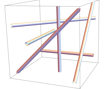
Figure 8: Example of a Mikado flow ${\mathcal{W}}$ restricted to one of the $(\nicefrac{{\mathbb{T}}}{{\lambda}})^{3}$ periodic boxes.

To conclude this section we note that $W_{(\xi)}$ may be written as the $\mathrm{curl\,}$ of a vector field, a fact which is useful in defining the incompressibility corrector in Section 6.5.4. Indeed, since $\xi\cdot\nabla\Phi_{(\xi)}=0$, and since by definition we have that $-\frac{1}{(n_{*}\lambda)^{2}}\Delta\Phi_{(\xi)}=\phi_{(\xi)}$ we obtain

$$\mathrm{curl\,}\left(\frac{1}{(n_{*}\lambda)^{2}}\nabla\Psi_{(\xi)}\times\xi\right)=\mathrm{curl\,}\left(\frac{1}{(n_{*}\lambda)^{2}}\mathrm{curl\,}(\xi\Psi_{(\xi)})\right)=-\xi\left(\frac{1}{(n_{*}\lambda)^{2}}\Delta\Psi_{(\xi)}\right)=W_{(\xi)}\,.$$ (6.31)

For notational simplicity, we define

$$V_{(\xi)}=\frac{1}{(n_{*}\lambda)^{2}}\nabla\Psi_{(\xi)}\times\xi$$ (6.32)

so that $\mathrm{curl\,}V_{(\xi)}=W_{(\xi)}$. With this notation we have the bounds

$$\left\|W_{(\xi)}\right\|_{C^{N}}+\lambda_{q+1}\left\|V_{(\xi)}\right\|_{C^{N}}\lesssim\lambda_{q+1}^{N}$$ (6.33)

for $N\geq 0$.

6.5 The perturbation

In order to define the perturbation $w_{q+1}=v_{q+1}-\overline{v}_{q}$, we need to introduce a few objects.

6.5.1 Cutoffs

Recall that $\mathring{\overline{R}}_{q}$ has support in $\mathbb{T}^{3}\times\cup_{i}I_{i}$, where $I_{i}$ is as defined in (6.9). Accordingly, we define a family of cutoff functions $\{\eta_{i}\}$ with the following properties

1. $\eta_{i}\in C^{\infty}_{x,t}$, $0\leq\eta_{i}\leq 1$, and $\eta_{i}\,\eta_{j}\equiv 0$ for every $i\neq j$ ,

2. $\eta_{i}\equiv 1$, on $\mathbb{T}^{3}\times I_{i}$ ,

3. $\mathrm{supp\,}(\eta_{i})\subset\mathbb{T}^{3}\times\widetilde{I_{i}}$, where $\widetilde{I}_{i}:=J_{i}\cup I_{i}\cup J_{i+1}$,

4. $c_{\eta}\leq\sum_{i}\int_{\mathbb{T}^{3}}\eta_{i}^{2}(x,t)dx\leq 2(2\pi)^{3}$, for all $t\in[0,T]$, where $c_{\eta}>0$ is a universal constant,

5. $\left\|\partial_{t}^{n}\eta_{i}\right\|_{C^{m}}\lesssim_{n,m}\tau_{q}^{-n}$, for all $n,m\geq 0$.

The construction of such a sequence of cutoff functions is elementary (see, e.g. [18, Lemma 5.3]), and Figure 9(a) shows how the supports of the $\eta_{i}$ relate to the support of $\mathring{\overline{R}}_{q}$. We emphasize that condition (iv) is the one which allows us to alter the energy profile of $v_{q+1}$ even on time intervals where $\mathring{\overline{R}}_{q}=0$.

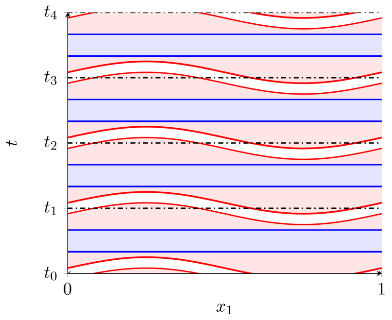
(a) The support of $\mathring{\overline{R}}_{q}$ is given by the blue regions. The support of the cut-off functions $\eta_{i}$, which marks the region where the convex integration perturbation is supported, is given by the region between two consecutive red squiggling stripes.

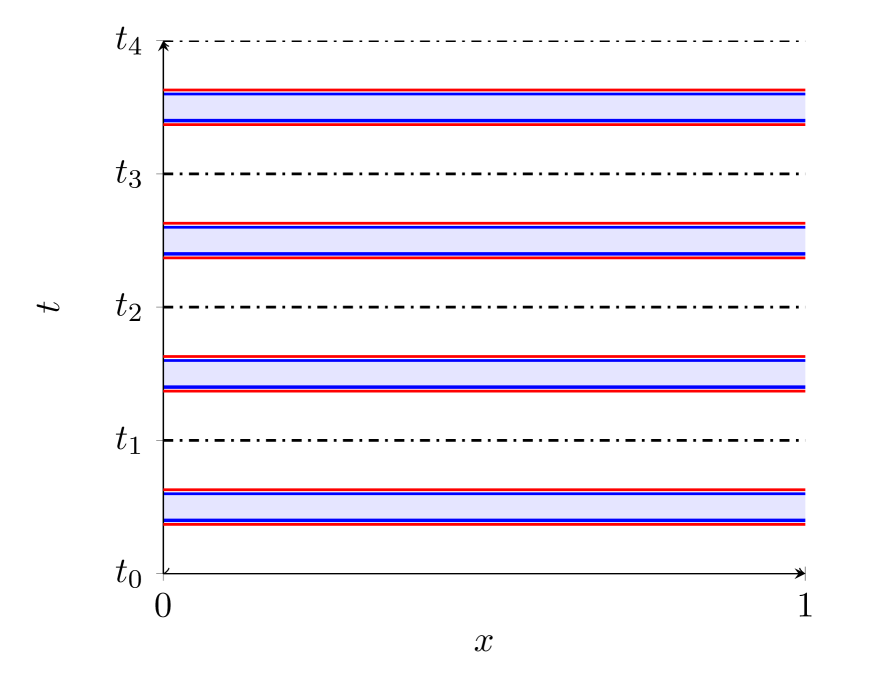
(b) In contrast, in the construction of [102], the support of the convex integration perturbation is (nearly) the same as the support of $\mathring{\overline{R}}_{q}$. Consequently, on the time intervals between two consecutive blue regions, no energy is added to the solution.

Figure 9: The support of $\mathring{\overline{R}}_{q}$ and $w_{q+1}$.

We introduce the function $\rho_{q}(t)$, which measures the remaining energy profile error after the gluing step, and after leaving ourselves room for adding a future velocity increment

$$\rho_{q}(t)=\frac{1}{3}\left(e(t)-\frac{\delta_{q+2}}{2}-\int_{\mathbb{T}^{3}}|\overline{v}_{q}(x,t)|^{2}dx\right)\,.$$

By (6.7d) and (6.20d) we have $\left|\int_{\mathbb{T}^{3}}|v_{q}|^{2}-|\overline{v}_{q}|^{2}\right|\lesssim\delta_{q+1}\ell^{\alpha}$, which may be combined with (6.3d) and the choice of $\ell\leq\lambda_{q}^{-1-\nicefrac{{3\alpha}}{{2}}}$ to deduce that

$$\frac{\delta_{q+1}}{8\lambda_{q}^{\alpha}}\leq\rho_{q}(t)\leq\delta_{q+1}$$ (6.34)

for all $t\in[0,T]$. Similarly, using the assumed bound $\left\|\partial_{t}e\right\|_{C^{0}}\lesssim 1$, the energy inequality for the Euler-Reynolds system obeyed by $(\overline{v}_{q},\mathring{\overline{R}}_{q})$, and the bounds (6.20c) and (6.21a), we obtain

$$\left\|\partial_{t}\rho_{q}\right\|_{C^{0}}\lesssim\delta_{q+1}\delta_{q}^{\nicefrac{{1}}{{2}}}\lambda_{q}\,.$$

The last cutoff function combines $\eta_{i}$ and $\rho_{q}$, and is defined by

$$\rho_{q,i}(x,t)=\rho_{q}(t)\,\frac{\eta_{i}^{2}(x,t)}{\sum_{j}\int_{\mathbb{T}^{3}}\eta_{j}^{2}(y,t)dy}\,.$$ (6.35)

By the normalization of $\rho_{q,i}$ we have that $\sum_{i}\int_{\mathbb{T}^{3}}\rho_{q,i}(x,t)=\rho_{q}(t)$ for all $t\in[0,T]$, and tracing back the properties of $\rho_{q}$ and $\eta_{i}$ we may verify that the following estimates hold

$$\left\|\rho_{q,i}\right\|_{C^{0}}\leq\frac{\delta_{q+1}}{c_{\eta}},\quad\left\|\rho_{q,i}\right\|_{C^{N}}\leq\delta_{q+1},\quad\left\|\partial_{t}\rho_{q,i}\right\|_{C^{N}}\lesssim\delta_{q+1}\tau_{q}^{-1}\,,$$ (6.36)

for all $N\geq 0$, where $c_{\eta}$ is the universal constant from property (iv).

6.5.2 Flow maps

Similarly to Section 5.5.1, we define the (backward) flow maps $\Phi_{i}$ for the velocity field $\overline{v}_{q}$ as the solution of the transport equation

$$(\partial_{t}+\overline{v}_{q}\cdot\nabla)\Phi_{i} =0\,,$$ (6.37a)

$$\Phi_{i}\left(x,t_{i}\right) =x\,,$$ (6.37b)

for all $t\in\mathrm{supp\,}(\eta_{i})\subset\mathbb{T}^{3}\times\widetilde{I}_{i}$. For the reminder of this section, it is convenient to denote the material derivative as $D_{t,q}$, that is

$$D_{t,q}=\partial_{t}+\overline{v}_{q}\cdot\nabla_{x}\,.$$

Since for every $t\in\widetilde{I}_{i}$ we have $|t-t_{i}|\leq 2\tau_{q}$, by the definition of $\tau_{q}$ in (6.8), and using the estimates (6.20c), we have that $\tau_{q}\left\|\nabla\overline{v}_{q}\right\|_{C^{0}}\lesssim\ell^{2\alpha}\ll 1$, and thus the CFL-condition is obeyed on $\widetilde{I}_{i}$. From standard estimates for the transport equation (cf. [16, Proposition D.1]), similarly to the bounds (5.22) discussed earlier, we have

$$\left\|\nabla\Phi_{i}(t)-\mathrm{Id}\right\|_{C^{0}} \lesssim\ell^{2\alpha}\leq\frac{1}{2}$$ (6.38a)

$$\left\|\nabla\Phi_{i}\right\|_{C^{N}}+\left\|(\nabla\Phi_{i})^{-1}\right\|_{C^{N}} \lesssim\ell^{-N}$$ (6.38b)

$$\left\|D_{t,q}\nabla\Phi_{i}\right\|_{C^{N}} \lesssim\delta_{q}^{\nicefrac{{1}}{{2}}}\lambda_{q}\ell^{-N}$$ (6.38c)

for all $t\in\widetilde{I}_{i}$ and $N\geq 0$. In order to establish these bounds it is useful to recall that after applying a gradient to (6.37) we obtain the identity

$$D_{t,q}\nabla\Phi_{i}=-\nabla\Phi_{i}\,D\overline{v}_{q}\,.$$

Also, we note from (6.38a) that $(\nabla\Phi_{i})^{-1}$ is a well-defined object on $\widetilde{I}_{i}$.

6.5.3 Amplitudes

Since $\eta_{i}\equiv 1$ on $\mathbb{T}^{3}\times I_{i}$, $\eta_{i}\eta_{j}\equiv 0$ for $i\neq j$, and since $\mathrm{supp\,}(\mathring{\overline{R}}_{q})\subset\mathbb{T}^{3}\times\cup_{i}I_{i}$, we have that

$$\sum_{i}\eta_{i}^{2}\mathring{\overline{R}}_{q}=\mathring{\overline{R}}_{q}\,.$$ (6.39)

Moreover, the cutoff functions $\eta_{i}$ already incorporate in them a temporal cutoff (recall that $\mathrm{supp\,}(\eta_{i})\subset\mathbb{T}^{3}\times\widetilde{I}_{i}$), and thus it is convenient to introduce

$$R_{q,i}=\rho_{q,i}\mathrm{Id}-\eta_{i}^{2}\,\mathring{\overline{R}}_{q}\,$$

which is a stress supported in $\mathrm{supp\,}(\eta_{i})$, and which obeys $\sum_{i}\mathring{R}_{q,i}=-\mathring{\overline{R}}_{q}$.

For reasons which will become apparent only later (cf. (6.47)), we also define the symmetric tensor

$$\widetilde{R}_{q,i}=\frac{1}{\rho_{q,i}}\nabla\Phi_{i}\,R_{q,i}\,\nabla\Phi_{i}^{T}=\mathrm{Id}+\left(\nabla\Phi_{i}\,\nabla\Phi_{i}^{T}-\mathrm{Id}\right)-\nabla\Phi_{i}\,\frac{\eta_{i}^{2}\mathring{\overline{R}}_{q}}{\rho_{q,i}}\,\nabla\Phi_{i}^{T}$$ (6.40)

for all $(x,t)\in\mathrm{supp\,}(\eta_{i})$. By the above identity, estimate (6.21a) with $N=0$, the property (iv), the bounds (6.34) and (6.38a), we have that

$$\left\|\widetilde{R}_{q,i}(\cdot,t)-\mathrm{Id}\right\|_{C^{0}}\lesssim\ell^{\alpha}\leq\frac{1}{2}\,\qquad\mbox{for all}\qquad t\in\widetilde{I}_{i}\,,$$

once we ensure $a$ is taken to be sufficiently large. Furthermore, using the estimates (6.21), the properties of the $\eta_{i}$, (6.36) and (6.38), one may show that

$$\left\|\widetilde{R}_{q,i}\right\|_{C^{N}}+\tau_{q}\left\|D_{t,q}\widetilde{R}_{q,i}\right\|_{C^{N}}\lesssim\ell^{-N}\,\qquad\mbox{on}\qquad\mathrm{supp\,}(\eta_{i})\,,$$ (6.41)

for all $N\geq 0$. One last important property of the stress $\widetilde{R}_{q,i}$ is the identity

$$\sum_{i}\rho_{q,i}(\nabla\Phi_{i})^{-1}\widetilde{R}_{q,i}(\nabla\Phi_{i})^{-T}=\left(\sum_{i}\rho_{q,i}\right)\mathrm{Id}-\mathring{\overline{R}}_{q}\,,$$ (6.42)

which is useful in cancelling the glued stress. Here we have again appealed to (6.39).

Thus, since $\widetilde{R}_{q,i}$ obeys the conditions of Lemma 6.6 on $\mathrm{supp\,}(\eta_{i})$, and since $\rho_{q,i}^{\nicefrac{{1}}{{2}}}$ is a multiple of $\eta_{i}$, we may define the amplitude functions

$$a_{(\xi,i)}(x,t)=\rho_{q,i}(x,t)^{\nicefrac{{1}}{{2}}}\,\gamma_{\xi}(\widetilde{R}_{q,i})$$ (6.43)

where the $\gamma_{\xi}$ are the functions from Lemma 6.6. Note importantly that the amplitude functions already include a temporal cutoff, which shows that $\mathrm{supp\,}(a_{(\xi,i)})\subset\mathrm{supp\,}(\eta_{i})$. The amplitude functions $a_{(\xi)}$ inherit the expected $C^{N}$ bounds and material derivative bounds from (6.36), (6.41), the product at the chain rules

$$\left\|a_{(\xi,i)}\right\|_{C^{N}}+\tau_{q}\left\|D_{t,q}a_{(\xi,i)}\right\|_{C^{N}}\lesssim\delta_{q+1}^{\nicefrac{{1}}{{2}}}\ell^{-N}$$ (6.44)

for $N\geq 0$.

6.5.4 Principal part of the velocity increment and the incompressibility corrector

For the remainder of the paper we consider Mikado building blocks as defined in (6.26) with $\lambda=\lambda_{q+1}$, i.e.

$$W_{(\xi)}(x)=W_{\xi,\lambda_{q+1}}(x)\,.$$

Recall: for the index sets $\Lambda_{i}$ of Lemma 6.6, we overload notation and write $\Lambda_{i}=\Lambda_{0}$ for $i$ even, and $\Lambda_{i}=\Lambda_{1}$ for $i$ odd. With this notation, we now define the principal part of the velocity increment as

$$w_{q+1}^{(p)}(x,t)=\sum_{i}\sum_{\xi\in\Lambda_{i}}a_{(\xi,i)}(x,t)(\nabla\Phi_{i}(x,t))^{-1}W_{(\xi)}(\Phi_{i}(x,t))\,.$$ (6.45)

When compared to the ansatz we made earlier for the $C^{0+}$ result (see (5.27)–(5.28)), we notice the presence of $(\nabla\Phi_{i})^{-1}$. The reason for this modification is as follows. At time $t=t_{i}$, we have $\Phi_{i}(x,t_{i})=x$, $\nabla\Phi_{i}=\mathrm{Id}$, and by (6.27) we have that the vector field

$$U_{i,\xi}=(\nabla\Phi_{i})^{-1}W_{(\xi)}(\Phi_{i})$$

is incompressible at $t=t_{i}$. We then notice that $U_{i,\xi}$ is Lie-advected by the flow of the incompressible vector field $\overline{v}_{q}$, in the sense that

$$D_{t,q}U_{i,\xi}=(U_{i,\xi}\cdot\nabla)\overline{v}_{q}=(\nabla\overline{v}_{q})^{T}U_{i,\xi}\,.$$ (6.46)

This implies directly that $D_{t,q}(\mathrm{div\,}U_{i,\xi})=0$, and thus the divergence free nature of $U_{i,\xi}$ is carried from $t=t_{i}$ to all $t$ close to $t_{i}$. This shows that the function $w_{q+1}^{(p)}$ defined in (6.45) is to leading order in $\lambda_{q+1}$ divergence-free (i.e. the incompressibility corrector will turn out to be small).

At this stage we may also explain why $R_{q,i}$ was not just normalized by $\rho_{q,i}$ but also conjugated with $\nabla\Phi_{i}$ respectively $(\nabla\Phi_{i})^{T}$, in order to obtain $\widetilde{R}_{q,i}$ (cf. (6.40)). Using the spanning property of the Mikado building blocks (6.30), the fact that they have mutually disjoint support (6.28), identity (6.42) above, and the fact that the $\eta_{i}$ have mutually disjoint supports, we obtain

$$w_{q+1}^{(p)}\otimes w_{q+1}^{(p)}=\sum_{i}\sum_{\xi\in\Lambda_{i}}a_{(\xi,i)}^{2}(\nabla\Phi_{i})^{-1}\left((W_{(\xi)}\circ\Phi_{i})\otimes(W_{(\xi)}\circ\Phi_{i})\right)(\nabla\Phi_{i})^{-T}$$

$$=\sum_{i}\rho_{q,i}(\nabla\Phi_{i})^{-1}\left(\sum_{\xi\in\Lambda_{i}}\gamma_{\xi}^{2}(\widetilde{R}_{q,i})\left((W_{(\xi)}\otimes W_{(\xi)})\circ\Phi_{i}\right)\right)(\nabla\Phi_{i})^{-T}$$

$$=\sum_{i}\rho_{q,i}(\nabla\Phi_{i})^{-1}\widetilde{R}_{q,i}(\nabla\Phi_{i})^{-T}+\sum_{i}\sum_{\xi\in\Lambda_{i}}a_{(\xi,i)}^{2}(\nabla\Phi_{i})^{-1}\left(\left(\mathbb{P}_{\neq 0}(W_{(\xi)}\otimes W_{(\xi)})\right)\circ\Phi_{i}\right)(\nabla\Phi_{i})^{-T}$$

$$=\left(\sum_{i}\rho_{q,i}\right)\mathrm{Id}-\mathring{\overline{R}}_{q}+\sum_{i}\sum_{\xi\in\Lambda_{i}}a_{(\xi,i)}^{2}(\nabla\Phi_{i})^{-1}\left(\left(\mathbb{P}_{\geq\nicefrac{{\lambda_{q+1}}}{{2}}}(W_{(\xi)}\otimes W_{(\xi)})\right)\circ\Phi_{i}\right)(\nabla\Phi_{i})^{-T}$$ (6.47)

where we have denoted by $\mathbb{P}_{\neq 0}f(x)=f(x)-\fint_{\mathbb{T}^{3}}f(y)dy$, the projection of $f$ onto its nonzero frequencies. We have also used that since $W_{(\xi)}\otimes W_{(\xi)}$ is $(\nicefrac{{\mathbb{T}}}{{\lambda_{q+1}}})^{3}$-periodic, the identity $\mathbb{P}_{\neq 0}(W_{(\xi)}\otimes W_{(\xi)})=\mathbb{P}_{\geq\nicefrac{{\lambda_{q+1}}}{{2}}}(W_{(\xi)}\otimes W_{(\xi)})$ holds. The calculation (6.47) shows that by design, the low frequency part of $w_{q+1}^{(p)}\otimes w_{q+1}^{(p)}$ cancels the glued stress $\mathring{\overline{R}}_{q}$, modulo a multiple of the identity, which is then used to correct the energy profile and which contributes a pressure term to the equation.

Based on the definition (6.45) of the principal part of the velocity increment, we construct an incompressibility corrector. As was observed in [44], for any smooth vector field $V$, we have the identity

$$(\nabla\Phi_{i})^{-1}\left((\mathrm{curl\,}V)\circ\Phi_{i}\right)=\mathrm{curl\,}\left((\nabla\Phi_{i})^{T}(V\circ\Phi_{i})\right).$$

Recalling identity (6.31) and the definition (6.32), we may write $W_{(\xi)}=\mathrm{curl\,}V_{(\xi)}$ and thus the above identity shows that

$$(\nabla\Phi_{i})^{-1}(W_{(\xi)}\circ\Phi_{i})=\mathrm{curl\,}\left((\nabla\Phi_{i})^{T}(V_{(\xi)}\circ\Phi_{i})\right)\,.$$

From the above identity and (6.45), it follows that if we define the incompressibility corrector as

$$w_{q+1}^{(c)}(x,t)=\sum_{i}\sum_{\xi\in\Lambda_{i}}\nabla a_{(\xi,i)}(x,t)\times\left((\nabla\Phi_{i}(x,t))^{T}(V_{(\xi)}(\Phi_{i}(x,t))\right)$$ (6.48)

then the total velocity increment $w_{q+1}$ obeys

$$w_{q+1}=w_{q+1}^{(p)}+w_{q+1}^{(c)}=\mathrm{curl\,}\left(\sum_{i}\sum_{\xi\in\Lambda_{i}}a_{(\xi,i)}\,(\nabla\Phi_{i})^{T}(V_{(\xi)}\circ\Phi_{i})\right)$$ (6.49)

so that it is automatically incompressible.

6.5.5 Velocity inductive estimates

The velocity field at level $q+1$ is constructed as

$$v_{q+1}=\overline{v}_{q}+w_{q+1}=v_{q}+(v_{\ell}-v_{q})+(\overline{v}_{q}-v_{\ell})+w_{q+1}\,.$$ (6.50)

From (6.22), (6.36), (6.38a), (6.43), and (6.45), and the fact that the $\eta_{i}$ have disjoint supports, once $a$ is sufficiently large we obtain that

$$\left\|w_{q+1}^{(p)}\right\|_{C^{0}} \leq\frac{2|\Lambda_{i}|\left\|\phi\right\|_{C^{0}}}{c_{\eta}^{\nicefrac{{1}}{{2}}}C_{\Lambda}}M\delta_{q+1}^{\nicefrac{{1}}{{2}}}\leq\frac{M}{8}\delta_{q+1}^{\nicefrac{{1}}{{2}}}$$ (6.51a)

$$\left\|w_{q+1}^{(p)}\right\|_{C^{1}} \leq\frac{4|\Lambda_{i}|n_{*}\left\|\phi\right\|_{C^{1}}}{c_{\eta}^{\nicefrac{{1}}{{2}}}C_{\Lambda}}M\delta_{q+1}^{\nicefrac{{1}}{{2}}}\lambda_{q+1}\leq\frac{M}{8}\delta_{q+1}^{\nicefrac{{1}}{{2}}}\lambda_{q+1}$$ (6.51b)

by choosing the parameter $C_{\Lambda}$ from (6.22) to be large enough. Note that $C_{\Lambda}$ only depends on the cardinality of $\Lambda_{i}$, on the universal constant $c_{\eta}$, the geometric integer $n_{*}$, and on the $C^{1}$ norm of the function $\phi$, which in turn depends solely on the geometric constant $\varepsilon_{\Lambda}$.

For the incompressibility corrector we lose a factor of $\ell^{-1}$ from the gradient landing on $a_{(\xi,i)}$, but we gain a factor of $\lambda_{q+1}$ because we have $V_{(\xi)}$ instead of $W_{(\xi)}$ (recall (6.32)). Therefore, we may show that

$$\left\|w_{q+1}^{(c)}\right\|_{C^{0}}+\frac{1}{\lambda_{q+1}}\left\|w_{q+1}^{(c)}\right\|_{C^{1}}\lesssim\delta_{q+1}^{\nicefrac{{1}}{{2}}}\frac{\ell^{-1}}{\lambda_{q+1}}\,.$$ (6.52)

We note that by choosing $\alpha$ to be sufficiently small in therms of $b$ and $\beta$, we have

$$\frac{\ell^{-1}}{\lambda_{q+1}}=\frac{\delta_{q}^{\nicefrac{{1}}{{2}}}\lambda_{q}^{1+\nicefrac{{3\alpha}}{{2}}}}{\delta_{q+1}^{\nicefrac{{1}}{{2}}}\lambda_{q+1}}=\frac{\lambda_{q}^{1-\beta+\nicefrac{{3\alpha}}{{2}}}}{\lambda_{q+1}^{1-\beta}}\leq 2\lambda_{q}^{\nicefrac{{3\alpha}}{{2}}-(b-1)(1-\beta)}\leq\lambda_{q}^{-\nicefrac{{(b-1)(1-\beta)}}{{2}}}\ll 1\,,$$ (6.53)

and thus by choosing $a$ sufficiently large we may ensure that the velocity increment defined in (6.48) obeys

$$\left\|w_{q+1}\right\|_{C^{0}}+\frac{1}{\lambda_{q+1}}\left\|w_{q+1}\right\|_{C^{1}}\leq\frac{M}{2}\delta_{q+1}^{\nicefrac{{1}}{{2}}}\,.$$

By combining the above estimate with (6.7), (6.20), and (6.50), after choosing $a$ sufficiently large, we deduce that (6.4) is satisfied, and moreover that the bounds (6.3b) and (6.3c) hold with $q$ replaced with $q+1$.

6.6 Reynolds stress

Recall that the pair $(\overline{v}_{q},\mathring{\overline{R}}_{q})$ solves the Euler-Reynolds system (4.2), and that $v_{q+1}$ is defined in (6.50). In this subsection we define the new Reynolds stress $\mathring{R}_{q+1}$, and show that it obeys the estimate

$$\left\|\mathring{R}_{q+1}\right\|_{C^{\alpha}}\lesssim\frac{\delta_{q+1}^{\nicefrac{{1}}{{2}}}\delta_{q}^{\nicefrac{{1}}{{2}}}\lambda_{q}}{\lambda_{q+1}^{1-4\alpha}}\,.$$ (6.54)

The above bound immediately implies the desired estimate (6.3a) at level $q+1$, upon noting that the following parameter inequality holds (after taking $\alpha$ sufficiently small and $a$ sufficiently large)

$$\frac{\delta_{q+1}^{\nicefrac{{1}}{{2}}}\delta_{q}^{\nicefrac{{1}}{{2}}}\lambda_{q}}{\lambda_{q+1}^{1-4\alpha}}\leq\frac{\delta_{q+2}}{\lambda_{q+1}^{4\alpha}}\,.$$ (6.55)

The remaining power of $\lambda_{q+1}^{-\alpha}$ is used to absorb the implicit constant in (6.54).

In order to define $\mathring{R}_{q+1}$, similarly to (5.41) we write

$$\mathrm{div\,}\mathring{R}_{q+1}-\nabla p_{q+1} =\underbrace{D_{t,q}w^{(p)}_{q+1}}_{\mathrm{div\,}(R_{\rm transport})}+\underbrace{\mathrm{div\,}(w_{q+1}^{(p)}\otimes w_{q+1}^{(p)}+\mathring{\overline{R}}_{q})}_{\mathrm{div\,}(R_{\rm oscillation})+\nabla p_{\rm oscillation}}+\underbrace{w_{q+1}\cdot\nabla\overline{v}_{q}}_{\mathrm{div\,}(R_{\rm Nash})}$$

$$\qquad+\underbrace{D_{t,q}w^{(c)}_{q+1}+\mathrm{div\,}\left(w_{q+1}^{(c)}\otimes w_{q+1}+w_{q+1}^{(p)}\otimes w_{q+1}^{(c)}\right)}_{\mathrm{div\,}(R_{\rm corrector})+\nabla p_{\rm corrector}}-\nabla\overline{p}_{q}\,.$$ (6.56)

The various traceless symmetric stresses present implicitly in (6.56) are defined using the inverse divergence operator $\mathcal{R}$, and by recalling the identity (6.47) (for the oscillation error) as

$$R_{\rm transport} =\mathcal{R}\left(D_{t,q}w^{(p)}_{q+1}\right)$$ (6.57a)

$$R_{\rm oscillation} =\sum_{i}\sum_{\xi\in\Lambda_{i}}\mathcal{R}\mathrm{div\,}\left(a_{(\xi,i)}^{2}(\nabla\Phi_{i})^{-1}\left(\left(\mathbb{P}_{\geq\nicefrac{{\lambda_{q+1}}}{{2}}}(W_{(\xi)}\otimes W_{(\xi)})\right)\circ\Phi_{i}\right)(\nabla\Phi_{i})^{-T}\right)$$ (6.57b)

$$R_{\rm Nash} =\mathcal{R}\left(w_{q+1}\cdot\nabla\overline{v}_{q}\right)$$ (6.57c)

$$R_{\rm corrector} =\mathcal{R}\left(D_{t,q}w^{(c)}_{q+1}\right)+\left(w_{q+1}^{(c)}\mathring{\otimes}w_{q+1}^{(c)}+w_{q+1}^{(c)}\mathring{\otimes}w_{q+1}^{(p)}+w_{q+1}^{(p)}\mathring{\otimes}w_{q+1}^{(c)}\right)$$ (6.57d)

while the pressure terms are given by $p_{\rm oscillation}=\sum_{i}\rho_{q,i}$ and $p_{\rm corrector}=2w_{q+1}^{(c)}\cdot w_{q+1}^{(p)}+|w_{q+1}^{(c)}|^{2}$. With this notation we have $p_{q+1}=\overline{p}_{q}-p_{\rm oscillation}-p_{\rm corrector}$ and

$$\mathring{R}_{q+1}=R_{\rm transport}+R_{\rm oscillation}+R_{\rm Nash}+R_{\rm corrector}\,.$$ (6.58)

Prior to estimating the above stresses, it is convenient to adapt the stationary phase bounds of Section 5.6.1 from Beltrami flows to Mikado flows.

6.6.1 Inverse divergence and stationary phase bounds

In order to apply Lemma 5.7, and obtain bounds similar to (5.39) and (5.40), but for Mikado flows instead of the Beltrami flows, we decompose the function $\phi_{(\xi)}$ which defined $W_{(\xi)}$ in (6.26) as a Fourier series. Recall that $\phi_{(\xi)}$ defined in (6.25) is $(\nicefrac{{\mathbb{T}}}{{\lambda_{q+1}}})^{3}$ periodic and has zero mean. Additionally, the function $\phi$ is $C^{\infty}$ smooth. Therefore, we may decompose

$$\phi_{(\xi)}(x)=\phi_{\xi,\lambda_{q+1}}(x)=\sum_{k\in\mathbb{Z}^{3}\setminus\{0\}}f_{\xi}(k)e^{i\lambda_{q+1}k\cdot(x-\alpha_{\xi})}\,$$ (6.59)

where the complex numbers $f_{\xi}(k)$ are the Fourier series coefficients of the $C^{\infty}$ smooth, mean-zero $\mathbb{T}^{3}$ periodic function $z\mapsto\phi(n_{*}z\cdot A_{\xi},n_{*}z\cdot(\xi\times A_{\xi}))$. The shift $x\mapsto x-\alpha_{\xi}$ has no effect on the estimates. Moreover, the Fourier coefficients decay arbitrarily fast. For any $m\in\mathbb{N}$ we have $|f_{\xi}(k)|=|f_{\xi}(k)e^{i\lambda_{q+1}k\cdot\alpha_{\xi}}|\leq C|k|^{-m}$, where the constant $C$ depends on $m$ and on geometric parameters of the construction, such as $n_{*}$, the sets $\Lambda_{i}$, the shifts $\alpha_{\xi}$, and norms of the bump function $\phi(x_{1},x_{2})$. Thus, $C$ is independent of $\lambda_{q+1}$, or any other $q$-dependent parameter.

A similar Fourier series decomposition applies to the function $\frac{1}{n_{*}\lambda_{q+1}}\nabla\Psi_{(\xi)}=(\nabla\Psi)_{(\xi)}$ which is used in (6.32) to define $V_{(\xi)}$. For this function we also obtain that its Fourier series coefficients decay arbitrarily fast, with constants that are bounded independently of $q$ (and hence $\lambda_{q+1}$).

Therefore, for a smooth function $a(x,t)$, in order to estimate $\mathcal{R}(a\,W_{(\xi)}\circ\Phi_{i})$, we use identity (6.59), and apply Lemma 5.7 for each $k$ individually, and then sum in $k$ using the fast decay of the Fourier coefficients $f_{\xi}(k)$. Without giving all the details, we summarize this procedure as follows. Let $a\in C^{0}([0,T];C^{m,\alpha}(\mathbb{T}^{3}))$ be such that $\mathrm{supp\,}(a)\subset\mathrm{supp\,}(\eta_{i})$, which ensures that the phase $\Phi_{i}$ obeys the conditions of Lemma 5.7 by (6.38a). Using (6.38b) we obtain from Lemma 5.7 that

$$\left\|\mathcal{R}\left(a\;(W_{(\xi)}\circ\Phi_{i})\right)\right\|_{C^{\alpha}}+\lambda_{q+1}\left\|\mathcal{R}\left(a\;(V_{(\xi)}\circ\Phi_{i})\right)\right\|_{C^{\alpha}}\lesssim\frac{\left\|a\right\|_{C^{0}}}{\lambda_{q+1}^{1-\alpha}}+\frac{\left\|a\right\|_{C^{m,\alpha}}+\left\|a\right\|_{C^{0}}\ell^{-m-\alpha}}{\lambda_{q+1}^{m-\alpha}}\,,$$ (6.60)

where the implicit constant is independent of $q$.

Recalling that $W_{(\xi)}\otimes W_{(\xi)}=(\xi\otimes\xi)\phi_{(\xi)}^{2}$, and using that the function $\mathbb{P}_{\geq\nicefrac{{\lambda_{q+1}}}{{2}}}\phi_{(\xi)}^{2}$ is also zero mean $(\nicefrac{{\mathbb{T}}}{{\lambda_{q+1}}})^{3}$-periodic, a similar argument shows that

$$\left\|\mathcal{R}\left(a\;\left(\Big{(}\mathbb{P}_{\geq\nicefrac{{\lambda_{q+1}}}{{2}}}(W_{(\xi)}\otimes W_{(\xi)})\Big{)}\circ\Phi_{i}\right)\right)\right\|_{C^{\alpha}}\lesssim\frac{\left\|a\right\|_{C^{0}}}{\lambda_{q+1}^{1-\alpha}}+\frac{\left\|a\right\|_{C^{m,\alpha}}+\left\|a\right\|_{C^{0}}\ell^{-m-\alpha}}{\lambda_{q+1}^{m-\alpha}}$$ (6.61)

holds. The above estimate is useful for estimating the oscillation error.

6.6.2 The estimate for $\mathring{R}_{q+1}$

In this section we show that the stresses defined in (6.58) obey (6.54). The Nash error and the corrector error are in a sense lower order, and they can be treated similarly (or using similar bounds) to the transport and oscillation errors. Because of this, we omit the details for estimating $R_{\rm Nash}$ and $R_{\rm corrector}$.

Transport error.   Recalling the definition of $w_{q+1}^{(p)}$ in (6.45), and the Lie-advection identity (6.46) we obtain that the transport stress in (6.57a) is given by

$$R_{\rm transport} =\sum_{i}\sum_{\xi\in\Lambda_{i}}\mathcal{R}\left(a_{(\xi,i)}(\nabla\overline{v}_{q})^{T}(\nabla\Phi_{i})^{-1}W_{(\xi)}(\Phi_{i})\right)+\mathcal{R}\left(\left(D_{t,q}a_{(\xi,i)}\right)(\nabla\Phi_{i})^{-1}W_{(\xi)}(\Phi_{i})\right)\,.$$ (6.62)

In order to bound the terms in (6.62) we use (6.60) to gain a factor of $\lambda_{q+1}^{-1+\alpha}$ from the operator $\mathcal{R}$ acting on the highest frequency term $W_{(\xi)}\circ\Phi_{i}$. The derivatives of $a_{(\xi,i)}$, $\nabla\overline{v}_{q}$, and $(\nabla\Phi_{i})^{-1}$ are estimated using (6.44), (6.20c), and (6.38b) respectively. These bounds show that each additional spacial derivatives costs a power of $\ell^{-1}$. We obtain from (6.60) that

$$\left\|R_{\rm transport}\right\|_{C^{\alpha}} \lesssim\frac{\delta_{q+1}^{\nicefrac{{1}}{{2}}}\delta_{q}^{\nicefrac{{1}}{{2}}}\lambda_{q}}{\lambda_{q+1}^{1-\alpha}}\left(1+\frac{\ell^{-m-\alpha}}{\lambda_{q+1}^{m-1}}\right)+\frac{\delta_{q+1}^{\nicefrac{{1}}{{2}}}\tau_{q}^{-1}}{\lambda_{q+1}^{1-\alpha}}\left(1+\frac{\ell^{-m-\alpha}}{\lambda_{q+1}^{m-1}}\right)\,.$$

Recalling (6.53), we have that $(\ell\lambda_{q+1})^{-1}\leq\lambda_{q}^{-\nicefrac{{(b-1)(1-\beta)}}{{2}}}$, and thus upon taking the parameter $m$ in to be sufficiently large (in terms of $\beta$ and $b$), we obtain that $R_{\rm transport}$ indeed is bounded by the right side of (6.54), as desired.

Oscillation error.   For the oscillation error, which is defined in (6.57b), the main observation is that when the $\mathrm{div\,}$ operator lands on the highest frequency term, namely $\left(\mathbb{P}_{\geq\nicefrac{{\lambda_{q+1}}}{{2}}}(W_{(\xi)}\otimes W_{(\xi)})\right)\circ\Phi_{i}$, due to certain cancellations this term vanishes. Since by construction we have $(\xi\cdot\nabla)\phi_{(\xi)}=0$ it also follows that $(\xi\cdot\nabla)\mathbb{P}_{\geq\nicefrac{{\lambda_{q+1}}}{{2}}}(\phi_{(\xi)}^{2})=0$. Therefore,

$$\mathrm{div\,}\left(a_{(\xi,i)}^{2}(\nabla\Phi_{i})^{-1}\left(\left(\mathbb{P}_{\geq\nicefrac{{\lambda_{q+1}}}{{2}}}(W_{(\xi)}\otimes W_{(\xi)})\right)\circ\Phi_{i}\right)(\nabla\Phi_{i})^{-T}\right)$$

$$=\mathrm{div\,}\left(a_{(\xi,i)}^{2}(\nabla\Phi_{i})^{-1}(\xi\otimes\xi)(\nabla\Phi_{i})^{-T}\left(\left(\mathbb{P}_{\geq\nicefrac{{\lambda_{q+1}}}{{2}}}(\phi_{(\xi)}^{2})\right)\circ\Phi_{i}\right)\right)$$

$$=\left(\left(\mathbb{P}_{\geq\nicefrac{{\lambda_{q+1}}}{{2}}}(\phi_{(\xi)}^{2})\right)\circ\Phi_{i}\right)\mathrm{div\,}\left(a_{(\xi,i)}^{2}(\nabla\Phi_{i})^{-1}(\xi\otimes\xi)(\nabla\Phi_{i})^{-T}\right)$$

$$\qquad+\underbrace{a_{(\xi,i)}^{2}(\nabla\Phi_{i})^{-1}(\xi\otimes\xi)(\nabla\Phi_{i})^{-T}\left((\nabla\Phi_{i})^{T}\left(\nabla\mathbb{P}_{\geq\nicefrac{{\lambda_{q+1}}}{{2}}}(\phi_{(\xi)}^{2})\right)\circ\Phi_{i}\right)}_{=0}.$$

The above identity shows that

$$R_{\rm oscillation}=\sum_{i}\sum_{\xi\in\Lambda_{i}}\mathcal{R}\left(\left(\left(\mathbb{P}_{\geq\nicefrac{{\lambda_{q+1}}}{{2}}}(W_{(\xi)}\otimes W_{(\xi)})\right)\circ\Phi_{i}\right)\mathrm{div\,}\left(a_{(\xi,i)}^{2}(\nabla\Phi_{i})^{-1}(\xi\otimes\xi)(\nabla\Phi_{i})^{-T}\right)\right)\,,$$

at which point we may appeal to the stationary phase estimate (6.61) combined with the bounds (6.44) and (6.38b) to obtain

$$\left\|R_{\rm oscillation}\right\|_{C^{\alpha}}\lesssim\frac{\delta_{q+1}\ell^{-1}}{\lambda_{q+1}^{1-\alpha}}\left(1+\frac{\ell^{-m-\alpha}}{\lambda_{q+1}^{m-1}}\right)\lesssim\frac{\delta_{q+1}^{\nicefrac{{1}}{{2}}}\delta_{q}^{\nicefrac{{1}}{{2}}}\lambda_{q}}{\lambda_{q+1}^{1-\nicefrac{{5\alpha}}{{2}}}}\,.$$

Here we have again taken $m$ sufficiently large, and have recalled the definition of $\ell$ in (6.6). Thus the oscillation error is also bounded by the right side of (6.54), as claimed.

6.6.3 Energy increment

To conclude the proof of Proposition 6.3, it remains to show that (6.3d) holds with $q$ replaced by $q+1$. In order to prove this bound we show that

$$\left|e(t)-\int_{\mathbb{T}^{3}}|v_{q+1}(x,t)|^{2}dx-\frac{\delta_{q+2}}{2}\right|\lesssim\frac{\delta_{q+1}^{\nicefrac{{1}}{{2}}}\delta_{q}^{\nicefrac{{1}}{{2}}}\lambda_{q}^{1+2\alpha}}{\lambda_{q+1}}$$ (6.63)

holds. Recalling the parameter estimate (6.55), and taking $a$ sufficiently large to absorb all the implicit constants, it is clear that (6.63) implies the bound (6.3d) at level $q+1$.

In order to prove (6.63), the principal observation is the following. Taking the trace of (6.47), since $\mathring{\overline{R}}_{q}$ is traceless we obtain

$$\int_{\mathbb{T}^{3}}|w_{q+1}|^{2}dx =3\sum_{i}\int_{\mathbb{T}^{3}}{\rho_{q,i}}dx$$

$$+\sum_{i}\sum_{\xi\in\Lambda_{i}}\int_{\mathbb{T}^{3}}a_{(\xi,i)}^{2}\mathrm{tr\,}\left((\nabla\Phi_{i})^{-1}(\xi\otimes\xi)(\nabla\Phi_{i})^{-T}\right)\left(\left(\mathbb{P}_{\geq\nicefrac{{\lambda_{q+1}}}{{2}}}(W_{(\xi)}\otimes W_{(\xi)})\right)\circ\Phi_{i}\right)dx\,.$$

The second term in the above identity can be made arbitrarily small, since it is the $L^{2}$ inner product of a function whose oscillation frequency is $\lesssim\ell^{-1}$ (cf. (6.44) and (6.38b)) and a function which is $\lambda_{q+1}$ periodic and zero mean. On the other hand, by the design of the functions $\rho_{q,i}$ (cf. (6.35)) we have

$$3\sum_{i}\int_{\mathbb{T}^{3}}{\rho_{q,i}}dx=3\rho_{q}(t)=e(t)-\frac{\delta_{q+2}}{2}-\int_{\mathbb{T}^{3}}|\overline{v}_{q}(x,t)|^{2}dx\,.$$

Since $v_{q+1}=\overline{v}_{q}+w_{q+1}$, the above identity implies that

$$e(t)-\int_{\mathbb{T}^{3}}|v_{q+1}(x,t)|^{2}dx-\frac{\delta_{q+2}}{2}=-2\int_{\mathbb{T}^{3}}\overline{v}_{q}\cdot w_{q+1}dx-2\int_{\mathbb{T}^{3}}w_{q+1}^{(p)}\cdot w_{q+1}^{(c)}dx-\int_{\mathbb{T}^{3}}|w_{q+1}^{(c)}|dx\,.$$

The corrector terms in the above give estimates consistent with (6.63) by appealing to (6.51a), (6.52), and (6.53). For the first term on the right side of the above we recall (cf. (6.49)) that $w_{q+1}$ may be written as the $\mathrm{curl\,}$ of a vector field whose size is $\delta_{q+1}^{\nicefrac{{1}}{{2}}}\lambda_{q+1}^{-1}$. Integrating by parts the $\mathrm{curl\,}$ and using (6.20c) with $N=0$ we conclude the proof of (6.63), and hence of Proposition 6.3.

7 Navier-Stokes: existence of weak solutions with finite energy

We consider weak solutions of the Navier-Stokes equations (1.1) (see Definition 3.6 above). The viscosity parameter obeys $\nu\in(0,1]$, and we consider solutions $v$ which have zero mean on $\mathbb{T}^{3}$. The main result of [20] is Theorem 3.7.

In order to keep the exposition as simple as possible, without omitting any of the main ideas involved in proving Theorem 3.7, in this section we prove a simpler result which states that there exists a weak solution in the aforementioned regularity class, whose kinetic energy is not monotone decreasing. Thus, this weak solution is not equal to any of the Leray-Hopf weak solutions arising from the same $L^{2}$ initial datum $v|_{t=0}$.

Theorem 7.1.

There exists $\beta>0$, such that the following holds. There exists a sufficiently small $\nu\in(0,1]$ and a weak solution $v$ of the Navier-Stokes equations (1.1), which lies in $C^{0}([0,1];H^{\beta}(\mathbb{T}^{3}))\cap C^{0}([0,1];W^{1,1+\beta}(\mathbb{T}^{3}))$, and such that $\left\|v(\cdot,1)\right\|_{L^{2}}\geq 2\left\|v(\cdot,0)\right\|_{L^{2}}$.

Theorem 7.1 is proven in Section 7.2 below. This proof can be used to also establish Theorem 3.7 if one adds a few inductive estimates to the the list in (7.2) below, cf. (2.4)–(2.6) in [20]. For simplicity we omit these details here, and only prove this more restrictive result.

7.1 Inductive estimates

Let $(v_{q},\mathring{R}_{q})$ be a given solution of the Navier-Stokes-Reynolds system (4.7). We consider the same parameters $\lambda_{q}\to+\infty$ and $\delta_{q}\to 0^{+}$ defined by

$$\lambda_{q} =2\pi a^{(b^{q})}$$ (7.1a)

$$\delta_{q} =\lambda_{q}^{-2\beta}\,.$$ (7.1b)

The sufficiently large (universal) parameter $b$ is free, and so is the sufficiently small parameter $\beta=\beta(b)$. The parameter $a$ is chosen to be a sufficiently large multiple of the geometric constant $n_{*}$ from (6.23) above.

For $q\geq 0$ we make the following inductive assumptions

$$\left\|v_{q}\right\|_{L^{2}} \leq 1-\delta_{q}^{\nicefrac{{1}}{{2}}}$$ (7.2a)

$$\left\|v_{q}\right\|_{C^{1}_{x,t}} \leq\lambda_{q}^{4}$$ (7.2b)

$$\left\|\mathring{R}_{q}\right\|_{L^{1}} \leq c_{R}\delta_{q+1}$$ (7.2c)

where $c_{R}>0$ is a sufficiently small universal constant (determined in (7.34) in terms of the parameter $M$ from Lemma 6.6 below). The inductive proposition is almost identical to Proposition 5.3.

Proposition 7.2 (Main iteration).

There exists a sufficiently large universal parameter $b>1$, and a sufficiently small parameter $\beta=\beta(b)>0$, such that the following holds. There exists a sufficiently large constant $a_{0}=a_{0}(c_{R},\beta,b)$ such that for any $a\geq a_{0}$ which is a multiple of the geometric constant $n_{*}$, there exist functions $(v_{q+1},\mathring{R}_{q+1})$ which solve (4.7) and obey (7.2) at level $q+1$, such that

$$\left\|v_{q+1}-v_{q}\right\|_{L^{2}}\leq\delta_{q+1}^{\nicefrac{{1}}{{2}}}$$ (7.3)

holds. All parameters in the Proposition, $b$, $\beta$, and $a_{0}$, are independent of $\nu\in(0,1]$ .

Remark 7.3 (Quantifying the parameters $\beta$ and $b$).

For the purpose of specifying the parameters $b$ and $\beta$ it is convenient to first fix an auxiliary parameter $0<\alpha\ll 1$. It is sufficient to take $\alpha\leq\nicefrac{{1}}{{240}}$, arbitrary. Then, inspecting the proof of Proposition 7.2, we may verify that $b\in\mathbb{N}$ may be chosen to be any multiple of $7$ which obeys $b>\nicefrac{{4}}{{\alpha}}$. With such a value of $b$ fixed, $\beta$ may be chosen to obey $\beta<\nicefrac{{\alpha}}{{b}}$. We did not try here to optimize these conditions. The particular choices $\alpha=\nicefrac{{1}}{{240}}$, $b=1001$, and $\beta=\nicefrac{{1}}{{2^{18}}}$ are permissible.

7.2 Proof of Theorem 7.1

Fix the parameters $b,\beta,c_{R}$ and $a_{0}$ from Proposition 7.2. By possibly enlarging the value of $a\geq a_{0}$, we may ensure that $\delta_{0}\leq\nicefrac{{1}}{{4}}$.

We define an incompressible, zero mean vector field $v_{0}$ by

$$v_{0}(x,t)=\frac{t}{(2\pi)^{\nicefrac{{3}}{{2}}}}(\sin(\lambda_{0}x_{3}),0,0)$$

and define the kinematic viscosity

$$\nu=\lambda_{0}^{-2}\in(0,1]\,.$$

Note that by construction we have $\sup_{t\in[0,1]}\left\|v_{0}(\cdot,t)\right\|_{L^{2}}\leq\left\|v_{0}(\cdot,1)\right\|_{L^{2}}=\nicefrac{{1}}{{\sqrt{2}}}\leq 1-\delta_{0}^{\nicefrac{{1}}{{2}}}$, so that (7.2a) is automatically satisfied. Moreover, $\left\|v_{0}\right\|_{C^{1}_{x,t}}\leq\lambda_{0}\leq\lambda_{0}^{4}$ since $\lambda_{0}=2\pi a\geq 1$ by construction.

The vector field $v_{0}$ defined above is a shear flow, and thus $v_{0}\cdot\nabla v_{0}=0$. Thus, it obeys (4.7) at $q=0$, with stress $\mathring{R}_{0}$ defined by

$$\mathring{R}_{0}=-\frac{1+\nu t\lambda_{0}^{2}}{\lambda_{0}(2\pi)^{\nicefrac{{3}}{{2}}}}\left({\begin{array}[]{ccc}0&0&\cos(\lambda_{0}^{\nicefrac{{1}}{{2}}}x_{3})\\ 0&0&0\\ \cos(\lambda_{0}^{\nicefrac{{1}}{{2}}}x_{3})&0&0\end{array}}\right)\,.$$ (7.7)

Recalling that $\nu=\lambda_{0}^{-2}$, we see that for some universal constant $C>0$ we have

$$\left\|\mathring{R}_{0}\right\|_{L^{1}}\leq\frac{C}{\lambda_{0}}\leq\delta_{1}\,.$$

The last inequality above uses that $\lambda_{0}\delta_{1}=(2\pi)^{1-2\beta}a^{1-2\beta b}\geq a^{\nicefrac{{1}}{{2}}}\geq C$. This inequality holds because $\beta b\leq\nicefrac{{1}}{{4}}$ (see Remark 7.3 above), and $a$ can be taken to be larger than $C^{2}$, which is a universal constant. Thus, condition (7.2c) is also obeyed for $q=0$.

We may thus use the iteration Proposition 7.2 and obtain a sequence of solutions $(v_{q},\mathring{R}_{q})$ which obey (7.2) and (7.3). By interpolation we have that for any $\beta^{\prime}\in(0,\frac{\beta}{4+\beta})$, the following series is summable

$$\sum_{q\geq 0}\left\|v_{q+1}-v_{q}\right\|_{H^{\beta^{\prime}}}\lesssim\sum_{q\geq 0}\left\|v_{q+1}-v_{q}\right\|_{L^{2}}^{1-\beta^{\prime}}\left\|v_{q+1}-v_{q}\right\|_{H^{1}}^{\beta^{\prime}}\lesssim\sum_{q\geq 0}\delta_{q+1}^{\frac{1-\beta^{\prime}}{2}}\lambda_{q+1}^{4\beta^{\prime}}\lesssim\sum_{q\geq 0}\lambda_{q+1}^{-\beta(1-\beta^{\prime})+4\beta^{\prime}}\lesssim 1$$

where the implicit constant is universal. Thus, we may define a limiting function $v=\lim_{q\to\infty}v_{q}$ which lies in $C^{0}([0,1];H^{\beta^{\prime}})$. Moreover, $v$ is a weak solution of the Navier-Stokes equation (1.1), since by (7.2c) we have that $\lim_{q\to\infty}\mathring{R}_{q}=0$ in $C^{0}([0,1];L^{1})$. From the maximal regularity of the heat equation we also obtain that for some $\beta^{\prime\prime}\in(0,\beta^{\prime})$ we have $v\in C^{0}([0,1];W^{1,1+\beta^{\prime\prime}}(\mathbb{T}^{3}))$. The regularity of the weak solution claimed in Theorem 7.1 then holds with $\beta$ replaced by $\beta^{\prime\prime}>0$.

It remains to show that $\left\|v(\cdot,1)\right\|_{L^{2}}\geq 2\left\|v(\cdot,0)\right\|_{L^{2}}$. For this purpose note that since $b^{q+1}\geq b(q+1)$, we have

$$\left\|v-v_{0}\right\|_{L^{2}}\leq\sum_{q\geq 0}\left\|v_{q+1}-v_{q}\right\|_{L^{2}}\leq\sum_{q\geq 0}\delta_{q+1}^{\nicefrac{{1}}{{2}}}\leq\sum_{q\geq 0}a^{-\beta(b^{q+1})}\leq\sum_{q\geq 0}(a^{-\beta b})^{q+1}=\frac{a^{-\beta b}}{1-a^{-\beta b}}\leq\frac{1}{6}$$

once we choose $a$ sufficiently large, in terms of $\beta$, and $b$. Using that by construction we have $\left\|v_{0}(\cdot,0)\right\|_{L^{2}}=0$, and $\left\|v_{0}(\cdot,1)\right\|_{L^{2}}=\nicefrac{{1}}{{\sqrt{2}}}$, we obtain that

$$2\left\|v(\cdot,0)\right\|_{L^{2}} \leq 2\left\|v_{0}(\cdot,0)\right\|_{L^{2}}+2\left\|v(\cdot,0)-v_{0}(\cdot,0)\right\|_{L^{2}}$$

$$\leq\frac{1}{3}\leq\frac{1}{\sqrt{2}}-\frac{1}{6}\leq\left\|v_{0}(\cdot,1)\right\|_{L^{2}}-\left\|v(\cdot,1)-v_{0}(\cdot,1)\right\|_{L^{2}}\leq\left\|v(\cdot,1)\right\|_{L^{2}}$$

holds. This concludes the proof of Theorem 7.1.

7.3 Mollification

Similarly to the Euler section 5.3, we replace the pair $(v_{q},\mathring{R}_{q})$ by a mollified pair $(v_{\ell},\mathring{R}_{\ell})$ defined exactly as in (5.8) by

$$v_{\ell}=(v_{q}\ast_{x}\phi_{\ell})\ast_{t}\varphi_{\ell}\,,\qquad\mbox{and}\qquad\mathring{R}_{\ell}=(\mathring{R}_{q}\ast_{x}\phi_{\ell})\ast_{t}\varphi_{\ell}\,.$$

similarly, to (5.9), we obtain that $(v_{\ell},\mathring{R}_{\ell})$ obey

$$\partial_{t}v_{\ell}+\mathrm{div\,}(v_{\ell}\otimes v_{\ell})+\nabla p_{\ell}-\nu\Delta v_{\ell} =\mathrm{div\,}\Big{(}\mathring{R}_{\ell}+R_{\rm commutator}\Big{)}\,,$$ (7.8a)

$$\mathrm{div\,}v_{\ell} =0\,,$$ (7.8b)

where traceless symmetric commutator stress $\widetilde{R}_{\rm commutator}$ is given by

$$R_{\rm commutator} =(v_{\ell}\mathring{\otimes}v_{\ell})-((v_{q}\mathring{\otimes}v_{q})\ast_{x}\phi_{\ell})\ast_{t}\varphi_{\ell}\,.$$ (7.9)

Note that this definition is the same as the one for Euler in (5.10), since the Laplacian commutes with mollification.

The parameter $\ell$ has to be chosen similarly to the Euler case, e.g. so that it obeys

$$\ell\lambda_{q}^{4}\leq\lambda_{q+1}^{-\alpha}\qquad\mbox{and}\qquad\ell^{-1}\leq\lambda_{q+1}^{2\alpha}.$$ (7.10)

for $0<\alpha\ll 1$ as in Remark 7.3. This choice is permitted because $\alpha b>4$. In particular, we may define $\ell$ as the geometric mean of the two bounds imposed by (7.10)

$$\ell=\lambda_{q+1}^{-\nicefrac{{3\alpha}}{{2}}}\lambda_{q}^{-2}\,.$$ (7.11)

With this choice for $\ell$, the same arguments which gave us (5.11)–(5.14) in the case of Euler, may be used in conjunction with the inductive assumptions (7.2) to yield bounds for the commutator stress and the mollified velocity. We have

$$\left\|\mathring{R}_{\rm commutator}\right\|_{L^{1}}\lesssim\left\|\mathring{R}_{\rm commutator}\right\|_{C^{0}}\lesssim\ell\left\|v_{q}\right\|_{C^{1}_{x,t}}\left\|v_{q}\right\|_{C^{0}_{x,t}}\lesssim\ell\lambda_{q}^{4}\lesssim\lambda_{q+1}^{-\alpha}\,.$$ (7.12)

For the mollified velocity we have the bounds

$$\left\|v_{q}-v_{\ell}\right\|_{L^{2}} \lesssim\left\|v_{q}-v_{\ell}\right\|_{C^{0}}\lesssim\ell\left\|v_{q}\right\|_{C^{1}}\lesssim\ell\lambda_{q}^{4}\lesssim\lambda_{q+1}^{-\alpha}\ll\delta_{q+1}^{\nicefrac{{1}}{{2}}}\,,$$ (7.13)

$$\left\|v_{\ell}\right\|_{L^{2}} \leq\left\|v_{q}\right\|_{L^{2}}\leq 1-\delta_{q}^{\nicefrac{{1}}{{2}}}\,,$$ (7.14)

$$\left\|v_{\ell}\right\|_{C^{N}_{x,t}} \lesssim\ell^{-N+1}\left\|v_{q}\right\|_{C^{1}_{x,t}}\lesssim\lambda_{q}^{4}\ell^{-N+1}\lesssim\lambda_{q+1}^{-\alpha}\ell^{-N}\,,$$ (7.15)

where $N\geq 1$ and we have taken $\beta$ sufficiently small, in terms of $b$ and $\alpha$.

7.4 Intermittent jets

Recall the geometric Lemma 6.6 discussed earlier. For the Navier-Stokes construction we do not require two sets of wave-vectors $\Lambda_{0}$ and $\Lambda_{1}$, and instead choose just one of them, which we label as $\Lambda$. Moreover, we consider the constant $C_{\Lambda}$ in the definition of $M$ to equal $C_{\Lambda}=8|\Lambda|(1+8\pi^{3})^{\nicefrac{{1}}{{2}}}$, where $|\Lambda|$ is the cardinality of the set $\Lambda$. We also recall the vectors $A_{\xi}\in\mathbb{S}^{2}\cap\mathbb{Q}^{3}$ and the constant $n_{*}$ introduced in Lemma 6.6.

Let $\Phi:\mathbb{R}^{2}\rightarrow\mathbb{R}^{2}$ be a smooth function with support contained in a ball of radius $1$. We normalize $\Phi$ such that $\phi=-\Delta\Phi$ obeys

$$\frac{1}{4\pi^{2}}\int_{\mathbb{R}^{2}}\phi^{2}(x_{1},x_{2})\,dx_{1}dx_{2}=1\,.$$ (7.16)

We remark that by definition $\phi$ has mean zero. Define $\psi:\mathbb{R}\rightarrow\mathbb{R}$ to be a smooth, mean zero function with support in the ball of radius $1$ satisfying

$$\frac{1}{2\pi}\int_{\mathbb{R}}\psi^{2}(x_{3})\,dx_{3}=1\,.$$ (7.17)

For parameters $r_{\perp},r_{\|}>0$ such that

$$r_{\perp}\ll r_{\|}\ll 1\,,$$

we define $\phi_{r_{\perp}}$, $\Phi_{r_{\perp}}$ and $\psi_{r_{\|}}$ to be the rescaled cutoff functions

$$\phi_{r_{\perp}}(x_{1},x_{2})=\frac{1}{r_{\perp}}\phi\left(\frac{x_{1}}{r_{\perp}},\frac{x_{2}}{r_{\perp}}\right),\quad\Phi_{r_{\perp}}(x_{1},x_{2})=\frac{1}{r_{\perp}}\Phi\left(\frac{x_{1}}{r_{\perp}},\frac{x_{2}}{r_{\perp}}\right),\quad\psi_{r_{\|}}(x_{3})=\frac{1}{r_{\|}^{\nicefrac{{1}}{{2}}}}\psi\left(\frac{x_{3}}{r_{\|}}\right)\,.$$ (7.18)

With this rescaling we have $\phi_{r_{\perp}}=-r_{\perp}^{2}\Delta\Phi_{r_{\perp}}$, the functions $\phi_{r_{\perp}}$ and $\Phi_{r_{\perp}}$ are supported in the ball of radius $r_{\perp}$ in $\mathbb{R}^{2}$, $\psi_{r_{\|}}$ is supported in the ball of radius $r_{\|}$ in $\mathbb{R}$, and we maintain the normalizations $\left\|\phi_{r_{\perp}}\right\|_{L^{2}}^{2}=4\pi$ and $\left\|\psi_{r_{\|}}\right\|_{L^{2}}^{2}=2\pi$. Lastly, by an abuse of notation, we periodize $\phi_{r_{\perp}}$, $\Phi_{r_{\perp}}$, and $\psi_{r_{\|}}$ so that the functions are treated as periodic functions defined on $\mathbb{T}^{2}$, $\mathbb{T}^{2}$ and $\mathbb{T}$ respectively. These periodic functions (rescaled and tilted version of them) form the building blocks for our intermittent jets, which are defined next.

Consider a large real number $\lambda$ such that $\lambda r_{\perp}\in\mathbb{N}$, and a large time oscillation parameter $\mu>0$. For every $\xi\in\Lambda$ we introduce the shorthand notation

$$\psi_{(\xi)}(x,t) :=\psi_{\xi,r_{\perp},r_{\|},\lambda,\mu}(x,t):=\psi_{r_{\|}}(n_{*}r_{\perp}\lambda(x\cdot\xi+\mu t)),$$ (7.19a)

$$\Phi_{(\xi)}(x) :=\Phi_{\xi,r_{\perp},\lambda}(x):=\Phi_{r_{\perp}}(n_{*}r_{\perp}\lambda(x-\alpha_{\xi})\cdot A_{\xi},n_{*}r_{\perp}\lambda(x-\alpha_{\xi})\cdot(\xi\times A_{\xi}))$$ (7.19b)

$$\phi_{(\xi)}(x) :=\phi_{\xi,r_{\perp},\lambda}(x):=\phi_{r_{\perp}}(n_{*}r_{\perp}\lambda(x-\alpha_{\xi})\cdot A_{\xi},n_{*}r_{\perp}\lambda(x-\alpha_{\xi})\cdot(\xi\times A_{\xi}))\,.$$ (7.19c)

where $\alpha_{\xi}\in\mathbb{R}^{3}$ are shifts which ensure that the functions $\{\Phi_{(\xi)}\}_{\xi\in\Lambda}$ have mutually disjoint support. In order for such shifts $\alpha_{\xi}$ to exist, it is sufficient to assume that $r_{\perp}$ smaller than a universal constant, which depending only on the geometry of the finite set $\Lambda$. It is important to note that by (7.18), the function $\psi_{(\xi)}$ oscillates at frequency proportional to $r_{\perp}r_{\|}^{-1}\lambda\ll\lambda$, whereas $\phi_{(\xi)}$ and $\Phi_{(\xi)}$ oscillate at frequency proportional to $\lambda$.

With this notation, the intermittent jets $W_{(\xi)}\colon\mathbb{T}^{3}\times\mathbb{R}\to\mathbb{R}^{3}$ are then defined as

$$W_{(\xi)}(x,t):=W_{\xi,r_{\perp},r_{\|},\lambda,\mu}(x,t):=\xi\,\psi_{(\xi)}(x,t)\,\phi_{(\xi)}(x)\,.$$ (7.20)

In view of (6.23) and the condition $r_{\perp}\lambda\in\mathbb{N}$, we have that $W_{(\xi)}$ has zero mean on $\mathbb{T}^{3}$ and is $\left(\nicefrac{{\mathbb{T}}}{{r_{\perp}\lambda}}\right)^{3}$ periodic. Moreover, by our choice of $\alpha_{\xi}$, we have that

$$W_{(\xi)}\otimes W_{(\xi^{\prime})}\equiv 0\qquad\mbox{whenever}\qquad\xi\neq\xi^{\prime}\in\Lambda\,,$$ (7.21)

i.e. the $\{W_{(\xi)}\}_{\xi\in\Lambda}$ have mutually disjoint support. As a consequence of the normalizations (7.16) and (7.17), the rescaling (7.18), the fact that translations and orthogonal transformations are volume preserving, and the fact that rescaling a periodic function does not alter its $L^{p}$ norms, we have

$$\fint_{\mathbb{T}^{3}}W_{(\xi)}(x,t)\otimes W_{(\xi)}(x,t)\,dx=\xi\otimes\xi\,.$$

As a consequence, using Lemma 6.6 and the cancelation (7.21), we have that

$$\sum_{\xi\in\Lambda}\gamma_{\xi}^{2}(R)\fint_{\mathbb{T}^{3}}W_{(\xi)}(x,t)\otimes W_{(\xi)}(x,t)\,dx=R\,,$$ (7.22)

for every symmetric matrix $R$ satisfying $\left|R-\mathrm{Id}\right|\leq\nicefrac{{1}}{{2}}$.

The essential identity obeyed by the intermittent jets is

$$\mathrm{div\,}\left(W_{(\xi)}\otimes W_{(\xi)}\right)=2(W_{(\xi)}\cdot\nabla\psi_{(\xi)})\phi_{(\xi)}\xi=\frac{1}{\mu}\phi^{2}_{(\xi)}\partial_{t}\psi^{2}_{(\xi)}\xi=\frac{1}{\mu}\partial_{t}\left(\phi^{2}_{(\xi)}\psi^{2}_{(\xi)}\xi\right)\,.$$ (7.23)

Identity (7.23) follows from the fact that by construction we have that $W_{(\xi)}$ is a scalar multiple of $\xi$, by (7.19a) we have

$$(\xi\cdot\nabla)\psi_{(\xi)}=\frac{1}{\mu}\partial_{t}\psi_{(\xi)}\,,$$

and lastly, because $\phi_{(\xi)}$ is time-independent.

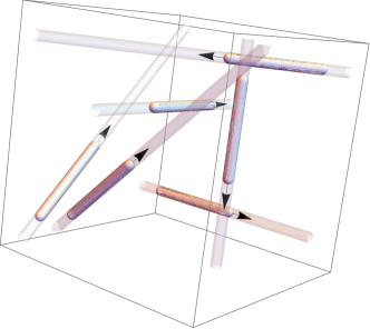
Figure 10: The intermittent jets in one of the $(\nicefrac{{\mathbb{T}}}{{r_{\perp}\lambda}})^{3}$ periodic boxes.

Lastly, we note that the intermittent jets $W_{(\xi)}$ are not divergence free, however assuming $r_{\perp}\ll r_{\|}$ they may be corrected by a small term, such that the sum with the corrector is divergence free. To see this, let us define $V_{(\xi)}:\mathbb{T}^{3}\times\mathbb{R}\rightarrow\mathbb{R}^{3}$ by

$$V_{(\xi)}(x,t):=V_{\xi,r_{\perp},r_{\|},\lambda,\mu}(x,t):=\frac{1}{n_{*}^{2}\lambda^{2}}\xi\,\psi_{(\xi)}(x,t)\,\Phi_{(\xi)}(x)\,,$$

where we still use the notation from (7.19). A computation then shows that

$$\mathrm{curl\,}\mathrm{curl\,}V_{(\xi)}-W_{(\xi)}=\underbrace{\frac{1}{n_{*}^{2}\lambda^{2}}\mathrm{curl\,}\left(\Phi_{(\xi)}\mathrm{curl\,}\left(\psi_{(\xi)}\xi\right)\right)}_{\equiv 0}+\frac{1}{n_{*}^{2}\lambda^{2}}\nabla\psi_{(\xi)}\times\mathrm{curl\,}\left(\Phi_{(\xi)}\xi\right)=:W_{(\xi)}^{(c)}\,.$$ (7.24)

Thus, by the definition of $W_{(\xi)}^{(c)}$, we have

$$\mathrm{div\,}\left(W_{(\xi)}+W^{(c)}_{(\xi)}\right)\equiv 0\,.$$

Moreover, since we have $r_{\perp}\ll r_{\|}$ the correction $W^{(c)}_{(\xi)}$ is comparatively small (say in $L^{2}$) compared to $W_{(\xi)}$. This follows from the estimates obeyed by the first two terms on the left side of (7.27).

Having established the important geometric properties of the intermittent jets, namely (7.22) and (7.23), we summarize the bounds obeyed by the intermittent jets, their incompressibility correctors, and their corresponding building blocks. By construction we have that the directions of oscillation for the functions defined in (7.19) are orthogonal. Therefore, we may use Fubini to combine the estimates obeyed by $\psi_{(\xi)}$ (which is a 1D function) and $\phi_{(\xi)},\Phi_{(\xi)}$ (which are 2D functions), to obtain estimates for the 3D functions $W_{(\xi)}$ and $V_{(\xi)}$. We claim that for $N,M\geq 0$ and $p\in[1,\infty]$ the following bounds hold:

$$\left\|\nabla^{N}\partial_{t}^{M}\psi_{(\xi)}\right\|_{L^{p}} \lesssim r_{\|}^{\nicefrac{{1}}{{p}}-\nicefrac{{1}}{{2}}}\left(\frac{r_{\perp}\lambda}{r_{\|}}\right)^{\!\!N}\left(\frac{r_{\perp}\lambda\mu}{r_{\|}}\right)^{\!\!M}$$ (7.25)

$$\left\|\nabla^{N}\phi_{(\xi)}\right\|_{L^{p}}+\left\|\nabla^{N}\Phi_{(\xi)}\right\|_{L^{p}} \lesssim r_{\perp}^{\nicefrac{{2}}{{p}}-1}\lambda^{N}$$ (7.26)

$$\left\|\nabla^{N}\partial_{t}^{M}W_{(\xi)}\right\|_{L^{p}}+\frac{r_{\|}}{r_{\perp}}\left\|\nabla^{N}\partial_{t}^{M}W_{(\xi)}^{(c)}\right\|_{L^{p}}+\lambda^{2}\left\|\nabla^{N}\partial_{t}^{M}V_{(\xi)}\right\|_{L^{p}} \lesssim r_{\perp}^{\nicefrac{{2}}{{p}}-1}r_{\|}^{\nicefrac{{1}}{{p}}-\nicefrac{{1}}{{2}}}\lambda^{N}\left(\frac{r_{\perp}\lambda\mu}{r_{\|}}\right)^{\!\!M}$$ (7.27)

where implicit constants may depend on $p$, $N$ and $M$, but are independent of $\lambda$, $r_{\perp}$, $r_{\|}$, $\mu$. For $N,M=0$, the corresponding $L^{p}$ estimates follow directly from simple scaling arguments and the bounds implied by (7.18) on the unit periodic box. For the derivative estimates we have assumed that

$$r_{\|}^{-1}\ll r_{\perp}^{-1}\ll\lambda\,$$

holds, in order to identify the largest frequency of oscillation.

7.5 The perturbation

In this section we will construct the perturbation $w_{q+1}$ which defines $v_{q+1}=v_{\ell}+w_{q+1}$.

7.5.1 Parameter choices

In Section 7.4 above, we have worked with abstract parameters $\lambda,\mu,r_{\perp}$, and $r_{\|}$. They had to obey the heuristic bounds $\lambda^{-1}\ll r_{\perp}\ll r_{\|}\ll 1$, and $\lambda r_{\perp}$ had to be a natural number. It is convenient to now fix these parameters, all in terms of $\lambda_{q+1}$. At this stage in the proof not all these choices are motivated, and some of the choices only become justified based on arguments in Section 7.6 below. However, in order to specify the bounds on the velocity increment $w_{q+1}$, and the new velocity $v_{q+1}$, it is convenient to specify these parameters at this stage already.

Recall that $\lambda_{q}$ is defined in (7.1) as $2\pi a^{(b^{q})}$. We define

$$r_{\|} =\lambda_{q+1}^{-\nicefrac{{4}}{{7}}}$$ (7.28a)

$$r_{\perp} =r_{\|}^{-\nicefrac{{1}}{{4}}}\lambda_{q+1}^{-1}(2\pi)^{-\nicefrac{{1}}{{7}}}=\lambda_{q+1}^{-\nicefrac{{6}}{{7}}}(2\pi)^{-\nicefrac{{1}}{{7}}}$$ (7.28b)

$$\mu =\lambda_{q+1}r_{\|}r_{\perp}^{-1}=\lambda_{q+1}^{\nicefrac{{9}}{{7}}}(2\pi)^{\nicefrac{{1}}{{7}}}$$ (7.28c)

In (7.28b) we have introduced a strange power of $2\pi$ in order to ensure that

$$\lambda_{q+1}r_{\perp}=((2\pi)^{-1}\lambda_{q+1})^{\nicefrac{{1}}{{7}}}=a^{\nicefrac{{(b^{q+1})}}{{7}}}\in\mathbb{N}\,,$$

which ensures the correct periodicity of $W_{(\xi)}$, $V_{(\xi)}$, $\Phi_{(\xi)}$, $\phi_{(\xi)}$ and $\psi_{(\xi)}$. For this purpose, it is sufficient to ensure that $b$ is a multiple of $7$. For the remainder of the Navier-Stokes section we use these fixed choices of $\lambda,r_{\perp},r_{\|}$, and $\mu$, for the short hand notation $W_{(\xi)}$, $V_{(\xi)}$, $\Phi_{(\xi)}$, $\phi_{(\xi)}$ and $\psi_{(\xi)}$ introduced in Section 7.4. We also recall that the parameter $\ell$ was chosen to obey (7.10) above.

7.5.2 Amplitudes

Let $\chi$ be a smooth function such that

$$\chi(z)=\begin{cases}1&\mbox{if}\quad 0\leq z\leq 1\\ z&\mbox{if}\quad z\geq 2\end{cases}$$

and with $z\leq 2\chi(z)\leq 4z$ for $z\in(1,2)$. For such a function $\chi$ we then define

$$\rho(x,t)=4c_{R}\delta_{q+1}\chi\left((c_{R}\delta_{q+1})^{-1}\left|\mathring{R}_{\ell}(x,t)\right|\right)\,.$$

This simplified definition of $\rho$ was introduced in [138]. The main properties of $\rho$ are that pointwise in $(x,t)$ we have

$$\left|\frac{\mathring{R}_{\ell}(x,t)}{\rho(x,t)}\right|=\frac{1}{4}\frac{(c_{R}\delta_{q+1})^{-1}|\mathring{R}_{\ell}(x,t)|}{\chi((c_{R}\delta_{q+1})^{-1}|\mathring{R}_{\ell}(x,t)|)}\leq\frac{1}{2}$$ (7.29)

and moreover for any $p\in[1,\infty]$ we have

$$\left\|\rho\right\|_{L^{p}}\leq 16\left(c_{R}(8\pi^{3})^{\nicefrac{{1}}{{p}}}\delta_{q+1}+\left\|\mathring{R}_{\ell}\right\|_{L^{p}}\right)$$ (7.30)

Moreover, using the Sobolev embedding $W^{4,1}\subset C^{0}$, from (7.2c), standard mollification estimates and repeated applications of the chain rule (see e.g. [16, Proposition C.1]), we obtain that

$$\left\|\rho\right\|_{C^{N}_{x,t}}\lesssim\delta_{q+1}\ell^{-4}\ell^{-5N}\lesssim\ell^{-4-5N}$$ (7.31)

for any $N\geq 0$, where the implicit constant depends on $N$.

Next we define the amplitude functions

$$a_{(\xi)}(x,t):=a_{\xi,q+1}(x,t):=\;\rho(x,t)^{\nicefrac{{1}}{{2}}}\;\gamma_{\xi}\left(\mathrm{Id}-\frac{\mathring{R}_{\ell}(x,t)}{\rho(x,t)}\right)\,.$$ (7.32)

In view of (7.29), the matrix $\mathrm{Id}-\rho^{-1}\mathring{R}_{\ell}$ lies in the domain of definition of the functions $\gamma_{\xi}$ from Lemma 6.6. We note that as a consequence of (7.22), (7.32), and of Lemma  6.6, we have

$$\sum_{\xi\in\Lambda}a_{(\xi)}^{2}\fint_{\mathbb{T}^{3}}W_{(\xi)}\otimes W_{(\xi)}dx=\rho\,\mathrm{Id}-\mathring{R}_{\ell}\,,$$ (7.33)

which justifies the definition of the amplitude functions $a_{(\xi)}$.

The amplitudes $a_{(\xi)}$ have a good $L^{2}$ norm. Indeed, using (7.30), the bound (7.2c), the fact that the mollifier has mass $1$, the definition of the constant $M$ in Lemma 6.6, and choosing the constant $C_{\gamma}$ as discussed in the first paragraph of Section 7.4, we obtain

$$\left\|a_{(\xi)}\right\|_{L^{2}}\leq\left\|\rho\right\|_{L^{1}}^{\nicefrac{{1}}{{2}}}\left\|\gamma_{\xi}\right\|_{C^{0}(B_{\nicefrac{{1}}{{2}}}(\mathrm{Id}))}\leq\frac{4c_{R}^{\nicefrac{{1}}{{2}}}\left((8\pi^{3})+1\right)^{\nicefrac{{1}}{{2}}}M}{8|\Lambda|((8\pi^{3})+1)^{\nicefrac{{1}}{{2}}}}\delta_{q+1}^{\nicefrac{{1}}{{2}}}\leq\frac{\delta_{q+1}^{\nicefrac{{1}}{{2}}}}{2|\Lambda|}$$ (7.34)

by choosing $c_{R}$ sufficiently small, in terms of the universal constants $M$ and $|\Lambda|$. Lastly, we note that since $\rho$ is bounded from below by $4c_{R}\delta_{q+1}$, using the chain rule and standard mollification estimates, similarly to (7.31), we have

$$\left\|a_{(\xi)}\right\|_{C^{N}_{x,t}}\lesssim\delta_{q+1}^{\nicefrac{{1}}{{2}}}\ell^{-2}\ell^{-5N}\lesssim\ell^{-2-5N}$$ (7.35)

for all $N\geq 0$.

7.5.3 Principal part of the perturbation, incompressibility and temporal correctors

The principal part of $w_{q+1}$ is defined as

$$w^{(p)}_{q+1}:=\sum_{\xi\in\Lambda}a_{(\xi)}\;W_{(\xi)}\,.$$ (7.36)

Note that in view of (7.21) we have that the summands in (7.36) have mutually disjoint supports. Also, by (7.33) we have that the low-frequency part of $w_{q+1}^{(p)}\otimes w_{q+1}^{(p)}$ cancels the mollification stress $\mathring{R}_{\ell}$. More precisely, we have

$$w_{q+1}^{(p)}\otimes w_{q+1}^{(p)}+\mathring{R}_{\ell}=\sum_{\xi\in\Lambda}a_{(\xi)}^{2}\mathbb{P}_{\neq 0}\left(W_{(\xi)}\otimes W_{(\xi)}\right)+\rho\mathrm{Id}\,.$$ (7.37)

In order to fix the fact that $w_{q+1}^{(p)}$ is not divergence free, we define an incompressibility corrector by

$$w^{(c)}_{q+1} :=\sum_{\xi\in\Lambda}\mathrm{curl\,}\left(\nabla a_{(\xi)}\times V_{(\xi)}\right)+\nabla a_{(\xi)}\times\mathrm{curl\,}V_{(\xi)}+a_{(\xi)}W_{(\xi)}^{(c)}\,.$$ (7.38)

The above definition is motivated by a computation similar to (7.24), which guarantees that

$$w_{q+1}^{(p)}+w_{q+1}^{(c)}=\sum_{\xi\in\Lambda}\mathrm{curl\,}\mathrm{curl\,}(a_{(\xi)}V_{(\xi)})\,,$$ (7.39)

and thus ensures

$$\mathrm{div\,}\left(w_{q+1}^{(p)}+w_{q+1}^{(c)}\right)\equiv 0\,.$$

In addition to the incompressibility corrector $w_{q+1}^{(c)}$, we introduce a temporal corrector $w_{q+1}^{(t)}$, which is defined by

$$w^{(t)}_{q+1}:=-\frac{1}{\mu}\sum_{\xi\in\Lambda}\mathbb{P}_{H}\mathbb{P}_{\neq 0}\left(a_{(\xi)}^{2}\phi^{2}_{(\xi)}\psi^{2}_{(\xi)}\xi\right)\,,$$ (7.40)

where as before $\mathbb{P}_{H}$ is the Helmholtz-Leray projector. By construction, $\mathrm{div\,}w_{q+1}^{(t)}=0$, and the choice of $\mu$ ensures that this corrector is much smaller than the principal corrector $w_{q+1}^{(p)}$. The purpose of introducing the temporal corrector only becomes apparent when considering the oscillation error in Section 7.6. More precisely, we use the key identity (7.23) obeyed by the intermittent jets, and the fact that $\mathrm{Id}-\mathbb{P}_{H}=\nabla\Delta^{-1}\mathrm{div\,}$, to rewrite

$$\partial_{t}w_{q+1}^{(t)}+\sum_{\xi\in\Lambda}\mathbb{P}_{\neq 0}\left(a_{(\xi)}^{2}\mathrm{div\,}\left(W_{(\xi)}\otimes W_{(\xi)}\right)\right)$$

$$\quad=-\frac{1}{\mu}\sum_{\xi\in\Lambda}\mathbb{P}_{H}\mathbb{P}_{\neq 0}\partial_{t}\left(a_{(\xi)}^{2}\phi^{2}_{(\xi)}\psi^{2}_{(\xi)}\xi\right)+\frac{1}{\mu}\sum_{\xi\in\Lambda}\mathbb{P}_{\neq 0}\left(a_{(\xi)}^{2}\partial_{t}\left(\phi^{2}_{(\xi)}\psi^{2}_{(\xi)}\xi\right)\right)$$

$$\quad=\underbrace{(\mathrm{Id}-\mathbb{P}_{H})\frac{1}{\mu}\sum_{\xi\in\Lambda}\mathbb{P}_{\neq 0}\partial_{t}\left(a_{(\xi)}^{2}\phi^{2}_{(\xi)}\psi^{2}_{(\xi)}\xi\right)}_{=:\nabla P}-\frac{1}{\mu}\sum_{\xi\in\Lambda}\mathbb{P}_{\neq 0}\left(\partial_{t}a_{(\xi)}^{2}\left(\phi^{2}_{(\xi)}\psi^{2}_{(\xi)}\xi\right)\right)\,.$$ (7.41)

Identity (7.41) shows the essential role played by temporal oscillations in our construction.

7.5.4 The velocity increment and verification of the inductive estimates

The total velocity increment $w_{q+1}$ is defined by

$$w_{q+1}:=w_{q+1}^{(p)}+w_{q+1}^{(c)}+w_{q+1}^{(t)}\,,$$ (7.42)

and is by construction mean zero and divergence-free. The new velocity field $v_{q+1}$ is defined as

$$v_{q+1}=v_{q}+w_{q+1}\,.$$ (7.43)

In this section we verify that the inductive estimates (7.2a), (7.2b) hold with $q$ replaced by $q+1$, and that (7.3) is satisfied.

In order to efficiently estimate the $L^{2}$ norm of the principal part of the perturbation $w_{q+1}^{(p)}$ we need to use the fact that the amplitudes $a_{(\xi)}$ oscillate at a much lower frequency than the intermittent jets $W_{(\xi)}$. For this purpose, we recall the $L^{p}$ de-correlation estimate [20, Lemma 3.6]:

Lemma 7.4.

Fix integers $N,\kappa\geq 1$ and let $\zeta>1$ be such that

$$\frac{2\pi\sqrt{3}\zeta}{\kappa}\leq\frac{1}{3}\qquad\mbox{and}\qquad\zeta^{4}\frac{(2\pi\sqrt{3}\zeta)^{N}}{\kappa^{N}}\leq 1\,.$$ (7.44)

Let $p\in\{1,2\}$, and let $f$ be a $\mathbb{T}^{3}$-periodic function such that there exists a constant $C_{f}>0$ such that

$$\|D^{j}f\|_{L^{p}}\leq C_{f}\zeta^{j}\,,$$

holds for all $0\leq j\leq N+4$. In addition, let $g$ be a $(\nicefrac{{\mathbb{T}}}{{\kappa}})^{3}$-periodic function. Then we have that

$$\|fg\|_{L^{p}}\lesssim C_{f}\|g\|_{L^{p}}\,,$$

where the implicit constant is universal.

We wish to apply the above de-correlation Lemma 7.4 in $L^{2}$ with $f=a_{(\xi)}$ and $g=W_{(\xi)}$, which is by construction $(\mathbb{T}/\kappa)^{3}$ periodic with $\kappa=\lambda_{q+1}r_{\perp}$. For this purpose, note that by (7.34) and (7.35) we obtain that

$$\left\|D^{j}a_{(\xi)}\right\|_{L^{2}}\leq\frac{1}{2|\Lambda|}\delta_{q+1}^{\nicefrac{{1}}{{2}}}\ell^{-8j}\,,$$

and thus we can take $C_{f}=\frac{1}{2|\Lambda|}\delta_{q+1}^{\nicefrac{{1}}{{2}}}$ and $\zeta=\ell^{-8}$. Since by (7.10) we have $\zeta\leq\lambda_{q+1}^{16\alpha}$, whereas by (7.28b) we have that $\lambda_{q+1}r_{\perp}\approx\lambda_{q+1}^{\nicefrac{{1}}{{7}}}$. Thus, since $\alpha$ is sufficiently small, condition (7.44) is satisfied for any $N\geq 1$, and thus Lemma 7.4 is applicable. Combining the resulting estimate with the normalization of $W_{(\xi)}$ as $\left\|W_{(\xi)}\right\|_{L^{2}}=1$, we obtain

$$\left\|w_{q+1}^{(p)}\right\|_{L^{2}}\leq\sum_{\xi\in\Lambda}\frac{2}{2|\Lambda|}\delta_{q+1}^{\nicefrac{{1}}{{2}}}\left\|W_{(\xi)}\right\|_{L^{2}}\leq\frac{1}{2}\delta_{q+1}^{\nicefrac{{1}}{{2}}}.$$ (7.45)

For the correctors $w_{q+1}^{(c)}$ and $w_{q+1}^{(t)}$, and for bounds on the other $L^{p}$ norms of $w_{q+1}^{(p)}$ we may afford slightly less precise bounds (which do not appeal to Lemma 7.4), which follow directly from (7.27), (7.35), and the parameter choices in (7.28):

$$\left\|w_{q+1}^{(p)}\right\|_{L^{p}} \lesssim\sum_{\xi\in\Lambda}\left\|a_{(\xi)}\right\|_{C^{0}}\left\|W_{(\xi)}\right\|_{L^{p}}$$

$$\qquad\lesssim\delta_{q+1}^{\nicefrac{{1}}{{2}}}\ell^{-2}r_{\perp}^{\nicefrac{{2}}{{p}}-1}r_{\|}^{\nicefrac{{1}}{{p}}-\nicefrac{{1}}{{2}}}$$ (7.46a)

$$\left\|w_{q+1}^{(c)}\right\|_{L^{p}} \lesssim\sum_{\xi\in\Lambda}\left\|a_{(\xi)}\right\|_{C^{0}}\left\|W_{(\xi)}^{(c)}\right\|_{L^{p}}+\left\|a_{(\xi)}\right\|_{C^{2}}\left\|V_{(\xi)}\right\|_{W^{1,p}}$$

$$\qquad\lesssim\delta_{q+1}^{\nicefrac{{1}}{{2}}}\ell^{-12}r_{\perp}^{\nicefrac{{2}}{{p}}-1}r_{\|}^{\nicefrac{{1}}{{p}}-\nicefrac{{1}}{{2}}}\left(r_{\perp}r_{\|}^{-1}+\lambda_{q+1}^{-1}\right)\lesssim\delta_{q+1}^{\nicefrac{{1}}{{2}}}\ell^{-12}r_{\perp}^{\nicefrac{{2}}{{p}}}r_{\|}^{\nicefrac{{1}}{{p}}-\nicefrac{{3}}{{2}}}$$ (7.46b)

$$\left\|w_{q+1}^{(t)}\right\|_{L^{p}} \lesssim\mu^{-1}\sum_{\xi\in\Lambda}\left\|a_{(\xi)}\right\|_{C^{0}}^{2}\left\|\phi_{(\xi)}\right\|_{L^{2p}}^{2}\left\|\psi_{(\xi)}\right\|_{L^{2p}}^{2}$$

$$\qquad\lesssim\delta_{q+1}\ell^{-4}r_{\perp}^{\nicefrac{{2}}{{p}}-1}r_{\|}^{\nicefrac{{1}}{{p}}-\nicefrac{{1}}{{2}}}(\mu^{-1}r_{\perp}^{-1}r_{\|}^{-\nicefrac{{1}}{{2}}})\lesssim\delta_{q+1}\ell^{-4}r_{\perp}^{\nicefrac{{2}}{{p}}-1}r_{\|}^{\nicefrac{{1}}{{p}}-2}\lambda_{q+1}^{-1}.$$ (7.46c)

Combining (7.45) with the last two estimates of (7.46) for $p=2$, and using the parameter choices (7.28), we obtain that for a sufficiently large constant $C$ (which is independent of $q$), we have

$$\left\|w_{q+1}\right\|_{L^{2}} \leq\delta_{q+1}^{\nicefrac{{1}}{{2}}}\left(\frac{1}{2}+C\ell^{-12}r_{\perp}r_{\|}^{-1}+C\ell^{-4}r_{\|}^{-\nicefrac{{3}}{{2}}}\lambda_{q+1}^{-1}\right)$$

$$\leq\delta_{q+1}^{\nicefrac{{1}}{{2}}}\left(\frac{1}{2}+C\lambda_{q+1}^{24\alpha-\nicefrac{{2}}{{7}}}+C\lambda_{q+1}^{8\alpha-\nicefrac{{1}}{{7}}}\right)\leq\frac{3}{4}\delta_{q+1}^{\nicefrac{{1}}{{2}}}\,.$$ (7.47)

In the last inequality we have used that $\alpha$ is sufficiently small, that $\beta$ is sufficiently small in terms of $\alpha$, and that by letting $a$ be sufficiently large we have $C\lambda_{q+1}^{-\nicefrac{{1}}{{10}}}\leq\nicefrac{{1}}{{8}}$. Moreover, from (7.13) we have that

$$\left\|v_{q}-v_{\ell}\right\|_{L^{2}}\lesssim\lambda_{q+1}^{-\alpha}\leq\lambda_{q+1}^{-\nicefrac{{\alpha}}{{2}}}\leq\frac{1}{4}\delta_{q+1}^{\nicefrac{{1}}{{2}}}$$ (7.48)

once we ensure that $\beta$ is sufficiently small, in terms of $\alpha$, and we take $a$ to be sufficiently large. Combining (7.47) and (7.48) we obtain that

$$\left\|v_{q+1}-v_{q}\right\|_{L^{2}}\leq\left\|w_{q+1}\right\|_{L^{2}}+\left\|v_{\ell}-v_{q}\right\|_{L^{2}}\leq\delta_{q+1}^{\nicefrac{{1}}{{2}}},$$

and thus (7.3) is satisfied.

The bound (7.2a) at level $q+1$ follows from (7.14), (7.47), and the inequality $-\delta_{q}^{\nicefrac{{1}}{{2}}}+\delta_{q+1}^{\nicefrac{{1}}{{2}}}\leq-\delta_{q+1}^{\nicefrac{{1}}{{2}}}$. The latter simply requires that $a$ is taken sufficiently large.

In addition, taking either a spatial or a temporal derivative, using the bounds (7.25)–(7.27), the estimate for $\ell^{-1}$ in (7.10), and the parameter choices (7.28) we may prove

$$\left\|w_{q+1}^{(p)}\right\|_{C^{1}_{x,t}} \lesssim\ell^{-7}r_{\perp}^{-1}r_{\|}^{-\nicefrac{{1}}{{2}}}\lambda_{q+1}\left(1+\frac{r_{\perp}\mu}{r_{\|}}\right)\lesssim\ell^{-7}r_{\perp}^{-1}r_{\|}^{-\nicefrac{{1}}{{2}}}\lambda_{q+1}^{2}$$ (7.49a)

$$\left\|w_{q+1}^{(c)}\right\|_{C^{1}_{x,t}} \lesssim\ell^{-17}r_{\|}^{-\nicefrac{{3}}{{2}}}\lambda_{q+1}\left(1+\frac{r_{\perp}\mu}{r_{\|}}\right)\lesssim\ell^{-17}r_{\|}^{-\nicefrac{{3}}{{2}}}\lambda_{q+1}^{2}$$ (7.49b)

$$\left\|w_{q+1}^{(t)}\right\|_{C^{1}_{x,t}} \lesssim\ell^{-9}r_{\perp}^{-1}r_{\|}^{-2}\lambda_{q+1}^{-1}\lambda_{q+1}^{1+\alpha}\left(1+\frac{r_{\perp}\mu}{r_{\|}}\right)\lesssim\ell^{-9}r_{\perp}^{-1}r_{\|}^{-2}\lambda_{q+1}^{1+\alpha}\,.$$ (7.49c)

In the last inequality we have paid an extra power of $\lambda_{q+1}^{\alpha}$ because $\mathbb{P}_{H}\mathbb{P}_{\neq 0}$ is not a bounded operator on $C^{0}$. Combining the $C^{1}_{x,t}$ estimate for $v_{\ell}$ with the above obtained bound (7.15), we obtain from (7.43) that

$$\left\|v_{q+1}\right\|_{C^{1}_{x,t}}\lesssim\left\|v_{\ell}\right\|_{C^{1}_{x,t}}+\left\|w_{q+1}\right\|_{C^{1}_{x,t}} \lesssim\lambda_{q+1}^{\alpha}+\lambda_{q+1}^{14\alpha+\nicefrac{{22}}{{7}}}+\lambda_{q+1}^{34\alpha+\nicefrac{{20}}{{7}}}+\lambda_{q+1}^{19\alpha+3}$$

$$\leq\lambda_{q+1}^{2\alpha}+\lambda_{q+1}^{35\alpha+\nicefrac{{22}}{{7}}}\leq\lambda_{q+1}^{4}$$

once we take $\alpha$ to be sufficiently small. This proves (7.2b) at level $q+1$.

7.6 Reynolds stress

7.6.1 Decomposition of the new Reynolds stress

Recall that $v_{q+1}=w_{q+1}+v_{\ell}$, where $v_{\ell}$ is defined in Section 7.3. Subtracting from (4.7) at level $q+1$ the system (7.8), we thus obtain (compare to (5.41) in the case of Euler)

$$\mathrm{div\,}\mathring{R}_{q+1}-\nabla p_{q+1} =\underbrace{-\nu\Delta w_{q+1}+\partial_{t}(w^{(p)}_{q+1}+w^{(c)}_{q+1})+\mathrm{div\,}(v_{\ell}\otimes w_{q+1}+w_{q+1}\otimes v_{\ell})}_{\mathrm{div\,}(R_{\rm linear})+\nabla p_{\rm linear}}$$

$$\qquad+\underbrace{\mathrm{div\,}\left((w_{q+1}^{(c)}+w_{q+1}^{(t)})\otimes w_{q+1}+w_{q+1}^{(p)}\otimes(w_{q+1}^{(c)}+w_{q+1}^{(t)})\right)}_{\mathrm{div\,}(R_{\rm corrector})+\nabla p_{\rm corrector}}$$

$$\qquad+\underbrace{\mathrm{div\,}(w_{q+1}^{(p)}\otimes w_{q+1}^{(p)}+\mathring{R}_{\ell})+\partial_{t}w^{(t)}_{q+1}}_{\mathrm{div\,}(R_{\rm oscillation})+\nabla p_{\rm oscillation}}+\,\mathrm{div\,}(R_{\rm commutator})-\nabla p_{\ell}\,.$$ (7.50)

Here $R_{\rm commutator}$ is as defined in (7.9) and we have used the inverse divergence operator from (5.37) to define

$$R_{\rm linear} =-\nu\mathcal{R}\Delta w_{q+1}+\mathcal{R}\partial_{t}(w_{q+1}^{(p)}+w_{q+1}^{(c)})+v_{\ell}\mathring{\otimes}w_{q+1}+w_{q+1}\mathring{\otimes}v_{\ell}$$ (7.51)

$$R_{\rm corrector} =(w_{q+1}^{(c)}+w_{q+1}^{(t)})\mathring{\otimes}w_{q+1}+w_{q+1}^{(p)}\mathring{\otimes}(w_{q+1}^{(c)}+w_{q+1}^{(t)})$$ (7.52)

where $p_{\rm linear}=2v_{\ell}\cdot w_{q+1}$ and $p_{\rm corrector}=|w_{q+1}|^{2}-|w_{q+1}^{(p)}|^{2}$. The remaining stress $R_{\rm oscillation}$ and corresponding pressure $p_{\rm oscillation}$ are defined as follows. By (7.37) and (7.41) we have that

$$\mathrm{div\,}(w_{q+1}^{(p)}\otimes w_{q+1}^{(p)}+\mathring{R}_{\ell})+\partial_{t}w^{(t)}_{q+1}$$

$$\qquad=\sum_{\xi\in\Lambda}\mathrm{div\,}\left(a_{(\xi)}^{2}\mathbb{P}_{\neq 0}\left(W_{(\xi)}\otimes W_{(\xi)}\right)\right)+\nabla\rho+\partial_{t}w^{(t)}_{q+1}$$

$$\qquad=\sum_{\xi\in\Lambda}\mathbb{P}_{\neq 0}\left(\nabla a_{(\xi)}^{2}\mathbb{P}_{\neq 0}\left(W_{(\xi)}\otimes W_{(\xi)}\right)\right)+\nabla\rho+\sum_{\xi\in\Lambda}\mathbb{P}_{\neq 0}\left(a_{(\xi)}^{2}\mathrm{div\,}\left(W_{(\xi)}\otimes W_{(\xi)}\right)\right)+\partial_{t}w^{(t)}_{q+1}$$

$$\qquad=\sum_{\xi\in\Lambda}\mathbb{P}_{\neq 0}\left(\nabla a_{(\xi)}^{2}\mathbb{P}_{\neq 0}\left(W_{(\xi)}\otimes W_{(\xi)}\right)\right)+\nabla\rho+\nabla P-\frac{1}{\mu}\sum_{\xi\in\Lambda}\mathbb{P}_{\neq 0}\left(\partial_{t}a_{(\xi)}^{2}\left(\phi^{2}_{(\xi)}\psi^{2}_{(\xi)}\xi\right)\right)\,,$$

where the pressure term $P$ is as defined by the first term on the right side of (7.41). Therefore, we define $p_{\rm oscillation}=\rho+P$, and let

$$R_{\rm oscillation} =\sum_{\xi\in\Lambda}\mathcal{R}\left(\nabla a_{(\xi)}^{2}\mathbb{P}_{\neq 0}\left(W_{(\xi)}\otimes W_{(\xi)}\right)\right)-\frac{1}{\mu}\sum_{\xi\in\Lambda}\mathcal{R}\left(\partial_{t}a_{(\xi)}^{2}\left(\phi^{2}_{(\xi)}\psi^{2}_{(\xi)}\xi\right)\right)\,.$$ (7.53)

(We recall there that $\mathcal{R}=\mathcal{R}\mathbb{P}_{\neq 0}$.) Now all the terms in (7.50) are well defined. We have $p_{q+1}=p_{\ell}-p_{\rm oscillation}-p_{\rm corrector}-p_{\rm linear}$ and

$$\mathring{R}_{q+1}=R_{\rm linear}+R_{\rm corrector}+R_{\rm oscillation}+R_{\rm commutator}\,$$ (7.54)

which are stresses defined in (7.51), (7.52), (7.53), and respectively (7.9).

7.6.2 Estimates for the new Reynolds stress

We need to estimate the new stress $\mathring{R}_{q+1}$ in $L^{1}$. However, Calderón-Zygmund operators such as $\nabla\mathcal{R}$ just fail to be bounded on $L^{1}$. For this purpose, we introduce an integrability parameter

$$p\in(1,2]\,\qquad\mbox{such that}\qquad p-1\ll 1.$$ (7.55)

We may now use that Calderón-Zygmund operators are bounded on $L^{p}$. Recalling (7.28), we fix $p$ to obey

$$r_{\perp}^{\nicefrac{{2(1-p)}}{{p}}}r_{\|}^{\nicefrac{{(1-p)}}{{p}}}\leq(2\pi)^{\nicefrac{{1}}{{7}}}\lambda_{q+1}^{\nicefrac{{16(p-1)}}{{(7p)}}}\leq\lambda_{q+1}^{\alpha}$$ (7.56)

where $0<\alpha\ll 1$ is as in Remark 7.3. For instance, we may take $p=\nicefrac{{32}}{{(32-7\alpha)}}>1$.

Linear error.   Recalling identity (7.39), using that $\nu\in(0,1]$, that $\mathcal{R}\mathrm{curl\,}$ is a bounded operator on $L^{p}$, and appealing to the Sobolev embedding $H^{3}\subset C^{0}$, the linear stress defined in (7.51) obeys

$$\left\|R_{\rm linear}\right\|_{L^{p}} \lesssim\nu\left\|\mathcal{R}\Delta w_{q+1}\right\|_{L^{p}}+\left\|v_{\ell}\mathring{\otimes}w_{q+1}+w_{q+1}\mathring{\otimes}v_{\ell}\right\|_{L^{p}}+\left\|\mathcal{R}\partial_{t}(w^{(p)}_{q+1}+w^{(c)}_{q+1})\right\|_{L^{p}}$$

$$\lesssim\left\|\nabla w_{q+1}\right\|_{L^{p}}+\left\|v_{\ell}\right\|_{L^{\infty}}\left\|w_{q+1}\right\|_{L^{p}}+\sum_{\xi\in\Lambda}\left\|\partial_{t}\mathrm{curl\,}(a_{(\xi)}V_{(\xi)})\right\|_{L^{p}}$$

$$\lesssim(1+\left\|v_{\ell}\right\|_{C^{1}})\sum_{\xi\in\Lambda}\left\|a_{(\xi)}\right\|_{C^{1}}\left\|W_{(\xi)}\right\|_{W^{1,p}}$$

$$\qquad+\sum_{\xi\in\Lambda}\left(\left\|a_{(\xi)}\right\|_{C^{1}}\left\|\partial_{t}V_{(\xi)}\right\|_{W^{1,p}}+\left\|\partial_{t}a_{(\xi)}\right\|_{C^{1}}\left\|V_{(\xi)}\right\|_{W^{1,p}}\right)\,.$$

By appealing to (7.15), (7.27), (7.35), and (7.56) we obtain from the above estimate that

$$\left\|R_{\rm linear}\right\|_{L^{p}} \lesssim\ell^{-8}r_{\perp}^{\nicefrac{{2}}{{p}}-1}r_{\|}^{\nicefrac{{1}}{{p}}-\nicefrac{{1}}{{2}}}\lambda_{q+1}+\ell^{-7}r_{\perp}^{\nicefrac{{2}}{{p}}}r_{\|}^{\nicefrac{{1}}{{p}}-\nicefrac{{3}}{{2}}}\mu+\ell^{-12}r_{\perp}^{\nicefrac{{2}}{{p}}-1}r_{\|}^{\nicefrac{{1}}{{p}}-\nicefrac{{1}}{{2}}}\lambda_{q+1}^{-1}$$

$$\lesssim\ell^{-12}r_{\perp}^{\nicefrac{{2(1-p)}}{{p}}}r_{\|}^{\nicefrac{{(1-p)}}{{p}}}\left(r_{\perp}r_{\|}^{\nicefrac{{1}}{{2}}}\lambda_{q+1}+r_{\perp}^{2}r_{\|}^{-\nicefrac{{1}}{{2}}}\mu\right)$$

$$\lesssim\ell^{-12}\lambda_{q+1}^{\alpha}\left(r_{\perp}r_{\|}^{\nicefrac{{1}}{{2}}}\lambda_{q+1}+r_{\perp}^{2}r_{\|}^{-\nicefrac{{1}}{{2}}}\mu\right)\,.$$ (7.57)

Corrector error.   Recall the definitions (7.36), (7.38), (7.40), and the estimates (7.46). From the parameter choices in (7.28), we see that the worse $L^{2p}$ estimate is the one for for the principal corrector.

Therefore, using that $\delta_{q+1}\leq 1$, from the parameter inequalities (7.46) is used, and the choice of $p$ in (7.56), it follows that the corrector stress defined in (7.52) obeys

$$\left\|R_{\rm corrector}\right\|_{L^{p}} \leq\left\|w_{q+1}^{(c)}+w_{q+1}^{(t)}\right\|_{L^{2p}}\left\|w_{q+1}\right\|_{L^{2p}}+\left\|w_{q+1}^{(p)}\right\|_{L^{2p}}\left\|w_{q+1}^{(c)}+w_{q+1}^{(t)}\right\|_{L^{2p}}$$

$$\lesssim\left(\ell^{-12}r_{\perp}^{\nicefrac{{1}}{{p}}}r_{\|}^{\nicefrac{{1}}{{2p}}-\nicefrac{{3}}{{2}}}+\ell^{-4}\lambda_{q+1}^{-1}r_{\perp}^{\nicefrac{{1}}{{p}}-1}r_{\|}^{\nicefrac{{1}}{{2p}}-2}\right)\ell^{-2}r_{\perp}^{\nicefrac{{1}}{{p}}-1}r_{\|}^{\nicefrac{{1}}{{2p}}-\nicefrac{{1}}{{2}}}$$

$$\lesssim\ell^{-14}\lambda_{q+1}^{\alpha}\left(r_{\perp}r_{\|}^{-1}+\lambda_{q+1}^{-1}r_{\|}^{-\nicefrac{{3}}{{2}}}\right)\,.$$ (7.58)

Oscillation error.   The oscillation error defined in (7.53) has two terms, let us call $R_{\rm oscillation}^{(x)}$ the one when the spatial gradient lands on $a_{(\xi)}$ and let us denote by $R_{\rm oscillation}^{(t)}$ the one when temporal derivatives land on $a_{(\xi)}$.

Let us treat $R_{\rm oscillation}^{(x)}$ first. Note that by definition $W_{(\xi)}$ is $(\nicefrac{{\mathbb{T}}}{{r_{\perp}\lambda_{q+1}}})^{3}$ periodic. Therefore, so is $W_{(\xi)}\otimes W_{(\xi)}$ and we obtain that the minimal active frequency in $\mathbb{P}_{\neq 0}(W_{(\xi)}\otimes W_{(\xi)})$ is given by $r_{\perp}\lambda_{q+1}$. Equivalently, we have

$$\mathbb{P}_{\neq 0}(W_{(\xi)}\otimes W_{(\xi)})=\mathbb{P}_{\geq\nicefrac{{r_{\perp}\lambda_{q+1}}}{{2}}}(W_{(\xi)}\otimes W_{(\xi)}).$$

On the other hand, the amplitude term $\nabla a_{(\xi)}^{2}$ oscillates at a much lower frequency (proportional to $\ell^{-5}$), so that we expect the inverse divergence operator $\mathcal{R}$ to gain a factor of $r_{\perp}\lambda_{q+1}$. To make this intuition precise, let us recall [20, Lemma B.1].

Lemma 7.5.

Fix parameters $1\leq\zeta<\kappa$, $p\in(1,2]$, and assume there exists a $N\in\mathbb{N}$ such that

$$\zeta^{N}\leq\kappa^{N-2}\,.$$

Let $a\in C^{N}(\mathbb{T}^{3})$ be such that there exists $C_{a}>0$ with

$$\left\|D^{j}a\right\|_{C^{0}}\leq C_{a}\zeta^{j}$$ (7.59)

for all $0\leq j\leq N$. Assume furthermore that $f\in L^{p}(\mathbb{T}^{3})$ is such that $\int_{\mathbb{T}^{3}}a(x)\mathbb{P}_{\geq\kappa}f(x)dx=0$. Then we have

$$\left\||\nabla|^{-1}(a\;\mathbb{P}_{\geq\kappa}f)\right\|_{L^{p}}\lesssim C_{a}\frac{\left\|f\right\|_{L^{p}}}{\kappa}$$ (7.60)

where the implicit constant depends only on $p$ and $N$.

From (7.35) we see that $\nabla a_{(\xi)}^{2}$ obeys (7.59) with $C_{a}=\ell^{-9}$, and $\zeta=\ell^{-5}$. Since $\ell^{-5}\leq\lambda_{q+1}^{10\alpha}\ll\lambda_{q+1}^{\nicefrac{{1}}{{7}}}\approx r_{\perp}\lambda_{q+1}$, we are justified to use Lemma 7.5 (with any $N\geq 3$), combined with the bound (7.27), to conclude that

$$\left\|R_{\rm oscillation}^{(x)}\right\|_{L^{p}} \leq\sum_{\xi\in\Lambda}\left\|\mathcal{R}\left(\nabla a_{(\xi)}^{2}\mathbb{P}_{\geq\nicefrac{{r_{\perp}\lambda_{q+1}}}{{2}}}\left(W_{(\xi)}\otimes W_{(\xi)}\right)\right)\right\|_{L^{p}}$$

$$\lesssim\ell^{-9}\frac{\left\|W_{(\xi)}\otimes W_{(\xi)}\right\|_{L^{p}}}{r_{\perp}\lambda_{q+1}}\lesssim\ell^{-9}\frac{\left\|W_{(\xi)}\right\|_{L^{2p}}^{2}}{r_{\perp}\lambda_{q+1}}$$

$$\lesssim\ell^{-9}r_{\perp}^{\nicefrac{{2(1-p)}}{{p}}}r_{\|}^{\nicefrac{{(1-p)}}{{p}}}(r_{\perp}^{-1}\lambda_{q+1}^{-1})$$

$$\lesssim\ell^{-9}\lambda_{q+1}^{\alpha}(r_{\perp}^{-1}\lambda_{q+1}^{-1})\,.$$ (7.61)

On the other hand, for the second term on the right side of (7.53) we just use that $\mathcal{R}$ is a bounded operator on $L^{p}$ (we don’t use that is a smoothing operator), Fubini’s theorem to integrate along the orthogonal directions of $\phi_{(\xi)}$ and $\psi_{(\xi)}$ via (7.25) and (7.26), and the bound (7.35) for the amplitude functions, to conclude

$$\left\|R_{\rm oscillation}^{(t)}\right\|_{L^{p}} \lesssim\mu^{-1}\sum_{\xi\in\Lambda}\left\|\partial_{t}a_{(\xi)}^{2}\right\|_{C^{0}}\left\|\phi_{(\xi)}\right\|_{L^{2p}}^{2}\left\|\psi_{(\xi)}\right\|_{L^{2p}}^{2}$$

$$\lesssim\mu^{-1}\ell^{-9}r_{\perp}^{\nicefrac{{2(1-p)}}{{p}}}r_{\|}^{\nicefrac{{(1-p)}}{{p}}}$$

$$\lesssim\mu^{-1}\ell^{-9}\lambda_{q+1}^{\alpha}\,.$$ (7.62)

7.6.3 Proof of (7.2c) at level $q+1$

The stress $\mathring{R}_{q+1}$ as defined in (7.54) above, may now be estimated by combining (7.12), (7.57), (7.58), (7.61), (7.62), the bound for $\ell$ given by (7.10), the parameter choices (7.28), and choosing $\alpha$ and $\beta b$ to be sufficiently small. Since $L^{p}(\mathbb{T}^{3})\subset L^{1}(\mathbb{T}^{3})$, we obtain

$$\left\|\mathring{R}_{q+1}\right\|_{L^{1}} \lesssim\left\|R_{\rm linear}\right\|_{L^{p}}+\left\|R_{\rm corrector}\right\|_{L^{p}}+\left\|R_{\rm oscillation}\right\|_{L^{p}}+\left\|R_{\rm commutator}\right\|_{L^{1}}$$

$$\lesssim\lambda_{q+1}^{29\alpha-\frac{1}{7}}+\lambda_{q+1}^{-\alpha}\leq\lambda_{q+1}^{30\alpha-\frac{1}{7}}+\lambda_{q+1}^{-\nicefrac{{\alpha}}{{2}}}\leq\delta_{q+2}\,.$$

In the second to last above inequality we have used a power of $\lambda_{q+1}^{\alpha}$ to absorb the implicit $q$ independent constant, while in the last inequality we have used that by Remark 7.3, we have $\alpha\leq\frac{1}{240}$, and $\beta b<\alpha$. This proves that (7.2c) holds at level $q+1$, thereby concluding the proof of Proposition 7.2.

8 Open problems

Prior to the work [20], a proof of non-uniqueness of weak solutions to the Navier-Stokes equations via convex integration was widely believed to be infeasible via the techniques of convex integration. The use of intermittency in the context of convex integration, significantly widens the scope of applicability of convex integration to nonlinear PDE [146, 147, 139, 138, 15, 43, 25]. Previously, in the language of Gromov, convex integration achieved flexibility of PDE via low regularity. The paper [20] demonstrates that flexibility may also be attained via low integrability. This leads us to the following rather open ended problem.

Problem 1.

Given the expanded applicability of intermittent convex integration techniques, in what new contexts can one apply convex integration?

It is interesting to observe that while Onsager’s conjecture was originally stated in the context of the 3D Euler equations, the arguments used to prove Part (a) are not dimension dependent. Indeed, the arguments of [35, 24] apply equally for any dimension $d\geq 2$. It is then natural to ask whether Onsager’s conjecture holds in 2D. Currently, the best known result in 2D is that there exist non-conservative weak solutions to the Euler equations lying in any Hölder space with Hölder exponent less that $\nicefrac{{1}}{{5}}$ [29, 28, 19, 155].

Problem 2.

Can one prove Onsager’s conjecture in 2D, i.e. for every $\beta<\nicefrac{{1}}{{3}}$ can one construct non-conservative weak solutions to the 2D Euler equations lying in the Hölder space $C^{\beta}_{x,t}$.

Motivated in part by the successful application of entropy conditions to conservations laws, the local energy inequality (see (2.4))

$$\partial_{t}\left(\frac{\left|v\right|^{2}}{2}\right)+\mathrm{div\,}\left(\left(\frac{\left|v\right|^{2}}{2}+p\right)v\right)=-D(v)\leq 0$$ (8.1)

which is meant in a distributional sense, has been proposed as a possible admissibility criterium to recover uniqueness for the Euler equations. In [46], De Lellis and Székelyhidi Jr., demonstrated that unlike the entropy condition for the Burgers equation, the local energy inequality does not uniquely select a solution to the initial value problem. Nevertheless, owing to the fact that the local energy inequality is strictly stronger than the regular energy inequality, it remains of interest to determine whether for every Hölder exponent $<\nicefrac{{1}}{{3}}$, there exists non-conservative weak solutions to the Euler equations satisfying the local energy inequality. This would in effect verify a stronger version of Onsager’s conjecture. We refer the reader to [100] for recent progress in this direction.

Problem 3.

For any $\beta<\nicefrac{{1}}{{3}}$, can one construct non-conservative weak solutions $v\in C^{\beta}_{x,t}$ satisfying the local energy inequality (8.1) ?

It also a natural question to ask, what happens at the critical exponent $\nicefrac{{1}}{{3}}$? As was mentioned in Section 6, in this direction, Isett proved in [101] the existence of non-conservative weak solutions lying in the intersection of all Hölder spaces $C^{\beta}_{x,t}$ for $\beta<\nicefrac{{1}}{{3}}$. More specifically, for any $B>\nicefrac{{4}}{{3}}$, a non-conservative weak solution $v$ can be constructed satisfying

$$\sup_{|\ell|>0}\left|\delta v(x,t;\ell)\right|\left|\ell\right|^{-\nicefrac{{1}}{{3}}+B\sqrt{\frac{\log\log\left|\ell\right|^{-1}}{\log\left|\ell\right|^{-1}}}}<\infty\,.$$

Problem 4.

Does there exist non-conservative weak solutions to the Euler equations lying in the critical space $L^{3}_{t}B^{1/3}_{3,\infty,x}$ identified in [24] ?

One may also consider Onsager’s conjecture in the context of $L^{2}$ based Sobolev spaces. In [187] (see also [24]), the authors prove that kinetic energy is conserved for any weak solution $v\in H^{\nicefrac{{5}}{{6}}}$. It is an open problem to determine whether or not this result is sharp. Such a result has important implications for the physical theory of intermittency. As mentioned in Section 2.4, as a consequence of intermittency, one expects the second order structure function to satisfy $\zeta_{2}>2/3$. It would be interesting to determine the largest possible deviation from the Kolmogorov prediction which is sustained by the Euler equations. In terms of weak solutions realizations, this corresponds to the existence of non-conservative weak solutions $u\in L^{\infty}_{t}H_{x}^{\beta}$ for $\beta>\nicefrac{{1}}{{3}}$.

Problem 5.

For every $\beta<\nicefrac{{5}}{{6}}$, does there exist non-conservative weak solution to the Euler equations that lie in $H^{\beta}$?

As was mentioned Section 3.1, in the context of the Euler equations, the Onsager exponent $\alpha_{O}=\nicefrac{{1}}{{3}}$ is not the sole interesting threshold exponent. In the context of the 2D Euler equations, a classical problem tracing back to the work of Yudovich is to determine where non-uniqueness occurs in the class of weak solutions with vorticity bounded in $L^{p}$ for $p<\infty$ [205]. If such non-uniqueness holds for all $p<\infty$ this would demonstrate that the uniqueness threshold exponent is $\alpha_{U}=1$ and would constitute a proof that the threshold of regularity for which kinetic energy is conserved does not coincide with the threshold of regularity for which uniqueness holds. We refer the reader to a recent paper of Vishik in this direction [199].

Problem 6.

Given $p<\infty$, can one demonstrate non-uniqueness in the class of weak solutions to the 2D Euler equations with vorticity bounded in $L^{p}$? More generally, for either the 2D or 3D Euler equations, can one demonstrate that $\alpha_{O}\neq\alpha_{U}$?

In view of the partial regularity results of Leray [128], Scheffer [168], the Navier-Stokes inequality results [171, 172, 159], and the recent work [15] it is natural to investigate the limits of partial regularity in the context of the Navier-Stokes equations. This leads us to following open problem.

Problem 7.

For any $0<d_{\Sigma_{T}}<1$, can one demonstrate the existence of weak solutions to the Navier-Stokes equations with non-empty singular set $\Sigma_{T}$ with Hausdorff dimension less than $d_{\Sigma_{T}}$?

We note that for weak solutions (either of the type described in Definition 3.6 or of Leray-Hopf type in Definitions 3.5 and 3.8), regularity and uniqueness is implied if one of the Ladyženskaja-Prodi-Serrin conditions is satisfied, i.e. the solution is bounded in a space $L^{p}_{t}L^{q}_{x}$ for $\nicefrac{{2}}{{p}}+\nicefrac{{3}}{{q}}\leq 1$ [111, 161, 175, 104, 72, 85, 135, 126, 119]. The converse statement is however open:

Problem 8.

For every $p,q$ satisfying $\nicefrac{{2}}{{p}}+\nicefrac{{3}}{{q}}>1$, can one demonstrate the non-uniqueness of weak solutions (in the sense of Definition 3.6) bounded in $L_{t}^{p}L_{x}^{q}$.

Perhaps the most fundamental question regarding weak solutions in fluid dynamics is to verify the famous conjecture of Ladyženskaja [123] regarding the non-uniqueness of Leray-Hopf solutions to the Navier-Stokes equations. As already mentioned, Šverák and Jia proved conditional non-uniqueness, assuming a spectral assumption. Although there is compelling numerical evidence [93] to support this assumption, the assumption appears to be remarkably difficult to verify analytically. While a non-uniqueness result involving Leray-Hopf solutions satisfying the local energy inequality (Definition 3.8) appears to be out of reach of methods involving convex integration, a proof of non-uniqueness satisfying the regular energy inequality (Definition 3.5) via convex integration remains plausible.

Problem 9.

Are the solutions to the initial value problem for the Navier-Stokes equation unique in the class of Leray-Hopf (in the sense of either Definition 3.5 or 3.8) weak solutions?

The last problem is motivated by a desire to better understand the mechanisms of anomalous dissipation. In spite of the extensive experimental evidence supporting (2.8), and the fact that $\varepsilon>0$ is the fundamental ansatz of the Kolmogorov and Onsager theories of fully developed hydrodynamic turbulence, to date this has not been proven in a mathematically rigorous context.

Problem 10.

Can one produce a sequence of Leray-Hopf solutions $\{v^{\nu}\}_{\nu>0}$ of the forced Navier-Stokes system (1.1), with smooth forcing acting only at large ($\nu$-independent) scales, for which the corresponding sequence $\{\varepsilon^{\nu}\}_{\nu>0}$ (defined in (2.7) by a long-time and space average), has a finite and non-zero limit? Moreover, can one show that $v^{\nu}$ converges to a dissipative weak solution of the Euler equations?

References

- [1] F. Anselmet, Y. Gagne, E. J. Hopfinger, and R. A. Antonia. High-order velocity structure functions in turbulent shear flows. J. Fluid Mech., 140:63–89, 1984.
- [2] D. Barbato, F. Flandoli, and F. Morandin. Anomalous dissipation in a stochastic inviscid dyadic model. The Annals of Applied Probability, 21(6):2424–2446, 2011.
- [3] C. Bardos, F. Golse, and C. Levermore. Fluid dynamic limits of kinetic equations. II. Convergence proofs for the Boltzmann equation. Comm. Pure Appl. Math., 46(5):667–753, 1993.
- [4] C. Bardos and E. Titi. Loss of smoothness and energy conserving rough weak solutions for the Euler equations. Discrete Contin. Dyn. Syst. Ser. S, 3(2):185–197, 2010.
- [5] C. Bardos and E. Titi. Mathematics and turbulence: where do we stand? Journal of Turbulence, 14(3):42–76, 2013.
- [6] G. K. Batchelor. The theory of homogeneous turbulence. Cambridge Monographs on Mechanics and Applied Mathematics. Cambridge at the University Press, 1953.
- [7] J. T. Beale, T. Kato, and A. Majda. Remarks on the breakdown of smooth solutions for the 3-d euler equations. Communications in Mathematical Physics, 94(1):61–66, mar 1984.
- [8] J. Bedrossian, M. Coti Zelati, S. Punshon-Smith, and F. Weber. A sufficient condition for the Kolmogorov 4/5 law for stationary martingale solutions to the 3D Navier-Stokes equations. arXiv:1803.09695, 2018.
- [9] A. Bensoussan and R. Temam. Équations stochastiques du type Navier-Stokes. J. Functional Analysis, 13:195–222, 1973.
- [10] J. Bourgain and D. Li. Strong ill-posedness of the incompressible Euler equation in borderline Sobolev spaces. Invent. Math., 201(1):97–157, 2015.
- [11] J. Bourgain and N. Pavlović. Ill-posedness of the Navier-Stokes equations in a critical space in 3d. J. Funct. Anal., 255(9):2233–2247, nov 2008.
- [12] Y. Brenier, C. De Lellis, and L. Székelyhidi, Jr. Weak-strong uniqueness for measure-valued solutions. Comm. Math. Phys., 305(2):351, 2011.
- [13] T. Buckmaster. Onsager’s Conjecture. PhD thesis, Universität Leipzig, 2014.
- [14] T. Buckmaster. Onsager’s conjecture almost everywhere in time. Comm. Math. Phys., 333(3):1175–1198, 2015.
- [15] T. Buckmaster, M. Colombo, and V. Vicol. Wild solutions of the Navier-Stokes equations whose singular sets in time have hausdorff dimension strictly less than . arXiv:1809.00600, 2018.
- [16] T. Buckmaster, C. De Lellis, P. Isett, and L. Székelyhidi, Jr. Anomalous dissipation for -Hölder Euler flows. Annals of Mathematics, 182(1):127–172, 2015.
- [17] T. Buckmaster, C. De Lellis, and L. Székelyhidi, Jr. Dissipative Euler flows with Onsager-critical spatial regularity. Comm. Pure Appl. Math., 69(9):1613–1670, 2016.
- [18] T. Buckmaster, C. De Lellis, L. Székelyhidi Jr, and V. Vicol. Onsager’s conjecture for admissible weak solutions. Comm. Pure Appl. Math., 72(2):227–448, 2019.
- [19] T. Buckmaster, S. Shkoller, and V. Vicol. Nonuniqueness of weak solutions to the SQG equation. Comm. Pure Appl. Math., Accepted. arXiv:1610.00676, 2016.
- [20] T. Buckmaster and V. Vicol. Nonuniqueness of weak solutions to the Navier-Stokes equation. Ann. of Math., 189(1):101–144, 2019.
- [21] L. Caffarelli, R. Kohn, and L. Nirenberg. Partial regularity of suitable weak solutions of the Navier-Stokes equations. Comm. Pure Appl. Math., 35(6):771–831, 1982.
- [22] J.-Y. Chemin. Perfect incompressible fluids, volume 14. Oxford University Press, 1998.
- [23] S. Chen, B. Dhruva, S. Kurien, K. Sreenivasan, and M. Taylor. Anomalous scaling of low-order structure functions of turbulent velocity. J. Fluid Mech., 533:183–192, 2005.
- [24] A. Cheskidov, P. Constantin, S. Friedlander, and R. Shvydkoy. Energy conservation and Onsager’s conjecture for the Euler equations. Nonlinearity, 21(6):1233–1252, 2008.
- [25] A. Cheskidov and X. Luo. Stationary and discontinuous weak solutions of the Navier-Stokes equations. arXiv:1901.07485, 2019.
- [26] A. Cheskidov and R. Shvydkoy. Euler equations and turbulence: analytical approach to intermittency. SIAM J. Math. Anal., 46(1):353–374, 2014.
- [27] E. Chiodaroli, C. De Lellis, and O. Kreml. Global ill-posedness of the isentropic system of gas dynamics. Comm. Pure Appl. Math., 68(7):1157–1190, 2015.
- [28] A. Choffrut. h-principles for the incompressible Euler equations. Arch. Rational Mech. Anal., 210(1):133–163, 2013.
- [29] A. Choffrut, C. De Lellis, and J. Székelyhidi, László. Dissipative continuous Euler flows in two and three dimensions. arXiv:1205.1226, May 2012.
- [30] K. Choi, T. Y. Hou, A. Kiselev, G. Luo, V. Sverak, and Y. Yao. On the finite-time blowup of a one-dimensional model for the three-dimensional axisymmetric euler equations. Communications on Pure and Applied Mathematics, 70(11):2218–2243, 2017.
- [31] M. Colombo, C. De Lellis, and L. De Rosa. Ill-posedness of Leray solutions for the ipodissipative Navier-Stokes equations. arXiv:1708.05666, 2017.
- [32] P. Constantin. Geometric statistics in turbulence. Siam Review, 36(1):73–98, 1994.
- [33] P. Constantin. Euler equations, Navier-Stokes equations and turbulence. In Mathematical foundation of turbulent viscous flows, volume 1871 of Lecture Notes in Math., pages 1–43. Springer, Berlin, 2006.
- [34] P. Constantin. On the Euler equations of incompressible fluids. Bull. Amer. Math. Soc. (N.S.), 44(4):603–621, 2007.
- [35] P. Constantin, W. E, and E. Titi. Onsager’s conjecture on the energy conservation for solutions of Euler’s equation. Comm. Math. Phys., 165(1):207–209, 1994.
- [36] P. Constantin and C. Fefferman. Scaling exponents in fluid turbulence: some analytic results. Nonlinearity, 7(1):41, 1994.
- [37] P. Constantin and C. Foias. Navier-Stokes equations. Chicago Lectures in Mathematics. University of Chicago Press, Chicago, IL, 1988.
- [38] P. Constantin, Q. Nie, and S. Tanveer. Bounds for second order structure functions and energy spectrum in turbulence. Phys. Fluids, 11(8):2251–2256, 1999. The International Conference on Turbulence (Los Alamos, NM, 1998).
- [39] P. Constantin and V. Vicol. Remarks on high Reynolds numbers hydrodynamics and the inviscid limiteynolds numbers hydrodynamics and the inviscid limit. Journal of Nonlinear Science, 28(2):711–724, 2018.
- [40] S. Conti, C. De Lellis, and L. Székelyhidi Jr. -principle and rigidity for isometric embeddings. In Nonlinear partial differential equations, pages 83–116. Springer, 2012.
- [41] D. Cordoba, D. Faraco, and F. Gancedo. Lack of uniqueness for weak solutions of the incompressible porous media equation. Arch. Ration. Mech. Anal., 200(3):725–746, 2011.
- [42] R. Courant, K. Friedrichs, and H. Lewy. Über die partiellen Differenzengleichungen der mathematischen Physik. Mathematische annalen, 100(1):32–74, 1928.
- [43] M. Dai. Non-uniqueness of Leray-Hopf weak solutions of the 3d Hall-MHD system. arXiv:1812.11311, 2018.
- [44] S. Daneri and L. Székelyhidi Jr. Non-uniqueness and h-principle for Hölder-continuous weak solutions of the Euler equations. Arch. Ration. Mech. Anal., 224(2):471–514, 2017.
- [45] C. De Lellis and L. Székelyhidi, Jr. The Euler equations as a differential inclusion. Ann. of Math. (2), 170(3):1417–1436, 2009.
- [46] C. De Lellis and L. Székelyhidi, Jr. On admissibility criteria for weak solutions of the Euler equations. Arch. Ration. Mech. Anal., 195(1):225–260, 2010.
- [47] C. De Lellis and L. Székelyhidi, Jr. The -principle and the equations of fluid dynamics. Bull. Amer. Math. Soc. (N.S.), 49(3):347–375, 2012.
- [48] C. De Lellis and L. Székelyhidi, Jr. Dissipative continuous Euler flows. Invent. Math., 193(2):377–407, 2013.
- [49] C. De Lellis and L. Székelyhidi, Jr. Dissipative Euler flows and Onsager’s conjecture. Journal of the European Mathematical Society, 16(7):1467–1505, 2014.
- [50] C. De Lellis and L. Székelyhidi Jr. High dimensionality and h-principle in PDE. Bull. Amer. Math. Soc., 54(2):247–282, 2017.
- [51] C. De Lellis and L. Székelyhidi Jr. On turbulence and geometry: from Nash to Onsager. arXiv:1901.02318, 01 2019.
- [52] L. De Rosa. Infinitely many Leray-Hopf solutions for the fractional Navier-Stokes equations. arXiv:1801.10235, 2018.
- [53] A. Debussche. Ergodicity results for the stochastic Navier-Stokes equations: an introduction. In Topics in mathematical fluid mechanics, pages 23–108. Springer, 2013.
- [54] R. DiPerna and A. Majda. Oscillations and concentrations in weak solutions of the incompressible fluid equations. Comm. Math. Phys., 108(4):667–689, 1987.
- [55] R. J. DiPerna. Compensated compactness and general systems of conservation laws. Transactions of the American Mathematical Society, 292(2):383–420, 1985.
- [56] C. Doering and J. Gibbon. Applied analysis of the Navier-Stokes equations, volume 12. Cambridge University Press, 1995.
- [57] P. Drazin and W. Reid. Hydrodynamic stability. Cambridge University Press, 2004.
- [58] T. Drivas. Turbulent cascade direction and lagrangian time-asymmetry. arXiv:1802.02289, 02 2018.
- [59] T. Drivas and G. Eyink. An Onsager singularity theorem for Leray solutions of incompressible Navier-Stokes. arXiv:1710.05205, 2017.
- [60] J. Duchon and R. Robert. Inertial energy dissipation for weak solutions of incompressible euler and navier-stokes equations. Nonlinearity, 13(1):249, 2000.
- [61] T. M. Elgindi and I.-J. Jeong. Ill-posedness for the incompressible Euler equations in critical Sobolev spaces. Ann. PDE, 3(1):Art. 7, 19, 2017.
- [62] T. M. Elgindi and I.-J. Jeong. Finite-time Singularity formation for Strong Solutions to the axi- symmetric $3D$ Euler Equations. arXiv:1802.09936, Feb. 2018.
- [63] T. M. Elgindi and N. Masmoudi. Ill-posedness results in critical spaces for some equations arising in hydrodynamics. arXiv:1405.2478, May 2014.
- [64] Y. Eliashberg and N. Mishachev. Introduction to the -principle, volume 48 of Graduate Studies in Mathematics. American Mathematical Society, Providence, RI, 2002.
- [65] L. Euler. Principes généraux du mouvement des fluides. Académie Royale des Sciences et des Belles Lettres de Berlin, Mémoires, 11:274–315, 1757.
- [66] G. Eyink. Besov spaces and the multifractal hypothesis. Journal of statistical physics, 78(1-2):353–375, 1995.
- [67] G. Eyink. Exact results on stationary turbulence in 2D: consequences of vorticity conservation. Physica D: Nonlinear Phenomena, 91(1):97–142, 1996.
- [68] G. Eyink. Local 4/5-law and energy dissipation anomaly in turbulence. Nonlinearity, 16(1):137, 2002.
- [69] G. Eyink. Review of the Onsager ”Ideal Turbulence” theory. arXiv:1803.02223, 2018.
- [70] G. Eyink. Energy dissipation without viscosity in ideal hydrodynamics I. Fourier analysis and local energy transfer. Physica D: Nonlinear Phenomena, 78(3–4):222–240, 94.
- [71] G. Eyink and K. Sreenivasan. Onsager and the theory of hydrodynamic turbulence. Rev. Modern Phys., 78(1):87–135, 2006.
- [72] E. Fabes, B. Jones, and N. Rivière. The initial value problem for the Navier-Stokes equations with data in . Arch. Rational Mech. Anal., 45:222–240, 1972.
- [73] G. Falkovich, K. Gawȩdzki, and M. Vergassola. Particles and fields in fluid turbulence. Reviews of modern Physics, 73(4):913, 2001.
- [74] C. Fefferman. Existence and smoothness of the Navier-Stokes equation. clay millenium prize problem description, 2000.
- [75] F. Flandoli, M. Gubinelli, M. Hairer, and M. Romito. Rigorous remarks about scaling laws in turbulent fluids. Comm. Math. Phys., 278(1):1–29, 2008.
- [76] C. Foias. Statistical study of Navier–Stokes equations i. Rend. Sem. Mat. Univ. Padova, 48(219–348), 1972.
- [77] C. Foias. Statistical study of Navier–Stokes equations ii. Rend. Sem. Mat. Univ. Padova, 49:9–123, 1973.
- [78] C. Foias. What do the Navier-Stokes equations tell us about turbulence? Contemporary Mathematics, 208:151–180, 1997.
- [79] C. Foias, O. Manley, R. Rosa, and R. Temam. Navier-Stokes equations and turbulence, volume 83 of Encyclopedia of Mathematics and its Applications. Cambridge University Press, Cambridge, 2001.
- [80] S. Friedlander, N. Glatt-Holtz, and V. Vicol. Inviscid limits for a stochastically forced shell model of turbulent flow. Annales de l’Institut Henri Poincaré, Probabilités et Statistiques, 52(3):1217–1247, 2016.
- [81] U. Frisch. Turbulence. Cambridge University Press, Cambridge, 1995. The legacy of A. N. Kolmogorov.
- [82] U. Frisch and G. Parisi. Fully developed turbulence and intermittency. Turbulence and predictability in geophysical fluid dynamics and climate dynamics, 88:71–88, 1985.
- [83] U. Frisch, P.-L. Sulem, and M. Nelkin. A simple dynamical model of intermittent fully developed turbulence. J. Fluid Mech., 87(4):719–736, 1978.
- [84] H. Fujita and T. Kato. On the Navier-Stokes initial value problem. I. Arch. Rational Mech. Anal., 16:269–315, 1964.
- [85] G. Furioli, P. Lemarié-Rieusset, and E. Terraneo. Unicité dans et d’autres espaces fonctionnels limites pour Navier-Stokes. Rev. Mat. Iberoamericana, 16(3):605–667, 2000.
- [86] P. Germain. Multipliers, paramultipliers, and weak–strong uniqueness for the Navier-Stokes equations. J. Differential Equations, 226(2):373–428, 2006.
- [87] J. Gibbon and C. Doering. Intermittency in solutions of the three-dimensional Navier–Stokes equations. Journal of Fluid Mechanics, 478:227–235, 2003.
- [88] J. D. Gibbon. The three-dimensional Euler equations: where do we stand? Phys. D, 237(14-17):1894–1904, 2008.
- [89] J. D. Gibbon, M. Bustamante, and R. M. Kerr. The three-dimensional Euler equations: singular or non-singular? Nonlinearity, 21(8):T123–T129, 2008.
- [90] N. Glatt-Holtz. Notes on statistically invariant states in stochastically driven fluid flows. arXiv:1410.8622, 2014.
- [91] F. Golse and L. Saint-Raymond. The Navier-Stokes limit of the Boltzmann equation for bounded collision kernels. Invent. Math., 155(1):81–161, 2004.
- [92] M. L. Gromov. Convex integration of differential relations. I. Izvestiya Akademii Nauk SSSR. Seriya Matematicheskaya, 37:329–343, 1973.
- [93] J. Guillod and V. Šverák. Numerical investigations of non-uniqueness for the Navier-Stokes initial value problem in borderline spaces. arXiv:1704.00560, 2017.
- [94] M. Hairer and J. Mattingly. Ergodicity of the 2D Navier-Stokes equations with degenerate stochastic forcing. Ann. of Math. (2), 164(3):993–1032, 2006.
- [95] M. Hairer and J. Mattingly. A theory of hypoellipticity and unique ergodicity for semilinear stochastic pdes. Electron. J. Probab., 16(23):658–738, 2011.
- [96] E. Hölder. Über die unbeschränkte Fortsetzbarkeit einer stetigen ebenen Bewegung in einer unbegrenzten inkompressiblen Flüssigkeit. Math. Z., 37(1):727–738, 1933.
- [97] E. Hopf. Über die Anfangswertaufgabe für die hydrodynamischen Grundgleichungen. Math. Nachr., 4:213–231, 1951.
- [98] P. Isett. Holder continuous Euler flows with compact support in time. PhD thesis, Thesis (Ph.D.)–Princeton University, 2013.
- [99] P. Isett. Regularity in time along the coarse scale flow for the incompressible Euler equations. arXiv:1307.0565, 2013.
- [100] P. Isett. Nonuniqueness and existence of continuous, globally dissipative Euler flows. arXiv:1710.11186, Oct. 2017.
- [101] P. Isett. On the endpoint regularity in Onsager’s conjecture. arXiv:1706.01549, 2017.
- [102] P. Isett. A proof of Onsager’s conjecture. Ann. of Math., 188(3):871–963, 2018.
- [103] P. Isett and S.-J. Oh. On nonperiodic Euler flows with Hölder regularity. Arch. Ration. Mech. Anal., 221(2):725–804, 2016.
- [104] L. Iskauriaza, G. Seregin, and V. Sverak. -solutions of Navier-Stokes equations and backward uniqueness. Uspekhi Mat. Nauk, 58(2(350)):3–44, 2003.
- [105] H. Jia and V. Sverak. Are the incompressible 3d Navier-Stokes equations locally ill-posed in the natural energy space? J. Funct. Anal., 268(12):3734–3766, 2015.
- [106] Y. Kaneda, T. Ishihara, M. Yokokawa, K. Itakura, and A. Uno. Energy dissipation rate and energy spectrum in high resolution direct numerical simulations of turbulence in a periodic box. Physics of Fluids, 15(2):L21–L24, 2003.
- [107] T. v. Kármán and L. Howarth. On the statistical theory of isotropic turbulence. Proceedings of the Royal Society of London. Series A, Mathematical and Physical Sciences, 164(917):192–215, 1938.
- [108] T. Kato. Remarks on zero viscosity limit for nonstationary Navier-Stokes flows with boundary. In Seminar on nonlinear partial differential equations (Berkeley, Calif., 1983), volume 2 of Math. Sci. Res. Inst. Publ., pages 85–98. Springer, New York, 1984.
- [109] T. Kato. Strong -solutions of the Navier-Stokes equation in , with applications to weak solutions. Math. Z., 187(4):471–480, 1984.
- [110] B. Kirchheim, S. Müller, and V. Šverák. Studying Nonlinear pde by Geometry in Matrix Space. In S. Hildebrandt and H. Karcher, editors, Geometric Analysis and Nonlinear Partial Differential Equations, pages 347–395. Springer Berlin Heidelberg, 2003.
- [111] A. Kiselev and O. Ladyzhenskaya. On the existence and uniqueness of the solution of the nonstationary problem for a viscous, incompressible fluid. Izv. Akad. Nauk SSSR. Ser. Mat., 21(5):655–680, 1957.
- [112] S. Klainerman. On Nash’s unique contribution to analysis in just three of his papers. Bulletin of the American Mathematical Society, 54(2):283–305, 2017.
- [113] H. Koch and D. Tataru. Well-posedness for the Navier-Stokes equations. Adv. Math., 157(1):22–35, 2001.
- [114] A. Kolmogorov. Dissipation of energy in the locally isotropic turbulence. Dokl. Akad. Nauk SSSR, 32:16–18, 1941.
- [115] A. Kolmogorov. Local structure of turbulence in an incompressible fluid at very high reynolds number. Dokl. Acad. Nauk SSSR, 30(4):299–303, 1941. Translated from the Russian by V. Levin, Turbulence and stochastic processes: Kolmogorov’s ideas 50 years on.
- [116] A. Kolmogorov. On degeneration of isotropic turbulence in an incompressible viscous liquid. In Dokl. Akad. Nauk SSSR, volume 31, pages 538–540, 1941.
- [117] A. Kolmogorov. A refinement of previous hypotheses concerning the local structure of turbulence in a viscous incompressible fluid at high Reynolds number. J. Fluid Mech., 13:82–85, 1962.
- [118] N. H. Kuiper. On -isometric imbeddings. i, II. Proc. Kon. Acad. Wet. Amsterdam A, 58:545–556, 683–689, 1955.
- [119] I. Kukavica. Pressure integrability conditions for uniqueness of mild solutions of the Navier-Stokes system. J. Differential Equations, 223(2):427–441, 2006.
- [120] I. Kukavica. Role of the pressure for validity of the energy equality for solutions of the Navier-Stokes equation. J. Dynam. Differential Equations, 18(2):461–482, 2006.
- [121] I. Kukavica. The fractal dimension of the singular set for solutions of the Navier-Stokes system. Nonlinearity, 22(12):2889, 2009.
- [122] S. Kuksin and A. Shirikyan. Mathematics of Two-Dimensional Turbulence. Number 194 in Cambridge Tracts in Mathematics. Cambridge University Press, 2012.
- [123] O. Ladyzhenskaya. On the uniqueness and on the smoothness of weak solutions of the Navier-Stokes equations. Zapiski Nauchnykh Seminarov POMI, 5:169–185, 1967.
- [124] H. Lamb. Hydrodynamics. Cambridge university press, 1993.
- [125] L. Landau and E. Lifshitz. Course of theoretical physics. vol. 6: Fluid mechanics. London, 1959.
- [126] P. Lemarié-Rieusset. Recent developments in the Navier-Stokes problem, volume 431 of Chapman & Hall/CRC Research Notes in Mathematics. Chapman & Hall/CRC, Boca Raton, FL, 2002.
- [127] P. Lemarié-Rieusset. The Navier-Stokes problem in the 21st century. CRC Press, Boca Raton, FL, 2016.
- [128] J. Leray. Sur le mouvement d’un liquide visqueux emplissant l’espace. Acta Math., 63(1):193–248, 1934.
- [129] T. Leslie and R. Shvydkoy. Conditions implying energy equality for weak solutions of the Navier–Stokes equations. SIAM J. Math. Anal., 50(1):870–890, 2018.
- [130] L. Lichtenstein. Grundlagen der Hydromechanik. Springer-Verlag, Berlin, 1929.
- [131] J.-L. Lions. Quelques résultats d’existence dans des équations aux dérivées partielles non linéaires. Bull. Soc. Math. France, 87(2):245–273, 1959.
- [132] J.-L. Lions. Sur la régularité et l’unicité des solutions turbulentes des équations de Navier Stokes. Rend. Sem. Mat. Univ. Padova, 30:16–23, 1960.
- [133] P.-L. Lions. Mathematical topics in fluid mechanics. Vol. 1. The Clarendon Press Oxford University Press, New York, 1996.
- [134] P.-L. Lions and N. Masmoudi. From the Boltzmann equations to the equations of incompressible fluid mechanics. I, II. Arch. Ration. Mech. Anal., 158(3):173–193, 195–211, 2001.
- [135] P.-L. Lions and N. Masmoudi. Uniqueness of mild solutions of the Navier-Stokes system in . Comm. Partial Differential Equations, 26(11-12):2211–2226, 2001.
- [136] G. Luo and T. Y. Hou. Potentially singular solutions of the 3d axisymmetric euler equations. Proceedings of the National Academy of Sciences, 111(36):12968–12973, 2014.
- [137] G. Luo and T. Y. Hou. Toward the finite-time blowup of the 3D axisymmetric Euler equations: a numerical investigation. Multiscale Model. Simul., 12(4):1722–1776, 2014.
- [138] T. Luo and E. Titi. Non-uniqueness of weak solutions to hyperviscous Navier-Stokes equations - on sharpness of J.-L. Lions exponent. arXiv:1808.07595, 2018.
- [139] X. Luo. Stationary solutions and nonuniqueness of weak solutions for the Navier-Stokes equations in high dimensions. arXiv:1807.09318, 2018.
- [140] Y. Maekawa and A. Mazzucato. The inviscid limit and boundary layers for navier-stokes flows. In Y. Giga and A. Novotný, editors, Handbook of Mathematical Analysis in Mechanics of Viscous Fluids, pages 781–828. Springer International Publishing, Cham, 2018.
- [141] A. J. Majda and A. L. Bertozzi. Vorticity and incompressible flow, volume 27 of Cambridge Texts in Applied Mathematics. Cambridge University Press, Cambridge, 2002.
- [142] B. B. Mandelbrot. Intermittent turbulence in self-similar cascades: divergence of high moments and dimension of the carrier. Journal of Fluid Mechanics, 62(2):331–358, 1974.
- [143] C. Marchioro and M. Pulvirenti. Mathematical theory of incompressible nonviscous fluids, volume 96. Springer Science & Business Media, 2012.
- [144] C. Meneveau and K. Sreenivasan. Simple multifractal cascade model for fully developed turbulence. Phys. Rev. Lett., 59(13):1424, 1987.
- [145] C. Meneveau and K. Sreenivasan. The multifractal nature of turbulent energy dissipation. J. Fluid Mech., 224:429–484, 1991.
- [146] S. Modena and L. Székelyhidi, Jr. Non-uniqueness for the transport equation with Sobolev vector fields. arXiv:1712.03867, 2017.
- [147] S. Modena and L. Székelyhidi, Jr. Non-renormalized solutions to the continuity equation. arXiv:1806.09145, 2018.
- [148] A. Monin. The theory of locally isotropic turbulence. In Soviet Physics Doklady, volume 4, page 271, 1959.
- [149] A. Monin, J. Lumley, and A. Yaglom. Statistical fluid mechanics: mechanics of turbulence. Vol. 1. MIT press, 1971.
- [150] A. Monin and A. Yaglom. Statistical fluid mechanics, volume II: mechanics of turbulence, volume 2. Courier Corporation, 2013.
- [151] S. Müller and V. Šverák. Convex Integration for Lipschitz Mappings and Counterexamples to Regularity. Annals of Mathematics, 157(3):pp. 715–742, 2003.
- [152] J. Nash. C1 isometric imbeddings. Ann. of Math., pages 383–396, 1954.
- [153] C. Navier. Mémoire sur les lois du mouvement des fluides. Mémoires de lAcadémie Royale des Sciences de l’Institut de France, 6:389–440, 1823.
- [154] Q. Nie and S. Tanveer. A note on third–order structure functions in turbulence. Proceedings of the Royal Society of London. Series A: Mathematical, Physical and Engineering Sciences, 455(1985):1615–1635, 1999.
- [155] M. Novack. Non-uniqueness of weak solutions to the 3D Quasi-Geostrophic equations. arXiv:1812.08734, 2018.
- [156] E. Novikov. Functionals and the random-force method in turbulence theory. Soviet Physics JETP, 20:1290–1294, 1965.
- [157] L. Onsager. Statistical hydrodynamics. Nuovo Cimento (9), 6(Supplemento, 2(Convegno Internazionale di Meccanica Statistica)):279–287, 1949.
- [158] S. Ott and J. Mann. An experimental investigation of the relative diffusion of particle pairs in three-dimensional turbulent flow. J. Fluid Mech., 422:207–223, 2000.
- [159] W. Ozański. Weak solutions to the Navier-Stokes inequality with arbitrary energy profiles. arXiv:1809.02109, 2018.
- [160] B. Pearson, P.-Å. Krogstad, and W. Van De Water. Measurements of the turbulent energy dissipation rate. Physics of fluids, 14(3):1288–1290, 2002.
- [161] G. Prodi. Un teorema di unicità per le equazioni di Navier-Stokes. Ann. Mat. Pura Appl. (4), 48:173–182, 1959.
- [162] A. Pumir and E. D. Siggia. Development of singular solutions to the axisymmetric Euler equations. Phys. Fluids A, 4(7):1472–1491, 1992.
- [163] J. Quastel and H.-T. Yau. Lattice gases, large deviations, and the incompressible Navier-Stokes equations. Ann. of Math. (2), 148(1):51–108, 1998.
- [164] O. Reynolds. On the dynamical theory of incompressible viscous fluids and the determination of the criterion. Philosophical Transactions of the Royal Society of London. A, 186:123–164, 1895.
- [165] R. Robert. Statistical hydrodynamics (Onsager revisited). In Handbook of mathematical fluid dynamics, Vol. II, pages 1–54. North-Holland, Amsterdam, 2003.
- [166] J. Robinson, J. Rodrigo, and W. Sadowski. The three-dimensional Navier-Stokes equations, volume 157 of Cambridge Studies in Advanced Mathematics. Cambridge University Press, Cambridge, 2016. Classical theory.
- [167] J. Robinson and W. Sadowski. Decay of weak solutions and the singular set of the three-dimensional Navier-Stokes equations. Nonlinearity, 20(5):1185, 2007.
- [168] V. Scheffer. Partial regularity of solutions to the Navier-Stokes equations. Pacific J. Math., 66(2):535–552, 1976.
- [169] V. Scheffer. Hausdorff measure and the Navier-Stokes equations. Comm. Math. Phys., 55(2):97–112, 1977.
- [170] V. Scheffer. The Navier-Stokes equations on a bounded domain. Comm. Math. Phys., 73(1):1–42, 1980.
- [171] V. Scheffer. A solution to the Navier-Stokes inequality with an internal singularity. Comm. Math. Phys., 101(1):47–85, 1985.
- [172] V. Scheffer. Nearly one dimensional singularities of solutions to the navier-stokes inequality. Comm. Math. Phys., 110(4):525–551, 1987.
- [173] V. Scheffer. An inviscid flow with compact support in space-time. J. Geom. Anal., 3(4):343–401, 1993.
- [174] H. Schlichting. Boundary layer theory. Translated by J. Kestin. 4th ed. McGraw-Hill Series in Mechanical Engineering. McGraw-Hill Book Co., Inc., New York, 1960.
- [175] J. Serrin. On the interior regularity of weak solutions of the Navier-Stokes equations. Arch. Rational Mech. Anal., 9:187–195, 1962.
- [176] Z.-S. She and E. Leveque. Universal scaling laws in fully developed turbulence. Physical review letters, 72(3):336, 1994.
- [177] M. Shinbrot. The energy equation for the Navier-Stokes system. SIAM J. Math. Anal., 5(6):948–954, 1974.
- [178] A. Shnirelman. On the nonuniqueness of weak solution of the Euler equation. Comm. Pure Appl. Math., 50(12):1261–1286, 1997.
- [179] A. Shnirelman. Weak solutions with decreasing energy of incompressible Euler equations. Comm. Math. Phys., 210(3):541–603, 2000.
- [180] R. Shvydkoy. Lectures on the Onsager conjecture. Discrete Contin. Dyn. Syst. Ser. S, 3(3):473–496, 2010.
- [181] R. Shvydkoy. Convex integration for a class of active scalar equations. J. Amer. Math. Soc., 24(4):1159–1174, 2011.
- [182] R. Shvydkoy. Homogeneous solutions to the 3d Euler system. Trans. Amer. Math. Soc., 370(4):2517–2535, 2018.
- [183] K. Sreenivasan. On the fine-scale intermittency of turbulence. Journal of Fluid Mechanics, 151:81–103, 1985.
- [184] K. Sreenivasan. An update on the energy dissipation rate in isotropic turbulence. Physics of Fluids, 10(2):528–529, 1998.
- [185] K. Sreenivasan, S. Vainshtein, R. Bhiladvala, I. San Gil, S. Chen, and N. Cao. Asymmetry of Velocity Increments in Fully Developed Turbulence and the Scaling of Low-Order Moments. Phys. Rev. Lett., 77(8):1488–1491, 1996.
- [186] G. G. Stokes. On the theories of the internal friction of fluids in motion and of the equilibrium and motion of elastic solids. Transactions of the Cambridge Philosophical Society, 8:287–319, 1845.
- [187] P.-L. Sulem and U. Frisch. Bounds on energy flux for finite energy turbulence. J. Fluid Mech., 72(3):417–423, 1975.
- [188] L. Székelyhidi Jr. From isometric embeddings to turbulence. HCDTE lecture notes. Part II. Nonlinear hyperbolic PDEs, dispersive and transport equations, 7:63, 2012.
- [189] L. Tartar. Compensated compactness and applications to partial differential equations. In Nonlinear analysis and mechanics: Heriot-Watt Symposium, Vol. IV, volume 39 of Res. Notes in Math., page 136–212. Pitman, Boston, Mass.-London, 1979.
- [190] L. Tartar. The compensated compactness method applied to systems of conservation laws. In Systems of nonlinear partial differential equations (Oxford, 1982), volume 111 of NATO Adv. Sci. Inst. Ser. C Math. Phys. Sci., page 263–285. Reidel, Dordrecht, 1983.
- [191] R. Temam. Navier-Stokes equations and nonlinear functional analysis, volume 66. Siam, 1995.
- [192] R. Temam. Navier-Stokes equations. AMS Chelsea Publishing, Providence, RI, 2001. Theory and numerical analysis, Reprint of the 1984 edition.
- [193] T.-P. Tsai. Lectures on Navier-Stokes Equations, volume 192. American Mathematical Soc., 2018.
- [194] A. Tsinober. An informal introduction to turbulence, volume 63. Springer, 2001.
- [195] C. Van Atta and J. Park. Statistical self-similarity and inertial subrange turbulence. In Statistical Models and Turbulence, pages 402–426. Springer, 1972.
- [196] M. van Dyke. An album of fluid motion. The Parabolic Press, 1982.
- [197] J. Vassilicos. Dissipation in turbulent flows. Annual Review of Fluid Mechanics, 47:95–114, 2015.
- [198] M. Vishik. Incompressible flows of an ideal fluid with vorticity in borderline spaces of besov type1. Annales Scientifiques de l’École Normale Supérieure, 32(6):769–812, nov 1999.
- [199] M. Vishik. Instability and non-uniqueness in the Cauchy problem for the Euler equations of an ideal incompressible fluid. part i. arXiv:1805.09426, 2018.
- [200] M. Vishik, A. Komech, and A. Fursikov. Some mathematical problems of statistical hydromechanics. Uspekhi Mat. Nauk, 34(5(209)):135–210, 256, 1979.
- [201] E. Wiedemann. Existence of weak solutions for the incompressible Euler equations. Annales de l’Institut Henri Poincare (C) Non Linear Analysis, 28(5):727–730, 2011.
- [202] E. Wiedemann. Weak-strong uniqueness in fluid dynamics. arXiv:1705.04220, 2017.
- [203] W. Wolibner. Un theorème sur l’existence du mouvement plan d’un fluide parfait, homogène, incompressible, pendant un temps infiniment long. Math. Z., 37(1):698–726, 1933.
- [204] V. Yakhot. Mean-field approximation and a small parameter in turbulence theory. Physical Review E, 63(2):026307, 2001.
- [205] V. Yudovich. Non-stationary flow of an ideal incompressible liquid. USSR Computational Mathematics and Mathematical Physics, 3(6):1407–1456, jan 1963.