Critical view of nonlocal nuclear potentials in alpha decay

Critical view of nonlocal nuclear potentials in alpha decay

Abstract

Different models for the nonlocal description of the nuclear interaction are compared through a study of their effects on the half-lives of radioactive nuclei decaying by the emission of alpha particles. The half-lives are evaluated by considering a pre-formed alpha particle (⁴He nucleus) which tunnels through the Coulomb barrier generated by its interaction with the daughter nucleus. An effective potential obtained from a density dependent double folding strong potential between the alpha and the daughter nucleus within the nonlocal framework is found to decrease the half-lives as compared to those in the absence of nonlocalities. Whereas the percentage decrease within the older Perey-Buck and São Paulo models ranges between 20 to 40% for medium to heavy nuclei, a recently proposed effective potential leads to a decrease of only 2 - 4 %. In view of these results, we provide a closer examination of the approximations used in deriving the local equivalent potentials and propose that apart from the scattering data, the alpha decay half-lives could be used as a complementary tool for constraining the nonlocality models.

I Introduction

It is not often that revisiting an old and well studied subject reveals new findings. However, one does find examples of experimental as well theoretical investigations, which, either with more refined tools or alternative theoretical approaches attempt to probe into supposedly established methods to bring new results and solutions. The cosmological lithium problem is a recent example of such a situation where conventional methods overestimated the ⁷Li abundance but the introduction of Tsallis statistics within these methods solved the problem bertulani . Another recent example is that of pinning down the D-state probability in the deuteron (a topic which has been a classic problem of nuclear physics) using modern precise measurements of the Lamb shift in the muonic deuterium atom mePLB . In the context of the present work, we note that the models for the strong nuclear interaction within the nonlocal framework, have been studied since decades with the pioneering works in Refs. bethe ; frahn ; vinhmau . Perey and Buck pereybuck studied scattering using the nonlocal framework and introduced a local equivalent potential. These works were followed up by several others which were able to reproduce the scattering data quite well balantekin ; chamon1 . However, revisiting the nonlocality within a novel approach to the same problem, Refs. neelam1 ; neelam2 revealed some interesting features. To list a few, the framework is flexible to use arbitrary nonlocal potentials, is not sensitive to the choice of the nonlocal form factor neelam2 and the effective potential has a different behaviour in coordinate ($r$) space for $r\to 0$ as compared to the local equivalent potentials in Refs. pereybuck and chamon1 .

Another well-established method in nuclear physics is the treatment of alpha decay as a tunneling problem for the calculation of half-lives of nuclei with a density dependent double folding (DF) potential weWKB ; weEPL ; weMagic . This method is quite successful in reproducing the half-lives of a range of medium and heavy nuclei nirenreview ; xurenold . However, the effects of nonlocality have not been studied within this model. In the present work, starting from the DF potential between the alpha (⁴He nucleus) and the daughter which exist as a pre-formed cluster inside the decaying parent nucleus, we obtain effective potentials in three different models and study their effects on the alpha decay half-lives. Though the general finding from all models is a decrease in the half-lives due to nonlocality, the percentage decrease using the model of Ref neelam1 is significantly smaller than that with pereybuck ; chamon1 .

The article is organized as follows: in Section II we present the density dependent double folding model used to evaluate the potential between the alpha and the daughter nucleus followed by the formalism for the evaluation of alpha decay half-lives within a semiclassical approach to the tunneling problem. In Section III, the concept of nonlocality and the three models used in the present work are briefly introduced. Two of the models pereybuck ; chamon1 are found to differ significantly from the model of Ref. neelam1 at small distances. Section IV explains the reason behind the discrepancies in the behaviour of the local equivalent potentials for $r\to 0$. Section V briefly describes the iterative scheme used for the determination of the scattering wave function and a possible extension to the case of decaying states. In Section VI, we present the results and discuss them. Finally, in Section VII we summarize our findings. Since the nonlocality has no particular importance for elastic scattering and is expected to affect cross sections for reaction processes such as stripping and inelastic scattering glenden , we propose that the data on the half-lives of radioactive nuclei could be used as a complementary tool in addition to the scattering data which are generally used to restrict the nonlocality models.

II Formalism for alpha decay

The objective of the present work is to examine the differences between the existing models to evaluate effective potentials in the nonlocal framework through their effects on the half-lives of radioactive nuclei which decay by alpha particle emission. In order to evaluate these effective potentials, we shall use the density dependent double-folding alpha-nucleus potential weWKB which is often used in calculations of alpha decay nirenreview . We assume the existence of a pre-formed alpha inside the parent and consider the alpha decay to be a tunneling problem of the alpha through the Coulomb barrier created by its interaction with the daughter nucleus. Typically, one considers the tunneling of the $\alpha$ through an $r$-space potential of the form,

$$V(r)\,=\,V_{n}(r)\,+\,V_{C}(r)\,+\,{\hbar^{2}\,(l\,+\,1/2)^{2}\over\mu\,r^{2}}\,,$$ (1)

where $V_{n}(r)$ and $V_{C}(r)$ are the nuclear and Coulomb parts of the $\alpha$-nucleus (daughter) potential, $r$ the distance between the centres of mass of the daughter nucleus and alpha and $\mu$ their reduced mass. The last term represents the Langer modified centrifugal barrier langer . The width of the radioactive nucleus or its half-life which is related to it, is evaluated with a semiclassical JWKB approach froeman . With the JWKB being valid for one-dimensional problems, the above modification of the centrifugal barrier from $l(l+1)\,\rightarrow\,(l+1/2)^{2}$ is essential to ensure the correct behaviour of the JWKB radial wave function near the origin as well as the validity of the connection formulas used morehead .

Since the aim of the present work is to compare the nonlocal effects in different models, we shall restrict here to the simpler situations of alpha decay of spherical nuclei in the $s$-wave.

II.1 The alpha nucleus double-folding potential

The input to the double-folding model is a realistic nucleon-nucleon interaction as given in satchler . The folded nuclear potential is written as,

$$V_{n}(r)=\lambda\int d{\bf r}_{1}\,d{\bf r}_{2}\,\rho_{\alpha}({\bf r}_{1})\,\rho_{d}({\bf r}_{2})\,v({\bf r}_{12}={\bf r}+{\bf r}_{2}-{\bf r}_{1},\,E)$$ (2)

where $\rho_{\alpha}$ and $\rho_{d}$ are the densities of the alpha and the daughter nucleus in a decay, $|\bf{r}_{12}|$ is the distance between a nucleon in the alpha and a nucleon in the daughter nucleus and, $v(\bf{r}_{12},E)$, is the M3Y nucleon-nucleon (NN) interaction satchler given as,

$$v({\bf r}_{12},E) = 7999\,{exp(-4\,|{\bf r}_{12}|)\over 4\,|{\bf r}_{12}|}\,-\,2134\,{exp(-2.5\,|{\bf r}_{12}|)\over 2.5\,|{\bf r}_{12}|}$$ (3)

$$\,+\,J_{00}\,\delta({\bf r}_{12})\,,$$

$${\rm with\,\,\,\,}J_{00} = \,-276\,(1\,-\,0.005\,E_{\alpha}/A_{\alpha})\,,$$

where the last term is the so-called “knock-on exchange” term and is usually not included in the calculation of nonlocal nuclear potentials chamon1 ; neelam1 .

The alpha particle density is given using a standard Gaussian form satchler , namely,

$$\rho_{\alpha}(r)\,=\,0.4229\,exp(-0.7024\,r^{2})$$ (4)

and the daughter nucleus density is taken to be,

$$\rho_{d}(r)\,=\,{\rho_{0}\over 1\,+\,exp({r-c\over a})}$$ (5)

where $\rho_{0}$ is obtained by normalizing $\rho_{d}(r)$ to the number of nucleons $A_{d}$ and the constants are given as $c\,=\,1.07\,A_{d}^{1/3}$ fm and $a\,=\,0.54$ fm paras . Equation (2) involves a six dimensional integral. However, the numerical evaluation becomes simpler if one works in momentum space as shown in satchler . The constant $\lambda$ appearing in Eq. (2) for the nuclear potential $V_{n}(r)$ (which is a part of the total potential $V(r)$ in Eq. (1)), is determined by imposing the Bohr-Sommerfeld quantization condition:

$$\int_{r_{1}}^{r_{2}}\,\,k(r)\,dr\,=\,(n\,+\,1/2)\,\pi$$ (6)

where $k(r)\,=\,\sqrt{{2\mu\over\hbar^{2}}\,(|V(r)\,-\,E)|}$, $n$ is the number of nodes of the quasibound wave function of $\alpha$-nucleus relative motion and $r_{1}$ and $r_{2}$ which are solutions of $V(r)\,=\,E$, are the classical turning points. This condition is a requisite for the correct use of the JWKB approximation weWKB . The number of nodes are re-expressed as $n\,=\,(G\,-\,l)\,/2$, where $G$ is a global quantum number obtained from fits to data buck and $l$ is the orbital angular momentum quantum number. We choose the values of $G$ as 18 for N $<$ 82, 20 for 82 $<$ N $\leq$ 126 and 22 for N $>$ 126 as recommended in buck .

The Coulomb potential, $V_{C}(r)$, is obtained by using a similar double folding procedure with the matter densities of the alpha and the daughter replaced by their respective charge density distributions $\rho^{C}_{\alpha}$ and $\rho^{C}_{d}$. Thus,

$$V_{C}(r)\,=\,\int\,d{\bf r}_{1}\,d{\bf r}_{2}\,\rho^{C}_{\alpha}({\bf r}_{1})\,\rho^{C}_{d}({\bf r}_{2})\,{e^{2}\over|{\bf r}_{12}|}\,.$$ (7)

The charge distributions are taken to have a similar form as the matter distributions, except for the fact that they are normalized to the number of protons in the alpha and the daughter.

II.2 Semi-classical approach for half-lives

Considering the alpha decay to be a tunneling problem, the semi-classical expression for the decay width as obtained from different approaches agrees and is given by weWKB :

$$\Gamma(E)\,=\,P_{\alpha}\,{\hbar^{2}\over 2\,\mu}\,\,\biggl{[}\,\int_{r_{1}}^{r_{2}}\,{dr\over k(r)}\,\biggr{]}^{-1}\,e^{-2\int_{r_{2}}^{r_{3}}\,k(r)\,dr}$$ (8)

where, $k(r)\,=\,\sqrt{{2\mu\over\hbar^{2}}\,(|V(r)\,-\,E|)}$. The energy $E$ is taken to be the same as the $Q$ value for a given alpha decay. The factor in front of the exponential arises from the normalization of the bound state wave function in the region between the turning points $r_{1}$ and $r_{2}$. The alpha decay half-life of a nucleus is evaluated as

$$\tau_{1/2}^{theory}\,=\,{\hbar\,{\rm ln\,2}\over\Gamma}\,.$$ (9)

The factor $P_{\alpha}$ in Eq. (8) takes into account the probability for the existence of a pre-formed cluster of the alpha and the nucleus. This factor, in principle, can be expressed as an overlap between the wave function of the parent nucleus and the decaying-state wave function describing an alpha cluster coupled to the residual daughter nucleus. However, such a microscopic undertaking is still considered to be a difficult task nirenreview and the general approach is to determine $P_{\alpha}$ simply as a ratio,

$$P_{\alpha}\,=\,\tau_{1/2}^{theory}\displaystyle/\tau_{1/2}^{exp}\,.$$ (10)

We refer the reader to the review article by Ni and Ren nirenreview (see section 2.5) for a detailed discussion on this subject. In Table 1 we list the half-lives calculated in the present work (for the cases which will be studied later in the nonlocal framework) within the double folding model described above. The experimental half-lives halflifedata and the corresponding values of $P_{\alpha}$ calculated using Eq. (10) are also listed in Table 1. These values are close to some others found in literature (we refer the reader once again to nirenreview for the several references listing these values using different models for alpha decay). As an example, we mention here a microscopic calculation of the alpha cluster preformation probability and the decay width, presented for ²¹²Po, within a quartetting function approach XuRenPRC93 ; XuRenPRC95 . Considering the interaction of the quartet with the core nucleus, ²⁰⁸Pb, within the local density approximation, the authors obtain $P_{\alpha}$ = 0.367 and 0.142 XuRenPRC93 using two different models for the core nucleus. In XuRenPRC95 , the calculations were extended to evaluate $P_{\alpha}$ for several isotopes of Po. It is gratifying to note that the values in Table 1 for ²¹⁰Po and ²¹²Po are close to those found by the microscopic calculations in XuRenPRC93 ; XuRenPRC95 .

Table 1: Comparison of the alpha decay half-lives evaluated using the double folding model with experiment halflifedata . The last column lists the cluster preformation probability, $P_{\alpha}$, given by Eq.(10).

	Q-Value	$\tau_{1/2}^{exp}$	$\tau_{1/2}^{theory}$	$P_{\alpha}$
	[MeV]	[s]	[s]
254Fm	7.307	1.2 $\times$ 104	0.9 $\times$ 104	0.75
212Po	8.954	2.99$\times$10-7	6.48$\times$10-8	0.22
210Po	5.407	1.2 $\times$ 107	4.2 $\times$ 105	0.035a
180W	2.515	5.7 $\times$ 1025	1.2 $\times$ 1025	0.21
168Pt	6.989	2 $\times$ 10-3	0.68 $\times$ 10-3	0.34
144Nd	1.903	7.1 $\times$ 1022	5.1 $\times$ 1022	0.72
106Te	4.290	7 $\times$ 10-5	2.4 $\times$ 10-5	0.34

• The small value of $P_{\alpha}$ can be attributed to the magic number of neutrons, N = 126, in ²¹⁰Po (see Fig. 2(c) in weMagic and the corresponding text for a detailed discussion).

Finally, we must mention that the objective of the present work is not to evaluate the exact half lives but rather compare the effects of nonlocalities in different models. Hence, we shall set $P_{\alpha}$ = 1 when we compare the half-lives calculated within the different models for nonlocality.

III Nonlocal nuclear potentials and their local equivalent forms

The general form of the Schrödinger equation in the presence of nonlocality can be written as,

$$-{\hbar^{2}\over 2\mu}\nabla^{2}\Psi({\bf r})+[V_{L}({\bf r})-E]\Psi({\bf r})=-\int\,d{\bf r}^{\prime}\,V_{NL}({\bf r},{\bf r}^{\prime})\Psi({\bf r}^{\prime})\,,$$ (11)

where $V_{L}$ can be some isolated local potential and $V_{NL}$ the nonlocal one. The sources of nonlocalities in literature are globally classified into two types: the Feshbach and the Pauli nonlocality balantekin . The Feshbach nonlocality is attributed to inelastic intermediate transitions in scattering processes. In other words, the description of an excitation at a point r in space followed by an intermediate state which propagates and de-excites at some point r^′ to get back to the elastic channel is contained in the right hand side of Eq. (11). Such a coupling gives rise to a coupled channels Schrödinger equation which can in principle be quite difficult to handle.

The Pauli nonlocality is attributed to the exchange effects which require antisymmetrization of the wave function between the projectile and the target. This kind of nonlocality is usually described in literature pereybuck ; chamon1 ; neelam1 in terms of a factorized form of the potential,

$$V_{NL}({\bf r},{\bf r}^{\prime})=U_{N}\biggl{(}{1\over 2}|{\bf r}+{\bf r}^{\prime}|\biggr{)}\,{\exp{\biggl{[}-\biggl{(}{{\bf r}-{\bf r}^{\prime}\over\beta}\biggr{)}^{2}\biggr{]}}\over\pi^{3/2}\beta^{3}}\,,$$ (12)

involving a nonlocality range parameter $\beta$, which, in the limit $\beta\to 0$ brings us back to the local potential.

In what follows, we shall consider three different approaches to construct the effective potential ($U_{L}$) in literature which are based on this kind of description and eventually study the manifestation of the nonlocality in the alpha decay of some heavy nuclei within these models. Without getting into the complete details of the formalisms, we shall describe the three models briefly alongwith the behaviour of the obtained effective potentials in the subsections below.

III.1 Perey and Buck model

An energy independent nonlocal potential, $U_{N}$, for the elastic scattering of neutrons from nuclei was suggested in Ref. pereybuck in order to study how far the energy dependence of the phenomenological local potentials which had been used earlier could be accounted for by the nonlocality. The point of view taken was that though part of the energy dependence of the potentials was intrinsic, part of it came from nonlocality. To facilitate the numerical calculation (which involved solving the wave equation in its integro-differential form to reproduce the experimental data on neutron scattering up to 24 MeV), it was assumed that $V_{NL}({\bf r},{\bf r}^{\prime})$ can be factorized as in Eq. (12). Apart from performing numerical calculations and fitting parameters to scattering data which were very well reproduced, the authors provided a method to evaluate the local equivalent (LE) potentials.

Let us review the method and the approximations used in order to later examine the differences in the effective potentials of Refs. pereybuck , chamon1 and neelam1 . Using the factorized form of Eq. (12) the nonlocal Schrödinger equation is given as,

$$\biggl{[}{\hbar^{2}\over 2\mu}\nabla^{2} + E\biggr{]}\,\Psi_{N}({\bf r})$$

$$= \int U_{N}\biggl{(}{1\over 2}|{\bf r}+{\bf r}^{\prime}|\biggr{)}\,{\exp{\biggl{[}-\biggl{(}{{\bf r}-{\bf r}^{\prime}\over\beta}\biggr{)}^{2}\biggr{]}}\over\pi^{3/2}\beta^{3}}\,\Psi_{N}({\bf r}^{\prime})\,d{\bf r}^{\prime}\,.$$

With a change of variables, ${\bf r}^{\prime}-{\bf r}=\beta{\bf s}$, and using the operator form of the Taylor expansion, the integral on the right hand side of Eq. (III.1) can be written as,

$$I = \biggl{\{}\int\exp{\biggl{[}\beta{\bf s}\cdot\biggl{(}{1\over 2}\nabla_{1}+\nabla_{2}\biggr{)}\biggr{]}}\,{\exp{[-s^{2}}]\over\pi^{3/2}}\,d{\bf s}\,\biggr{\}}$$ (14)

$$\hskip 56.9055pt\times U_{N}({\bf r})\,\Psi_{N}({\bf r})\,,$$

where $\nabla_{1}$ operates only on $U_{N}({\bf r})$ and $\nabla_{2}$ on $\Psi_{N}({\bf r})$. Treating the expression [(1/2) $\nabla_{1}+\nabla_{2}$] as an algebraic quantity, the authors evaluated the integral and further neglecting the effect of the operator $\nabla_{1}$ (i.e., assuming the potential $U_{N}(r)$ to be approximately constant), the authors obtained the following equation:

$$\biggl{[}{\hbar^{2}\over 2\mu}\nabla^{2}+E\biggr{]}\Psi_{N}({\bf r}) = U_{N}\exp{[(1/4)\beta^{2}\nabla^{2}]}\Psi_{N}({\bf r})$$

$$=\,U_{N}[\Psi_{N}({\bf r})+(1/4)\beta^{2}\nabla^{2}\Psi_{N}({\bf r})+\cdots]\,.$$

Considering now the local equation

$$\biggl{[}{\hbar^{2}\over 2\mu}\nabla^{2}+E\biggr{]}\,\Psi_{L}({\bf r})=U_{L}^{PB}\,\Psi_{L}({\bf r})$$ (16)

and further assuming, $\Psi_{N}({\bf r})\approx\Psi_{L}({\bf r})$, the authors obtained

$$\nabla^{2}\Psi_{N}({\bf r})=-{2\mu\over\hbar^{2}}(E-U_{L}^{PB})\,\Psi_{N}({\bf r})$$ (17)

which, when substituted in Eq. (III.1) (and truncating the series in Eq. (III.1) up to the second term), gives

$$\biggl{[}{\hbar^{2}\over 2\mu}\nabla^{2}+E\biggr{]}\Psi_{N}({\bf r}) = U_{N}\Psi_{N}({\bf r})\biggl{[}1-{1\over 4}\beta^{2}{2\mu\over\hbar^{2}}(E-U_{L}^{PB})\biggr{]}$$ (18)

$$\simeq\,U_{N}\exp{\biggl{(}-{\mu\beta^{2}\over 2\hbar^{2}}(E-U_{L}^{PB})\biggr{)}}\Psi_{N}({\bf r})\,.$$

Comparing the right hand sides of Eqs (16) and (18) (with the assumption $\Psi_{N}({\bf r})\approx\Psi_{L}({\bf r})$), the authors finally obtained

$$U_{L}^{PB}(r)\,\exp{\biggl{[}{\mu\beta^{2}\over 2\hbar^{2}}(E-U_{L}^{PB}(r))\biggr{]}}\,=\,U_{N}(r)\,.$$ (19)

The above equation was in principle derived with the assumption that the potential inside the nucleus is constant and the $r$ dependent form above was justified a posteriori from the results obtained in the paper. Finally, the transcendental equation (Eq. (19)) is solved to obtain $U_{L}^{PB}(r)$. Taking initially the potentials $U_{N}$ and $U_{L}^{PB}$ to be constant in order to derive the transcendental equation, $U_{L}^{PB}\,\exp{[{\mu\beta^{2}\over 2\hbar^{2}}(E-U_{L}^{PB})]}\,=\,U_{N}$, and then introducing the $r$ dependence to get (19) introduces an inconsistency at small $r$ which will be discussed in Section IV.

III.2 São Paulo potential

Based on conceptually similar considerations as of the Perey and Buck model, a slightly different form of a local equivalent potential was derived in Ref. chamon1 and applied successfully to reproduce several different scattering data saopaulo1 ; saopaulo2 ; saopaulo3 . The authors defined the local equivalent potential as

$$U^{SP}_{L}(r)\approx V_{n}(r)\,\exp{(-\gamma\,[E-V_{C}(r)-U^{SP}_{L}(r)])}\,$$ (20)

where $\gamma=\mu\beta^{2}/2\hbar^{2}$ and $V_{n}$ is the double folding nuclear potential as described in Section II.1. The authors cautioned that the local equivalent potential $U_{L}^{SP}$ is very well described by the above equation except for small distances (i.e., $r\to 0$). Further identifying the factor in the exponential with a velocity,

$$v^{2}={2\over\mu}\,E_{k}(r)={2\over\mu}\,[E-V_{C}(r)-U^{SP}_{L}(r)]\,,$$ (21)

the authors mentioned that the effect of the Pauli nonlocality is equivalent to a velocity dependent nuclear potential. Note that the local equivalent São Paulo potential of Eq. (20) is in principle the same as that proposed by Perey and Buck (in Eq. (19)) if we substitute $U_{N}$ by the double folding potential $V_{n}(r)$ and neglect the Coulomb potential $V_{C}$ in Eq. (20).

Both the local equivalent potentials, $U^{SP}_{L}$ and $U^{PB}_{L}$ are energy dependent and as will be seen later, approach a finite value as $r\to 0$.

III.3 Mumbai potential

In Ref. neelam1 , the authors proposed a novel method to solve the integro-differential equation in Eq. (11). The method which was introduced in Ref. neelam1 involved the use of the mean value theorem of integral calculus to obtain an effective potential, which, in contrast to the methods discussed so far, was found to be energy independent. Apart from relying on the mathematical validity, the method was further tested by calculating the total and differential cross sections for neutron scattering off ¹²C, ⁵⁶Fe and ¹⁰⁰Mo nuclei in the low energy region (up to 10 MeV) and reasonably good agreement with data was found. We shall refer to this approach of Ref. neelam1 as the Mumbai approach and briefly review the main steps in their derivation below.

Performing a partial wave expansion of $V_{NL}({\bf r},{\bf r}^{\prime})$ and $\Psi({\bf r}^{\prime})$ in Eq. (11), one obtains the radial equation, which, in the absence of the spin-orbit interaction is given as

$${\hbar^{2}\over 2\mu}\,\biggl{(}{d^{2}\over dr^{2}}\,-\,{l(l+1)\over r^{2}}\biggr{)}\,u_{l}(r)+Eu_{l}(r)\,=\,\int_{0}^{\infty}\,g_{l}(r,r^{\prime})u_{l}(r^{\prime})\,dr^{\prime}\,,$$ (22)

$${\rm where,}\hskip 28.45274pt g_{l}(r,r^{\prime})=\biggl{(}{2rr^{\prime}\over\sqrt{\pi}\beta^{3}}\biggr{)}\,\exp{\biggl{(}{-r^{2}-r^{\prime\,2}\over\beta^{2}}\biggr{)}}\,\int_{-1}^{1}\,U_{N}\biggl{(}{|{\bf r}+{\bf r}^{\prime}|\over 2}\biggr{)}\,\exp{\biggl{(}{2rr^{\prime}x\over\beta^{2}}\biggr{)}}\,P_{l}(x)\,dx\,.$$ (23)

Making use of the mean value theorem to rewrite the integral on the right hand side of Eq. (22) and restricting the upper limit of integration to the range of the nuclear interaction, after some algebra, the authors obtain an effective potential given by neelam1 ,

$$U_{L}^{M}(r)=\int_{0}^{r_{m}}\,g_{l}(r,r^{\prime})\,dr^{\prime}\,$$ (24)

where, $g_{l}(r,r^{\prime})$ is written as in Eq. (23). Note however that the Mumbai (M) potential, in contrast with that of the Perey-Buck (PB) model and the São Paulo (SP) potential, does not depend on energy. Indeed, it also displays a different behaviour at small distances with $U_{L}^{M}\to 0$ for $r\to 0$.

III.4 Behaviour of $U_{L}$ in the three models

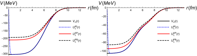
Figure 1: The strong interaction potential between the alpha (⁴He) and the daughter nucleus (²⁰⁶Pb) in the decay of ²¹⁰Po. The left panel shows a comparison of the potentials, $U_{L}^{SP}(r)$ (dot-dashed line), $U_{L}^{PB}(r)$ (dashed line), $U_{L}^{M}(r)$ (dotted line) and the double folding potential $V_{n}(r)$ (solid line) with the knock-on exchange term included. The right panel shows the same without the exchange term. For the sake of this comparison, we choose $\lambda$ = 1 in Eq. (2).

In Fig. 1, we compare the effective potentials with the double folding potential $V_{n}(r)$. To perform this comparison, we choose $\lambda$ = 1 in Eq. (2). Thus, replacing $U_{N}(r)$ with $V_{n}(r)$ of Eq. (2), the Perey-Buck local equivalent potential ($U_{L}^{PB}(r)$) is evaluated using Eq. (19), the São Paulo local equivalent potential ($U_{L}^{SP}(r)$) is evaluated using (20) and the local effective Mumbai potential ($U_{L}^{M}(r)$) using Eq. (24). Since the exchange term in Eq. (3) is often not included in the calculation of the local equivalent potentials neelam1 (in order to avoid double counting of the Pauli nonlocality), we show the potentials with (left panel) as well as without (right panel) this term included. The three potentials, $U_{L}^{PB}(r)$, $U_{L}^{SP}(r)$ and $U_{L}^{M}(r)$ are evaluated for a double folding potential between an alpha and ²⁰⁶Pb nucleus, which are the decay products (and hence originally the cluster nuclei) in the alpha decay of ²¹⁰Po. The nonlocality parameter $\beta$ is taken to be 0.22 fm (explanation given in section VI) , following the prescription given in jackson . The São Paulo and Perey-Buck potentials are quite similar as expected while the energy independent Mumbai potential as mentioned earlier behaves differently at small $r$. The latter, as we shall see in the next section with the example of a simple form for $U_{N}$, follows quite simply from the nonlocal radial equation. The discrepancy between $U_{L}^{PB}$, $U^{SP}_{L}$ and $U^{M}_{L}$ probably arises due to the assumptions in the derivation of Eq. (19).

IV Model dependence at small distances

With the aim of understanding the difference in the small $r$ behaviour of the effective potentials mentioned in the previous section, we shall now analyze the nonlocal kernel using a simple rectangular well for the nuclear potential and try to obtain analytical expressions. Let us begin by considering the integral on the right hand side of Eq. (22), namely, $\displaystyle{\int_{0}^{\infty}\,g_{l}(r,r^{\,\prime})\,u_{l}(r,r^{\,\prime})\,dr^{\,\prime}}$. Given the fact that $g_{l}(r,r^{\,\prime})$ is peaked close to $r=r^{\,\prime}$ (see for example Figs 1a and 5a in Ref. neelam1 ), we perform a Taylor expansion of the wave function about $r=r^{\,\prime}$ and write the above integral as

$$u(r)\,\int_{0}^{\infty}\,g_{l}(r,r^{\,\prime})dr^{\,\prime}\,+\,\int_{0}^{\infty}\,(r^{\,\prime}-r)\,u^{\,\prime}(r)\,g_{l}(r,r^{\,\prime})dr^{\,\prime}\,+\,\cdots$$ (25)

For the case of a rectangular well of depth -$U_{0}$ and range $R$, i.e., for $U_{N}(r)=-U_{0}\Theta(R-r)$ (where $\Theta$ is the Heaviside step function) and assuming $l=0$ for simplicity, we can evaluate the first integral in (25) analytically. Retaining only the first term in the expansion (25) we can define,

$$U_{L}(r)=\int_{0}^{\infty}\,g_{l}(r,r^{\,\prime})dr^{\,\prime}$$ (26)

with,

$$g_{l}(r,r^{\,\prime}) = {2\over\sqrt{\pi}\beta}\,U_{N}\biggl{[}{1\over 2}(r+r^{\prime})\biggr{]}\,\exp{\biggl{[}-{(r^{2}+r^{\prime\,2})\over\beta^{2}}\biggr{]}}\sinh{{2rr^{\prime}\over\beta^{2}}}$$ (27)

$$= -{2\over\sqrt{\pi}\beta}\,U_{0}\,\Theta\biggl{(}R-{r+r^{\prime}\over 2}\biggr{)}\,\exp{\biggl{[}-{(r^{2}+r^{\prime\,2})\over\beta^{2}}\biggr{]}}\,\sinh{{2rr^{\prime}\over\beta^{2}}}\,.$$

One can see that $\Theta$ = 1 only for $2R-r-r^{\prime}>$ 0, i.e., $2R-r>r^{\prime}$ and the upper limit of integration in (26) changes from $\infty$ to $2R-r$. If $r>2R$, $r^{\prime}$ is negative. Hence, to ensure that $r\leq 2R$ we write,

$$U_{L}(r) = {-2U_{0}\over\sqrt{\pi}\beta}\,\Theta(2R-r)\,\int_{0}^{2R-r}\,dr^{\,\prime}\,\exp{\left[-\,{(r^{2}+r^{\,\prime\,2})\over\beta^{2}}\right]}\,\sinh{{2rr^{\,\prime}\over\beta^{2}}}$$

$$= -{U_{0}\over 2}\,\Theta(2R-r)\,\biggl{[}\,erf\biggl{(}{2(R-r)\over\beta}\biggr{)}+2erf\biggl{(}{r\over\beta}\biggr{)}-erf\biggl{(}{2R\over\beta}\biggr{)}\,\biggr{]}.$$

In the limit, $r\to 0$ (for $\beta>0$), since $erf(0)=0$, the potential $U_{L}(r)$ vanishes. When $r$ is finite, we must consider two cases:

$$U_{L}(r) = -{U_{0}\over 2}\,\biggl{[}\,erf\biggl{(}{2(R-r)\over\beta}\biggr{)}+2erf\biggl{(}{r\over\beta}\biggr{)}-erf\biggl{(}{2R\over\beta}\biggr{)}\,\biggr{]}\,\,\,\,\,\,\,\,\,\,\,\,\forall\,\,r<R$$ (29)

$$= -{U_{0}\over 2}\,\biggl{[}\,-erf\biggl{(}{2|R-r|\over\beta}\biggr{)}+2erf\biggl{(}{r\over\beta}\biggr{)}-erf\biggl{(}{2R\over\beta}\biggr{)}\,\biggr{]}\,\,\,\,\,\,\,\,\forall\,\,R<r<2R\,.$$ (30)

If $\beta\to$ 0 (i.e. in the absence of nonlocality), since $erf(\infty)=1$, $U_{L}(r)=-U_{0}$ for $r<R$ and 0 for $R<r<2R$, as expected.

The above derivation on the one hand justifies the behaviour of the Mumbai potential at small $r$ but on the other hand displays an inconsistency between Eqs (IV) and (19). $U_{L}^{PB}(r)$ in Eq. (19), approaches a finite value as $r\to 0$ (for finite $\beta$) as we already noticed in Fig. 1 with a more realistic form of $U_{N}(r)$. However, $U_{L}(r)$, as derived above from the radial nonlocal equation vanishes for $r\to 0$.

Since the starting point for the derivation of the Mumbai potential is indeed the nonlocal radial equation, it seems to be in agreement with the behaviour of $U_{L}(r)$ as in Eq.(IV) but not with that in Eq. (19). The inconsistency between Eq. (19) and Eq. (IV) probably arises due to the approximations made in the derivation of Eq. (19).

V Iterative schemes

Models for the nonlocal nuclear interaction are usually tested for their validity by reproducing scattering data. The solution of the radial equation (22) is obtained by implementing an iterative procedure. The starting point of the iterative procedure involves an effective or local equivalent potential which is a solution of the homogeneous equation such as Eq. (16). For example, the iteration scheme can be started with the local equation,

$${\hbar^{2}\over 2M}\,\biggl{(}{d^{2}\over dr^{2}}-{l(l+1)\over r^{2}}\biggr{)}u^{0}_{l}(r)+(E-U_{L}(r))u^{0}_{l}(r)=0$$ (31)

and followed by

$${\hbar^{2}\over 2M}\,\biggl{(}{d^{2}\over dr^{2}}-{l(l+1)\over r^{2}}\biggr{)}u^{i}_{l}(r)+(E-U_{L}(r))u^{i}_{l}(r)$$ (32)

$$\hskip 28.45274pt=\,\biggl{[}\int_{0}^{R}\,g_{l}(r,r^{\prime})u^{i-1}_{l}(r^{\prime})\,dr^{\prime}\,-\,U_{L}(r)u^{i-1}_{l}(r)\biggr{]}\,,$$

where the suffix $i$ denotes the $i^{th}$ order approximation to the correct solution. The upper limit $R$ is the radius at which the contribution of the kernel becomes negligible. The iteration is continued until the logarithmic derivative at $R$ obtained from $u^{i}_{l}(r)$ agrees up to a certain reasonable precision with the one calculated from $u^{i-1}_{l}(r)$. Generally one finds that a few iterations pereybuck ; neelam1 ; neelam2 already lead to a good agreement with data.

The effect of the nonlocal potentials could in principle be tested by calculating the half lives of radioactive nuclei. Restricting ourselves to the discussion of alpha decay, one could follow a similar iteration scheme as above, however with the difference that $u_{l}(r)$ would have different boundary conditions. Considering the decaying nucleus as a resonant state (and noting that there are no incident particles), the solution of the radial equation would be a “Gamow function” mondragon which vanishes at the origin and behaves as a purely outgoing wave asymptotically. The so-called correct solution obtained from such an iterative scheme could then be used in a quantum mechanical description of the alpha particle decay rates. Such an analysis of the alpha decay of several nuclei could serve as a complementary tool for fixing the parameters or assumptions of the nonlocal models. In order to find out if such a task is worth undertaking, in the present work we take the first step of comparing the alpha decay half lives of some heavy nuclei using different models of the local equivalent (or effective) potentials which satisfy the homogeneous equation. The latter allows us to follow the procedures outlined in Section II to evaluate the half life within the JWKB approximation where the wave function is a solution of the homogeneous equation.

VI Results and Discussions

To study the effect of nonlocality in alpha decay, we evaluate the half-lives of some spherical nuclei (with spin-parity, $J^{P}$ = 0⁺), decaying in the $s$-wave. In order to calculate the half-lives, we use the density dependent double folding model introduced in Section II.1 as input for the evaluation of the effective potentials, $U_{L}$. Note that the nonlocality appears only in the strong part of the potential to which we add the Coulomb and the centrifugal part as given in Section II.1. Since the half-lives are evaluated within the semi-classical JWKB approximation, the potentials are required to satisfy the Bohr-Sommerfeld condition in Eq. (6) which then fixes the strength of $\lambda$ in Eq. (2). In Fig. 2, we compare the full potentials (i.e., Eq. (1) for the double folding potential and $U_{L}(r)\,+\,V_{C}(r)\,+\,{\hbar^{2}\,(l\,+\,1/2)^{2}\over\mu\,r^{2}}$ for the PB, SP and M cases) evaluated for the interaction between ⁴He ($\alpha$) and ²⁰⁶Pb which form the cluster in ²¹⁰Po. In order to evaluate the energy dependent Perey-Buck and São Paulo potentials, we assume the energy to be the $Q$-value (which is approximately the kinetic energy of the alpha in the final state) in the decay of ²¹⁰Po.

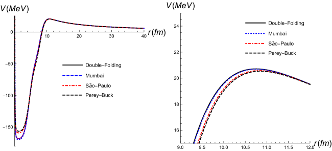
Figure 2: Comparison of the local equivalent potentials for the interaction between ⁴He and ²⁰⁶Pb. The full potentials (including the strong and Coulomb interaction as well as the centrifugal part arising due to the Langer term) are displayed in the left panel. The right panel shows the Coulomb barrier on a different scale. The knock-on exchange term is not included. The values of $\lambda$ appearing in Eq. (2) are listed in Table 3.

Using the three different models for the effective strong interaction, we now evaluate the half-lives in the alpha decay of medium and heavy nuclei. The nonlocality parameter, $\beta$ is given by $\beta=b_{0}m_{0}/\mu$, where $b_{0}$ is the nonlocal range of the nucleon nucleus interaction, $m_{0}$ is the nucleon mass and $\mu$ the alpha-nucleus reduced mass (see jackson for details). We choose $b_{0}$ = 0.85 fm as in Ref. pereybuck , so that $\beta$ = 0.22 fm. The half-lives evaluated with the nonlocality included are found to decrease as compared to those evaluated using the double folding model without nonlocality.

The percentage decrease in half-life due to nonlocality is defined as,

$$PD={\tau_{1/2}^{DF}-\tau_{1/2}^{NL}\over\tau_{1/2}^{DF}}\,\times\,100\,,$$ (33)

where, $\tau_{1/2}^{DF}$ is the half-life evaluated in the double folding model without the inclusion of nonlocalities and $\tau_{1/2}^{NL}$ is the one evaluated using the different nonlocal frameworks. We remind the reader that we choose the cluster preformation factor $P_{\alpha}$ = 1 for this comparison.

In Table 2 we list the percentage decrease in the half-lives of several nuclei. The numbers outside parentheses correspond to calculations with the so called knock-on exchange term excluded in order to avoid double counting of the Pauli nonlocality. Inclusion of this term (numbers in parentheses) causes a larger percentage decrease of half-lives due to nonlocality within the Perey-Buck and São Paulo models. The effect of nonlocality is in general small within the Mumbai approach. Apart from this, we note that the effect of nonlocality is smaller in the decay of ²¹²Po (Q = 8.954 MeV) as compared to ²¹⁰Po (5.407 MeV). Though the difference is not large, it hints towards a decrease in the effect of nonlocality with increasing energy in the two isotopes.

Table 2: Percentage decrease, $PD$ as in Eq. (33), in alpha decay half-lives of nuclei using three different models of nonlocality. Numbers within parentheses include the effect of the so called knock-on exchange term and those outside ignore this term. The nonlocality parameter $\beta$ = 0.22 fm.

	Mumbai	São Paulo	Perey-Buck
254Fm	2.49 (3.85)	31.7 (69.8)	40.3 (71.5)
210Po	3.4 (2.4)	29.9 (66.2)	37.3 (67.9)
212Po	3.26 (3.28)	26.7(62.0)	33.0 (63.8)
180W	3.8 (4.0)	30.1 (66.1)	37.6 (67.7)
168Pt	4.9 (4.1)	27.5 (62.7)	34.9 (64.9)
144Nd	3.9 (3.8)	25.9 (60.3)	31.2 (61.9)
106Te	3.2 (4.1)	19.4 (51.9)	24.1 (53.6)

In order to understand the results in Table 2, let us examine Fig. 2 and the factors presented in Table 3. We consider the numbers outside the parentheses in Table 2 which means that the knock-on exchange term is not included in the calculation of $V_{n}$. The full potentials given in Fig. 2 are obtained using Eqs (1) and (2) with the values of $\lambda$ (listed in Table 3) being fixed by the Bohr-Sommerfeld condition (6). Assuming $P_{\alpha}$ = 1 and rewriting the expression for the width in (8) as

$$\Gamma={\hbar^{2}\over 2\,\mu}\ NP\,,$$

where, the normalization factor $N=[\,\int_{r_{1}}^{r_{2}}\,{dr/k(r)}\,]^{-1}$ and the exponential factor or the penetration probability, $P=e^{-2\int_{r_{2}}^{r_{3}}\,k(r)\,dr}$, we note from Table 3 that it is indeed the difference in the penentration probabilities, $P$, which leads to the differences in the percentage decrease in the half-lives in Table 2. The normalization factors are almost constant in all models. This fact is also reflected in Fig. 2. In the right panel we notice that the Coulomb potential in the São Paulo and Perey-Buck models is shifted to the right as compared to the double-folding and Mumbai potentials. This shift leads to a shift of the second turning point, $r_{2}$, to bigger values and hence smaller half-lives (due to the bigger exponential factor as can be seen in Table 3).

Table 3: Factors contributing to the calculated half-lives in different models. The strength of the strong interaction, $\lambda$, which is fixed by the Bohr-Sommerfeld condition (6), the normalization factor N = $[\int_{r_{1}}^{r_{2}}dr/k(r)]^{-1}$ and the penetration probability, P$=e^{-2\int_{r_{2}}^{r_{3}}\,k(r)\,dr}$, are listed in all models for each of the nuclei considered. The knock-on exchange term is not included.

Isotope	Q-Value	Double Folding			Mumbai			São Paulo			Perey Buck
		$\lambda$	P	N	$\lambda$	P	N	$\lambda$	P	N	$\lambda$	P	N
	[MeV]			[fm-2]			[fm-2]			[fm-2]			[fm-2]
254Fm	7.307	1.95	$3\times 10^{-25}$	0.34	1.96	$3.1\times 10^{-25}$	0.34	2.08	$4.5\times 10^{-25}$	0.34	2.30	$5.2\times 10^{-25}$	0.34
212Po	8.954	2.02	$3\times 10^{-14}$	0.34	2.03	$3.2\times 10^{-14}$	0.34	2.17	$4.2\times 10^{-14}$	0.33	2.36	$4.6\times 10^{-14}$	0.33
210Po	5.407	2.10	$5.4\times 10^{-27}$	0.36	2.12	$5.6\times 10^{-27}$	0.35	2.25	$7.8\times 10^{-27}$	0.35	2.45	$8.6\times 10^{-27}$	0.36
180W	2.515	2.04	$2\times 10^{-46}$	0.36	2.05	$2.1\times 10^{-46}$	0.36	2.17	$2.8\times 10^{-46}$	0.36	2.35	$3.1\times 10^{-46}$	0.35
168Pt	6.989	2.08	$3\times 10^{-18}$	0.35	2.10	$3.2\times 10^{-18}$	0.35	2.22	$4.2\times 10^{-18}$	0.35	2.41	$4.6\times 10^{-18}$	0.35
144Nd	1.903	2.23	$3.6\times 10^{-44}$	0.37	2.26	$3.8\times 10^{-44}$	0.37	2.39	$4.9\times 10^{-44}$	0.36	2.55	$5.3\times 10^{-44}$	0.36
106Te	4.290	2.28	$6.2\times 10^{-17}$	0.35	2.30	$6.5\times 10^{-17}$	0.35	2.43	$7.9\times 10^{-17}$	0.35	2.58	$8.4\times 10^{-17}$	0.35

Before closing the discussions, some comments about one of the earliest investigations of nonlocalities in alpha decay are in order here. In a series of works chaudhury1 ; chaudhury2 ; chaudhury3 ; chaudhury4 , M. L. Chaudhury studied the effects of nonlocalities in alpha decay of different nuclei. Using an integro-differential equation similar to that of Frahn and Lemmer frahnlemmer , in Ref. chaudhury1 , the author calculated the transmission coefficient (or penetration factor) for alpha tunneling within the WKB approximation. The point-like Coulomb field was superimposed by a nonlocal alpha-nucleus interaction based on the Igo potential igo and a Gaussian form was used for the nonlocal function with a nonlocality parameter of $\beta$ = 0.9 fm. Investigating for the alpha decay of ²⁵⁴Fm in Ref. chaudhury1 , the penetration factor was found to increase by a factor of 1.7 due to nonlocality. This amounts to a decrease of about 40 % in the half-life. The investigation in Ref. chaudhury1 was extended to several even-even nuclei and the author once again found a large increase ($\sim$ 50 %) chaudhury2 in the penetration factors due to nonlocality. The author further studied the effects of nonlocality in deformed and rare earth nuclei chaudhury3 ; chaudhury4 with the inclusion of an exchange term in the nonlocal kernel. Though the calculation in Ref. chaudhury1 involves a different nonlocal framework as compared to the models considered in the present work, the 40% decrease in the value of the half-life of ²⁵⁴Fm chaudhury1 (evaluated without the exchange term in the nonlocal kernel), is similar to the Perey-Buck model result in Table 2, without the inclusion of the knock-on exchange term.

VII Summary

Investigation of the effects of nonlocality in the nuclear interaction began several decades ago but has remained to be a topic of continued interest until now. The vast majority of works proposing different approaches to understand the origin as well as the manifestations of the nonlocality concentrate on the reproduction of scattering data. Here, we have proposed the study of the effects of nonlocality on alpha decay half lives of nuclei as a complementary tool for determining the nonlocal interaction within different models.

To be specific, we have studied these effects using three different models available in literature. Though all the three models agree qualitatively on the result that the nonlocal nuclear interaction leads to a decrease in half-lives, the percentage decrease in the three models is quite different. The recent Mumbai model neelam1 ; neelam2 predicts a very small percentage decrease of about 2 - 5% in most heavy nuclei studied, however, the Perey-Buck and São Paulo models predict a much bigger decrease of around 20 - 40% (in the absence of the knock-on exchange term).

In order to understand the above differences, we examined the model assumptions in detail and found an inconsistency in the behaviour of the local equivalent potentials, $U_{L}(r)$, derived by starting with the 3-dimensional Schrödinger equation and the radial one. Whereas the former leads to $U_{L}(r)$ which is finite at the origin, the latter vanishes for $r\to 0$. Indeed the Perey-Buck and the São Paulo models are of the former type (with the local equivalent potential being finite at $r$ = 0) but the effective potential of the Mumbai group vanishes at $r$ = 0. Introducing the nonlocal framework to find the Gamow functions corresponding to the decaying nuclei and performing a more exact quantum mechanical calculation of the half lives to compare with data could possibly provide a better explanation of the different behaviours of the potentials.

- (1) S. Q. Hou et al., Astrophys. J 834, 165 (2017).
- (2) N. G. Kelkar and D. Bedoya Fierro, Phys. Lett. B 772, 159 (2017).
- (3) H. Bethe Phys. Rev. 103, 1353 (1956).
- (4) W. E. Frahn, Nuovo Cimento 4, 313 (1956).
- (5) R. Peierls and N. Vinh Mau, Nucl. Phys. A 343, 1 (1980).
- (6) F. Perey and B. Buck, Nucl. Phys. 32, 353 (1962).
- (7) A. B. Balantekin, J. F. Beacom and M. A. Cndido Ribeiro, J. Phys. G 24, 2087 (1998).
- (8) L. C. Chamon et al., Brazilian J. Phys. 33, 238 (2003).
- (9) N. J. Upadhyay, A. Bhagwat and B. K. Jain, J. Phys. G 45, 015106 (2018).
- (10) N. J. Upadhyay and A. Bhagwat, Phys. Rev. C 98, 024605 (2018).
- (11) N. G. Kelkar and H. M. Castañeda, Phys. Rev. C 76, 064605 (2007).
- (12) N. G. Kelkar, H. M. Castañeda and M. Nowakowski, Eur. Phys. Lett. 85, 20006 (2009).
- (13) N. G. Kelkar and M. Nowakowski, J. Phys. G 43, 105102 (2016).
- (14) D. Ni and Z. Ren, Annals of Phys. 358, 108 (2015).
- (15) C. Xu and Z. Ren, Nucl. Phys. A 760, 303 (2005); ibid, Phys. Rev. C 74, 014304 (2006); ibid, Nucl. Phys. A 753, 174 (2005); ibid, Phys. Rev. C 73, 041301(R) (2006).
- (16) N. K. Glendenning, Direct Nuclear Reactions (Academic Press, New York, 1983), p. 42.
- (17) R. E. Langer, Phys. Rev. 51, 669 (1937).
- (18) N. Fröman, JWKB Approximation: Contributions to the Theory (North-Holland Pub. Co., Amsterdam, 1965); N. Fröman and Per Olof Fröman, Physical Problems Solved by the Phase-Integral Method (Cambridge University Press, 2002).
- (19) J. J. Morehead, J. Math. Phys. 36, 5431 (1995).
- (20) G. R. Satchler and W. G. Love, Phys. Rep. 55, 183 (1979); A. M. Kobos, G. R. Satchler and A. Budzanowski, Nucl. Phys. A 384, 65 (1982).
- (21) J. D. Walecka, Theoretical Nuclear Physics and Subnuclear Physics (Oxford University, Oxford, 1995), p. 11; B. Hahn, D. G. Ravenhall, and R. Hofstadter, Phys. Rev. 101, 1131 (1956).
- (22) B. Buck, A. C. Merchant and S. M. Perez, Phys. Rev. C 45, 2247 (1992); B. Buck, J. C. Johnston, A. C. Merchant and S. M. Perez, Phys. Rev. C 53, 2841 (1996).
- (23) J. K. Tuli, Nuclear Wallet Cards, NNDC, Brookhaven National Laboratories (2011) (can be downloaded at www.nndc.bnl.gov/wallet).
- (24) C. Xu et al., Phys. Rev. C 93, 011306(R) (2016).
- (25) C. Xu et al., Phys. Rev. C 95, 061306(R) (2017).
- (26) L. Chamon et al., Phys. Rev. Lett. 79, 5218 (1997).
- (27) L. C. Chamon, B. V. Carlson and L. R. Gasques, Phys. Rev. 83, 034617 (2011).
- (28) L. C. Chamon, L. R. Gasques and B. V. Carlson, Phys. Rev. C 84, 044607 (2011).
- (29) A. Mondragon and E. Hernandez, Ann. Physik Leipzig 48, 503 (1991).
- (30) D. F. Jackson and R. C. Johnson, Phys. Lett. 49 B, 249 (1974).
- (31) M. L. Chaudhury, Phys. Rev. Lett. 5, 205 (1960).
- (32) M. L. Chaudhury, Phys. Rev. 130, 2339 (1963).
- (33) M. L. Chaudhury, J. Phys. A 4, 328 (1971).
- (34) M. L. Chaudhury and D. K. Sen, J. Physique 42, 19 (1981).
- (35) W. E. Frahn and R. H. Lemmer, Nuova Cimento 5, 1567 (1957).
- (36) I. Igo and R. M. Thaler, Phys. Rev. 106, 126 (1957).