What does kinematical target mass sensitivity in DIS
reveal about hadron structure?

Abstract

We study the role of purely external kinematical approximations in inclusive deep-inelastic lepton–hadron scattering within QCD factorization, and consider factorization with an exact treatment of the target hadron mass. We discuss how an observed phenomenological improvement obtained by accounting for target mass kinematics could be interpreted in terms of general properties of target structure, and argue that such an improvement implies a hierarchy of nonperturbative scales within the hadron.

I Introduction

Understanding the nature of confined systems of strongly interacting quarks and gluons (or partons), such as hadrons and nuclei, remains one of the single most challenging problems in nuclear and particle physics. An essential tool in this quest has been the factorization of the short- and long-distance parts of scattering amplitudes, which has allowed the systematic study of hard scattering processes in terms of universal sets of parton distribution functions (PDFs) Collins et al. (1988). While this has proved an enormously successful paradigm when applied to reactions at high energies, where typical momentum transfers $Q$ are much greater than any hadronic mass scales, $Q\gg O(1~{}{\rm GeV})$, delineating the extent to which factorization techniques may be applicable at lower energies has been a rather more formidable task.

The transition region at intermediate momentum transfers, $Q\sim 1$ – 2 GeV, where descriptions of phenomena in terms of parton degrees of freedom give way to nonperturbative dynamics, is still poorly understood. Here small-coupling quantum chromodynamics (QCD) techniques are often applicable, while at the same time hadronic mass effects are not always negligible. Phenomena specific to the this regime, such as quark-hadron duality Bloom and Gilman (1971); De Rújula et al. (1977a); Poggio et al. (1976); Ji and Unrau (1995); Melnitchouk et al. (2005) and precocious scaling Duke and Roberts (1980); Devoto et al. (1983) have attracted much interest, and it has been the focus of dedicated experimental efforts at Jefferson Lab Christy and Melnitchouk (2011); Chen et al. (2011); Gilman et al. (2011).

Extending standard perturbative QCD (and even general partonic pictures) to the low-$Q$ region also presents theoretical challenges, particularly since certain mass effects that are normally treated as negligible in QCD processes with large $Q$ may become important there. Consider the basic statement of factorization for the inclusive lepton–nucleon (or any other hadron or nucleus) DIS cross section (see, e.g., Ref. Collins et al. (1988)),

$$\frac{\mathrm{d}\sigma}{\mathrm{d}x_{\rm Bj}{}\mathrm{d}Q^{2}{}}=\int\!\mathrm{d}\xi\,\frac{\mathrm{d}\hat{\sigma}}{\mathrm{d}\hat{x}_{\rm Bj}{}\mathrm{d}Q^{2}{}}\,f(\xi;Q)+{\rm p.s.}\,,$$ (1)

where $x_{\rm Bj}=Q^{2}/2P\cdot q$ is the Bjorken scaling variable, with $P$ and $q$ the target nucleon and exchanged virtual photon momenta, respectively, and for simplicity we omit explicit flavor dependence. The partonic differential cross section $\mathrm{d}\hat{\sigma}$ is expressed in terms of the corresponding scaling variable $\hat{x}_{\rm Bj}=Q^{2}/2\,\hat{k}\cdot q$ for the target parton with momentum $\hat{k}$ in the subprocess (see Fig. 1 below). The function $f(\xi;Q)$ is to be interpreted as a probability distribution of partons with fraction $\xi=\hat{k}^{+}/P^{+}$ of the nucleon’s light-cone momentum, with extra scale dependence induced by QCD evolution. The first term in Eq. (1) is the end result of a sequence of canonical approximations which increase in accuracy as $Q$ increases with fixed $x_{\rm Bj}$ Collins (2011), while the second term represents power suppressed (“${\rm p.s.}$”) errors that are proportional to powers of $1/Q^{2}$ relative to the first term. Factorization then describes the limit of large $Q$, with $x_{\rm Bj}$ fixed, where these error terms can safely be ignored.

Knowing the exact value of the correction term in Eq. (1) requires a much deeper understanding of complex QCD dynamics than what is treated by the usual factorization. However, there are certain standard approximations (see, e.g., Ref. (Ellis et al., 1996, p. 95)) contributing to the error in Eq. (1) that deal only with the external kinematics of $P$ and $q$ and have nothing specifically to do with the dynamics of the deeply inelastic collision. These are what we will mean by “purely kinematical” approximations. The most common of these is a target mass approximation in inclusive DIS: if the target is moving in light-cone variables with large “$+$” momentum and zero transverse momentum, then $P^{\mu}=(P^{+},M^{2}/2P^{+},\boldsymbol{0}_{\text{T}}{})\approx(P^{+},0,\boldsymbol{0}_{\text{T}}{})$. As will be discussed in detail below, the resulting errors are proportional to powers of $x_{\rm Bj}^{2}M^{2}/Q^{2}$, where $M$ is the target nucleon mass.

By contrast, the derivation of factorization uses approximations on internal partonic constituents, whose exact properties depend on complex details of QCD dynamics. The resulting error terms are suppressed by powers of $m^{2}/Q^{2}$, where $m$ here represents any of the scales associated with intrinsic dynamical properties of bound state partons, such as their virtualities. Since the factorization theorem is meant to describe the limiting behavior as $1/Q^{2}\to 0$, the $x_{\rm Bj}^{2}M^{2}/Q^{2}$ errors from the kinematical expansion are typically lumped with the dynamical $m^{2}/Q^{2}$ errors. We will, however, refrain from identifying the $O\left(x_{\rm Bj}^{2}M^{2}/Q^{2}\right)$ terms as a contribution to the $O\left(m^{2}/Q^{2}\right)$ corrections in all our discussions so as to emphasize the different origins of these two types of errors.

Of course, all mass scales are ultimately fixed by the QCD scale parameter $\Lambda_{\rm QCD}^{2}$, so the internal scales we associate with $m^{2}$ should be understood to be proportional to $M^{2}$: $m^{2}=\eta M^{2}$, with $\eta$ being a dimensionless proportionality factor. So another way then to state the above is that we will consider expansions in powers of $\eta M^{2}/Q^{2}$ separately from powers of $M^{2}/Q^{2}$. This is explained in more detail in Secs. III and IV.

At moderate $Q$, a natural question is whether all of the various types of contributions to the error term in Eq. (1) are really so negligible and, if not, whether some improvement is possible. For instance, when $Q\sim 1$ GeV and $x_{\rm Bj}$ is not especially small ($x_{\rm Bj}\sim 1$), the $x_{\rm Bj}^{2}M^{2}/Q^{2}$ purely kinematical errors may no longer be negligible. Since they arise only from kinematical approximations, it is reasonable to ask if these purely kinematical errors can be removed with minimal or no modification to the basic correctness of the factorization derivation for the first term in Eq. (1). In fact, as we will discuss in Sec. IV, the standard derivations do not actually require a massless target approximation. Setting the target mass to zero is an ancillary step, while keeping it nonzero leads naturally to Nachtmann scaling Nachtmann (1973). This was actually recognized some time ago by Aivazis, Olness and Tung (AOT) Aivazis et al. (1994) in the context of heavy quark contributions in DIS.

Questions of interpretation remain, however. It must be established, for example, whether it is reasonable to expect that correction for kinematical mass errors will result in phenomenological improvements in applications of QCD factorization. That it should is not obvious since there is no reason a priori to assume one type of power correction is more important than another. The mass scales divided by $Q^{2}$ that contribute errors to factorization originate from nonperturbative features of the target hadron, so the effectiveness of target mass improvements must be tied to specific features of individual targets. Questions concerning the relevance of target mass kinematics therefore cannot generally be disentangled from questions about hadron structure.

In this paper we will argue that it is most natural to expect an improvement from the approach of AOT Aivazis et al. (1994) if the structure of the target involves a hierarchy of nonperturbative scales. Keeping certain powers of $1/Q^{2}$ while neglecting others makes sense only when there is a reasonably large variation in mass-squared factors in the numerators. Questions about the phenomenological usefulness of kinematical target mass corrections can then be reframed as questions about target structure. This is how we advocate addressing the issue of target mass kinematics more generally, as explained in more detail in Sec. V. Before this, in Sec. II we introduce the basic kinematics of the DIS process at finite energy, keeping all masses in the structure functions and the kinematic variables on which they depend. In Sec. III we introduce the massless target approximation, carefully defining projection operators and structure functions in the limit of small $M^{2}/Q^{2}$. The factorization of the DIS process into a hard scattering subprocess from massless and on-shell partons is outlined in Sec. IV, where we write down the explicit formulas for the structure functions in terms of partonic scattering amplitudes and nonperturbative PDFs. The relation between TMC improvement and nonperturbative scale hierarchy is discussed in Sec. V. Finally, in Sec. VI we summarize our results and suggest extensions of our analysis to other applications.

II Deep-inelastic scattering kinematics

The reaction we will consider in the present work is inclusive lepton scattering from a target hadron, such as a nucleon, $l(l)+N(P)\to l^{\prime}(l^{\prime})+X(P_{X})$, where $l^{\mu}$ and $l^{\prime\mu}$ are the incident and scattered lepton four-momenta, and $P^{\mu}$ and $P_{X}^{\mu}$ are the four-momenta of the target nucleon and hadronic final state $X$, respectively. The reaction will be assumed to proceed through the exchange of a virtual photon with four-momentum $q^{\mu}=l^{\mu}-l^{\prime\mu}$. To make the calculation more transparent, we work in a frame where the nucleon moves in the $+z$ direction, the exchanged virtual photon moves in the $-z$ direction, and both have zero transverse momentum. In this case the nucleon and photon four-momenta are conveniently parametrized in terms of light-front coordinates as

$$P^{\mu}=\left(P^{+},\,\frac{M^{2}}{2P^{+}},\,\boldsymbol{0}_{\text{T}}{}\right)\,,\qquad q^{\mu}=\left(-x_{\rm N}P^{+},\,\frac{Q^{2}}{2x_{\rm N}P^{+}},\,\boldsymbol{0}_{\text{T}}{}\right)\,,$$ (2)

where $Q\equiv\sqrt{-q^{2}}$, and $x_{\rm N}$ is the Nachtmann scaling variable Greenberg and Bhaumik (1971); Nachtmann (1973),

$$x_{\rm N} \equiv-\frac{q^{+}}{P^{+}}=\frac{2x_{\rm Bj}}{1+\sqrt{1+4x_{\rm Bj}^{2}M^{2}/Q^{2}}},$$ (3)

so that the Bjorken variable can also be written

$$x_{\rm Bj} = \frac{Q^{2}}{2P\cdot q}\ =\ \frac{x_{\rm N}}{(1-x_{\rm N}^{2}M^{2}/Q^{2})}\,.$$ (4)

In the Breit frame, where the photon has zero energy, the target has $P^{+}=Q/(\sqrt{2}x_{\rm N})$ and the four-momenta simplify to

$$P^{\mu}=\left(\frac{Q}{\sqrt{2}x_{\rm N}},\,\frac{x_{\rm N}M^{2}}{\sqrt{2}Q},\,\boldsymbol{0}_{\text{T}}{}\right)\,,\qquad q^{\mu}=\left(-\frac{Q}{\sqrt{2}},\,\frac{Q}{\sqrt{2}},\,\boldsymbol{0}_{\text{T}}{}\right).$$ (5)

The total inclusive cross section is expressed as a contraction of leptonic and hadronic tensors,

$$E^{\prime}\frac{\mathrm{d}\sigma{}}{\mathrm{d}^{3}\boldsymbol{l}^{\prime}{}}=\frac{2\alpha_{\rm em}^{2}}{\left(s-M^{2}\right)Q^{4}}\;L_{\mu\nu}W^{\mu\nu},$$ (6)

where $E^{\prime}$ is the energy of the scattering lepton, $s=(l+P)^{2}$ is the invariant mass squared of the system, and $\alpha_{\rm em}=e^{2}/4\pi$ is the electromagnetic fine structure constant. The leptonic tensor is

$$L_{\mu\nu}=2(l_{\mu}l^{\prime}_{\nu}+l^{\prime}_{\mu}l_{\nu}-g_{\mu\nu}l\cdot l^{\prime}),$$ (7)

and the totally inclusive hadronic tensor is defined as

$$W^{\mu\nu}(P,q) {}\equiv 4\pi^{3}\sum_{X}\delta^{(4)}(P+q-P_{X})\,\langle P|j^{\mu}(0)|X\rangle\langle X|j^{\nu}(0)|P\rangle.$$ (8)

Here, the $\sum_{X}$ symbol represents a sum over all possible final states $|X\rangle$, including integrals

$$\int\!\frac{\mathrm{d}^{3}\boldsymbol{P}_{X}{}}{(2\pi)^{3}2E_{P_{X}}}\,.$$

For spin-averaged, parity-conserving scattering the hadronic tensor can then be expanded into dimensionless structure functions according to

$$W^{\mu\nu} =\left(-g^{\mu\nu}+\frac{q^{\mu}q^{\nu}}{q^{2}}\right)F_{1}\left(x_{\rm Bj}(x_{\rm N},M^{2}/Q^{2}),Q^{2}\right)$$

$${}+\left(P^{\mu}-\frac{P\cdot q}{q^{2}}q^{\mu}\right)\left(P^{\nu}-\frac{P\cdot q}{q^{2}}q^{\nu}\right)\frac{F_{2}\big{(}x_{\rm Bj}(x_{\rm N},M^{2}/Q^{2}),Q^{2}\big{)}}{P\cdot q}\,.$$ (9)

The structure functions take all Lorentz invariants formed by $P$ and $q$ as arguments. These include $P\cdot q$ and $Q^{2}$, while independent mass dependence is left implicit. Instead of $P\cdot q$ we choose $x_{\rm Bj}$ as the independent variable, although it turns out that $x_{\rm N}$, in fact, is a more natural choice in the context of factorization. We will continue to use the Bjorken variable $x_{\rm Bj}$, however, since that is the more traditional choice, but will write it in the form $x_{\rm Bj}(x_{\rm N},M^{2}/Q^{2})$, as a function of $x_{\rm N}$ and $M^{2}/Q^{2}$ explicitly. While this may appear cumbersome initially, it will help make later approximation steps unambiguous.

The structure functions $F_{i}$ ($i=1,2$) can be calculated from the hadronic tensor $W_{\mu\nu}$ using projection tensors,

$$F_{i}\left(x_{\rm Bj}(x_{\rm N},M^{2}/Q^{2}),Q^{2}\right)={\rm P}_{i}^{\mu\nu}\left(x_{\rm N},Q,M\right)\,W_{\mu\nu}(P,q)\,,\qquad[i=1,2]$$ (10)

defined by

$${\rm P}_{1}^{\mu\nu}{} \equiv-\frac{1}{2}g^{\mu\nu}+\frac{2Q^{2}x_{\rm N}^{2}}{(Q^{2}+M^{2}x_{\rm N}^{2})^{2}}P^{\mu}P^{\nu}\ ,$$ (11a)

$${\rm P}_{2}^{\mu\nu}{} \equiv\frac{12Q^{4}x_{\rm N}^{3}\left(Q^{2}-M^{2}x_{\rm N}^{2}\right)}{\left(Q^{2}+M^{2}x_{\rm N}^{2}\right)^{4}}\bigg{(}P^{\mu}P^{\nu}-\frac{\left(Q^{2}+M^{2}x_{\rm N}^{2}\right)^{2}}{12Q^{2}x_{\rm N}^{2}}g^{\mu\nu}\bigg{)}\,.$$ (11b)

Up to this point all of the expressions for the cross sections and structure functions are for exact kinematics. In the next section we consider the limit in which the mass of the target is taken to be much smaller than the scale $Q$, $M/Q\ll 1$.

III Massless Target Approximation (MTA)

Purely kinematical approximations are those which can be defined in the context of Sec. II; that is, by considering only overall external momentum and with no reference to hadrons’ constituents or other dynamical properties. A kinematical approximation replaces $P$ and $q$, and the arguments of the structure functions $F_{i}\big{(}x_{\rm Bj}(x_{\rm N},M^{2}/Q^{2}),Q^{2}\big{)}$, by different, approximated quantities, without changing anything about the functions in Eq. (9) themselves.

Let us define the natural approximate target hadron four-momentum $\widetilde{P}$ in a frame where it is moving at relativistic speeds by setting the target mass to zero,

$$P\to\widetilde{P}\equiv(P^{+},0,\boldsymbol{0}_{\text{T}}{})\,.$$ (12)

The massless target approximation (MTA) is the kinematical approximation defined by the replacement

$$P\cdot q\ \to\ \widetilde{P}\cdot q\,,$$

wherever this occurs in Eq. (8). To set up the approximation, it is convenient to first switch the structure function decomposition to a basis that uses $\widetilde{P}$ instead of $P$,

$$W^{\mu\nu} =\left(-g^{\mu\nu}+\frac{q^{\mu}q^{\nu}}{q^{2}}\right)\widetilde{F}_{1}\left(x_{\rm Bj}(x_{\rm N},M^{2}/Q^{2}),Q^{2}\right)$$

$${}+\left(\widetilde{P}^{\mu}-\frac{\widetilde{P}\cdot q}{q^{2}}q^{\mu}\right)\left(\widetilde{P}^{\nu}-\frac{\widetilde{P}\cdot q}{q^{2}}q^{\nu}\right)\frac{\widetilde{F}_{2}\big{(}x_{\rm Bj}(x_{\rm N},M^{2}/Q^{2}),Q^{2}\big{)}}{\widetilde{P}\cdot q}\,.$$ (13)

Here we have defined

$$\widetilde{F}_{i}\left(x_{\rm Bj}(x_{\rm N},M^{2}/Q^{2}),Q^{2}\right)\ \equiv\ \widetilde{\rm P}_{i}^{\mu\nu}\ W_{\mu\nu}\,,\hskip 42.67912pt[i=1,2]$$ (14)

with the corresponding tensors to project out the structure functions defined by

$$\widetilde{\rm P}_{1}^{\mu\nu} \equiv{\rm P}_{1}^{\mu\nu}\big{(}x_{\rm N},Q,0\big{)}=-\frac{1}{2}\bigg{(}g^{\mu\nu}-\frac{4x_{\rm N}^{2}}{Q^{2}}\widetilde{P}^{\mu}\widetilde{P}^{\nu}\bigg{)}\,,$$ (15a)

$$\widetilde{\rm P}_{2}^{\mu\nu} \equiv{\rm P}_{2}^{\mu\nu}\big{(}x_{\rm N},Q,0\big{)}=-x_{\rm N}\bigg{(}g^{\mu\nu}-\frac{12x_{\rm N}^{2}}{Q^{2}}\widetilde{P}^{\mu}\widetilde{P}^{\nu}\bigg{)}\,.$$ (15b)

This is a more convenient basis if we ultimately want to neglect the minus component of $P$. Note that it is $x_{\rm N}$ that appears in the factors on the right side of Eqs. (15), and not $x_{\rm Bj}$. To relate structure functions in the two bases, we use

$$\left(\widetilde{\rm P}_{i}^{\mu\nu}\ W_{\mu\nu}\right)_{\text{Eq.~{}(\ref{e.Wmunu})}}=\left(\widetilde{\rm P}_{i}^{\mu\nu}\ W_{\mu\nu}\right)_{\text{Eq.~{}(\ref{e.Wmunutilde})}}\,.$$ (16)

Applying the projectors (15) gives

$$\widetilde{F}_{1}\left(x_{\rm Bj}(x_{\rm N},M^{2}/Q^{2}),Q^{2}\right) {}=F_{1}\left(x_{\rm Bj}(x_{\rm N},M^{2}/Q^{2}),Q^{2}\right),\,$$ (17a)

$$\widetilde{F}_{2}\left(x_{\rm Bj}(x_{\rm N},M^{2}/Q^{2}),Q^{2}\right) {}=\frac{\left(Q^{2}+M^{2}x_{\rm N}^{2}\right)^{2}}{Q^{2}\left(Q^{2}-M^{2}x_{\rm N}^{2}\right)}\,F_{2}\left(x_{\rm Bj}(x_{\rm N},M^{2}/Q^{2}),Q^{2}\right)\,.$$ (17b)

We stress that no approximation has been made in the discussion up to this point. The coefficients in front of the structure functions in Eqs. (17) are, in fact, the same as those in the literature that are referred to as “$\xi$-scaling” Aivazis et al. (1994); Kretzer and Reno (2002); Schienbein et al. (2008); Accardi and Qiu (2008); Brady et al. (2011). The first step in the MTA is the replacement of $x_{\rm Bj}(x_{\rm N},M^{2}/Q^{2})$ by $x_{\rm Bj}(x_{\rm N},0)$ in the structure functions in Eq. (13),

$$W^{\mu\nu}\ \stackrel{{\scriptstyle\rm MTA}}{{\longrightarrow}}\ \widetilde{W}^{\mu\nu} = \bigg{(}-g^{\mu\nu}+\frac{q^{\mu}q^{\nu}}{q^{2}}\bigg{)}\widetilde{F}_{1}\left(x_{\rm Bj}(x_{\rm N},0),Q^{2}\right)\,$$ (18)

$$+ \bigg{(}\widetilde{P}^{\mu}-\frac{\widetilde{P}\cdot q}{q^{2}}q^{\mu}\bigg{)}\bigg{(}\widetilde{P}^{\nu}-\frac{\widetilde{P}\cdot q}{q^{2}}q^{\nu}\bigg{)}\frac{\widetilde{F}_{2}\left(x_{\rm Bj}(x_{\rm N},0),Q^{2}\right)}{\widetilde{P}\cdot q}\,,$$

where $\widetilde{W}^{\mu\nu}$ is the approximate hadronic tensor. In this approximation, Eq. (4) gives

$$x_{\rm Bj}(x_{\rm N},0)=x_{\rm N}\,,$$ (19)

so that $x_{\rm Bj}$ and $x_{\rm N}$ are interchangeable in the MTA.

The above discussion suggests a definition for the target mass approximated structure functions $\mathcal{F}_{i}$,

$$\mathcal{F}_{i}\left(x_{\rm Bj},Q^{2}\right)\equiv\widetilde{F}_{i}\left(x_{\rm Bj}(x_{\rm N},0),Q^{2}\right)\,,$$ (20)

where the script notation is a shorthand that means $x_{\rm Bj}(x_{\rm N},M^{2}/Q^{2})$ is understood to be everywhere replaced by $x_{\rm Bj}(x_{\rm N},0)$, so that kinematical dependence on the ratio $M^{2}/Q^{2}$ is neglected. Part of the MTA is to approximate structure functions defined in the “tilde” [Eq. (13)] and “non-tilde” [Eq. (9)] bases as being the same. From Eqs. (17), this also introduces only an $O\left(M^{2}/Q^{2}\right)$ error. Expanding the structure functions in powers of $M^{2}/Q^{2}$ gives a concise expression of the MTA,

$$F_{i}\left(x_{\rm Bj}(x_{\rm N},M^{2}/Q^{2}),Q^{2}\right) {}=\widetilde{F}_{i}\left(x_{\rm Bj}(x_{\rm N},M^{2}/Q^{2}),Q^{2}\right)+O\left(\frac{x_{\rm Bj}^{2}M^{2}}{Q^{2}}\right)$$

$${}=\widetilde{F}_{i}\left(x_{\rm Bj}(x_{\rm N},0),Q^{2}\right)+O\left(\frac{x_{\rm Bj}^{2}M^{2}}{Q^{2}}\right)$$

$${}=\mathcal{F}_{i}\left(x_{\rm Bj},Q^{2}\right)+O\left(\frac{x_{\rm Bj}^{2}M^{2}}{Q^{2}}\right)\,,$$ (21)

where the approximation is to drop all the $x_{\rm Bj}^{2}M^{2}/Q^{2}$ errors. In other words, assuming an exact hadronic tensor in Eq. (8), the MTA [Eqs. (14)–(18)] is equivalent to a set of natural argument replacements that are reasonable when $Q$ is very large or $x_{\rm Bj}$ is very small. This approximation is usually made implicitly in discussions of high energy scattering in the literature Ellis et al. (1996); here we have made it very explicit so that it will be straightforward to reverse it. Each step in Eq. (21) can be traced back to the unapproximated hadronic tensor and structure functions. Operationally, it is implemented by the replacement in Eq. (18).

This completes our general discussion of the exact and target mass approximated structure functions, based on considerations of external kinematics alone. In the remainder of the paper we will specialize the discussion to the role of the target mass in collinear factorization.

IV The MTA and Collinear Factorization

In this section we discuss how the MTA of the last section, combined with the standard factorization steps Collins (2011), leads to the well-known collinear factorization theorem of Eq. (1). Again, we will present the steps in greater detail than is common in the literature, which will help later to unravel the source of purely kinematical mass sensitivity.

Before any factorization approximations are made, the exact parton momentum $k$ can in general have both a virtuality and transverse momentum,

$$k=\left(\xi P^{+},\frac{k^{2}+k^{2}_{\text{T}}}{2\xi P^{+}},\boldsymbol{k}_{\text{T}}{}\right)\,.$$ (22)

The steps to obtain factorization approximate certain internal lines by exactly light-like ones. In particular, all lines entering and exiting the hard partonic scattering subprocess in Fig. 1 are taken to be massless and on-shell, so that in Eq. (22) both $|k^{2}|$ and $k^{2}_{\text{T}}$ can be taken to be $\sim O\left(m^{2}\right)\ll Q^{2}$ and hence dropped. The approximated parton momentum, $\hat{k}$, is then parallel to the hadron momentum,

$$\hat{k}=\left(\xi P^{+},0,\boldsymbol{0}_{\text{T}}{}\right)\,,$$ (23)

where $\xi=\hat{k}^{+}/P^{+}$ is the fraction of the target momentum carried by the struck parton. These steps for approximating the partonic momenta are justified in the standard derivations of collinear factorization, as discussed for instance in Ref. Collins (2011). The factorization approximations make no reference to the target mass, so none of the approximations of the previous section are necessary to move forward with a factorization derivation.

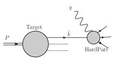
Figure 1: Illustration of DIS from a composite target ($P$) in collinear factorization, with hard scattering of a virtual photon ($q$) from an on-shell, massless parton ($\hat{k}$).

The structure tensor for the target parton in the factorized subprocess has a form similar to that of Eq. (9), but with $P^{\mu}$ replaced by $\hat{k}^{\mu}$,

$$\widehat{W}^{\mu\nu}(\hat{k},q) {}=\left(-g^{\mu\nu}+\frac{q^{\mu}q^{\nu}}{q^{2}}\right)\widehat{F}_{1}\big{(}\hat{x}_{\rm Bj}(\hat{x}_{\rm N},\hat{k}^{2}/Q^{2}),Q^{2}\big{)}$$

$${}+\left(\hat{k}^{\mu}-\frac{\hat{k}\cdot q}{q^{2}}q^{\mu}\right)\left(\hat{k}^{\nu}-\frac{\hat{k}\cdot q}{q^{2}}q^{\nu}\right)\frac{\widehat{F}_{2}\big{(}\hat{x}_{\rm Bj}(\hat{x}_{\rm N},\hat{k}^{2}/Q^{2}),Q^{2}\big{)}}{\hat{k}\cdot q}\,,$$ (24)

where $\widehat{F}_{i}$ are the corresponding structure functions for the parton. In analogy with the scaling variables for the hadron, here $\hat{x}_{\rm N}$ is the partonic version of the Nachtmann variable $x_{\rm N}$, as the natural generalization of Eq. (3),

$$\hat{x}_{\rm N}=-\frac{q^{+}}{\hat{k}^{+}}=\frac{2\hat{x}_{\rm Bj}}{1+\sqrt{1+4\hat{x}_{\rm Bj}^{2}\hat{k}^{2}/Q^{2}}}=\frac{x_{\rm N}}{\xi}\,,$$ (25)

and $\hat{x}_{\rm Bj}$ is the obvious generalization of Eq. (4),

$$\hat{x}_{\rm Bj}\equiv\frac{Q^{2}}{2\hat{k}\cdot q}=\frac{Q^{2}}{2\hat{k}^{+}q^{-}}=\frac{x_{\rm N}}{\xi}\,.$$ (26)

Since for massless partons $\hat{k}^{2}=0$, the MTA is automatic for the partonic structure tensor, and $\hat{x}_{\rm N}=\hat{x}_{\rm Bj}$. Using the notation of Eq. (20), but now for the partonic target, the partonic structure tensor can be written as

$$\widehat{W}^{\mu\nu}(\hat{k},q) {}=\left(-g^{\mu\nu}+\frac{q^{\mu}q^{\nu}}{q^{2}}\right)\widehat{\mathcal{F}}_{1}\left(\hat{x}_{\rm Bj},Q^{2}\right)$$

$${}+\left(\hat{k}^{\mu}-\frac{\hat{k}\cdot q}{q^{2}}q^{\mu}\right)\left(\hat{k}^{\nu}-\frac{\hat{k}\cdot q}{q^{2}}q^{\nu}\right)\frac{\widehat{\mathcal{F}}_{2}\left(\hat{x}_{\rm Bj},Q^{2}\right)}{\hat{k}\cdot q}\,,$$ (27)

where $\widehat{\mathcal{F}}_{i}$ are the partonic versions of the massless structure functions of Eq. (20). The factorization theorem, Eq. (1), now in terms of hadronic and partonic structure tensors, can be represented as

$$W^{\mu\nu}(P,q)=\int_{\xi_{\rm min}}^{1}\frac{\mathrm{d}\xi}{\xi}\,\widehat{W}^{\mu\nu}\big{(}\hat{k}(\xi),q\big{)}\,f(\xi)\ +\ O\left(m^{2}/Q^{2}\right)\,.$$ (28)

For brevity here we have suppressed the dependence on the renormalization group scale $Q$ in the PDF $f(\xi)$, but have included the explicit $\xi$ argument of $\hat{k}(\xi)$ to emphasize that the plus component of the target parton is related to the hadron through the momentum fraction $\xi$. Applying the projectors in Eqs. (11) allows factorization to be written in terms of structure functions, still without the MTA,

$$F_{1}\left(x_{\rm Bj}(x_{\rm N},M^{2}/Q^{2}),Q^{2}\right) {}=\int_{\xi_{\rm min}}^{1}\frac{\mathrm{d}\xi}{\xi}\,\widehat{\mathcal{F}}_{1}\big{(}\hat{x}_{\rm Bj}(\xi),Q^{2}\big{)}\,f(\xi)\,+\,O\left(m^{2}/Q^{2}\right)\,,$$ (29a)

$$F_{2}\left(x_{\rm Bj}(x_{\rm N},M^{2}/Q^{2}),Q^{2}\right) {}=\frac{Q^{2}\left(Q^{2}-M^{2}x_{\rm N}^{2}\right)}{\left(Q^{2}+M^{2}x_{\rm N}^{2}\right)^{2}}\int_{\xi_{\rm min}}^{1}\mathrm{d}\xi\,\widehat{\mathcal{F}}_{2}\big{(}\hat{x}_{\rm Bj}(\xi),Q^{2}\big{)}\,f(\xi)\,+\,O\left(m^{2}/Q^{2}\right)\,,$$ (29b)

where from Eq. (26) one has $\hat{x}_{\rm Bj}(\xi)=x_{\rm N}/\xi$. For the lower limit of the $\xi$ integration, the minimum $\xi$ occurs when $(\hat{k}+q)^{2}=0$, which gives $\xi_{\rm min}=x_{\rm N}$. Thus, without kinematical target mass approximations, the factorized expressions for the structure functions are

$$F_{1}\left(x_{\rm Bj}(x_{\rm N},M^{2}/Q^{2}),Q^{2}\right) {}=\int_{x_{\rm N}}^{1}\frac{\mathrm{d}\xi}{\xi}\,\widehat{\mathcal{F}}_{1}(x_{\rm N}/\xi,Q^{2})\,f(\xi)+O\left(m^{2}/Q^{2}\right)$$

$${}\equiv F^{\rm AOT}_{1}\left(x_{\rm Bj}(x_{\rm N},M^{2}/Q^{2}),Q^{2}\right)+O\left(m^{2}/Q^{2}\right)\,,$$ (30a)

$$F_{2}\left(x_{\rm Bj}(x_{\rm N},M^{2}/Q^{2}),Q^{2}\right) {}=\frac{Q^{2}\left(Q^{2}-M^{2}x_{\rm N}^{2}\right)}{\left(Q^{2}+M^{2}x_{\rm N}^{2}\right)^{2}}\int_{x_{\rm N}}^{1}\mathrm{d}\xi\,\widehat{\mathcal{F}}_{2}(x_{\rm N}/\xi,Q^{2})\,f(\xi)+O\left(m^{2}/Q^{2}\right)$$

$${}\equiv F^{\rm AOT}_{2}\left(x_{\rm Bj}(x_{\rm N},M^{2}/Q^{2}),Q^{2}\right)+O\left(m^{2}/Q^{2}\right)\,.$$ (30b)

The errors here arise entirely from assumptions about the smallness of intrinsic parton scales; there are no $x_{\rm Bj}^{2}M^{2}/Q^{2}$ types of errors since no MTA has been made. The second lines of Eqs. (30a) and (30b) define the “AOT structure functions”, $F^{\rm AOT}_{i}$, as the factorized structure functions with exact external kinematics Aivazis et al. (1994), and this prescription for taking target masses into account will be referred to as the AOT method. (Note that the notation in Eqs. (30) differs from that in Ref. Aivazis et al. (1994), whose focus was more on the treatment of heavy quark effects rather than on kinematical errors.) If, in addition, $x_{\rm N}$ is expanded in powers of $x_{\rm Bj}^{2}M^{2}/Q^{2}$, then Eqs. (30) become

$$F_{1}\left(x_{\rm Bj}(x_{\rm N},M^{2}/Q^{2}),Q^{2}\right) {}=\mathcal{F}_{1}(x_{\rm Bj},Q^{2})+O\left(\frac{x_{\rm Bj}^{2}M^{2}}{Q^{2}}\right)$$

$${}=\int_{x_{\rm Bj}}^{1}\frac{\mathrm{d}\xi}{\xi}\,\widehat{\mathcal{F}}_{1}(x_{\rm Bj}/\xi,Q^{2})\,f(\xi)+O\left({\rm max}\left[\frac{m^{2}}{Q^{2}}\,,\frac{x_{\rm Bj}^{2}M^{2}}{Q^{2}}\right]\right)\,,$$ (31a)

$$F_{2}\left(x_{\rm Bj}(x_{\rm N},M^{2}/Q^{2}),Q^{2}\right) {}=\mathcal{F}_{2}(x_{\rm Bj},Q^{2})+O\left(\frac{x_{\rm Bj}^{2}M^{2}}{Q^{2}}\right)$$

$${}=\int_{x_{\rm Bj}}^{1}\mathrm{d}\xi\,\widehat{\mathcal{F}}_{2}(x_{\rm Bj}/\xi,Q^{2})\,f(\xi)+O\left({\rm max}\left[\frac{m^{2}}{Q^{2}}\,,\frac{x_{\rm Bj}^{2}M^{2}}{Q^{2}}\right]\right)\,.$$ (31b)

The expressions in Eqs. (30) are the most immediate results of a factorization derivation of the style of Ref. Collins (2011), and the factorized terms on the right-hand-side can be considered nearly exact if the $m^{2}/Q^{2}$ errors (i.e., quantities like parton virtuality) are negligible. On the other hand, Eqs. (31) are the more usual way of presenting the final factorization result, which arises from applying the MTA of Sec. III to the factorized expressions in Eqs. (30). The resulting errors are suppressed by $x_{\rm Bj}^{2}M^{2}/Q^{2}$ and are here seen to be of purely kinematical origin. The approximation of dropping all power corrections in Eq. (31) and keeping only the first term on the right will be referred to as the “factorized massless target approximation” (FMTA), since it just combines standard factorization with the MTA. If we wish to keep kinematical target mass effects, we will simply maintain Eqs. (30).

In order to make the various approximations very explicit, the discussion in the last two sections of the basic theoretical set up has been much more detailed than what is usually found in the literature. This has required the introduction of a number of new notations for structure functions, which is useful to briefly summarize here:

• Hadronic structure functions, which are represented by the Roman font $F_{i}$, are functions of the independent variables $x_{\rm Bj}$ and $Q^{2}$; however, since it is ultimately convenient to express them in terms of $x_{\rm N}$ and $Q^{2}$, we write $x_{\rm Bj}$ explicitly as a function of $x_{\rm N}$ and $M^{2}/Q^{2}$ as in Eq. (9).

• The hadronic tensor can be re-expressed in a different basis of Lorentz vectors, by using $\widetilde{P}^{\mu}$ rather than $P^{\mu}$ to define the corresponding structure functions $\widetilde{F}_{i}$ in the massless basis, which we distinguish by the tilde [“  $\widetilde{}$  ”] symbol.

• When this is combined with the approximation $x_{\rm Bj}(x_{\rm N},M^{2}/Q^{2})\to x_{\rm Bj}(x_{\rm N},0)$ we obtain the $\widetilde{F}_{i}\left(x_{\rm Bj}(x_{\rm N},0),Q^{2}\right)$ structure functions evaluated as in Eq. (18).

• The script notation for the structure functions $\mathcal{F}_{i}$ is an abbreviation for the special case when $M^{2}/Q^{2}$ is set to zero in $x_{\rm Bj}(x_{\rm N},M^{2}/Q^{2})$, as in Eq. (20).

• A hat [“  $\widehat{}$  ”] on a structure function denotes a massless and on-shell partonic target. Note that structure functions in Roman font with a hat ($\widehat{F}_{i}$) and in script font with a hat ($\widehat{{\cal F}}_{i}$) are identical, since $\hat{k}^{2}=0$. Also, partonic structure functions are identical with (the partonic analogues of) either the $W^{\mu\nu}$ [Eq. (9)] or $\widetilde{W}^{\mu\nu}$ [Eq. (18)] bases, since the target parton in the hard part is always massless and on-shell.

For many subsequent practical applications some of these notations will be redundant; however, since they make the different layers of conventions and approximations very explicit, they will be useful for our present purposes.

To conclude this section, let us also summarize the key observations:

1. There are two independent types of approximations. One is the purely kinematical approximation described in Sec. III, with errors suppressed by powers of $x_{\rm Bj}^{2}M^{2}/Q^{2}$. It is independent of whatever theoretical techniques might be used to actually calculate the structure functions. The second approximation is the factorization theorem in Eq. (28), with errors suppressed by powers of $m^{2}/Q^{2}$, where $m^{2}$ is a typical scale associated with intrinsic dynamical properties of partons, such as their virtualites.

2. The MTA is not necessary for deriving collinear factorization. The relation $\hat{x}_{\rm Bj}=x_{\rm N}/\xi$ in Eq. (26) is usually automatically approximated to $x_{\rm Bj}/\xi$, but this is not needed. One may simply stop at Eqs. (30) and view the MTA application that leads to Eqs. (31) as ancillary.

3. The standard factorization derivation, as embodied in the AOT method, automatically gives $x_{\rm N}$ instead of $x_{\rm Bj}$ as the natural scaling variable for the structure functions (neglecting logarithmic $Q$ dependence from higher orders in $\alpha_{s}$).

Before concluding, let us also mention that a number of other prescriptions for dealing with the effects of a nonzero target mass on kinematics have been proposed in the literature, but generally these impose extra assumptions on the dynamics. We discuss these in more detail in Appendix A. Having reviewed the mathematical statement of factorization in the presence of target masses in detail, and the corresponding expressions for the structure functions, in the next section we turn to the question of the physical interpretation of an observed improvement from target mass effects.

V When are Target Mass Kinematics Relevant?

The most straightforward and correct approach to computing the inclusive DIS structure functions is to simply avoid introducing unnecessary kinematical errors by choosing to keep target momentum exact and applying the AOT expressions for factorization in Eqs. (30). A question of interpretation remains, however; without special knowledge of the target structure there is no reason a priori to expect the powers of $x_{\rm Bj}^{2}M^{2}/Q^{2}$ from purely kinematical approximations to be any more important than other power-suppressed corrections.

V.1 Scattering from subsystems

To interpret an observed phenomenological improvement obtained by using the AOT method instead of the FMTA, consider several generic scenarios for scattering from an extended target that could reveal a nontrivial relation between target mass effects and general properties of hadron structure. Consider, for instance, that if the target is a composite object (the precise nature of which need not be specified at this stage), then the sum of scattering amplitudes may described as occurring off subsystems of the target, as depicted in Fig. 2. We leave the nature of the dynamics completely unspecified at this stage and only assume that diagrammatic arguments apply generally. To be completely general, we also allow for the possibility that the lower (nonperturbative) blob is empty so that scattering can occur off the entire target as a whole.

To be quantitative, we define the generic subsystem to have a momentum before the collision parametrized by the four-vector

$$p=\left(XP^{+},\frac{m^{2}_{\text{T}}}{2XP^{+}},\boldsymbol{p}_{\text{T}}{}\right)\,,$$ (32)

where the squared transverse mass $m^{2}_{\text{T}}\equiv p^{2}+p^{2}_{\text{T}}$ denotes the sum of the virtuality $p^{2}$ (which could in principle be negative) and transverse momentum $p^{2}_{\text{T}}$ of the subsystem, and $X=p^{+}/P^{+}$ is the light-cone fraction of the target carried by the subsystem. The collision with the exchanged virtual photon produces another system of particles with invariant mass-squared

$$v^{2}\equiv(p+q)^{2}\,.$$ (33)

Such a system need not be physical and could be off-shell; for example, it could be a part of a hadronizing string. Without loss of generality, we may describe the total lepton scattering amplitude for the whole target $\mathcal{A}^{\rm tot}(P,q,l^{\prime})$, which in general depends on three variables (chosen here to be $P$, $q$ and $l^{\prime}$), in terms of the amplitude for scattering off the subsystem,

$$\mathcal{A}^{p}(p,q,l^{\prime}).$$

To connect to the total amplitude $\mathcal{A}^{\rm tot}$, the subsystem amplitude needs to be integrated over all components of $p$, weighted by a function that characterizes the four-momentum distribution of the subsystem in the overall target.

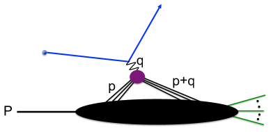
Figure 2: DIS from a subsystem ($p$) of a composite target ($P$). The solid lines connecting to the virtual photon ($q$) through the upper blob can be any constituents of the target.

To avoid confusion in what follows below, it is important not to view the diagram in Fig. 2 as the sort of “region” diagram common in factorization derivations Collins (2011), but rather as a topological representation in which the blobs are not necessarily characterized by any particular (small or large) momentum. The blobs simply denote an arbitrary subgraph assignment for some graphical contribution to the amplitude; some lines are routed through the (upper) photon–subsystem part of the graph, while others are diverted through the (lower) part of the graph connected to the target.

Such organization does not achieve much of interest until we pose questions about possible relationships between the total target and subsystem momenta, $P$ and $p$. If we find that there is an assignment in Fig. 2 such that $p^{2}_{\text{T}},m^{2}_{\text{T}}\ll Q^{2}$ for typical values of $p^{2}_{\text{T}}$ and $m^{2}_{\text{T}}$, then up to power-suppressed errors the amplitude for scattering from the subsystem becomes a function of $X$ only,

$$\mathcal{A}^{p}(p,q,l^{\prime})=\mathcal{A}^{p}(X,q,l^{\prime})+O\left(\frac{m^{2}}{Q^{2}}\right)\,,$$ (34)

where $m^{2}$ refers to $p^{2}_{\text{T}}$ or $m^{2}_{\text{T}}$. The entire factorization derivation can then be performed for the sub-amplitude $\mathcal{A}^{p}(X,q,l^{\prime})$ rather than for the total amplitude $\mathcal{A}^{\rm tot}(P,q,l^{\prime})$.

In general the invariant mass $v^{2}$ varies between small values ($\approx 0$) and large values (of order $Q^{2}$ or larger). In the standard QCD factorization paradigm, large-$v^{2}$ behavior is describable by perturbative calculations. One can therefore define an approximate invariant mass squared $\tilde{v}^{2}$ of the final state subsystem which is calculated by approximate methods that deal with values of $v^{2}/Q^{2}=O\left(1\right)$,

$$v^{2}\equiv\tilde{v}^{2}+\delta v^{2},$$ (35)

where $\delta v^{2}$ is the correction needed to recover the exact $v^{2}$ value. The approximate invariant mass squared $\tilde{v}^{2}$ may vary from zero to $O\left(Q^{2}\right)$, while $\delta v^{2}$ is of the order of a typical small scale comparable to $p^{2}_{\text{T}}$ and $m^{2}_{\text{T}}$. Expanding $X$ in terms of these variables, we can write

$$X =x_{\rm N}\left\{1+\frac{\tilde{v}^{2}}{Q^{2}}+\frac{p^{2}_{\text{T}}+\delta v^{2}}{Q^{2}}-\frac{m^{2}_{\text{T}}(p^{2}_{\text{T}}+\tilde{v}^{2}+\delta v^{2})}{Q^{4}}+\cdots\right\},$$ (36a)

and, further expanding the Nachtmann variable $$x_{\rm N}$$, the light-cone fraction becomes

$$X =x_{\rm Bj}\left\{1+\frac{\tilde{v}^{2}}{Q^{2}}+\frac{p^{2}_{\text{T}}+\delta v^{2}-x_{\rm Bj}^{2}M^{2}}{Q^{2}}-\frac{(m^{2}_{\text{T}}+x_{\rm Bj}^{2}M^{2})(p^{2}_{\text{T}}+\tilde{v}^{2}+\delta v^{2})-2x_{\rm Bj}^{4}M^{4}}{Q^{4}}+\cdots\right\}\,.$$ (36b)

If the typical values of small mass scales associated with the interactions between subsystems ($p^{2}_{\text{T}}$, $m^{2}_{\text{T}}$ and $\delta v^{2}$) are totally negligible, but $x_{\rm Bj}^{2}M^{2}$ is comparatively large, then the expansion in Eq. (36a) is an improvement over the expansion in Eq. (36b). In other words, in the limit of large $Q$,

$$X\ \approx\ x_{\rm N}\left(1+\frac{\tilde{v}^{2}}{Q^{2}}\right)\,$$ (37a)

provides a better approximation than

$$\ \ X\ \approx\ x_{\rm Bj}\left(1+\frac{\tilde{v}^{2}}{Q^{2}}\right)\,.$$ (37b)

In both of these cases, the connection between $X$ and external observables has lost any sensitivity to the details of interactions between subsystems. The only dependence on dynamics is through $\tilde{v}^{2}$, which is calculable in factorization and perturbation theory. Suggestively defining

$$\left(1+\frac{\tilde{v}^{2}}{Q^{2}}\right)\,\equiv\,\frac{1}{\xi}\,,$$ (38)

the subsystem amplitude in Eq. (34) can be written

$$\mathcal{A}^{p}(p,q,l^{\prime}) {}=\mathcal{A}^{p}(x_{\rm N}/\xi,q,l^{\prime})+O\left(\frac{m^{2}}{Q^{2}}\right)\,$$ (39a)

$${}=\mathcal{A}^{p}(x_{\rm Bj}/\xi,q,l^{\prime})+O\left({\rm max}\left[\frac{m^{2}}{Q^{2}}\,,\frac{x_{\rm Bj}^{2}M^{2}}{Q^{2}}\right]\right)\,.$$ (39b)

If $x_{\rm Bj}^{2}M^{2}\sim Q^{2}$ but $p^{2}_{\text{T}},m^{2}_{\text{T}},\delta v^{2}\ll Q^{2}$, then truncating the expansion in (39a) is valid while in (39b) it is not. If, however, $x_{\rm Bj}^{2}M^{2}\sim p^{2}_{\text{T}},m^{2}_{\text{T}},\delta v^{2}$, then there is no reason to expect either expansion to be any better or worse than the other. The same statements apply to the overall cross section, since it is related to $\mathcal{A}^{p}$ by taking the square modulus, summing over hadronic final states, and integrating over $\boldsymbol{p}_{\text{T}}{}$ and $m_{\rm T}$ (whose typical values are restricted by the $p^{2}_{\text{T}},m^{2}_{\text{T}}\ll Q^{2}$ assumption to be small and are thus decoupled from $\mathcal{A}^{p}$).

The above discussion naturally leads us to the conclusion that, if $x_{\rm Bj}^{2}M^{2}$ is large but subsystem scales are small, then the cross section reduces to a function of $x_{\rm N}/\xi$, with the momentum fraction $\xi$ calculable from methods that account for large $\tilde{v}^{2}$ — all of which can be performed within standard factorization. The AOT set of expressions [Eqs. (30)] is just a specific realization of this within collinear factorization. Namely, the hard scattering subprocess is always a function of $x_{\rm N}$, while large final state invariant masses in the hard part of the scattering amplitude are accounted for by using $x_{\rm N}/\xi$ in the subprocess, with $\xi$ obtained as in Eqs. (37). In other words, if the typical $|p^{2}|$ is small and $p$ is collinear to $P$, then the steps for deriving factorization can be applied directly to $|\mathcal{A}^{p}(p,q,l^{\prime})|^{2}$ with $p^{2}=0$ rather than to $|\mathcal{A}^{\rm tot}(P,q,l^{\prime})|^{2}$. The result is automatically the AOT factorization in Eqs. (30). Furthermore, since it accounts for large $\tilde{v}^{2}$, the AOT improvement applies to all orders in perturbation theory.

V.2 TMC improvement and hierarchy of scales

Now we may ask what general characteristics of a composite target can give rise to a scenario where $p^{2}_{\text{T}},m^{2}_{\text{T}}\ll x_{\rm Bj}^{2}M^{2}$, which would justify the result in Eq. (39a) being an improvement over that in Eq. (39b). At one extreme, it cannot be the case of scattering from a single, isolated perturbative quark or gluon, as these can emit large amounts of collinear and soft radiation. Moreover, a perturbative quark has virtuality that ranges up to $O\left(Q^{2}\right)$. A system of collinearly propagating quarks and gluons that are nearly massless and on-shell cannot be described purely in terms of short-distance, perturbative propagators. At the other extreme, the $p^{2}_{\text{T}},m^{2}_{\text{T}}\ll x_{\rm Bj}^{2}M^{2}$ condition also cannot arise when all or most of the lines in Fig. 2 are routed through the upper part of the diagram, leaving the blob in the lower part of the diagram completely empty, which would correspond to $m_{\rm T}\sim M$.

The only way, therefore, to consistently arrive at a scenario whereby $p^{2}_{\text{T}},m^{2}_{\text{T}}\ll x_{\rm Bj}^{2}M^{2}$, and thus Eq. (39a) (in terms of $x_{\rm N}$) be an improvement over Eq. (39b) (in terms of $x_{\rm Bj}$), is if the target consists of more than one separate, low-invariant mass (relative to $x_{\rm Bj}^{2}M^{2}$) subsystem that can play the role of the lines entering the upper blob in Fig. 2. To avoid pushing $|p^{2}|$ too high, the interactions between subsystems need to be reasonably weak. While the individual subsystems necessarily need to have a small typical invariant mass $|p^{2}|$ relative to $x_{\rm Bj}^{2}M^{2}$, each subsystem can involve internal interactions that involve scales much larger than $p^{2}_{\text{T}},m^{2}_{\text{T}},\delta v^{2}$, but still much smaller than $Q^{2}$. Therefore, it is only the scales involved in the interactions between subsystems that need to be very small in order for the above argument for the usefulness of the AOT method to be valid.

Our general conclusion is that any observed improvement in the theoretical description of scattering that comes from using Eq. (39a) instead of Eq. (39b) is suggestive of a hierarchy of “clustered” structures within the target, representing correlated subsystems of strongly interacting particles. We stress that we are totally agnostic about what those clusters might be; our observation is simply that, kinematically, some sort of clustering is preferred. Thus, an improvement in the phenomenological description using the AOT method can be interpreted as evidence that scattering occurs off a collection of weakly interacting subsystems (since $p^{2}_{\text{T}}$, $m^{2}_{\text{T}}$ and $\delta v^{2}$ must be small relative to $x_{\rm Bj}^{2}M^{2}$), while a failure to observe any improvement suggests a more complicated type of scattering. (Some of this also echoes earlier discussions of TMCs in DIS at low energies, such as in Ref. De Rújula et al. (1977a), see pg. 325, where the scale $M_{0}$ there is analogous to the mass $m$ used in the present work.) A subsystem can in general be any nonperturbative system, consisting of one or more interacting particles, whose internal interactions are stronger than interactions with other subsystems in the target. The subsystem could, for example, be colored or colorless; for the latter, we notice that for a nucleon target the region of kinematics where the $x_{\rm Bj}^{2}M^{2}/Q^{2}$ corrections are important corresponds to the nucleon resonance region, and the subsystems might be a collection of hadrons, such as nucleons and pions. However, the exact nature of the target or its subsystems and their interactions is not relevant to our discussion.

The above argument is very general, since it only relies on the kinematics of scattering off subsystems in a target, and the assumption that scattering from the composite object can be described in generally diagrammatic terms. In particular, it applies to arbitrary orders in perturbation theory. In fact, arriving at Eqs. (39) does not even require factorization or partonic degrees of freedom specifically. It only states that, if scattering occurs off weakly interacting light and nearly on-shell subsystems in a heavier target, then the cross section at a particular $v^{2}$ becomes a function of $x_{\rm N}/\xi$, where $\xi$ is either 1 or is obtainable from large-$\tilde{v}^{2}$ methods.

An example of such a scale hierarchy could be nuclear targets, where the subsystems correspond to nucleons; the hierarchy arises because interactions between nucleons are much weaker than the typical interactions binding quarks and gluons inside the nucleons Geesaman et al. (1995); Malace et al. (2014). Other examples may be nucleons coupled to soft pseudoscalar mesons through chiral dynamics, which can give rise to unique nonperturbative features in sea quarks in the proton Thomas (1983); Signal and Thomas (1987); Salamu et al. (2015); Wang et al. (2016); Geesaman and Reimer (2018). A possible hierarchy with explicit color degrees of freedom could involve partons clustered into constituent quark-like subsystems Close (1979); Richard (2012). Conversely, an example of a target where one would not expect an improvement would be the case of a hadron target whose mass comes almost entirely from a single point-like quark, such as a heavy quark hadron. We stress again, however, that our arguments here do not rely on any assumptions about dynamics of the composite object or the nature of its subsystems, but only on the kinematical considerations associated with target mass improvement.

VI Conclusion

In this paper we have presented a detailed description of the basic structure function analysis of deeply inelastic scattering in the context of QCD factorization, fully taking into account hadronic masses in order to give clarity to the notion of “purely kinematical” mass effects. Even when clearly stated, however, the meaning of an improvement in the theoretical description of the scattering process from purely kinematical effects of the target mass begs for a physical interpretation.

The discussions in Secs. III–V make clear that an improvement is natural if factorization is understood to apply to scattering off a small invariant mass subsystem or cluster inside a composite target. Models of the nucleon with multiple scales and a clustering structure imply a particular kind of phenomenological prediction — that standard collinear QCD factorization, in the form of AOT framework for treating target masses with exact external kinematics, can be extended to smaller $Q$ and larger $x_{\rm Bj}$ than might otherwise be expected from perturbative QCD arguments. In the limit of large $Q$, with all other scales fixed, and assuming $x_{\rm Bj}M\approx Q$, it is the first terms on the right hand sides of Eqs. (30a) and (30b) that give the asymptotic behavior. The clustering hypothesis suggests that, as $Q$ decreases, the power corrections initially come mainly from switching between $x_{\rm Bj}$ and $x_{\rm N}$ in the usual factorized expressions, and also accounting for overall kinematic factors such as in Eq. (30b).

An interesting consequence is that the degree of purely kinematical improvement found by keeping the target mass can be viewed as probing the degree of clustering in the target. To quantify this, it will be interesting to investigate how much improvement can be expected within specific models of the target. This way of viewing the target mass effects suggests a variety of future directions for research.

From phenomenological and global QCD analyses of deep inelastic lepton–nucleon scattering data, it is already well established that treatments of the target mass that switch $x_{\rm Bj}$ to $x_{\rm N}$ significantly improve the description of the data and extend its range to lower $Q$ and larger $x_{\rm Bj}$ values De Rújula et al. (1977a); Ji and Unrau (1995); Bianchi et al. (2004); Accardi et al. (2010); Owens et al. (2013); Kulagin and Sidorov (2000); Alekhin et al. (2017); Accardi et al. (2016). On the other hand, clear room for refinement exists, for example to distinguish between precise implementations of TMCs that have been proposed in the literature Georgi and Politzer (1976); Barbieri et al. (1976); Ellis et al. (1983); Isgur et al. (2001); Steffens and Melnitchouk (2006); Schienbein et al. (2008); Accardi and Qiu (2008); Brady et al. (2011); Steffens et al. (2012). Also, upcoming experiments will allow for comparison between different target structures, including pions, kaons, and nuclei Arrington et al. (2001, 2006); Melnitchouk (2003); Melnitchouk et al. (2005). While the discussion in the present work has for simplicity been restricted to a single flavor, the generalization to the more realistic case of multiple flavors is straightforward. Moreover, the treatment of structure functions in Secs. II through IV can be directly extended to spin and polarization dependent structure functions. This will be important since the extraction of certain spin dependent effects can be especially sensitive to target mass effects Wandzura (1977); Matsuda and Uematsu (1980); Piccione and Ridolfi (1998); Blümlein and Tkabladze (1999); Bosted et al. (2007); Solvignon et al. (2008). We leave these interesting and important topics for future consideration.

Appendix A Contrast with other TMC methods

Throughout this paper we have adopted what could be viewed as the most natural meaning of a “purely kinematical correction”; namely, a correction that is totally independent of any assumptions pertaining to the dynamics within the target. The MTA from Sec. III accounts for all such approximations that one encounters in the context of standard collinear factorization in DIS. The purely kinematical target mass correction is therefore uniquely of the form derived by AOT Aivazis et al. (1994) (see Sec. IV), since this is merely the combination of the MTA and standard factorization, which is independent of target mass kinematics. Any other corrections must involve at least some set of additional assumptions about parton dynamics.

In the literature there exist a number of other prescriptions that are sometimes described as “purely kinematical” target mass corrections, but which in various ways differ from the AOT approach. Probably the best known of these is the treatment by Georgi and Politzer Georgi and Politzer (1976) based on the operator product expansion (OPE). (For extensions to the polarized case see Refs. Wandzura (1977); Matsuda and Uematsu (1980); Piccione and Ridolfi (1998); Blümlein and Tkabladze (1999).) Here the expressions for target mass corrected structure functions contain extra terms involving integrals of structure functions, which arise from additional constraints or assumptions that are beyond the purely kinematical corrections implicit in the AOT approach. As discussed by Ellis, Furmanski and Petronzio Ellis et al. (1983), and more recently by D’Alesio, Leader and Murgia D’Alesio et al. (2010), the origin of the additional integral factors is the constraint that the struck partons inside the target correlation function should be exactly massless and on-shell, for all longitudinal momenta and for all transverse momenta. Absent some exotic dynamical mechanisms within the target, this appears to be a relatively strong assumption, which in itself is not a necessary one for the standard derivation of collinear factorization.

Another way to understand the difference between the AOT approach and the OPE-based prescription is to note that in the latter the kinematical TMCs that are kept are only those that are relevant for a leading twist treatment, while kinematical corrections associated with higher twists are neglected. This type of assessment of $O\left(m^{2}/Q^{2}\right)$-type errors runs the risk of entangling the $O\left(x_{\rm Bj}^{2}M^{2}/Q^{2}\right)$ target mass corrections with those from other sources. By refraining from introducing $O\left(x_{\rm Bj}^{2}M^{2}/Q^{2}\right)$-type errors from the outset, the direct method used by AOT has the advantage of including all kinematical target mass effects regardless of twist. It is worth emphasizing here that modern derivations of factorization do not need to use the OPE, but rather can be formulated as direct, arbitrary-order expansions in powers of $1/Q^{2}$ Collins (2011). An added benefit of the direct method, which can be argued to be the more rigorous one, is that it does not a priori need to entail an MTA.

Still other TMC formalisms have been proposed that also differ from, or go beyond, AOT Ellis et al. (1983); Accardi and Qiu (2008). For example, the Accardi-Qiu prescription Accardi and Qiu (2008) uses collinear factorization together with the dynamical assumptions that well-defined target and jet directions exist at rather low $Q^{2}$ Accardi and Signori (2018); Sterman (1987) and that the initial state baryon number flows only along one such direction Guerrero and Accardi (2018). This relies on a very literal matching between virtual partonic states and a particular final state distribution of hadrons, which goes beyond the standard factorization paradigm Collins et al. (1988); Collins (2011) but regulates the behavior near the kinematical threshold at $x_{\rm Bj}=1$.

The direct factorization approach can also help to contextualize the so-called “threshold problem” Georgi and Politzer (1976), which is the observation that the structure function for nonzero target mass in the OPE derivation has support at $x_{\rm Bj}=1$ (where kinematically only elastic scattering should contribute) and can be nonzero in the unphysical region $x_{\rm Bj}>1$ (up to $x_{\rm N}=1$) De Rújula et al. (1977b). This has led to various proposals for modifying the target mass corrected structure functions such that they have support only in the physical region De Rújula et al. (1977b); Johnson and Tung (1979); Bitar et al. (1979); Steffens and Melnitchouk (2006); Steffens et al. (2012); D’Alesio et al. (2010). The solution to the “threshold problem” from the factorization perspective is simply that the conditions for which QCD factorization itself is valid break down as $x_{\rm Bj}\to 1$. While the structure functions are defined through Eq. (10) for all $x_{\rm Bj}\leq 1$, and the parton distribution $f(\xi)$ exists for all parton momentum fractions $\xi\in[0,1]$, the factorization formulas in Eqs. (28) and (30) relating the two receive increasingly large corrections at large $x_{\rm Bj}$ that render the perturbative expansion in powers of both $\alpha_{s}$ and $1/Q^{2}$ no longer a useful one. Improvements beyond this require more sophisticated methods for treating the large-$x_{\rm Bj}$ region than what is available in the standard factorization treatment.

References

- Collins et al. (1988) J. C. Collins, D. E. Soper, and G. Sterman, Adv. Ser. Direct. High Energy Phys. 5, 1 (1988), hep-ph/0409313 .
- Bloom and Gilman (1971) E. D. Bloom and F. J. Gilman, Phys. Rev. D 4, 2901 (1971).
- De Rújula et al. (1977a) A. De Rújula, H. Georgi, and H. D. Politzer, Annals Phys. 103, 315 (1977a).
- Poggio et al. (1976) E. C. Poggio, H. R. Quinn, and S. Weinberg, Phys. Rev. D 13, 1958 (1976).
- Ji and Unrau (1995) X. Ji and P. Unrau, Phys. Rev. D 52, 72 (1995).
- Melnitchouk et al. (2005) W. Melnitchouk, R. Ent, and C. Keppel, Phys. Rep. 406, 127 (2005).
- Duke and Roberts (1980) D. W. Duke and R. G. Roberts, Nucl. Phys. B166, 243 (1980).
- Devoto et al. (1983) A. Devoto, D. W. Duke, J. F. Owens, and R. G. Roberts, Phys. Rev. D 27, 508 (1983).
- Christy and Melnitchouk (2011) M. E. Christy and W. Melnitchouk, J. Phys. Conf. Ser. 299, 012004 (2011).
- Chen et al. (2011) J. P. Chen, A. Deur, S. Kuhn, and Z. E. Meziani, J. Phys. Conf. Ser. 299, 012005 (2011).
- Gilman et al. (2011) R. Gilman, R. J. Holt, and P. Stoler, J. Phys. Conf. Ser. 299, 012009 (2011).
- Collins (2011) J. C. Collins, Foundations of Perturbative QCD (Cambridge University Press, Cambridge, 2011).
- Ellis et al. (1996) R. K. Ellis, W. J. Stirling, and B. R. Webber, Camb. Monogr. Part. Phys. Nucl. Phys. Cosmol. 8, 1 (1996).
- Nachtmann (1973) O. Nachtmann, Nucl. Phys. B63, 237 (1973).
- Aivazis et al. (1994) M. A. G. Aivazis, F. I. Olness, and W.-K. Tung, Phys. Rev. D 50, 3085 (1994).
- Greenberg and Bhaumik (1971) O. W. Greenberg and D. Bhaumik, Phys. Rev. D4, 2048 (1971).
- Kretzer and Reno (2002) S. Kretzer and M. H. Reno, Phys. Rev. D 66, 113007 (2002).
- Schienbein et al. (2008) I. Schienbein et al., J. Phys. G 35, 053101 (2008).
- Accardi and Qiu (2008) A. Accardi and J. Qiu, JHEP 07, 090 (2008).
- Brady et al. (2011) L. T. Brady, A. Accardi, T. J. Hobbs, and W. Melnitchouk, Phys. Rev. D 84, 074008 (2011).
- Geesaman et al. (1995) D. F. Geesaman, K. Saito, and A. W. Thomas, Ann. Rev. Nucl. Part. Sci. 45, 337 (1995).
- Malace et al. (2014) S. Malace, D. Gaskell, D. W. Higinbotham, and I. Cloet, Int. J. Mod. Phys. E 23, 1430013 (2014).
- Thomas (1983) A. W. Thomas, Phys. Lett. 126B, 97 (1983).
- Signal and Thomas (1987) A. I. Signal and A. W. Thomas, Phys. Lett. B 191, 205 (1987).
- Salamu et al. (2015) Y. Salamu, C.-R. Ji, W. Melnitchouk, and P. Wang, Phys. Rev. Lett. 114, 122001 (2015).
- Wang et al. (2016) X. G. Wang, C.-R. Ji, W. Melnitchouk, Y. Salamu, A. W. Thomas, and P. Wang, Phys. Rev. D 94, 094035 (2016).
- Geesaman and Reimer (2018) D. F. Geesaman and P. E. Reimer, (2018), arXiv:1812.10372 [nucl-ex] .
- Close (1979) F. E. Close, An Introduction to Quarks and Partons (Academic Press, London, 1979).
- Richard (2012) J.-M. Richard, in Ferrara International School Niccolò Cabeo 2012: Hadronic Spectroscopy (2012) arXiv:1205.4326 [hep-ph] .
- Bianchi et al. (2004) N. Bianchi, A. Fantoni, and S. Liuti, Phys. Rev. D 69, 014505 (2004).
- Accardi et al. (2010) A. Accardi, M. E. Christy, C. E. Keppel, P. Monaghan, W. Melnitchouk, J. G. Morfin, and J. F. Owens, Phys. Rev. D 81, 034016 (2010).
- Owens et al. (2013) J. Owens, A. Accardi, and W. Melnitchouk, Phys. Rev. D 87, 094012 (2013).
- Kulagin and Sidorov (2000) S. A. Kulagin and A. V. Sidorov, Eur. Phys. J. A 9, 261 (2000).
- Alekhin et al. (2017) S. I. Alekhin, S. A. Kulagin, and R. Petti, Phys. Rev. D 96, 054005 (2017).
- Accardi et al. (2016) A. Accardi, L. T. Brady, W. Melnitchouk, J. F. Owens, and N. Sato, Phys. Rev. D 93, 114017 (2016).
- Georgi and Politzer (1976) H. Georgi and H. D. Politzer, Phys. Rev. D 14, 1829 (1976).
- Barbieri et al. (1976) R. Barbieri, J. R. Ellis, M. K. Gaillard, and G. G. Ross, Nucl. Phys. B117, 50 (1976).
- Ellis et al. (1983) R. K. Ellis, W. Furmanski, and R. Petronzio, Nucl. Phys. B212, 29 (1983).
- Isgur et al. (2001) N. Isgur, S. Jeschonnek, W. Melnitchouk, and J. W. Van Orden, Phys. Rev. D 64, 054005 (2001).
- Steffens and Melnitchouk (2006) F. M. Steffens and W. Melnitchouk, Phys. Rev. D 73, 055202 (2006).
- Steffens et al. (2012) F. M. Steffens, M. D. Brown, W. Melnitchouk, and S. Sanches, Phys. Rev. C86, 065208 (2012).
- Arrington et al. (2001) J. Arrington et al., Phys. Rev. D 64, 014602 (2001).
- Arrington et al. (2006) J. Arrington, R. Ent, C. E. Keppel, J. Mammei, and I. Niculescu, Phys. Rev. D 73, 035205 (2006).
- Melnitchouk (2003) W. Melnitchouk, Phys. Rev. D 67, 077502 (2003).
- Wandzura (1977) S. Wandzura, Nucl. Phys. B122, 412 (1977).
- Matsuda and Uematsu (1980) S. Matsuda and T. Uematsu, Nucl. Phys. B168, 181 (1980).
- Piccione and Ridolfi (1998) A. Piccione and G. Ridolfi, Nucl. Phys. B513, 301 (1998).
- Blümlein and Tkabladze (1999) J. Blümlein and A. Tkabladze, Nucl. Phys. B553, 427 (1999).
- Bosted et al. (2007) P. E. Bosted et al., Phys. Rev. C 75, 035203 (2007).
- Solvignon et al. (2008) P. Solvignon et al., Phys. Rev. Lett. 101, 182502 (2008).
- D’Alesio et al. (2010) U. D’Alesio, E. Leader, and F. Murgia, Phys. Rev. D 81, 036010 (2010).
- Accardi and Signori (2018) A. Accardi and A. Signori, PoS DIS2018, 158 (2018), arXiv:1808.00565 [hep-ph] .
- Sterman (1987) G. F. Sterman, Nucl. Phys. B281, 310 (1987).
- Guerrero and Accardi (2018) J. V. Guerrero and A. Accardi, Phys. Rev. D 97, 114012 (2018).
- De Rújula et al. (1977b) A. De Rújula, H. Georgi, and H. D. Politzer, Phys. Rev. D 15, 2495 (1977b).
- Johnson and Tung (1979) P. W. Johnson and W.-K. Tung, in 7th International Conference on Neutrinos, Weak Interactions and Cosmology – Neutrino ’79, Bergen, Norway (1979).
- Bitar et al. (1979) K. Bitar, P. W. Johnson, and W.-K. Tung, Phys. Lett. B 83, 114 (1979).