Constraining the neutral fraction of hydrogen in the IGM at redshift 7.5

Abstract

We present a large spectroscopic campaign with Keck/MOSFIRE targeting Lyman-alpha emission (Ly$\alpha$) from intrinsically faint Lyman-break Galaxies (LBGs) behind 12 efficient galaxy cluster lenses. Gravitational lensing allows us to probe the more abundant faint galaxy population to sensitive Ly$\alpha$ equivalent width limits. During the campaign we targeted 70 LBG candidates with MOSFIRE Y-band, selected photometrically to cover Ly$\alpha$ over the range $7<z<8.2$. We detect $S/N>5$ emission lines in 2 of these galaxies and find that they are likely Ly$\alpha$ at $z=7.148\pm 0.001$ and $z=7.161\pm 0.001$. We present new lens models for 4 of the galaxy clusters, using our previously published lens models for the remaining clusters to determine the magnification factors for the source galaxies. Using a Bayesian framework that employs large scale reionization simulations of the intergalactic medium (IGM) as well as realistic properties of the interstellar medium and circumgalactic medium, we infer the volume-averaged neutral hydrogen fraction, $\overline{x}_{\mathrm{HI}}$, in the IGM during reionization to be $\overline{x}_{\mathrm{HI}}=0.88^{+0.05}_{-0.10}$ at $z=7.6\pm 0.6$. Our result is consistent with a late and rapid reionization scenario inferred by Planck.

1. Introduction

The Epoch of Reionization is a significant gap in our understanding of cosmic history. In recent decades it has been the subject of intensive observational campaigns spanning the entire electromagnetic spectrum. A first step in understanding reionization is constraining the timeline, which will provide a link between the well-studied ionized universe at $z\lesssim 6$ with the Dark Ages, the period of time after Recombination ($z\lesssim 1100$) but before the first sources of light emerged ($z\gtrsim 20$). Knowledge of the timeline will help to constrain the abundance and properties of the sources driving reionization, potentially solving the longstanding debate as to whether quasars or galaxies are the primary sources (e.g. Haiman & Loeb, 1998; Madau et al., 1999). If quasars are primarily responsible, they must exist in greater numbers than the current high-redshift quasar luminosity function suggests (Onoue et al., 2017; McGreer et al., 2018).

Galaxies are more promising sources as they exist in far greater numbers than quasars. The faint-end slope of the galaxy luminosity function suggests that faint galaxies may provide far more ionizing photons beyond the current detection limit, provided ionizing photon production efficiencies and escape fractions do not decline with luminosity (e.g. Finkelstein et al., 2015; Bouwens et al., 2015a; Livermore et al., 2017; Bouwens et al., 2017). Furthermore, Bouwens et al. (2015a) found that the redshift evolution of the ionizing emissivity required to produce the Thomson optical depth measured by Planck Collaboration et al. (2016a) approximately matched the redshift evolution of the galaxy luminosity density.

The first observational evidence for reionization was the detection of a Gunn & Peterson (1965) trough in a quasar at $z=6.28$ (Becker et al., 2001). By compiling observations of $\sim 20$ quasars at $z\sim 6$, Fan et al. (2006) found that at $z\lesssim 6$, reionization had likely concluded. The “instantaneous” redshift of reionization has also been constrained via the Cosmic Microwave Background anisotropy from both WMAP (Hinshaw et al., 2013) and Planck (Planck Collaboration et al., 2016b), with some tension between the two. Planck Collaboration et al. (2016b) measured this redshift to lie in the interval $z=7.8-8.8$, lower than the WMAP measurement of $z=9.5-11.7$ (Hinshaw et al., 2013).

In the last decade, many techniques have been developed to probe the state of reionization via the volume-averaged neutral hydrogen fraction ($\overline{x}_{\mathrm{HI}}$) in the inter-galactic medium (IGM), which must evolve from $\overline{x}_{\mathrm{HI}}$=$1$ before reionization to $\overline{x}_{\mathrm{HI}}$$\simeq 0$ after reionization is complete. Quasars are often used in this approach due to their intrinsic brightness, which allows them to be observed at very high redshift (e.g. McGreer et al., 2015; Greig et al., 2017; Bañados et al., 2018). However, their rarity is a limitation in this application, especially considering each quasar only probes a single line of sight through the universe.

A complementary approach is to observe the Lyman-alpha (Ly$\alpha$, rest-frame $1216$Å) line from a large sample of galaxies. Ly$\alpha$ is a strong rest-frame ultraviolet (UV) emission line that is redshifted to near-infrared wavelengths for sources at the Epoch of Reionization ($z\gtrsim 6$), Ly$\alpha$ photons are easily absorbed by neutral hydrogen, making the line a sensitive probe of the state of the IGM during reionization. The “Ly$\alpha$ fraction” test (e.g. Stark et al., 2010; Pentericci et al., 2011), i.e. measuring the fraction of Lyman Break Galaxies with detected Ly$\alpha$ as a way to constrain the Ly$\alpha$ optical depth, is one such technique. This kind of test has been carried out by several teams, confirming a decline in the fraction of LBGs that show Ly$\alpha$ emission above a rest-frame equivalent width of $\mathrm{EW_{Ly\alpha}}=25$ Å from $z=6$ to $z=7$, consistent with an increase in Ly$\alpha$ optical depth (e.g. Fontana et al., 2010; Stark et al., 2011; Pentericci et al., 2011; Schenker et al., 2012; Ono et al., 2012; Treu et al., 2012; Tilvi et al., 2014; Pentericci et al., 2014; Schenker et al., 2014), and thus an increase in the neutral hydrogen fraction over the same interval. An important difference between the Ly$\alpha$ fraction test and the Gunn-Peterson trough constraint is the fact that the Ly$\alpha$ transmission at $z>6$ is small but non-zero. This allows the test to be meaningfully extended to higher redshift. Due to the large abundance of galaxies, the test can also be binned more finely, enabling a more detailed evolutionary study and therefore insight into the evolution of the properties of the sources of ionizing photons.

Despite these advantages, measuring the Ly$\alpha$ optical depth does not directly constrain $\overline{x}_{\mathrm{HI}}$. One must make assumptions regarding the distribution of the neutral and ionized gas within the interstellar media (ISM) and circumgalactic media (CGM) of the galaxies themselves because Ly$\alpha$ can be highly attenuated before it enters the IGM. Furthermore, the large-scale structure of the IGM during reionization can affect the inference on the neutral fraction inferred from Ly$\alpha$ surveys.

Treu et al. (2012, 2013) suggested that using the full Ly$\alpha$ equivalent width distribution, rather then the fraction of detections at some fixed arbitrary threshold, vastly improves the information content on the distribution of Ly$\alpha$ optical depth, and thus in turn on the neutral fraction, provided that the effects of the ISM and IGM can be isolated. Mesinger et al. (2015) put forward a model that ties observations of Ly$\alpha$ to large-scale reionization simulations of the IGM. Mason et al. (2018a) built on the Bayesian framework introduced by Treu et al. (2012, 2013) and the simulations by Mesinger et al. (2015), adding empirical models of the effects of the ISM and CGM, to develop a complete end-to-end inference from Ly$\alpha$ observations to the hydrogen neutral fraction.

In this paper, we make use of the Mason et al. (2018a) models to infer the neutral hydrogen fraction at $z\sim 7.5$ from a Ly$\alpha$ spectroscopic campaign with the Multi-Object Spectrometer for InfraRed Exploration (MOSFIRE; McLean et al., 2010). Our spectroscopic campaign was designed to target 12 galaxy clusters, comprising some of the best gravitational lenses in terms of number of magnified high-$z$ galaxies. The galaxy clusters act as cosmic telescopes, magnifying the background galaxies. This allows us to probe the sub-$L_{\star}$ galaxy population, which likely comprises more typical regions of the universe at $z>7$ than the $\gtrsim L_{\star}$ population. Using 12 galaxy cluster fields also allows us to mitigate cosmic variance by probing multiple independent lines of sight.

In Section 2, we present our imaging and spectroscopic data. We present our main results in Section 3, including the sample of high-z galaxies in Section 3.1, gravitational lens models in Section 3.2, the search for Ly$\alpha$ in Sections 3.3, Ly$\alpha$ detections in Section 3.4, analysis of non-detections in Section 3.6, and the neutral fraction inference in Section 3.7. We discuss the neutral fraction result and its implication on the reionization timeline in Section 4. We summarize our results in Section 5. Throughout this work, we adopt the following cosmology: $\Omega_{m}=0.3$, $\Omega_{\Lambda}=0.7$ and $h=0.7$. All magnitudes are given in the AB system, all dates are given in UTC, and all uncertainties are $68\%$ confidence unless specified otherwise.

2. Data

Here we describe the spectroscopic and imaging data that we used in this work. We also describe the photometric pipeline we use to create source catalogs from the reduced images.

2.1. Spectroscopic Data Reduction and Calibration

Table 1MOSFIRE slit-masks targeted

Cluster	mask name	date of observation	$t_{\mathrm{exp}}$	$<\mathrm{seeing}>$	$<\mathrm{attenuation}>$	$<\mathrm{airmass}>$
		(UTC)	(sec.)	(′′)	(mag.)
A2744	A2744_MR	2015nov07	4320	0.73	0.05	1.13
A2744	A2744_MR	2015nov08	2520	1.18	0.05	1.17
A370	A370_M	2013dec16*	3060	1.13	$\cdots$	1.10
A370	A370_M	2013dec17*	1800	1.03	0.05	1.12
A370	A370_M	2013dec18*	3600	0.89	0.1	1.09
A370	A370_M	2017oct01	14580	0.67	0.05	1.18
MACS0416	MACS0416_M	2015nov07	9000	0.67	0.04	1.12
MACS0416	MACS0416_M	2015nov08	7200	0.84	0.05	1.12
MACS0454	macs0454_M	2013dec15*	3240	0.64	0.05	1.19
MACS0744	MACS0744_M_backup	2015nov08	7200	0.60	0.08	1.08
MACS0744	MACS0744_M	2016feb22	14220	1.06	0.03	1.14
MACS0744	MACS0744_M	2016feb23*	13680	0.66	0.05	1.12
MACS0744	MACS0744_ATH4Yband_mt_M	2016mar20	5040	0.52	0.08	1.40
MACS1149	MACS1149	2014feb14	2520	0.60	0.9	1.15
MACS1149	MACS1149_rot180	2016feb22	10800	1.40	$\cdots$	1.15
MACS1423	miki14M	2013jun13*	5040	0.90	0.07	1.44
MACS1423	MACS1423_M	2015apr27*	7560	0.68	0.06	1.31
MACS1423	MACS1423_052715_M	2015may28	17280	0.69	0.06	1.20
MACS1423	MACS1423_20160319_M	2016mar20	6660	0.85	0.05	1.16
MACS2129	MACS2129_M	2015apr27*	1440	0.80	0.04	1.55
MACS2129	MACS2129_052715_M	2015may28	7560	0.55	0.1	1.27
MACS2129	MACS2129_M	2015nov07	8460	0.53	0.05	1.17
MACS2129	MACS2129_M	2015nov08	9540	0.84	0.04	1.20
MACS2214	MACS2214_M	2017oct01	14400	0.84	0.04	1.16
RCS2327	rcs22327_M	2013dec15*	3420	0.51	0.06	1.13
RCS2327	rcs22327_M	2013dec17*	3600	0.71	0.07	1.13
RCS2327	rcs22327_M_1	2013dec18*	3600	1.14	0.08	1.13
RXJ1347	RXJ1347_v4	2018jun01	11700	0.60	0.18	1.13

Note. — * Indicates a half night of observation. Attentuation values marked by “ $\cdots$ ” mean that attenutation data were not available on these dates.

The spectroscopic data used in this work were obtained entirely using the MOSFIRE instrument on the Keck I telescope. The majority of the data (14/15 nights) come from the program “Dawn of the Galaxies: Spectroscopy of Sources at $z\gtrsim 7$” (PI Bradac; 2013: project codes: U032M, U004M, 2014: U004M, 2015: U005M, U031M, 2016: U004M, 2017: U027, U026, 2018: U005). However, we did not use 5/14 nights in our analysis due to poor weather. In addition, we use data from 1 night (2016 Mar 20) from project code Z054M (PI M. Trenti).

We designed MOSFIRE slit-masks using the publicly available MAGMA software. The names and exposure times of the targeted slit-masks are listed in Table 1. In designing the masks, we assigned $z\gtrsim 7$ galaxies the highest priority, followed by $z\gtrsim 6$ galaxies (Section 2.3). We filled the remaining slits with, in decreasing order of priority, gravitationally lensed arcs, line-emitting galaxies and cluster members, depending on the availability of pre-existing spectroscopy for each cluster. There was an average of $\sim 6$ of the highest priority ($z\gtrsim 7$) galaxies on each mask, with each mask containing a total of $\sim 30$ objects.

All MOSFIRE data were obtained with $0\farcs 7$-wide slits in the Y-band, which covers Ly$\alpha$ over the redshift range $7\lesssim z\lesssim 8.2$. We observed with an ABBA dither pattern, using $1\farcs{25}$ amplitude dithers, which results in a spacing of $2\farcs 5$ between positive signal and each negative shadow. The average full-width at half maximum (FWHM) of the atmospheric seeing was generally $\lesssim 1^{\prime\prime}$ and average attenuation of the data we used (measured in the V-band) was generally small ($\lesssim 0.05$ mag). Seeing was either measured directly from stars on the science slit mask or from pre-science alignment images taken in the J-band.

We reduced the MOSFIRE data using the publicly available data reduction pipeline (DRP). The DRP produces wavelength calibrated, rectified, background- and skyline-subtracted 2D signal and noise spectra for each slit on the mask. We extracted 1D signal and noise spectra from the 2D spectra for each slit, using uniform weights on all spatial pixels for the extraction. The spatial aperture we used for extraction was twice the FWHM of the atmospheric seeing. We found that for the majority of our observations, the pipeline-produced noise spectra underestimates the uncertainty derived directly from signal spectra in regions where no objects or sky emission were present. To remedy this, we scaled all 1D noise spectra so that the $S/N$ spectra in regions free from object traces and sky line emission had a distribution with standard deviation equal to 1. We then divided the 1D signal spectra by the scaled 1D noise spectra to obtain properly behaved 1D $S/N$ spectra for each slit on each slit-mask. We opted to use the re-scaled noise spectrum rather than, e.g., the standard deviation within the flux spectrum itself because of potential contamination in the flux spectrum from nearby objects.

Flux calibration of the 1D signal and noise spectra was performed following the steps outlined by Hoag et al. (2015). For all masks observed before September 2016, we used a spectral type AOV star we observed on 2013 Dec 15 to flux calibrate our spectra. MOSFIRE was repaired during the interval between September 2016 and February 2017, potentially altering the response function of the instrument. Therefore, we used an AOV star observed after the repair (2017 Oct 01) to flux calibrate the masks observed after the repair. We account for differences in the extinction and airmass of the calibration star compared to each mask observation. This is done by de-reddening and applying an airmass correction using the average airmass value during observations to both the calibration star and each science spectrum before applying the telescope correction to the science spectra. This step effectively applies a slit-loss correction to each science spectrum assuming our targets are all point sources. Most sources are indeed not extended, so we do not apply an extended source slit-loss term to our spectra. While Ly$\alpha$ is known to be on average more extended than the rest-frame UV continuum (e.g. Steidel et al., 2011; Wisotzki et al., 2016; Leclercq et al., 2017), an analysis with the KMOS IFU down to similar flux limits as obtained in this work (Mason et al. 2019, submitted) found no evidence that would suggest we are missing Ly$\alpha$ due to these effects. These effects may still, however, decrease our sensitivity, so our flux limits presented in Section 3.6 are effectively lower limits.

Many of the same objects were observed on multiple masks. In these cases, we stacked the calibrated 1D signal and noise spectra from all available individual masks using a simple mean and produced full-depth $S/N$ spectra from these stacks. While masks with somewhat poor conditions were included, this did not result in the loss of candidate emission lines in the final stacks; we inspected all individual spectra for emission lines in addition to our search described in Section 3.3.

2.2. Imaging data

Table 2Galaxy Clusters Targeted

Cluster name	Short Name	$\alpha_{\mathrm{J2000}}$	$\delta_{\mathrm{J2000}}$	Redshift	HST imaging	Spitzer imaging
		(deg.)	(deg.)
Abell 2744	A2744	3.5975000	-30.39056	0.308	HFF/GLASS	SFF
Abell 370	A370	39.970000	-1.576666	0.375	HFF/GLASS	SFF
M0416.1-2403	MACS0416	64.039167	-24.06778	0.420	HFF/CLASH/GLASS	SFF
MACSJ0454.1-0300	MACS0454	73.545417	-3.018611	0.540	HST-GO-11591/GO-9836/GO-9722	SURFSUP
MACSJ0717.1-0300	MACS0717	109.38167	37.755000	0.548	HFF/CLASH/GLASS	SFF
MACSJ0744.8+3927	MACS0744	116.215833	39.459167	0.686	CLASH/GLASS	SURFSUP
MACSJ1149.5+2223	MACS1149	177.392917	22.395000	0.544	HFF/CLASH/GLASS	SFF/SURFSUP
MACSJ1423.8+2404	MACS1423	215.951250	24.079722	0.545	CLASH/GLASS	SURFSUP
MACSJ2129.4-0741	MACS2129	322.359208	-7.690611	0.570	CLASH/GLASS	SURFSUP
MACSJ2214.9-1359	MACS2214	333.739208	-14.00300	0.500	SURFSUP	SURFSUP
RCS2-2327.4-0204	RCS2327	351.867500	-2.073611	0.699	SURFSUP/HST-GO-10846	SURFSUP
RXJ1347.5-1145	RXJ1347	206.87750	-11.75278	0.451	CLASH/GLASS	SURFSUP

Note. — SFF = Spitzer Frontier Fields (PI T. Soifer, P. Capak). Clusters are referred to by their short names throughout this work.

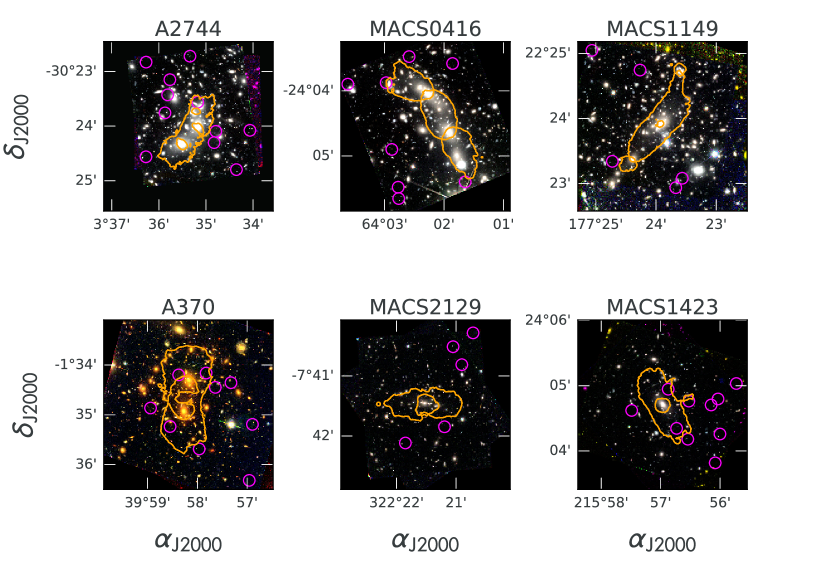
Figure 1.— 6/11 Galaxy clusters targeted in this work, including 4 Hubble Frontier Fields clusters. Critical curves (orange lines) from our lens models are shown at $z=7.6$ along with the $z\gtrsim 7$ LBGs (magenta circles) we targeted with MOSFIRE. Magnification can be as large as $\sim 50$ near the critical curve, but falls off quickly, reaching typical values of $1.5-2$ near the edge of the shown fields, which are the HST WFC3/IR footprints.

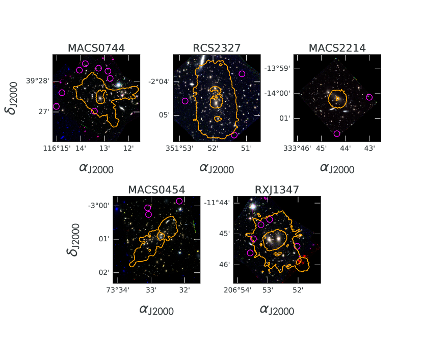
Figure 2.— Same as Figure 1, but for the remaining 5 galaxy clusters targeted in this work.

The imaging data were primarily used to measure photometric redshifts to select a sample of high-z galaxies for spectroscopic follow-up. The images were also used in constructing the lens models (Section 3.2). The data come from several HST and Spitzer/IRAC programs, summarized in Table 2. HST mosaics of the clusters used in this work are shown in Figures 1 and 2. We targeted several clusters belonging to the Hubble Frontier Fields Initiative (HFF; Lotz et al., 2016). These are Abell 2744 (A2744), M0416.1-2403 (MACS0416), MACSJ0717.5+3745 (MACS0717), MACSJ1149.5+2223 (MACS1149) and Abell 370 (A370). As explained in Section 3.1, MACS0717 had 0 targets in our final photometric selection, so it is not included in the rest of this work. For these clusters, we also use Keck/MOSFIRE $\mathrm{K_{s}}$-band photometry from the K-band Imaging of the Frontier Fields program (Brammer et al., 2016).

Another 4 clusters: MACS0744, MACS1423, MACS2129, and RXJ1347 are part of the Cluster Lensing And Supernova survey with Hubble (CLASH; Postman et al., 2012). MACS0454 was observed by HST-GO-11591/GO-9836/GO-9722, and the HST images for both MACS2214 and RCS2327 were obtained as part the Spitzer UltRa Faint SUrvey Program (SURFSUP; Bradač et al., 2014). Many of these clusters were observed by the Grism Lens-Amplified Survey from Space (GLASS; Schmidt et al., 2014; Treu et al., 2015; Schmidt et al., 2016), which obtained HST WFC3/IR imaging and grism spectroscopy of the prime cluster fields. Our target selection was mildly influenced by the Ly$\alpha$ candidates assembled by Schmidt et al. (2016, see Section 3.1).

The depths of the HST images vary among the clusters. For example, the images of the HFF clusters that we targeted all reach limiting magnitudes of $\sim 29$ AB mag ($5\sigma$, point source) per band, whereas the remaining clusters are $\sim 2$ magnitudes shallower per band. The images of the HFF and CLASH clusters were obtained from the latest public mosaics available on the Mikulski Archive for Space Telescopes (MAST^,). The HFF data span 3 Advanced Camera for Surveys (ACS) filters: F435W, F606W and F814W, and 4 Wide Field Camera 3 (WFC3) IR filters: F105W, F125W, F140W and F160W. The CLASH clusters share these filters but have 5 additional filters that we use: F475W, F625W, F775W, F850LP (ACS) and F110W (WFC3). The three non-CLASH and non-HFF clusters: MACS0454, MACS2214 and RCS2327 were processed as described by Huang et al. (2016b) and have a subset of the CLASH filters.

We also use deep Spitzer/IRAC data in tandem with the HST data. The primary purposes of these data are to more accurately select and characterize the high-$z$ sample (e.g. Huang et al., 2016b, Strait et al. 2019, in prep.). The IRAC images were obtained by the Spitzer Ultra-Faint Survey Program (SURFSUP; PID 90009; Bradač et al., 2014) and the Spitzer Frontier Fields (SFF; PIDs: 83, 137, 10171, 40652, 60034, 80168, 90257, 90258, 90259, 90260). The data have similar depths in all 12 clusters, reaching at least $\sim 30~{}\mathrm{hr}$ in the $[3.6]~{}\mu m$ and $[4.5]~{}\mu m$ bands (hereafter $[3.6]$ and $[4.5]$). The processing of the Spitzer/IRAC data is described by Ryan et al. (2014) and Huang et al. (2016b).

2.3. HST and IRAC photometry

While the HST photometry procedure is described in detail by Huang et al. (2016b), we briefly outline the primary steps we take to produce photometric catalogs. First, we produce point-spread function (PSF) matched HST images with a 60mas pixel size, convolving all images (except F160W) to match the resolution of F160W, the lowest resolution HST image. We produce a stacked near-infrared (NIR) image from the HST WFC3 images to use for object detection. We then run Source Extractor (SExtractor; Bertin & Arnouts, 1996) in dual-image mode on each filter using the stacked WFC3 NIR image as the detection image. We correct each filter for galactic extiction using the IR dust maps obtained by Schlegel et al. (1998) and the coefficients in each filter from Postman et al. (2012). We also find from simulations that the flux errors in each filter reported by SExtractor are underestimated. We correct the errors via source simulations using a similar method to Trenti et al. (2011).

For some of the clusters, i.e. the HFF clusters, MACS1423, MACS2129 and RXJ1347, we also performed a subtraction of the intra-cluster light (ICL) and bright cluster members using the method developed by the ASTRODEEP collaboration (Merlin et al., 2016; Castellano et al., 2016). This was done to obtain more accurate photometry and to improve number counts of lensed, high-redshift sources. It is important to perform on the deeper images, e.g. the HFF images, due to the stronger contamination from the ICL. However, the ICL is less of an issue for the CLASH-depth clusters, so the fact that this is was not performed on MACS0454, MACS0744, and RCS2327 is therefore of little concern. In particular, the sources that would be unveiled in these clusters from ICL and cluster member subtraction would be far too contaminated in the MOSFIRE slits to obtain constraining Ly$\alpha$ flux limits.

The IRAC photometry is described by Huang et al. (2016b). In brief, we use T-PHOT (Merlin et al., 2015) to measure colors between HST and IRAC. We use priors based on the segmentation map from the HST F160W image, the image closest in wavelength to the IRAC bands, to deblend objects in the lower resolution IRAC bands. In this way, we can assemble a consistent photometric catalog with IRAC for all of the sources identified in the HST NIR detection image. The end result of the process is a merged HST and IRAC photometric catalog for all detected sources in the field.

3. Results

3.1. Selection of high-$z$ sample

The selection criteria for including high redshift galaxies on our slit-masks was very inclusive. Where possible, we incorporated multiple selections from the literature to maximize the number of high-$z$ targets on the mask, using the compilation by Schmidt et al. (2016). Since our observations began in December 2013, we have obtained significantly improved HST and Spitzer data for many of the clusters in this sample. In particular the HFF program and much of the SURFSUP and GLASS programs were performed during this time.

In order to use a more consistent photometric selection across all clusters in this work and to make use of the much deeper current data, we performed the same photometric processing of all of the clusters in our sample after all of our spectroscopic observations were taken. We recalculated the photometry for each cluster using the pipeline described in Section 2.3 and re-fit all of the photometry to obtain photometric redshift probability distributions, $P(z)$s, and SEDs using EA$z$Y (Brammer et al., 2008), adopting the default v1.3 EA$z$Y spectral templates. As in Huang et al. (2016b), we inspected the distribution of best-fit photo-$z$s for all clusters, ensuring that the distribution peaked at the cluster redshift. For the clusters in the GLASS sample (c.f. Table 2), we were able to anchor the EA$z$Y photo-$z$ distribution by comparing our photo-$z$s to spectroscopic redshifts of intermediate-$z$ galaxies in the GLASS data set. We found good statistical agreement in all clusters (e.g. Hoag et al., 2016; Wang et al., 2015). This was not possible for the non-GLASS clusters: MACS0454, MACS2214 and RCS2327. The objects in these clusters hold less weight in the neutral fraction inference because they generally have fewer objects and shallower observations. Nonetheless, their photo-$z$s are potentially less reliable than the photo-$z$s of targets in the GLASS clusters.

We used a flat prior on $z$, rather than adopting the default magnitude prior when deriving the $P(z)$s of all objects with EA$z$Y. We did not adopt the default EA$z$Y magnitude prior because our targets are lensed. From the $P(z)$ of each galaxy we calculated the probability that Ly$\alpha$ falls in the MOSFIRE Y-band, i.e. $P(7<z<8.2)$. We then selected objects with $P(7<z<8.2)>0.01$, finding a total of 2828 such objects in all 11 clusters. A significant fraction of these were spurious. We cleaned the catalog of objects that were obvious parts of larger galaxies, diffraction spikes, bad pixels, or clearly originated from the edge effects at the boundary of the detector or overlap between epochs. This inspection was performed visually, so it is naturally subjective. However, it is more reliable than our current automatic methods to remove such artifacts. After cleaning the sample, we arrived at a sample of 530 objects that fulfill the $P(7<z<8.2)>0.01$ condition. Of these, we observed 70 in our Keck/MOSFIRE survey. 2 of these objects were spectroscopically confirmed to be at lower redshift ($6<z<7$) by Huang et al. (2016a) and S. Fuller et al. (in preparation) with Keck/DEIMOS during a simultaneous spectroscopic campaign. We note that the spectroscopic redshifts of both galaxies are consistent with the photometric redshifts we obtained for those objects with EA$z$Y. The remaining 68 objects will hereafter be referred to as the “MOSFIRE” sample. We note that while we observed several candidates from our original photometric catalogs in MACS0717 in December 2013 based on pre-HFF HST and Spitzer/IRAC imaging, the final photometric selection from our full-depth images yielded 0 candidates. As a result, MACS0717 is not part of the MOSFIRE sample, and is not discussed in the rest of this work.

During some of our observing runs, we preferentially targeted GLASS Ly$\alpha$ emitter candidates from Schmidt et al. (2016). While these represented typically only 1-2 targets per cluster, we checked that this selection did not introduce a bias into our final result. We ran the neutral fraction inference (described in Section 3.7) with and without these targets and found that the difference was insignificant. We also compared the distributions of properties of the MOSFIRE sample with the parent photometric sample. Figure 3 shows the comparison for the F160W apparent magnitude, peak photometric redshift ($z_{\mathrm{peak}}$), intrinsic absolute magnitude corrected for lensing ($M_{UV}-2.5\log_{10}(\mu/\mu_{\mathrm{best}})$), and the rest-frame UV color (measured near-IR color F125W-F160W). We performed a two-sample Kolmogorov-Smirov (KS) test for each of these properties, finding significant differences ($>99\%$ probability) between the distributions for the F160W magnitude, $z_{\mathrm{peak}}$, and the absolute magnitude. These differences illustrate our mask design strategy which was to put brighter candidates that had a higher probability of being high redshift on the masks. We correct for these selection effects when inferring the neutral fraction (see Section 3.7). The rest-UV color is statistically consistent between the two samples, which is important because we do not correct for any influence this color can have on the Ly$\alpha$ properties, such as the EW distribution.

We plot the $P(z)$s for all 68 galaxies in the MOSFIRE sample in Figure 4. Most of the probability from the 68 galaxies falls within the MOSFIRE Y-band coverage. We account for the photometric redshift impurity in the neutral fraction inference, as explained in Section 3.7. We list the targets along with some of their properties in Table A1. Throughout this work, we refer to individual targets via their cluster and ID in the following manner: the first target in Table A1 is ID=A370-000 and the last is ID=MACS0744-069. We note that the median absolute magnitude of our sample is $M_{UV}=-18.25$, where we account for magnification for each galaxy before computing the median. This is $\sim 0.1L_{\star}$ at $z\sim 7-8$ (Bouwens et al., 2015b), illustrating that the galaxies we are targeting are intrinsically very faint and probably more characteristic of the general galaxy population than $\sim L_{\star}$ galaxies.

3.2. Gravitational Lens Models

To link the observed LBGs to halos in reionization simulations for performing the inference on the hydrogen neutral fraction (see Section 3.7), we use the galaxy intrinsic luminosity. Because we observed LBGs in lensed fields, we must correct their observed luminosities by the magnification factor. To obtain the magnification factor for each galaxy, we produce lens models of all of the clusters in our sample. Lens modeling is performed using the free-from code developed by Bradač et al. (2005, 2009). Briefly, the code solves for the gravitational potential on an adaptive pixel grid via $\chi^{2}$ minimization. The lensing quantities such as convergence, shear and magnification are all derived from the best-fit gravitational potential.

The lens models for all clusters were constructed using the HST imaging data described in Section 2.2. HST images are used to identify strongly lensed (multiply-imaged) galaxies as well as weakly-lensed (singly-imaged) galaxies, both of which are used as constraints to the lens model. We also used spectroscopic redshifts from GLASS (Schmidt et al., 2014; Wang et al., 2015; Treu et al., 2016; Hoag et al., 2016), from the CLASH-VLT program (P.I.: P. Rosati; Rosati et al., 2014), and from Limousin et al. (2012); Johnson et al. (2014); Zitrin et al. (2015); Grillo et al. (2016); Monna et al. (2017); Lagattuta et al. (2017) to improve the precision of the lens models. In general, we used only the set of mulitply-imaged systems with either secure spectroscopic redshifts or consistent photometric redshifts (as in e.g. Hoag et al., 2016). To obtain uncertainties on the lensing quantities, including the magnification, we bootstrap resample the weak lensing catalog and re-run the lens modeling code 100 times. The number of weakly-lensed galaxies (typically $\sim 500-1000$) is much larger than the number of strongly-lensed galaxies, so we opt to use the weak lensing catalog for the bootstraps. In cases where the number of multiply-imaged systems is sufficiently large ($\gtrsim 15$), we simultaneously resample from the strongly-lensed and weakly-lensed galaxy catalogs to obtain uncertainties. For more details on this procedure see Hoag et al. (2016).

Some of the lens models used in this work are described in previous works: the RCS2327 model was obtained by Hoag et al. (2015), A2744 by Wang et al. (2015); MACS0416 by Hoag et al. (2016), MACS2129 by Huang et al. (2016a); MACS1423 by Hoag et al. (2017), MACS1149 by Finney et al. (2018), and A370 by Strait et al. (2018). Lens models for MACS0454, MACS0744, MACS2214 and RXJ1347 are presented here for the first time. We show the critical curves from all of our lens models as well as the location of the high redshift objects targeted in the MOSFIRE campaign with non-zero probability of being at $7<z<8.2$ in Figures 1 and 2.

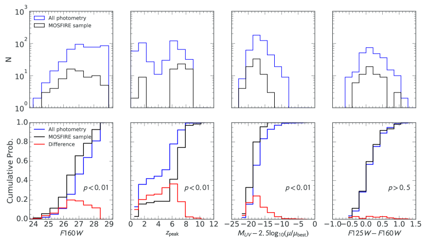
Figure 3.— Comparison of the sample targeted with MOSFIRE and the parent photometric catalog of high-$z$ sources. Top: from left to right: distributions of the HST F160W apparent magnitude, peak photometric redshift ($z_{\mathrm{peak}}$), absolute magnitude (corrected for lensing magnification) and F125W-F160W color (rest frame UV color) for the entire photometric high-$z$ sample (blue) and the MOSFIRE sub-sample. Bottom: The cumulative probability distributions of the above quantities, following the same color scheme. The red line in each panel is the difference between the two cumulative distributions, used in a two-sample Kolmogorov-Smirnov (KS) test. The KS tests indicate that the MOSFIRE sample is statistically brighter (both apparently and intrinsically) and higher redshift than the parent photometry sample. We describe how we account for these effects in Section 3.7. The distributions of rest-frame UV colors (observed IR colors: F125W - F160W) are statistically consistent between the two samples. P-values are shown in the bottom panels indicating the significance of the rejection or acceptance of the null hypothesis, i.e. that the two samples are drawn from identical distributions.

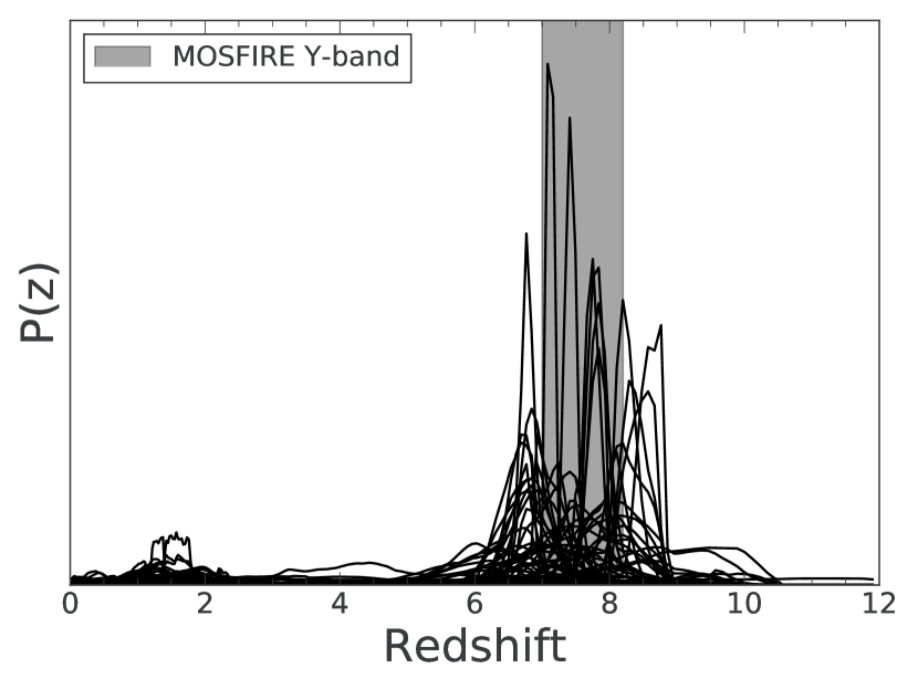
Figure 4.— Photometric redshift distributions for all 68 galaxies in the MOSFIRE sample. The light gray band denotes the MOSFIRE Y-band redshift coverage of the Ly$\alpha$ emission line, $7<z<8.2$. We account for the fact that not all of the probability distribution falls within the Y-band coverage redshift when inferring the neutral fraction (Section 3.7).

3.3. Search for Ly$\alpha$ emission

After collecting all of our MOSFIRE observations and selecting the 68 targets that fulfill our high-$z$ selection criteria, we performed an automatic search for emission lines. For each target, we calculated $S/N_{int}$, the integrated $S/N$, at each wavelength in the full-depth 1D $S/N$ spectrum, assembling the integrated signal-to-noise spectrum. We used a spectral bandpass of $6$Å ($\sim 6$ pixels) for the integration because this is twice the FWHM spectral resolution of the instrument. For each object, we flagged any wavelengths where $S/N_{int}\geq 5$, i.e. lines with high confidence. This resulted in a total of 22 candidate emission lines.

We visually inspected all 22 candidate lines identified by the automatic detection procedure. Real emission lines have several characteristics which can distinguish them from spurious features. These are:

1. Two negative residuals at symmetric positions flanking the central emission line and with approximately half of the intensity of the central emission line due to our ABBA dither pattern

2. At least as spectrally extended as the MOSFIRE resolution, i.e. $\sim 3$ pixels in Y-band

3. At least as spatially extended as the atmospheric seeing at the time of observation

4. Distinguishable from sky emission line features

Because these tests were performed visually, they are inherently subjective. However, the candidate list was short (22 candidates) and most of the candidates failed multiple of these tests obviously. There was 1 ambiguous case which we describe in Section 3.4.

3.4. Ly$\alpha$ detections

We identified 2 emission lines that passed the tests described in Section 3.3. The $S/N$ spectra for these two objects, MACS0744-064 and RXJ1347-018, are shown in Figures 5 and  6.

We observed MACS0744-064 (Figure 5) on 2016 Feb 22, 2016 Feb 23 and 2016 Mar 20 with slit-masks MACS0744_M, MACS0744_M, and MACS0744_ATH4Yband_mt_M, respectively (see Table 1). The emission line is significantly detected on 2016 Feb 23 and 2016 Mar 20, but hardly detected on 2016 Feb 22. While the exposure time was comparable for 2016 Feb 22 and 2016 Feb 23, the seeing was much worse on 2016 Feb 22, explaining the difference in $S/N$. The seeing and attenuation were both good on 2016 Feb 22 and 2016 Mar 20, the two dates where the emission line is significantly detected. ID=MACS0744-064 is confidently detected, with an integrated signal-to-noise ratio of $S/N_{int}=10.3$ in the full-depth stack. The two negative residuals are also clearly detected in the stack at the correct locations and can also be seen on multiple nights of observation. The line is completely separated from sky emission lines. As a result, this line is considered secure.

ID=RXJ1347-018 is detected at $S/N_{int}=5.1$. Unlike MACS0744-064, we only observed this object during a single night of observation, so we do not have multiple nights to corroborate the detection. To test the robustness of the detection, we split the data in half, re-reduced each half, and re-extracted the spectra to see if the emission line was present in both halves. We found a peak in the integrated signal to noise in both halves at the same wavelength as in the full-depth spectrum. Using the same bandpass as in the full-depth spectrum, we found values of $S/N_{int}=3.82$ and $S/N_{int}=3.11$ in the two halves, consistent with a real line of $S/N_{int}\sim 5$ in the combined dataset.

Despite this evidence in support of the line, there are other aspects of the line that are concerning. A sky emission line is present just blueward of the line-peak emission wavelength of $9924$Å. Part of the 6Å spectral bandpass used to calculate the integrated signal-to-noise falls on this sky emission line. While the noise spectrum in principle takes into account the noise from the sky emission line, the sky subtraction is imperfect and could introduce spurious features at this level of $S/N$. The negative residuals are present for this object with ratios of $-0.9\pm 0.3$ for both top and bottom residuals. These ratios should be consistent with $-0.5$ as a result of our dither pattern. However, because the central emission line is only detected at $S/N_{int}\sim 5$, the negative residuals themselves are only expected to be detected at $\left|{S/N_{int}}\right|\sim 3.5$. At such low $S/N$, the ratios of the negative residuals to the central emission are less robust, and thus this test is less reliable. For example, the proximity to the sky line could influence the deviation of these ratios via imperfect sky line subtraction. Given that these factors reduce our confidence in the emission line, we carry out the neutral fraction inference with and without this detection and compare the results in Section 3.7, finding that its inclusion or exclusion does not change our result in a statistically significant way. Future follow up of this cluster is needed to confirm or deny the validity of this emission line.

Both of the emission lines presented here are the only lines detected in the spectra of their respective targets. Here we provide additional evidence to properly identify them as Ly$\alpha$. For both objects, our main evidence in support of Ly$\alpha$ is the photometric redshift distribution, $P(z)$. We show the $P(z)$ plots for MACS0744-064 and RXJ1347-018 in Figures 7 and  8, respectively. In both cases, the spectroscopic redshift is in good agreement of the photometric $P(z)$, falling within the $68\%$ confidence interval. The most common contaminant of Ly$\alpha$ at $z\sim 7$ is the [O ii]$\lambda\lambda 3726,3729$ doublet at $z\sim 1.5$. The $P(z)$s suggest that [O ii] is very unlikely for both MACS0744-064 and RXJ1347-018. Furthermore, the [O ii] doublet would be resolved given the MOSFIRE resolution, with a peak separation of $\sim 7$Å. We do not detect any doublets with this separation in our spectra. Within the $95\%$ confidence interval of the $P(z)$s of both targets, the C iv and C iii] doublets could fall in MOSFIRE Y-band. However, these lines are typically much weaker in LBGs than the rest-frame equivalent widths that would be required to detect them given the faintness of these targets (e.g. Shapley et al., 2003; Stark et al., 2014; Le Fèvre et al., 2017). Furthermore, in some cases we would expect to see both lines in the doublet. However, we cannot completely rule out that high equivalent width C iv or C iii], such as values observed by Stark et al. (2015, 2016), could explain the emission lines.

The RXJ1347 emission line looks marginally double peaked, but the separation of these two features is $\sim 4$Å and cannot be explained by any strong emission line doublets at redshifts consistent with the $P(z)$. The bluer peak falls on a narrow feature in the noise spectrum in between a bright sky line and the center of the emission line, but which is not associated with the sky line. The feature originates from two pixels in the 2D noise spectrum, which are identified by the DRP. We tested to see whether this feature was responsible for the bluer bump in $S/N$ spectrum. We masked out these two pixels and re-extracted the $S/N$ spectrum, finding that the bump did not disappear, and that the integrated $S/N$ was slightly larger than in the original case. We conclude that the blue bump originates from the flux spectrum, but it could be a result of imperfect sky subtraction of the bright sky line at $\sim 9917$Å.

3.5. Physical characteristics of MACS0744-064 and RXJ1347-018

We also show the spectral energy distributions (SEDs) of both galaxies in Figures 7 and  8. We perform SED-fitting using the method described by Huang et al. (2016b). In brief, we use EA$z$Y with the Bruzual & Charlot (2003) stellar population synthesis models, adopting a Chabrier (2003) initial mass function between $0.1$ and $100M_{\odot}$, a Calzetti et al. (2000) dust attenuation law, and an exponentially declining star-formation history with a fixed metallicity of $Z=0.2Z_{\odot}$. Nebular emission lines are added to the templates as described by Huang et al. (2016b).

We find that MACS0744-064 has a considerably bluer rest-frame UV slope than RXJ1347-018. This results in a stark difference in some of their physical properties, which are provided in Tables 3 and 4. In particular, MACS0744-064 is significantly younger (age = $17.38^{+5.53}_{-6.91}~{}\mathrm{Myr}$) than RXJ1347-018 (age = $640.47^{+78.15}_{-131.73}~{}\mathrm{Myr}$). Younger stellar ages ($\sim 10-100~{}\mathrm{Myr}$) are expected at $z\sim 7$ given the relatively brief amount of time at this redshift for star-formation to have taken place since the Big Bang ($\sim 750~{}\mathrm{Myr}$). With this in mind, RXJ1347-018 is surprisingly old. However, relatively evolved stellar populations have possibly been observed at similar redshifts and beyond (e.g. Richard et al., 2011; Zheng et al., 2012; Bradač et al., 2014; Hashimoto et al., 2018, Strait et al. 2019, in prep.), suggesting the onset of star formation within the first $\sim 300~{}\mathrm{Myr}$ after the Big Bang. Katz et al. (2018) showed that the SEDs of these rare, evolved stellar populations can be reproduced by cosmological simulations, but only in the most massive halos in their simulation.

The red UV slope of RXJ1347-018 is partially driven by the detections in the IRAC $[3.6]~{}\mu m$ and $[4.5]~{}\mu m$ bands. For example, in Figure 8 we show our best-fit SED for RXJ1347-018 using only the HST constraints. The UV slope is bluer then when we include the IRAC constraints. The IRAC detections are questionable due to the presence of a bright neighboring galaxy. In Figure 9, we show a cutout of the HST F160W image as well as the two IRAC bands centered on RXJ1347-018. The galaxy is resolved in HST, but it is heavily blended with the neighboring galaxy in IRAC due to the much larger PSF. While we attempted to subtract the neighbor using T-PHOT when performing photometry on RXJ1347-018, the proximity to RXJ1347-018 makes the fluxes untrustworthy. As a result, we show the SED with and without the IRAC constraints in Figure 8, and we report the physical properties of the galaxy in both cases in Table 4. Using HST photometry only, the age of the galaxy is very poorly constrained (age = $321.00^{+397.62}_{-310.52}~{}\mathrm{Myr}$) and the stellar mass is an order of magnitude smaller than when we include the IRAC constraints.

In some cases, age and stellar mass inferences can be biased due to strong unmodeled rest-frame UV and optical emission lines falling in the near-IR HST and mid-IR IRAC filters (e.g. Schaerer & de Barros, 2009; Labbé et al., 2013; Smit et al., 2014). The strongest of such emission lines are the [O ii], [O iii], H$\beta$ and H$\alpha$ lines. At the redshift of RXJ1347-018, $z=7.161$, none of these strong lines fall in $[3.6]$, so they could not explain the bright flux in this filter even if it were real. While H$\beta$ and [O iii] fall in the $[4.5]$ band at $z=7.161$ and could potentially explain this flux, this would not explain the flux in the $[3.6]$ band.

Molino et al. (2017) performed photometry and SED-fitting for the CLASH clusters, which include MACS0744 and RXJ1347. Both MACS0744-064 and RXJ1347-018 are present in their publicly available photometric catalogs. We compare to the only two fitted quantities present in their catalog, which are the photo-$z$ and the stellar mass. For RXJ1347-018 (CLASHID$=0911$), they obtained a best-fit photometric redshift of $z=7.61^{+0.13}_{-0.81}$ (95% conf.), in agreement with the Ly$\alpha$ spectroscopic redshift (and the photo-$z$) that we measured. They report a stellar mass for RXJ1347-018 (uncertainties are not provided) of: $3.89\times 10^{9}M_{\odot}$ before accounting for magnification. Adopting our measurement of $\mu_{best}=21.4$, this results in a stellar mass of $1.82\times 10^{8}M_{\odot}$. We note that Molino et al. (2017) did not use Spitzer/IRAC data, so comparing to our stellar mass measurement of $M_{\star}=1.45^{+4.14}_{-1.19}M_{\odot}$ derived without IRAC, the two results are in agreement.

For MACS0744-064 (CLASHID$=1176$), the catalog photometric redshift is: $z=4.14^{+1.42}_{-3.70}$ (95% conf.). This is significantly different than our photo-$z$, which does not show any probability near the peak of their distribution, i.e. at $z\sim 4$ (Figure 7). We investigated different origins for this discrepancy. As for RXJ1347-018, Molino et al. (2017) do not use the IRAC $[3.6]$ and $[4.5]$ measurements as constraints on the photo-$z$. However, this is not the primary reason for the photo-$z$ discrepancy. We re-ran EA$z$Y on our photometry without the two IRAC bands, and found approximately the same photo-$z$ as when we included the IRAC data. We also checked to see if the different photo-$z$s arose due to differences in HST photometry. We re-ran EA$z$Y using the Molino et al. (2017) photometry and found $z=6.39^{+0.51}_{-5.27}$, similar to the result using our own photometry. This means that the difference most likely arises from the different codes used to derive the redshifts, rather than the photometry. Molino et al. (2017) use Bayesian photometric redshifts (BPZ; Benítez, 2000; Coe et al., 2006), whereas we use EA$z$Y. We note that the brightness of this galaxy is near the detection limit of the HST images; the $S/N$ in the four bands in which it is detected above $S/N=3$ are F160W: 3.8, F140W: 4.0, F125W: 3.4, F110W: 5.3. RXJ1347-018 is detected with much higher $S/N$ in HST, and there the photo-$z$s are in much better agreement. As a result, we expect that the different templates and other slight implementation differences between the two codes are amplified when the signal to noise ratio of the data is low, giving rise to the different photometric redshift result.

The Ly$\alpha$ properties of the two galaxies are also shown in Tables 3 and 4. We calculated rest-frame Ly$\alpha$ equivalent widths ($\mathrm{EW_{Ly\alpha}}$) by dividing the line flux by the continuum flux density measured in F160W and then by the scale factor ($1+z$). MACS0744-064 has $\mathrm{EW_{Ly\alpha}}=59.4$ Å, and RXJ1347-018 has $\mathrm{EW_{Ly\alpha}}=27.8$ Å. These are within the range of values for $\mathrm{EW_{Ly\alpha}}$ among the other known Ly$\alpha$ emitters at $z=7-7.5$ (see Table 2 of Stark et al., 2016). However, our measurements are for much fainter galaxies than are typically observed at $z\sim 7$ due to the lensing magnification. MACS0744-064 and RXJ1347-018 have intrinsic absolute magnitudes of $M_{UV}-2.5\log_{10}(\mu/\mu_{\mathrm{best}})=-18.5\pm 0.4$ mag ($L=0.12^{+0.06}_{-0.04}L_{\star}$) and $M_{UV}-2.5\log_{10}(\mu/\mu_{\mathrm{best}})=-17.2\pm 0.2$ mag ($L=0.03\pm 0.01L_{\star}$), respectively. Galaxies this faint far outnumber those observed in the field at luminosities of $L\sim L_{\star}$, which likely live in rare and massive halos (Roberts-Borsani et al., 2016; Mason et al., 2018b). As a result, we can probe the neutral hydrogen fraction from more typical halo masses at $z\sim 7-8$, as opposed to fewer halos at the high mass end. An ideal approach, and one we hope to adopt in future work, is to combine data sets to probe the neutral fraction using the entire available range of halo masses.

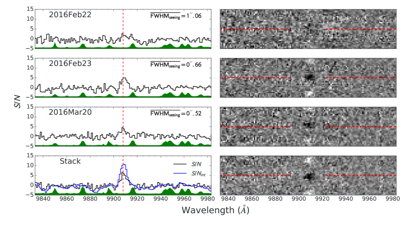
Figure 5.— Detection of Ly$\alpha$ at $9908$Å ($z_{Ly\alpha}=7.148\pm 0.001$) from ID=MACS0744-064. Left: 1D $S/N$ spectra (black histograms) from three different nights of observation and the stack of all three. The integrated $S/N$ is also shown (blue histogram) in the stacked panel, reaching $S/N_{int}=10.3$ at the line center. The vertical red dashed line in each panel is centered at $9908$Å. An arbitrarily scaled noise spectrum is shown in green in each panel. Right: 2D $S/N$ spectra from which the 1D spectra shown on the left are extracted. The red horizontal dashed lines show the expected spatial position of the object in the slit. Black represents positive values, while white represents negative values. Negative residuals are clearly seen in white on either side of the central emission line in most panels. Note that the seeing was poor ($>1^{\prime\prime}$) on 2016 Feb 22 but favorable ($<0.7^{\prime\prime}$) on the other two dates, explaining the non-detection in the top panel.

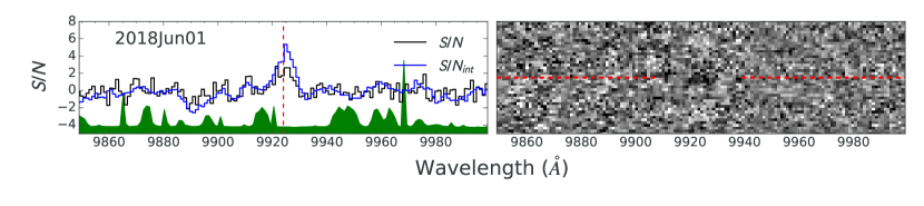
Figure 6.— Detection of Ly$\alpha$ at $9924$Å ($z_{Ly\alpha}=7.161\pm 0.001$) from sample ID=RXJ1347-018. Left: 1D $S/N$ spectrum (black histogram) from the single night of observation. The integrated $S/N$ is also shown (blue histogram) reaching $S/N_{int}=5.1$ at the line center. The vertical red dashed line is centered at $9924$Å. An arbitrarily scaled noise spectrum is shown in green. Right: 2D $S/N$ spectra from which the 1D spectra shown on the left are extracted. The red horizontal dashed lines show the expected spatial position of the object in the slit. Black represents positive values, while white represents negative values. Negative residuals are formally detected at the correct positions, although the low $S/N$ makes them hard to visually distinguish.

3.6. Non-detections

The remaining 20/22 candidate lines that were flagged by the automatic line detector are much less secure than the two lines presented above. Most fail multiple of the visual inspection tests. However, 2 of these correspond to real emission lines from a single lower-$z$ galaxy that we did not target, but which happened to fall in the same slit as one of our $z\gtrsim 7$ targets, MACS1149-014. The two emission lines are confidently identified as the [O iii]$\lambda\lambda 4959,5007$ emission line pair at $z=1.225$, and are present at a spatial offset from the central trace of our actual target consistent with that expected from the position of the slit relative to our target and the lower-$z$ contaminating galaxy in the HST image.

We note that while Hoag et al. (2017) presented a detection of Ly$\alpha$ in ID=MACS1423-040, an object in our MOSFIRE sample, it does not pass the above automatic line detection criteria. This is primarily due to our re-scaling (increasing) of the noise as described in Section 2.1. If we perform the same extraction of the line as done by Hoag et al. (2017), but use the re-scaled noise, we find $S/N_{int}=3.4$. Because the Ly$\alpha$ EW of this object is so low ($9$Å; Hoag et al., 2017), it has an insignificant impact on our neutral fraction results. We demonstrate this in section 3.7 by inferring the neutral fraction both with this target as a detection and as a non-detection.

While we likely only detect Ly$\alpha$ in 2 of the 68 galaxies in our sample, our non-detections are useful constraints on the neutral fraction. An individual $1\sigma$ flux limit spectrum, $f_{\mathrm{lim}}(\lambda)$, is obtained from the scaled noise spectrum of each object, $\sigma(\lambda)_{\mathrm{MOS,scaled}}$, via:

$$f_{\mathrm{lim}}(\lambda)=\Delta\lambda\times\sqrt{2*\mathrm{FWHM}/\Delta\lambda}\times\sigma(\lambda)_{\mathrm{MOS,scaled}},$$ (1)

where $\Delta\lambda=1.086$Å is the spectral pixel size and $\mathrm{FWHM}$ is the full-width at half maximum of the MOSFIRE Y-band spectral resolution, $\sim 3$Å. We show the median flux limit spectrum of the sample in Figure 10. An individual $1\sigma$ rest-frame Ly$\alpha$ equivalent width spectrum is obtained from the flux limit spectrum via:

$$\mathrm{EW_{Ly\alpha}}=f_{\mathrm{lim}}(\lambda)/f_{\mathrm{cont}}/(1+z)$$ (2)

where $f_{\mathrm{cont}}$ is the continuum flux density measured in F160W. We note that F160W samples the rest-UV of galaxies in our redshift range without encompassing the Ly$\alpha$ line. The neutral fraction inference uses the entire flux density spectrum in the calculation of the likelihood for each object, which takes into account the variable sensitivity of the spectrum (Mason et al. 2019, submitted).

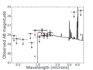
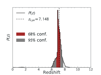
Figure 7.— Left: Best-fit Bruzual & Charlot (2003) spectral energy distribution of the target MACS0744-064 (blue) fixed at the Ly$\alpha$ redshift, $z=7.148$. Measured data points and $1\sigma$ error bars (black) and $3\sigma$ upper limits (gray) from HST and Spitzer/IRAC photometry are shown, along with the synthetic photometry from the best-fit SED (purple diamonds). Right: The photometric redshift distribution, $P(z)$ of the same galaxy obtained from EA$z$Y. The Ly$\alpha$ spectroscopic redshift is in good agreement with the photometric redshift, and there is a very small probability of a lower-$z$ solution.

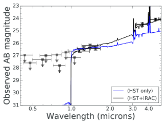
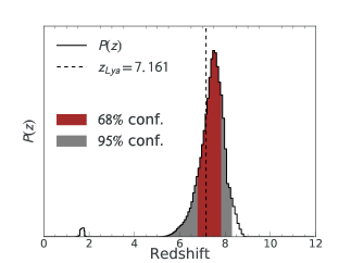
Figure 8.— Left: Best-fit Bruzual & Charlot (2003) spectral energy distribution of the target RXJ1347-018 fixed at the Ly$\alpha$ redshift of $z=7.161$. The layout is the same as in Figure 7, except that here we also show the best-fit SED using only the HST photometry in blue. The IRAC photometry is contaminated by a bright neighbor (Figure 9), so we consider the SED with and without the IRAC constraints. Right: The photometric redshift distribution, $P(z)$ of the RXJ1347-018 obtained from EA$z$Y (using the IRAC constraints). The Ly$\alpha$ spectroscopic redshift is in good agreement with the photometric redshift, and there is a very small probability of a lower-$z$ solution. This is still the case when using only the HST photometry to infer the $P(z)$.

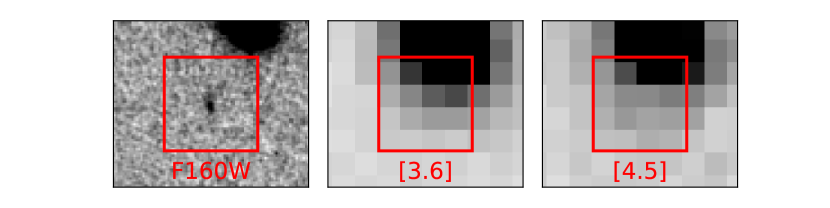
Figure 9.— HST and Spitzer/IRAC images of RXJ1347-018. Shown are the HST F160W (left), IRAC $[3.6]~{}\mu m$ (middle) and IRAC $[4.5]~{}\mu m$ images. While the galaxy is well resolved in HST, it is heavily blended with the much brighter neighbor galaxy in the two IRAC bands due to the larger PSF. As a result, the detections in the two IRAC bands are not trustworthy. The red box is $2\farcs 5$ on a side.

Table 3Properties of MACS0744-064

Quantity	Unit	Value
$\alpha_{\mathrm{J2000}}$	(degree)	116.24648
$\delta_{\mathrm{J2000}}$	(degree)	39.46042
$F160W$	mag	$27.17\pm 0.38$
$[3.6]$	mag	$<25.54$
$[4.5]$	mag	$<25.37$
$\mu_{\mathrm{best}}$		$3.2\pm 0.1$
$M_{UV}-2.5\mathrm{log}_{10}(\mu/\mu_{\mathrm{best}})$	mag	$-18.5\pm 0.4$
$L_{UV}\times\mu/\mu_{\mathrm{best}}$	$L_{\star}$	$0.12^{+0.06}_{-0.04}$
$z_{\mathrm{phot}}$		$6.9^{+0.5}_{-0.2}$
$z_{Ly\alpha}$		$7.148\pm 0.001$
$\mathrm{SFR}\times\mu/\mu_{\mathrm{best}}$	$M_{\odot}/\mathrm{yr}$	$0.66^{+0.18}_{-0.11}$
$M_{\star}\times\mu/\mu_{\mathrm{best}}$	$10^{7}M_{\odot}$	$1.11^{+0.35}_{-0.28}$
Age	$\mathrm{Myr}$	$17.38^{+5.53}_{-6.91}$
E(B-V)	mag	$<0.01$
$f_{,Ly\alpha}$	$10^{-18}\mathrm{erg\,s^{-1}\,cm^{-2}}$	$7.1\pm 0.7$
$W_{0,Ly\alpha}$	Å	$58.3\pm 25.1$
$\mathrm{FWHM_{Ly\alpha}}$	Å	$5.4\pm 1.3$
$S/N_{int,Ly\alpha}$		10.3

Note. — IRAC $[3.6]$ and $[4.5]$ magnitude limits are $3\sigma$. The factor $\mu/\mu_{\mathrm{best}}$ is introduced to show how the magnification factor enters into some properities, where $\mu_{\mathrm{best}}$ is the best-fit magnification value measured in this work. This factor allows one to re-calculate the value of a given property provided with a new magnification factor. $M_{UV}$ and $L_{UV}$ are calculated using the $F160W$ magnitude to approximate the rest-frame $UV$ luminosity. $L_{\star}$ is calculated from $M_{UV}^{\star}=20.87\pm 0.26$ measured by Bouwens et al. (2015b) at $z=6.8$.

Table 4Properties of RXJ1347-018

Quantity	Unit	Value
$\alpha_{\mathrm{J2000}}$	(degree)	206.89124
$\delta_{\mathrm{J2000}}$	(degree)	-11.75261
$F160W$	mag	$26.43\pm 0.14$
$[3.6]$	mag	$24.47\pm 0.17$
$[4.5]$	mag	$24.07\pm 0.11$
$\mu_{\mathrm{best}}$		$21.4^{+1.7}_{-1.3}$
$M_{UV}-2.5\mathrm{log}_{10}(\mu/\mu_{\mathrm{best}})$	mag	$-17.2\pm 0.2$
$L_{UV}\times\mu/\mu_{\mathrm{best}}$	$L_{\star}$	$0.03\pm 0.01$
$z_{\mathrm{phot}}$		$7.5^{+0.3}_{-0.7}$
$z_{Ly\alpha}$		$7.161\pm 0.001$
$\mathrm{SFR}\times\mu/\mu_{\mathrm{best}}$	$M_{\odot}/\mathrm{yr}$	$3.40^{+1.45}_{-0.59}$
$M_{\star}\times\mu/\mu_{\mathrm{best}}$	$10^{7}M_{\odot}$	$143.34^{+26.38}_{-35.18}$
Age	$\mathrm{Myr}$	$640.47^{+78.15}_{-131.73}$
$(\mathrm{SFR}\times\mu/\mu_{\mathrm{best}})_{\mathrm{HST}}$	$M_{\odot}/\mathrm{yr}$	$1.59^{+3.63}_{-1.05}$
$(M_{\star}\times\mu/\mu_{\mathrm{best}})_{\mathrm{HST}}$	$10^{7}M_{\odot}$	$14.53^{+41.37}_{-11.88}$
$\mathrm{(Age)_{HST}}$	$\mathrm{Myr}$	$321.00^{+397.62}_{-310.52}$
E(B-V)	mag	$<0.35$
$f_{,Ly\alpha}$	$10^{-18}\mathrm{erg\,s^{-1}\,cm^{-2}}$	$6.6\pm 1.3$
$W_{0,Ly\alpha}$	Å	$27.2\pm 6.5$
$\mathrm{FWHM_{Ly\alpha}}$	Å	$7.6\pm 1.3$
$S/N_{int,Ly\alpha}$		5.1

Note. — Quantities with subscript $\mathrm{HST}$ are derived from the best-fit SED to HST photometry only, whereas the other quantities include the IRAC photometry. The uncertainty on $\mathrm{FWHM_{Ly\alpha}}$ does not include additional uncertainty introduced due to the sky emission line blueward of the emission peak.

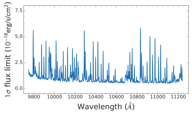
Figure 10.— Median $1\sigma$ flux limit of all 68 targets in the MOSFIRE sample. The limits shown here are calculated assuming unresolved lines using a spectral bandpass of twice the FWHM of the MOSFIRE Y-band grating. We use resolved lines when computing the likelihood on the neutral fraction for each object, which slightly decreases the sensitivity. The spikes in sensitivity at certain wavelength are due to the sky emission, and the variation is accounted for in the Bayesian framework from which we infer the neutral hydrogen fraction (Mason et al. 2019, submitted). The median flux limits vary from $\sim 1-5\times 10^{-18}\mathrm{erg/s/cm^{2}}$ among the 68 targets, assuming unresolved lines.

3.7. Neutral fraction inference

Here we use the formalism introduced by Treu et al. (2012) and extended by Mason et al. (2018a, Mason et al. 2019, submitted) including models by Mesinger et al. (2015) to infer the volume-averaged neutral hydrogen fraction in the IGM at $z\sim 7.5$ using our Ly$\alpha$ spectroscopy from MOSFIRE. We adopt $z=7.6$ as our fiducial redshift as it is the average Ly$\alpha$ redshift probed by the MOSFIRE Y-band. The formalism uses the Evolution of 21cm Structure cosmological simulations (Mesinger et al., 2015, 2016), i.e. cosmological-scale IGM simulations of inhomogeneous reionization, to obtain the global neutral fraction distribution as well as a realistic treatment of the impact of the ISM and CGM on the emerging Ly$\alpha$ line.

The model yields a likelihood that can be used to interpret observables of LBGs in terms of neutral fraction. The input observables are the rest-frame Ly$\alpha$ equivalent width measurements and limits (for non-detections) as well as galaxy luminosities. For non-detections, we use the entire flux density and noise spectra, taking into account the varying sensitivity as a function of wavelength (see Figure 10).

Our ignorance of the underlying Ly$\alpha$ FWHM distribution of the objects without Ly$\alpha$ detections introduces uncertainty into the inferred neutral fraction. Furthermore, larger assumed FWHMs result in weaker constraints due to the line flux being spread out over more detector pixels. To parameterize our ignorance on the FWHM, we marginalize over it when calculating the posterior for each object. We explored three different priors for the FWHM distribution: 1) A uniform prior between $100-400~{}\mathrm{km/s}$ for each object, 2) a log-normal $p(\mathrm{FWHM}|M_{UV})$ that uses the Mason et al. (2018a) scaling relation between Ly$\alpha$ velocity offset and $M_{UV}$ and the Verhamme et al. (2018) scaling relation between velocity offset and FWHM, where we adopt the median $M_{UV}$ of the sample for each object, 3) the same functional form and scaling relations as in (2), but where we use the individual $M_{UV}$ for each galaxy rather than the median of the sample in the scaling relations. We found that the result was robust against the choice of prior, so we adopted case (3) as it is the most physically motivated. The log-normal tends to peak around $50-100~{}\mathrm{km/s}$ for the $M_{UV}$ values in the MOSFIRE sample. For more details and the form of the full likelihood, see Mason et al. (2018a).

We also use the photometric redshift probability distributions $P(z)$ as priors in the likelihood. Effectively, we weight each galaxy in the inference, where the weight applied is given by the probability that Ly$\alpha$ falls within the MOSFIRE Y-band, i.e. $P(7<z<8.2)$. Doing so accounts for the photometric redshift impurity of our sample. Galaxy intrinsic luminosities enter into the inference via the halo-mass dependence (and hence luminosity dependence) of the local neutral fraction in the IGM simulations. Furthermore, the model assumes an intrinsic emitted EW distribution at $z\sim 6$ before any attenuation. This model is based off of real observations at $z\sim 6$ compiled by De Barros et al. (2017). For more details see Mason et al. (2018a) and Mason et al. (2019, submitted).

After applying the prior, we obtain the posterior, $p(\overline{x}_{\mathrm{HI}}|\{\mathrm{f}(\lambda),m,\mu\}$) where the data consist of the set of flux density spectra, $\mathrm{f}(\lambda)$, apparent magnitudes, $m$, and magnifications, $\mu$. For objects where there are detections, we use the measured equivalent width of the line rather than the entire flux spectrum to construct the posterior.

We show our posterior on the volume-averaged neutral fraction $\overline{x}_{\mathrm{HI}}$ in Figure 11. Using our fiducial sample of 2 Ly$\alpha$ detections (see Section 3.3), we infer a neutral fraction of $\overline{x}_{\mathrm{HI}}=0.88^{+0.05}_{-0.10}$. Our result is robust against the set of Ly$\alpha$ detections we choose, as long as the MACS0744-064 detection is included. Excluding the RXJ1347-018 detection (the 1 detection case), we infer a statistically consistent neutral fraction to the fiducial case: $\overline{x}_{\mathrm{HI}}=0.89^{+0.04}_{-0.10}$. If instead we include the additional Ly$\alpha$ detection presented by Hoag et al. (2017) (the 3 detection case), we also infer a statistically consistent neutral fraction: $\overline{x}_{\mathrm{HI}}=0.88^{+0.05}_{-0.09}$. The difference between the three cases shown is small because in all cases the MACS0744-064 detection is included. This detection is $S/N\sim 10$, so it has much larger statistical weight in the inference than the other detections. While we find the 0 detection case unlikely, we cannot rule it out because there is a small chance that the single emission line in each of the three spectra is not Ly$\alpha$. If this were the case, we would put a lower limit on neutral fraction.

4. Discussion

Our fiducial result of $\overline{x}_{\mathrm{HI}}=0.88^{+0.05}_{-0.10}$ implies a universe at $z\sim 7.5$ that is mostly neutral. This result is the most precise constraint on $\overline{x}_{\mathrm{HI}}$ at $z\gtrsim 7$, and it is consistent with the emerging picture from other probes of reionization implying a “late” and rapid reionization scenario. In Figure 12, we show published constraints on the neutral fraction from other authors. These constraints come from various independent approaches: 1) the “dark fraction” in quasar spectra, which provide upper limits on $\overline{x}_{\mathrm{HI}}$ at $z=5.7,5.9,6.1$ (McGreer et al., 2015), 2) an upper limit from Ly$\alpha$ clustering measurements at $z=6.6$ (Ouchi et al., 2010), 3) measurements of the Ly$\alpha$ damping wings of QSOs at $z=7.08$ (Greig et al., 2017) and $z=7.54$ (Bañados et al., 2018), and 4) the same approach as in this work done by Mason et al. (2018a) at $z=6.9\pm 0.5$ and Mason et al. (2019, submitted) at $z=7.9\pm 0.6$. Specifically, Mason et al. (2018a) used Ly$\alpha$ spectroscopy of 68 LBGs at $z\sim 7$ compiled by Pentericci et al. (2014), spanning a wide range in intrinsic luminosity ($-22.75\lesssim M_{UV}\lesssim-17.8$) over multiple sight lines. Mason et al. (2019, submitted) used the KMOS IFU to target 53 lensed galaxies at $z\sim 8$, providing an excellent consistency check with our work.

The closest measurement in redshift to ours is by Bañados et al. (2018), who discovered the bright QSO ULASJ1342+0928 at $z=7.54$, inferring a neutral fraction of $\overline{x}_{\mathrm{HI}}=0.56^{+0.21}_{-0.18}$ from the quasar’s Ly$\alpha$ damping wing. Greig et al. (2018) performed an independent analysis of this object using a complementary technique and found a lower fraction: $\overline{x}_{\mathrm{HI}}=0.21^{+0.17}_{-0.19}$. Taken together, these two inferences from the same object span a large range in the neutral fraction at $z\sim 7.5$, which are lower than our neutral fraction constraint, albeit with large uncertainties. At this point, the uncertainties are large enough that the results are not in significant statistical disagreement with our result. We also point out that their measurement is derived from a single QSO, which probes only a single line of sight through the IGM.

Because the hosts of QSOs such as the ones detected by Greig et al. (2017) and Bañados et al. (2018) are probably very massive halos, one might expect them to reside in more ionized regions of the universe at $z>7$. The authors attempt to account for this bias by linking their observations to halos in a global reionization simulation, as done in this work. Similarly, Mason et al. (2018a) targeted a higher luminosity sample of galaxies, and rely on the same reionization simulations in this work to infer the global neutral fraction. We stress that using a large sample of low luminosity galaxies, as achieved in this work with gravitational lensing, allows us to sample the neutral fraction from more typical-luminosity halos directly, rather than relying on the model to extrapolate using only the rarer, massive halos. In future work, we plan to use the full range of halo masses probed by the data in a consistent manner to infer the neutral fraction.

We also compare our result to the inferences by Mason et al. (2018a) at $z\sim 7$ and Mason et al. (2019, submitted) at $z\sim 8$, who used the same framework as us to infer the neutral fraction. It is reassuring that we find a more neutral universe at $z\sim 7.5$ than their result at $z\sim 7$. Similarly, their lower limit at $z\sim 8$ of $>0.76$ ($68\%$ confidence) is consistent with our inference.

We note that the range in redshift probed by our result is large, covering $z=7-8.2$, a period over which the neutral fraction is likely rapidly evolving. In fact, both of our Ly$\alpha$ detections are at $z<7.2$, hinting at evolution within our own data set. We opted to not bin our data in redshift more finely due to the already large uncertainty in a single redshift bin. Combining our data with other similar data sets in the future may allow us to meaningfully separate the data in redshift.

In Figure 12, we show various reionization histories derived from the Mason et al. (2015) luminosity function (LF) models. The two parameters of these models that we vary are the mean Lyman-continuum escape fraction, $\langle f_{\mathrm{esc}}\rangle$, and the cut-off luminosity when extrapolating the LF. To construct these histories, we also assume a log-normal ionizing efficiency, $\xi_{\mathrm{ion}}$ with mean 25.2 and standard deviation of 0.15 dex, as well as a uniform distribution for the clumping factor over the range $C=1-6$. Estimates from our data and those from similar works exclude earlier reionization histories which require large mean escape fractions ($\langle f_{\mathrm{esc}}\rangle\gtrsim 0.2$) and faint cutoff luminosities ($M_{UV}\lesssim-12$). Such scenarios result in an earlier reionization due to a higher abundance of ionizing photons at higher redshift. The escape fraction and cutoff luminosity are somewhat degenerate from the allowed reionization histories. For example, a brighter cutoff luminosity with large $\langle f_{\mathrm{esc}}\rangle$ has a similar reionization history to one with a fainter cutoff luminosity but smaller $\langle f_{\mathrm{esc}}\rangle$. With current data, the two scenarios cannot be distinguished. In future work, we hope to constrain the allowed parameter space of $\langle f_{\mathrm{esc}}\rangle$ and cutoff luminosity using all available constraints on the neutral fraction.

The escape fraction is notoriously difficult to measure, even at lower redshift. At redshifts during reionization, ionizing radiation is efficiently absorbed by the neutral hydrogen in the IGM. The cutoff luminosity, on the other hand, will be more tightly constrained via extremely deep surveys with the James Webb Space Telescope (JWST), though the exact value is likely deeper than even JWST will probe. Currently, there is no strong evidence that the $z>6$ LF deviates from a very steep faint-end slope ($\alpha\lesssim-2$; Finkelstein et al., 2015; Livermore et al., 2017; Bouwens et al., 2017). A hopeful scenario is if the cutoff luminosity can be well-constrained by future observations and uncertainties on measurements of the neutral fraction such as the one presented here are reduced. In this case, the escape fraction could be inferred. This is one example in which constraining the neutral fraction can inform the properties of galaxies at the earliest epochs.

Our neutral fraction constraint is among only a handful at $z>7$, each with large uncertainties. To better constrain the reionization timeline, and ultimately the sources of the reionization, more constraints at $z\sim 7-8$ and constraints at higher redshifts ($z\gtrsim 8$) are needed. From the current data, it is clear that reionization is ongoing at $z\sim 7-8$, so prospects of constraining the timeline with future surveys are bright. The method adopted in this work is readily deployed with JWST at higher redshift. In particular, the NIRSPEC instrument is equipped with a multi-object spectrograph similar to MOSFIRE that is able to probe to longer wavelengths ($\sim 1-5~{}\mu m$) with higher efficiency. In analogy to the GLASS Ly$\alpha$ survey (Schmidt et al., 2016), JWST NIRISS observations will also potentially allow a more complete follow-up of clusters via sensitive grism spectroscopy due to its simultaneous full field coverage and lack of slit losses. While the number of photometric targets at $z\gtrsim 8$ per cluster is currently small ($<5$/cluster), JWST NIRCAM will find larger samples with its superior sensitivity to HST, making an analysis akin to this work at $z\gtrsim 8$ a possibility.

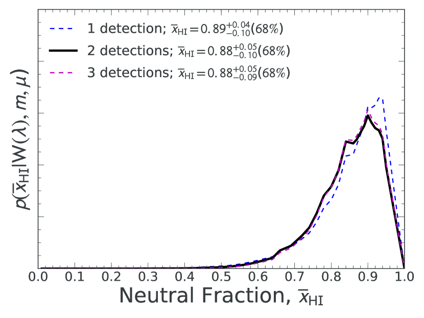
Figure 11.— Inference on the volume-averaged neutral hydrogen fraction, $\overline{x}_{\mathrm{HI}}$, at $z=7.6\pm 0.6$ using the MOSFIRE sample of 68 galaxies. We infer a neutral fraction of $\overline{x}_{\mathrm{HI}}=0.88^{+0.05}_{-0.10}$ in our fiducial case (2/68 Ly$\alpha$ detections; solid black). We show the posterior distributions for the neutral fraction for 2 other scenarios (see Section 3.3): 1/68 Ly$\alpha$ detection (blue dashed), and 3/68 Ly$\alpha$ detections (magenta dashed). All cases have one detected object in common: MACS0744-064, the Ly$\alpha$ detection in which we are most confident ($S/N_{int}\sim 10$). The fact that the difference between the scenarios is very small illustrates the influence that MACS0744-064 has on the inference, and the unimportance of low $S/N$ detections.

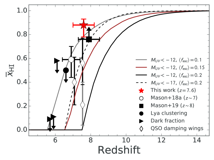
Figure 12.— Constraints on the volume-averaged neutral hydrogen fraction, $\overline{x}_{\mathrm{HI}}$, during reionization, including our constraint at $z=7.6$ of $\overline{x}_{\mathrm{HI}}=0.88^{+0.05}_{-0.10}$ (red star). The four curves correspond to different reionization histories derived from the Mason et al. (2015) luminosity function (LF) models. The two parameters of these models are the mean Lyman-continuum escape fraction, $\langle f_{\mathrm{esc}}\rangle$, and the faint-end cut-off luminosity when extrapolating the LF. The data collectively exclude reionization histories with both large mean escape fractions ($\langle f_{\mathrm{esc}}\rangle\gtrsim 0.2$ with faint cutoff luminosities $M_{UV}\lesssim-12$, which would result in an earlier reionization. The QSO damping wing measurement of $\overline{x}_{\mathrm{HI}}=0.56^{+0.21}_{-0.18}$ at $z=7.54$ by Bañados et al. (2018) (black open diamond) and the re-measurement from the same QSO by Greig et al. (2018) (gray open diamond) are both shown.

5. Summary

We presented a spectroscopic campaign targeting lensed LBGs in 12 galaxy cluster fields using Keck MOSFIRE. Using a consistent photometric selection across the 12 fields, we obtained a sample of 70 LBGs. 2 of these were confirmed to be at $6<z<7$ by a different spectroscopic campaign running simultaneously with our campaign, so we do not include those in our inference on the neutral fraction. Among the remaining 68 targets, we identified 2 probable Ly$\alpha$ emitters, one at $z=7.148\pm 0.001$ in MACS0744 and the other at $7.161\pm 0.001$ in RXJ1347. Both Ly$\alpha$ emitters are faint ($M_{UV}=-18.5\pm 0.4$ and $M_{UV}=-17.2\pm 0.2$, respectively). We also obtained sensitive Ly$\alpha$ flux and equivalent width limits for the targets from which we did not detect Ly$\alpha$.

We used the Bayesian framework of Mason et al. (2018a, Mason et al. 2019, submitted) to infer the volume-averaged neutral hydrogen fraction, $\overline{x}_{\mathrm{HI}}$, from our Ly$\alpha$ spectroscopy, taking into account the luminosity of each galaxy when linking to simulated halos in a realistic large-scale reionization simulation. We inferred a neutral hydrogen fraction of $\overline{x}_{\mathrm{HI}}=0.88^{+0.05}_{-0.10}$ at $z=7.6\pm 0.6$. Our result favors a late reionization scenario, consistent more so with the Planck Collaboration et al. (2016b) optical depth to reionization than the higher optical depth inferred from the full-depth WMAP dataset. With larger samples on current and future telescopes, this method holds promise to precisely constrain the evolution of the hydrogen neutral fraction and ultimately the timeline of cosmic reionization.

List of spectroscopic targets

Table A1Keck/MOSFIRE spectroscopic targets

Cluster	ID	RA	DEC	$H_{160}$	$\mu$	$M_{UV}$	$z_{\mathrm{phot}}$	dates of observation	$t_{\mathrm{exp}}$	$\sigma_{\mathrm{EW}}$
		(deg.)	(deg.)	(mag.)		(mag.)		(UTC)	(s)	(Å)
A370	0	39.982354	-1.581067	$26.47\pm 0.09$	$8.3^{+0.1}_{-0.1}$	$-18.4^{+0.1}_{-0.1}$	$8.2^{+0.4}_{-0.3}$	2013Dec16/2013Dec18	6660	6.2
A370	1	39.963746	-1.569358	$26.00\pm 0.06$	$18.9^{+1.0}_{-0.7}$	$-17.9^{+0.1}_{-0.1}$	$7.8^{+0.2}_{-0.2}$	2013Dec16/2013Dec18/2017Oct01	21240	2.5
A370	2	39.960679	-1.574164	$25.57\pm 0.05$	$16.2^{+0.1}_{-0.2}$	$-18.5^{+0.1}_{-0.1}$	$7.8^{+0.1}_{-0.2}$	2013Dec16/2013Dec18	6660	2.6
A370	3	39.972946	-1.569983	$28.04\pm 0.26$	$12.5^{+0.3}_{-0.3}$	$-13.3^{+0.3}_{-0.3}$	$1.4^{+2.3}_{-1.0}$	2017Oct01	14580	9.4
A370	4	39.975808	-1.587256	$26.70\pm 0.11$	$7.2^{+0.1}_{-0.1}$	$-18.3^{+0.1}_{-0.1}$	$8.2^{+0.2}_{-6.4}$	2017Oct01	14580	3.9
A370	5	39.955425	-1.572589	$27.33\pm 0.15$	$5.2^{+0.2}_{-0.1}$	$-18.1^{+0.2}_{-0.1}$	$8.2^{+0.1}_{-6.8}$	2017Oct01	14580	5.9
A370	6	39.966071	-1.594767	$27.56\pm 0.19$	$8.6^{+1.3}_{-1.0}$	$-17.3^{+0.2}_{-0.2}$	$8.1^{+0.3}_{-0.9}$	2017Oct01	14580	7.2
A370	7	39.948246	-1.586531	$27.56\pm 0.25$	$2.3^{+0.1}_{-0.1}$	$-18.5^{+0.2}_{-0.2}$	$7.2^{+0.6}_{-5.5}$	2017Oct01	14580	7.0
A370	8	39.964604	-1.613703	$26.10\pm 0.22$	$\cdots$	$-21.6^{+0.2}_{-0.2}$	$11.3^{-2.8}_{-10.2}$	2017Oct01	14580	2.9
A370	9	39.949317	-1.605278	$24.40\pm 0.05$	$2.0^{+0.0}_{-0.0}$	$-21.8^{+0.1}_{-0.1}$	$7.1^{+0.1}_{-0.1}$	2017Oct01	14580	0.4
MACS1149	10	177.394529	22.382308	$28.35\pm 0.18$	$1.7^{+0.0}_{-0.0}$	$-18.3^{+0.2}_{-0.2}$	$8.5^{0.0}_{-7.3}$	2016Feb22	10800	32.5
MACS1149	11	177.392725	22.384714	$28.64\pm 0.28$	$1.7^{+0.0}_{-0.0}$	$-16.5^{+0.3}_{-0.3}$	$3.3^{+1.2}_{-2.5}$	2016Feb22	10800	34.9
MACS1149	12	177.412083	22.389050	$27.92\pm 0.13$	$5.6^{+0.1}_{-0.1}$	$-17.1^{+0.1}_{-0.1}$	$6.8^{+0.2}_{-0.5}$	2016Feb22	10800	18.8
MACS1149	13	177.404417	22.412400	$27.70\pm 0.12$	$2.0^{+0.0}_{-0.0}$	$-18.5^{+0.1}_{-0.1}$	$7.3^{0.0}_{-6.9}$	2016Feb22	10800	16.2
MACS1149	14	177.417746	22.417442	$25.08\pm 0.03$	$1.6^{+0.0}_{-0.0}$	$-21.5^{+0.0}_{-0.0}$	$7.8^{+0.1}_{-0.2}$	2016Feb22	10800	1.7
RXJ1347	15	206.867204	-11.756654	$27.72\pm 0.27$	$34.6^{+8.2}_{-5.7}$	$-14.6^{+0.3}_{-0.3}$	$4.4^{+1.1}_{-1.5}$	2018Jun01	11700	15.9
RXJ1347	16	206.882308	-11.742173	$27.00\pm 0.19$	$20.3^{+1.5}_{-1.1}$	$-16.6^{+0.2}_{-0.2}$	$6.8^{+0.1}_{-0.2}$	2018Jun01	11700	8.2
RXJ1347	17	206.887116	-11.745009	$25.66\pm 0.08$	$17.3^{+0.9}_{-0.8}$	$-18.1^{+0.1}_{-0.1}$	$6.7^{+0.3}_{-0.2}$	2018Jun01	11700	2.5
RXJ1347	18	206.891246	-11.752606	$26.43\pm 0.14$	$21.4^{+1.7}_{-1.3}$	$-17.3^{+0.2}_{-0.2}$	$7.5^{+0.3}_{-0.7}$	2018Jun01	11700	$\cdots$
RXJ1347	19	206.893075	-11.760237	$27.92\pm 0.34$	$15.3^{+1.0}_{-0.9}$	$-16.0^{+0.4}_{-0.3}$	$6.9^{+0.6}_{-1.8}$	2018Jun01	11700	19.4
RCS2327	20	351.852258	-2.062694	$26.61\pm 0.29$	$5.2^{+0.9}_{-0.5}$	$-18.6^{+0.3}_{-0.3}$	$7.4^{+0.4}_{-7.1}$	2013Dec15/2013Dec17/2013Dec18	10620	4.7
RCS2327	21	351.856092	-2.093228	$26.38\pm 0.27$	$15.7^{+4.1}_{-3.0}$	$-14.1^{+0.4}_{-0.4}$	$1.1^{+5.3}_{-0.1}$	2013Dec15/2013Dec17/2013Dec18	10620	3.9
RCS2327	22	351.880600	-2.076275	$24.83\pm 0.05$	$4.9^{+0.4}_{-0.3}$	$-20.5^{+0.1}_{-0.1}$	$7.4^{+0.1}_{-0.1}$	2013Dec15/2013Dec17/2013Dec18	10620	1.0
MACS2129	23	322.345250	-7.671411	$25.65\pm 0.15$	$1.5^{+0.1}_{-0.1}$	$-18.6^{+0.2}_{-0.2}$	$2.0^{+0.3}_{-1.7}$	2015May28/2015Nov07/2015Nov08	25560	1.1
MACS2129	24	322.350850	-7.675244	$26.38\pm 0.13$	$1.7^{+0.0}_{-0.0}$	$-19.9^{+0.1}_{-0.1}$	$6.5^{0.0}_{-6.0}$	2015May28/2015Nov07/2015Nov08	25560	2.2
MACS2129	25	322.348408	-7.680228	$27.17\pm 0.18$	$2.1^{+0.0}_{-0.0}$	$-15.9^{+0.2}_{-0.2}$	$1.3^{+5.2}_{-0.9}$	2015May28/2015Nov07/2015Nov08	25560	4.5
MACS2129	26	322.353242	-7.697442	$26.79\pm 0.19$	$\cdots$	$\cdots$	$\cdots$	$\cdots$	$\cdots$	$\cdots$
MACS2129	27	322.364192	-7.701939	$27.40\pm 0.28$	$2.7^{+0.2}_{-0.2}$	$-18.6^{+0.3}_{-0.3}$	$7.7^{-0.6}_{-7.1}$	2015May28/2015Nov07/2015Nov08	25560	5.5
MACS0416	28	64.030963	-24.059686	$27.68\pm 0.16$	$2.7^{+0.1}_{-0.1}$	$-15.6^{+0.2}_{-0.2}$	$1.6^{+0.1}_{-1.3}$	2015Nov07/2015Nov08	16200	8.6
MACS0416	29	64.043133	-24.057911	$28.09\pm 0.16$	$5.6^{+0.1}_{-0.1}$	$-17.4^{+0.1}_{-0.2}$	$9.5^{+0.2}_{-7.5}$	2015Nov07/2015Nov08	16200	15.1
MACS0416	30	64.049583	-24.064589	$27.56\pm 0.17$	$144.8^{+399.3}_{-73.1}$	$-14.2^{+1.4}_{-0.8}$	$8.1^{+0.4}_{-0.6}$	2015Nov07/2015Nov08	16200	8.3
MACS0416	31	64.060329	-24.064961	$28.16\pm 0.16$	$4.6^{+0.1}_{-0.1}$	$-17.4^{+0.2}_{-0.2}$	$8.1^{0.0}_{-0.9}$	2015Nov07/2015Nov08	16200	14.0
MACS0416	32	64.027421	-24.089975	$25.18\pm 0.03$	$14.9^{+8.7}_{-2.4}$	$-19.0^{+0.5}_{-0.2}$	$7.8^{0.0}_{-0.3}$	2015Nov07/2015Nov08	16200	1.0
MACS0416	33	64.047992	-24.081669	$26.76\pm 0.06$	$2.5^{+0.1}_{-0.1}$	$-19.5^{+0.1}_{-0.1}$	$8.8^{-0.1}_{-0.4}$	2015Nov07/2015Nov08	16200	4.1
MACS0416	34	64.046212	-24.091339	$28.00\pm 0.24$	$2.2^{+0.1}_{-0.0}$	$-18.4^{+0.2}_{-0.3}$	$8.7^{+0.7}_{-6.7}$	2015Nov07/2015Nov08	16200	13.5
MACS0416	35	64.046063	-24.094239	$28.03\pm 0.15$	$2.4^{+0.1}_{-0.1}$	$-17.9^{+0.2}_{-0.1}$	$6.8^{+0.3}_{-0.5}$	2015Nov07/2015Nov08	16200	11.2
MACS2214	36	333.716917	-14.002444	$26.26\pm 0.45$	$1.5^{+0.0}_{-0.0}$	$-20.5^{+0.5}_{-0.4}$	$7.9^{+0.2}_{-0.8}$	2017Oct01	14400	2.9
MACS2214	37	333.739317	-14.026907	$26.35\pm 0.33$	$1.4^{+0.1}_{-0.0}$	$-20.1^{+0.4}_{-0.3}$	$6.3^{+0.1}_{-5.3}$	2017Oct01	14400	2.6
MACS1423	38	215.958129	24.077017	$27.20\pm 0.22$	$3.0^{+0.0}_{-0.0}$	$-16.1^{+0.2}_{-0.2}$	$1.8^{+4.7}_{-0.7}$	2015May28/2016Mar20/2015Apr27	31500	4.1
MACS1423	39	215.942100	24.079403	$26.01\pm 0.13$	$1.6^{+0.1}_{-0.0}$	$-20.3^{+0.1}_{-0.1}$	$6.8^{+0.2}_{-5.6}$	2015May28/2016Mar20/2015Apr27	31500	1.5
MACS1423	40	215.942400	24.069656	$25.03\pm 0.08$	$10.0^{+1.9}_{-1.8}$	$-19.7^{+0.2}_{-0.2}$	$8.3^{+0.3}_{-0.2}$	2015May28/2016Mar20	23940	0.8
MACS1423	41	215.933929	24.079950	$27.19\pm 0.28$	$2.0^{+0.1}_{-0.1}$	$-15.4^{+0.3}_{-0.3}$	$1.0^{+4.2}_{-0.1}$	2015May28/2016Mar20	23940	4.7
MACS1423	42	215.928800	24.083906	$25.70\pm 0.15$	$1.7^{+0.1}_{-0.1}$	$-20.8^{+0.2}_{-0.1}$	$7.7^{+0.6}_{-0.7}$	2015May28/2016Mar20/2015Apr27	31500	1.3
MACS1423	43	215.933379	24.070978	$26.33\pm 0.19$	$2.0^{+0.1}_{-0.1}$	$-17.0^{+0.2}_{-0.2}$	$1.4^{+0.4}_{-0.4}$	2015May28/2016Mar20/2013Jun13	28980	2.2
MACS1423	44	215.934721	24.063594	$25.24\pm 0.14$	$2.5^{+0.1}_{-0.1}$	$-20.9^{+0.2}_{-0.1}$	$8.0^{+0.3}_{-7.6}$	2015May28/2016Mar20	23940	0.9
MACS1423	45	215.947900	24.082450	$26.79\pm 0.22$	$12.5^{+0.7}_{-0.9}$	$-17.4^{+0.2}_{-0.2}$	$6.8^{+0.1}_{-5.4}$	2015Apr27	7560	5.2
MACS1423	46	215.945529	24.072431	$25.93\pm 0.11$	$5.1^{+0.4}_{-0.3}$	$-19.2^{+0.1}_{-0.1}$	$6.9^{+0.2}_{-0.5}$	2013Jun13	5040	3.1
MACS1423	47	215.935858	24.078411	$26.37\pm 0.14$	$\cdots$	$\cdots$	$\cdots$	$\cdots$	$\cdots$	$\cdots$
MACS0454	48	73.551792	-3.001011	$26.39\pm 0.19$	$2.5^{+0.2}_{-0.2}$	$-19.5^{+0.2}_{-0.2}$	$6.7^{+0.1}_{-0.4}$	2013Dec15	3240	7.2
MACS0454	49	73.551321	-3.004286	$26.37\pm 0.32$	$2.5^{+0.2}_{-0.2}$	$-19.6^{+0.3}_{-0.4}$	$7.5^{+0.7}_{-0.6}$	2013Dec15	3240	7.5
MACS0454	50	73.535988	-2.997678	$26.42\pm 0.23$	$5.7^{+1.1}_{-0.9}$	$-18.6^{+0.3}_{-0.3}$	$6.8^{0.0}_{-1.1}$	2013Dec15	3240	7.7
A2744	51	3.604512	-30.380475	$25.84\pm 0.05$	$2.8^{+0.1}_{-0.1}$	$-20.2^{+0.1}_{-0.1}$	$8.2^{+0.2}_{-0.2}$	2015Nov07/2015Nov08	6840	3.2
A2744	52	3.588983	-30.378661	$27.27\pm 0.12$	$3.1^{+0.1}_{-0.1}$	$-15.8^{+0.1}_{-0.1}$	$1.6^{+0.3}_{-0.3}$	2015Nov07/2015Nov08	6840	9.9
A2744	53	3.596100	-30.385833	$26.95\pm 0.07$	$11.7^{+2.2}_{-1.5}$	$-17.6^{+0.2}_{-0.2}$	$8.6^{0.0}_{-0.4}$	2015Nov07/2015Nov08	6840	9.2
A2744	54	3.596892	-30.390453	$28.90\pm 0.23$	$2.8^{+0.2}_{-0.1}$	$-16.8^{+0.2}_{-0.2}$	$6.4^{+0.5}_{-5.4}$	2015Nov07/2015Nov08	6840	42.9
A2744	55	3.597833	-30.395967	$27.29\pm 0.11$	$3.2^{+0.1}_{-0.1}$	$-18.5^{+0.1}_{-0.1}$	$7.4^{0.0}_{-0.6}$	2015Nov07/2015Nov08	6840	11.2
A2744	56	3.586250	-30.392708	$28.94\pm 0.39$	$4.1^{+0.3}_{-0.3}$	$-16.3^{+0.4}_{-0.4}$	$6.2^{-0.1}_{-5.5}$	2015Nov07/2015Nov08	6840	52.3
A2744	57	3.604558	-30.409364	$28.67\pm 0.22$	$7.0^{+0.6}_{-0.3}$	$-15.9^{+0.2}_{-0.2}$	$6.0^{+0.4}_{-5.1}$	2015Nov07/2015Nov08	6840	39.5
A2744	58	3.579846	-30.401594	$28.21\pm 0.14$	$8.0^{+1.1}_{-0.9}$	$-16.6^{+0.2}_{-0.2}$	$7.4^{+0.1}_{-6.0}$	2015Nov07/2015Nov08	6840	26.2
A2744	59	3.580454	-30.405044	$27.24\pm 0.08$	$4.9^{+0.3}_{-0.4}$	$-18.0^{+0.1}_{-0.1}$	$7.2^{0.0}_{-0.6}$	2015Nov07/2015Nov08	6840	10.8
A2744	60	3.567771	-30.401283	$27.11\pm 0.21$	$2.4^{+0.0}_{-0.0}$	$-18.9^{+0.2}_{-0.2}$	$6.9^{+0.3}_{-0.5}$	2015Nov07/2015Nov08	6840	8.3
A2744	61	3.572542	-30.413272	$28.61\pm 0.24$	$2.8^{+0.1}_{-0.1}$	$-17.5^{+0.2}_{-0.2}$	$8.8^{-0.3}_{-7.8}$	2015Nov07/2015Nov08	6840	40.5
MACS0744	62	116.212767	39.468133	$26.57\pm 0.33$	$4.3^{+0.1}_{-0.1}$	$-18.7^{+0.4}_{-0.4}$	$6.7^{+0.2}_{-1.3}$	2016Mar20	5040	5.5
MACS0744	63	116.234258	39.472594	$27.34\pm 0.46$	$4.9^{+0.5}_{-0.3}$	$-14.9^{+0.4}_{-0.5}$	$1.4^{+4.7}_{-1.0}$	2016Mar20/2016Feb22/2016Feb23	32940	5.2
MACS0744	64	116.246483	39.460414	$27.17\pm 0.38$	$3.2^{+0.1}_{-0.1}$	$-18.5^{+0.3}_{-0.4}$	$6.9^{+0.5}_{-0.2}$	2016Mar20/2016Feb22/2016Feb23	5040	$\cdots$
MACS0744	65	116.214337	39.472056	$26.71\pm 0.41$	$3.8^{+0.0}_{-0.1}$	$-15.9^{+0.5}_{-0.4}$	$1.4^{+1.6}_{-0.6}$	2016Feb22/2016Feb23	27900	3.0
MACS0744	66	116.230142	39.476083	$27.26\pm 0.88$	$4.0^{+0.3}_{-0.2}$	$-18.0^{+0.9}_{-1.0}$	$6.7^{+0.6}_{-5.8}$	2016Feb22/2016Feb23	27900	4.7
MACS0744	67	116.223754	39.450433	$28.05\pm 1.03$	$10.3^{+1.3}_{-1.1}$	$-16.5^{+0.9}_{-1.0}$	$8.1^{+0.1}_{-6.4}$	2016Feb22/2016Feb23	27900	11.8
MACS0744	68	116.250412	39.453011	$25.58\pm 0.16$	$2.4^{+0.1}_{-0.1}$	$-20.4^{+0.2}_{-0.2}$	$6.8^{+0.2}_{-0.2}$	2016Feb22/2016Feb23/2015Nov08	35100	0.9
MACS0744	69	116.220858	39.473664	$26.62\pm 0.28$	$4.7^{+0.2}_{-0.2}$	$-18.7^{+0.3}_{-0.2}$	$7.2^{+0.6}_{-6.0}$	2015Nov08	7200	4.6

References

- Bañados et al. (2018) Bañados, E., Venemans, B. P., Mazzucchelli, C., et al. 2018, Nature, 553, 473
- Becker et al. (2001) Becker, R. H., Fan, X., White, R. L., et al. 2001, AJ, 122, 2850
- Benítez (2000) Benítez, N. 2000, ApJ, 536, 571
- Bertin & Arnouts (1996) Bertin, E., & Arnouts, S. 1996, A&AS, 117, 393
- Bouwens et al. (2015a) Bouwens, R. J., Illingworth, G. D., Oesch, P. A., et al. 2015a, ApJ, 811, 140
- Bouwens et al. (2017) Bouwens, R. J., Oesch, P. A., Illingworth, G. D., Ellis, R. S., & Stefanon, M. 2017, ApJ, 843, 129
- Bouwens et al. (2015b) Bouwens, R. J., Illingworth, G. D., Oesch, P. A., et al. 2015b, ApJ, 803, 34
- Bradač et al. (2005) Bradač, M., Schneider, P., Lombardi, M., & Erben, T. 2005, A&A, 437, 39
- Bradač et al. (2009) Bradač, M., Treu, T., Applegate, D., et al. 2009, ApJ, 706, 1201
- Bradač et al. (2014) Bradač, M., Ryan, R., Casertano, S., et al. 2014, ApJ, 785, 108
- Brammer et al. (2008) Brammer, G. B., van Dokkum, P. G., & Coppi, P. 2008, ApJ, 686, 1503
- Brammer et al. (2016) Brammer, G. B., Marchesini, D., Labbé, I., et al. 2016, ApJS, 226, 6
- Bruzual & Charlot (2003) Bruzual, G., & Charlot, S. 2003, MNRAS, 344, 1000
- Calzetti et al. (2000) Calzetti, D., Armus, L., Bohlin, R. C., et al. 2000, ApJ, 533, 682
- Castellano et al. (2016) Castellano, M., Amorín, R., Merlin, E., et al. 2016, A&A, 590, A31
- Chabrier (2003) Chabrier, G. 2003, PASP, 115, 763
- Coe et al. (2006) Coe, D., Benítez, N., Sánchez, S. F., et al. 2006, AJ, 132, 926
- De Barros et al. (2017) De Barros, S., Pentericci, L., Vanzella, E., et al. 2017, A&A, 608, A123
- Fan et al. (2006) Fan, X., Strauss, M. A., Becker, R. H., et al. 2006, AJ, 132, 117
- Finkelstein et al. (2015) Finkelstein, S. L., Ryan, Jr., R. E., Papovich, C., et al. 2015, ApJ, 810, 71
- Finney et al. (2018) Finney, E. Q., Bradač, M., Huang, K.-H., et al. 2018, ApJ, 859, 58
- Fontana et al. (2010) Fontana, A., Vanzella, E., Pentericci, L., et al. 2010, ApJ, 725, L205
- Greig et al. (2018) Greig, B., Mesinger, A., & Bañados, E. 2018, ArXiv e-prints, arXiv:1807.01593
- Greig et al. (2017) Greig, B., Mesinger, A., Haiman, Z., & Simcoe, R. A. 2017, MNRAS, 466, 4239
- Grillo et al. (2016) Grillo, C., Karman, W., Suyu, S. H., et al. 2016, ApJ, 822, 78
- Gunn & Peterson (1965) Gunn, J. E., & Peterson, B. A. 1965, ApJ, 142, 1633
- Haiman & Loeb (1998) Haiman, Z., & Loeb, A. 1998, ApJ, 503, 505
- Hashimoto et al. (2018) Hashimoto, T., Laporte, N., Mawatari, K., et al. 2018, Nature, 557, 392
- Hinshaw et al. (2013) Hinshaw, G., Larson, D., Komatsu, E., et al. 2013, ApJS, 208, 19
- Hoag et al. (2015) Hoag, A., Bradač, M., Huang, K. H., et al. 2015, ApJ, 813, 37
- Hoag et al. (2016) Hoag, A., Huang, K.-H., Treu, T., et al. 2016, ArXiv e-prints, arXiv:1603.00505
- Hoag et al. (2017) Hoag, A., Bradač, M., Trenti, M., et al. 2017, Nature Astronomy, 1, 0091
- Huang et al. (2016a) Huang, K.-H., Lemaux, B. C., Schmidt, K. B., et al. 2016a, ApJ, 823, L14
- Huang et al. (2016b) Huang, K.-H., Bradač, M., Lemaux, B. C., et al. 2016b, ApJ, 817, 11
- Johnson et al. (2014) Johnson, T. L., Sharon, K., Bayliss, M. B., et al. 2014, ApJ, 797, 48
- Katz et al. (2018) Katz, H., Laporte, N., Ellis, R. S., Devriendt, J., & Slyz, A. 2018, ArXiv e-prints, arXiv:1809.07210
- Labbé et al. (2013) Labbé, I., Oesch, P. A., Bouwens, R. J., et al. 2013, ApJ, 777, L19
- Lagattuta et al. (2017) Lagattuta, D. J., Richard, J., Clément, B., et al. 2017, MNRAS, 469, 3946
- Le Fèvre et al. (2017) Le Fèvre, O., Lemaux, B. C., Nakajima, K., et al. 2017, arXiv e-prints, arXiv:1710.10715
- Leclercq et al. (2017) Leclercq, F., Bacon, R., Wisotzki, L., et al. 2017, A&A, 608, A8
- Limousin et al. (2012) Limousin, M., Ebeling, H., Richard, J., et al. 2012, A&A, 544, A71
- Livermore et al. (2017) Livermore, R. C., Finkelstein, S. L., & Lotz, J. M. 2017, ApJ, 835, 113
- Lotz et al. (2016) Lotz, J. M., Koekemoer, A., Coe, D., et al. 2016, ArXiv e-prints, arXiv:1605.06567
- Madau et al. (1999) Madau, P., Haardt, F., & Rees, M. J. 1999, ApJ, 514, 648
- Mason et al. (2015) Mason, C. A., Trenti, M., & Treu, T. 2015, ApJ, 813, 21
- Mason et al. (2018a) Mason, C. A., Treu, T., Dijkstra, M., et al. 2018a, ApJ, 856, 2
- Mason et al. (2018b) Mason, C. A., Treu, T., de Barros, S., et al. 2018b, ApJ, 857, L11
- McGreer et al. (2018) McGreer, I. D., Fan, X., Jiang, L., & Cai, Z. 2018, AJ, 155, 131
- McGreer et al. (2015) McGreer, I. D., Mesinger, A., & D’Odorico, V. 2015, MNRAS, 447, 499
- McLean et al. (2010) McLean, I. S., Steidel, C. C., Epps, H., et al. 2010, 7735, doi:10.1117/12.856715
- Merlin et al. (2015) Merlin, E., Fontana, A., Ferguson, H. C., et al. 2015, A&A, 582, A15
- Merlin et al. (2016) Merlin, E., Amorín, R., Castellano, M., et al. 2016, A&A, 590, A30
- Mesinger et al. (2015) Mesinger, A., Aykutalp, A., Vanzella, E., et al. 2015, MNRAS, 446, 566
- Mesinger et al. (2016) Mesinger, A., Greig, B., & Sobacchi, E. 2016, MNRAS, 459, 2342
- Molino et al. (2017) Molino, A., Benítez, N., Ascaso, B., et al. 2017, MNRAS, 470, 95
- Monna et al. (2017) Monna, A., Seitz, S., Balestra, I., et al. 2017, MNRAS, 466, 4094
- Ono et al. (2012) Ono, Y., Ouchi, M., Mobasher, B., et al. 2012, ApJ, 744, 83
- Onoue et al. (2017) Onoue, M., Kashikawa, N., Willott, C. J., et al. 2017, ApJ, 847, L15
- Ouchi et al. (2010) Ouchi, M., Shimasaku, K., Furusawa, H., et al. 2010, ApJ, 723, 869
- Pentericci et al. (2011) Pentericci, L., Fontana, A., Vanzella, E., et al. 2011, ApJ, 743, 132
- Pentericci et al. (2014) Pentericci, L., Vanzella, E., Fontana, A., et al. 2014, ApJ, 793, 113
- Planck Collaboration et al. (2016a) Planck Collaboration, Ade, P. A. R., Aghanim, N., et al. 2016a, A&A, 594, A13
- Planck Collaboration et al. (2016b) Planck Collaboration, Adam, R., Aghanim, N., et al. 2016b, A&A, 596, A108
- Postman et al. (2012) Postman, M., Coe, D., Benítez, N., et al. 2012, ApJS, 199, 25
- Richard et al. (2011) Richard, J., Kneib, J.-P., Ebeling, H., et al. 2011, MNRAS, 414, L31
- Roberts-Borsani et al. (2016) Roberts-Borsani, G. W., Bouwens, R. J., Oesch, P. A., et al. 2016, ApJ, 823, 143
- Rosati et al. (2014) Rosati, P., Balestra, I., Grillo, C., et al. 2014, The Messenger, 158, 48
- Ryan et al. (2014) Ryan, Jr., R. E., Gonzalez, A. H., Lemaux, B. C., et al. 2014, ApJ, 786, L4
- Schaerer & de Barros (2009) Schaerer, D., & de Barros, S. 2009, A&A, 502, 423
- Schenker et al. (2014) Schenker, M. A., Ellis, R. S., Konidaris, N. P., & Stark, D. P. 2014, ApJ, 795, 20
- Schenker et al. (2012) Schenker, M. A., Stark, D. P., Ellis, R. S., et al. 2012, ApJ, 744, 179
- Schlegel et al. (1998) Schlegel, D. J., Finkbeiner, D. P., & Davis, M. 1998, ApJ, 500, 525
- Schmidt et al. (2014) Schmidt, K. B., Treu, T., Brammer, G. B., et al. 2014, The Astrophysical Journal Letters, 782, L36
- Schmidt et al. (2016) Schmidt, K. B., Treu, T., Bradač, M., et al. 2016, ApJ, 818, 38
- Shapley et al. (2003) Shapley, A. E., Steidel, C. C., Pettini, M., & Adelberger, K. L. 2003, ApJ, 588, 65
- Smit et al. (2014) Smit, R., Bouwens, R. J., Labbé, I., et al. 2014, ApJ, 784, 58
- Stark et al. (2010) Stark, D. P., Ellis, R. S., Chiu, K., Ouchi, M., & Bunker, A. 2010, MNRAS, 408, 1628
- Stark et al. (2011) Stark, D. P., Ellis, R. S., & Ouchi, M. 2011, ApJ, 728, L2
- Stark et al. (2014) Stark, D. P., Richard, J., Siana, B., et al. 2014, MNRAS, 445, 3200
- Stark et al. (2015) Stark, D. P., Walth, G., Charlot, S., et al. 2015, MNRAS, 454, 1393
- Stark et al. (2016) Stark, D. P., Ellis, R. S., Charlot, S., et al. 2016, ArXiv e-prints, arXiv:1606.01304
- Steidel et al. (2011) Steidel, C. C., Bogosavljević, M., Shapley, A. E., et al. 2011, ApJ, 736, 160
- Strait et al. (2018) Strait, V., Bradac, M., Hoag, A., et al. 2018, ArXiv e-prints, arXiv:1805.08789
- Tilvi et al. (2014) Tilvi, V., Papovich, C., Finkelstein, S. L., et al. 2014, ApJ, 794, 5
- Trenti et al. (2011) Trenti, M., Bradley, L. D., Stiavelli, M., et al. 2011, ApJ, 727, L39
- Treu et al. (2013) Treu, T., Schmidt, K. B., Trenti, M., Bradley, L. D., & Stiavelli, M. 2013, ApJ, 775, L29
- Treu et al. (2012) Treu, T., Trenti, M., Stiavelli, M., Auger, M. W., & Bradley, L. D. 2012, ApJ, 747, 27
- Treu et al. (2015) Treu, T., Schmidt, K. B., Brammer, G. B., et al. 2015, ApJ, 812, 114
- Treu et al. (2016) Treu, T., Brammer, G., Diego, J. M., et al. 2016, ApJ, 817, 60
- Verhamme et al. (2018) Verhamme, A., Garel, T., Ventou, E., et al. 2018, MNRAS, 478, L60
- Wang et al. (2015) Wang, X., Hoag, A., Huang, K.-H., et al. 2015, ApJ, 811, 29
- Wisotzki et al. (2016) Wisotzki, L., Bacon, R., Blaizot, J., et al. 2016, A&A, 587, A98
- Zheng et al. (2012) Zheng, W., Postman, M., Zitrin, A., et al. 2012, Nature, 489, 406
- Zitrin et al. (2015) Zitrin, A., Fabris, A., Merten, J., et al. 2015, ApJ, 801, 44