$N$-body chaos and the continuum limit in numerical simulations of self-gravitating systems, revisited

Abstract

We revisit the rôle of discreteness and chaos in the dynamics of self-gravitating systems by means of $N$-body simulations with active and frozen potentials, starting from spherically symmetric stationary states and considering the orbits of single particles in a frozen $N$-body potential as well as the orbits of the system in the full $6N$-dimensional phase space. We also consider the intermediate case where a test particle moves in the field generated by $N$ non-interacting particles, which in turn move in a static smooth potential. We investigate the dependence on $N$ and on the softening length of the largest Lyapunov exponent both of single particle orbits and of the full $N$-body system. For single orbits we also study the dependence on the angular momentum and on the energy. Our results confirm the expectation that orbital properties of single orbits in finite-$N$ systems approach those of orbits in smooth potentials in the continuum limit $N\to\infty$ and that the largest Lyapunov exponent of the full $N$-body system does decrease with $N$, for sufficiently large systems with finite softening length. However, single orbits in frozen models and active self-consistent models have different largest Lyapunov exponents and the $N$-dependence of the values in non-trivial, so that the use of frozen $N$-body potentials to gain information on large-$N$ systems or on the continuum limit may be misleading in certain cases.

1 Introduction

The dynamics of $N$-body self-gravitating systems, due to the long-range nature of the $1/r^{2}$ force, is dominated by mean field effects rather than by inter-particle collisions, for sufficiently large particle number $N$. It is then natural to adopt a description in the continuum and collisionless limit $N\to\infty$, with $m\to 0$, where $m$ is the individual particles’ mass. The system is described by the single-particle distribution function $f(\mathbf{r},\mathbf{v},t)$ in phase space, where $\mathbf{r}$ is the position and $\mathbf{v}$ is the velocity, and the time evolution of $f$ is dictated by the collisionless Boltzmann-Poisson equations (CBE, see e.g. Binney & Tremaine 2008)

$$\begin{cases}\displaystyle\partial_{t}f+\mathbf{v}\cdot\nabla_{\mathbf{r}}f+\nabla\Phi\cdot\nabla_{\mathbf{v}}f=0\\ \displaystyle\Delta\Phi(\mathbf{r})=-4\pi G\rho(\mathbf{r})=-4\pi G\int f\,{\rm d}\mathbf{v},\end{cases}$$ (1)

linking $f$ to the (in principle time-dependent) density-potential pair $(\rho,\Phi)$; $G$ is the gravitational constant. Equations (1) yield a faithful description of the dynamics as long as the effect of binary encounters on the time evolution of $f$ may be neglected: this happens for times shorter than the two-body relaxation time $t_{2b}$. The relevant fact (holding true for any long-range-interacting system, not only for self-gravitating ones; see e.g. Campa et al. 2014, 2009) is that such a timescale grows with $N$. In the case of self-gravitating systems the relaxation time may be estimated as (Chandrasekhar 1941; Binney & Tremaine 2008)

$$t_{2b}=\frac{v^{3}_{\rm typ}}{8\pi(Gm)^{2}n\ln\Lambda}\approx\frac{N}{8\ln N}t_{\rm dyn},$$ (2)

where $t_{\rm dyn}={r_{c}}/{v_{\rm typ}}$, with $r_{c}$ and $v_{\rm typ}$ the typical size and velocity scale of the system, $n$ is an average number density and $\ln\Lambda$ is the so-called Coulomb logarithm, i.e., the logarithm of the ratio of the maximum to minimum impact parameter between the system’s particles, typically a number of order 10. Therefore, large $N$ systems such as elliptical galaxies, where $N\approx 10^{11}$, have two-body relaxation times far exceeding the Hubble time, so that discreteness effects and dynamical collisions can be safely neglected, assuming Eqs. (1) valid over all physically relevant times.
However, self-gravitating systems are often studied by means of $N$-body simulations, numerically integrating the equations of motion of a system of $N$ particles interacting via gravitational forces. First of all, we note that the in a numerical simulation the number of particles is much smaller than the real number of stars in a galaxy. As a consequence, the relaxation time $t_{2b}$, measured in units of the dynamical time $t_{\rm dyn}$, is orders of magnitudes smaller than the relaxation time of the system one would like to simulate. Therefore, a direct numerical simulation of a collisionless system might be considered “truly collisionless” only for sufficiently small times. Moreover, a self-gravitating (finite) $N$-body system is always a chaotic dynamical system, that is, its trajectories are always linearly unstable in phase space; however, its macroscopic properties are expected to be less and less sensitive to such a local instability for increasing $N$, if a continuum limit if reached when $N\to\infty$ .
From the point of view of the numerical experiments, since the pioneering work by Miller (1964, 1971) (see also Hemsendorf & Merritt 2002; Helmi & Gomez 2007), an apparent contradiction has shown up: on the one hand, when increasing the number of particles of a model, while keeping for example the total mass fixed, the sensitivity to the initial conditions (and therefore the “amount” of dynamical chaos) should increase, while on the other hand, its continuum limit represented by Eqs. (1) is a non-canonical infinite-dimensional Hamiltonian system that admits an infinite number of conserved quantities (the so-called Casimir invariants, or casimirs, Kandrup 1998a) and one would expect the systems to become less chaotic when getting closer to the continuum limit, i.e., by increasing $N$. Technically speaking, the evolution under the CBE is invariant under the continuous group of particles re-labelling and thus is associated to infinite integral invariants, following Noether theorem. Such group is instead discrete for pure $N$-body systems, see e.g. Elskens et al. (2014); Escande et al. (2018).
All these observations led to question the validity of the continuum limit, at least from the point of view of numerical simulations and their interpretation (see e.g. Kandrup 1998b; El-Zant et al. 2019). For example, in a series of papers, Kandrup and collaborators investigated the validity of such limit and the effect of discreteness noise using single particle orbit analysis in frozen $N$-body models (Kandrup & Sideris 2001; Sideris & Kandrup 2002; Sideris 2002; Kandrup & Sideris 2003; Kandrup et al. 2004; Sideris 2004), and Langevin-like sochastic equations (Kandrup 2001; Kandrup et al. 2003; Terzić & Kandrup 2003; Kandrup & Siopis 2003; Kandrup & Novotny 2004; Sideris & Kandrup 2004).
Dynamical chaos, i.e., the exponential sensitivity to the initial conditions, is customarily measured by the largest Lyapunov exponent $\lambda_{\rm max}$ (see e.g. Lichtenberg & Lieberman (1992) and the discussion in Sec. 2.2 below). In the context of one-dimensional gravity, Tsuchiya & Gouda (2000a, b) investigated the dependence of $\lambda_{\rm max}$ on $N$ finding a curious $\lambda_{\rm max}\propto N^{-1/5}$ scaling. Manos & Ruffo (2011) and Ginelli et al. (2011) repeated the analysis of the behaviour of $\lambda_{\rm max}$ with $N$ for another long-range-interacting one-dimensional system, the so-called Hamiltonian Mean-Field model (HMF, Antoni & Ruffo 1995) and its two-dimensional generalization. These studies suggest a scaling of the form $\lambda_{\rm max}\propto N^{-1/3}$ or $\lambda_{\rm max}\propto 1/\ln N$, depending on the total energy of the model in the finite $N$ regime; these results have been confirmed by Filho et al. (2018). Similar scalings of $\lambda_{\rm max}$ with $N$ were found by Monechi & Casetti (2012) for the self-gravitating ring model, where particles interacting via softened gravitational forces are constrained on a ring. Using a differential geometry approach (see e.g. Casetti et al. 1996, 2000 for a detailed review), Gurzadyan & Savvidy (1986) (see also Gurzadyan & Kocharyan 2009) predicted that the exponential instability time scale (associated to the reciprocal of the Largest Lyapunov exponent) for a three dimensional self-gravitating $N$-body system grows as $t_{\rm exp}\propto N^{1/3}$ in units of a typical crossing time $t_{\rm cr}$. This latter result however, received strong criticism (see e.g. Kandrup & Mahon 1993 and references therein, see also the discussion in Kandrup 1995), as it appears to be based on a underestimation of the characteristic curvature of the Riemannian manifold.
The numerical study of chaotic dynamics and Lyapunov exponents in full $N$-body self-gravitating systems in three dimensions has been carried out by Cerruti-Sola & Pettini (1995) and Cipriani & Pettini (2003), although for rather small systems, detecting a weak decrease of $\lambda_{\rm max}$ with increasing $N$, and by El-Zant (2002) who considered larger $N$’s and also detected a decreasing Lyapunov exponent when increasing $N$. In parallel, Hemsendorf & Merritt (2002) explored the linear stability of self-consistent equilibrium $N$-body systems as function of $N$ (for $N$ up to $\approx 10^{5}$), by computing the expansion of the spatial part of the cartesian variational vector, finding instead that the associated growth rate (slightly) increases with $N$, suggesting an analogous trend for the parent finite time Lyapunov exponent.
More recently, Sylos Labini et al. (2015), Benhaiem et al. (2018) and Genel et al. (2019) studied the effect of finite $N$ fluctuations on the properties of the end states of dissipationless cosmological simulations (see also Roy & Perez 2004; Joyce & Marcos 2007a, b; Sellwood & Debattista 2009) finding that, for analogous initial conditions, the particle number $N$ influences both the spurious collisional effects, and the onset of collective instabilities, associated to the long-range nature of the Newtonian force.
In this paper we revisit the problem of finite $N$-body chaos in equilibrium models of self-gravitating systems, considering the dynamics in the full $6N$-dimensional phase space as well as individual tracer particle orbits in self-consistent simulations and frozen $N$-body models. Our aim is to give a contribution to the clarification of some of the above mentioned issues, and in particular to understand whether the amount of chaos as measured by the largest Lyapunov exponent does decrease or not when an $N$-body self-gravitating system approaches its continuum limit, and whether a meaningful comparison is possible between single-orbit properties in frozen or self-consistent potentials and those of the full $N$-body dynamics, again when $N$ grows towards the continuum limit. The rest of the paper is structured as follows: in Section 2 we introduce the models and the tools to set the stage for the numerical simulations whose results are presented and discussed in Section 3; in Section 4 we summarize our findings.

2 Models and methods

2.1 Initial conditions

We have performed two main types of numerical simulations: self-consistent $N$-body simulations of equilibrium spherical systems and single particle orbit integrations in frozen $N$-body potentials, for various numbers of particles $N$. In addition, we have also performed auxiliary numerical experiments where a test particle is propagated in the (time-dependent) field of $N$ non-interacting particles moving a static smooth potential. In all cases, that is, frozen $N$-body, self-consistent models, and smooth orbits systems, the initial particle positions $\mathbf{r}_{i,0}$ are sampled from two different spherically symmetric density profiles, the flat cored Plummer (1911) profile

$$\rho(r)=\frac{3Mr_{c}^{2}}{4\pi\left(r^{2}+r_{c}^{2}\right)^{5/2}};$$ (3)

and the cuspy Hernquist (1990) profile

$$\rho(r)=\frac{M}{2\pi r_{c}^{2}r(1+r/r_{c})^{3}},$$ (4)

where $r_{c}$ is a length scale. In the continuum limit, the smooth potentials $\Phi(r)$ generated by the distributions (3) and (4) are central and integrable, thus admitting only regular orbits with $\lambda_{\rm max}=0$. For the equilibrium self-consistent models, in order to generate the velocities, we use the standard rejection technique to sample the modulus of the initial velocities $v_{i,0}$ from the isotropic equilibrium phase-space distribution function $f(\mathcal{E})$, with single particle energy per unit mass $\mathcal{E}=v^{2}/2+\Phi(r)$, obtained from $\rho$ by means of the Eddington (1916) inversion of Eqs. (1) as

$$f(\mathcal{E})=\frac{1}{\sqrt{8}\pi^{2}}\frac{\rm d}{{\rm d}\mathcal{E}}\int_{\mathcal{E}}^{0}\frac{{\rm d}\rho}{{\rm d}\Phi}\frac{{\rm d}\Phi}{\sqrt{\Phi-\mathcal{E}}}.$$ (5)

The direction of the velocity vectors is then assigned randomly by sampling a homogeneous distribution in the angular variables $(\vartheta,\varphi)$ and converting the result to Cartesian coordinates.

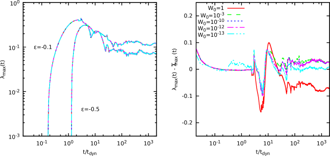
Figure 1: Left panel: Evolution of $\lambda_{\rm max}(t)$ for two orbits with $\mathcal{E}=-0.1$ and $-0.5$ evolved in a frozen Plummer potential generated by $N=10^{5}$ particles for different initial normalizations of the tangent dynamics $\mathbf{W}_{6}$. Right panel: Evolution of the difference $\lambda_{\rm max}(t)-\tilde{\lambda}_{\rm max}(t)$ for the case with $\mathcal{E}=-0.1$ and same choices of the initial normalization.

2.2 Numerical methods and tests

We use an adaptive order symplectic integrator (Kinoshita et al. 1991; Casetti 1995) with fixed time-step $\Delta t$ to solve the equations of motion

$$\ddot{{\mathbf{r}}}_{i}=-Gm\sum_{j=1}^{N}\frac{{\mathbf{r}}_{i}-{\mathbf{r}}_{j}}{||{\mathbf{r}}_{i}-{\mathbf{r}}_{j}||^{3}},$$ (6)

and their associated variational equations for the tangent vectors $\mathbf{w}_{i}$ (Miller 1971; Goodman et al. 1993; Hemsendorf & Merritt 2002; Rein & Tamayo 2016)

$$\ddot{{\mathbf{w}}}_{i}=-Gm\sum_{j=1}^{N}\left[\frac{{\mathbf{w}}_{i}-{\mathbf{w}}_{j}}{||{\mathbf{r}}_{i}-{\mathbf{r}}_{j}||^{3}}-3({\mathbf{r}}_{i}-{\mathbf{r}}_{j})\frac{({\mathbf{w}}_{i}-{\mathbf{w}}_{j})\cdot({\mathbf{r}}_{i}-{\mathbf{r}}_{j})}{||{\mathbf{r}}_{i}-{\mathbf{r}}_{j}||^{5}}\right]$$ (7)

that are needed to compute the Lyapunov exponent (see below). As a rule, we use the 4th order integrator with $\Delta t=10^{-2}t_{\rm dyn}$ for models with $N<3\times 10^{4}$ and the 2nd order integrator with $\Delta t=3.3\times 10^{-3}t_{\rm dyn}$ for larger system sizes. Throughout this work we assume units such that $G=M=r_{c}=1$, so that the dynamical time $t_{\rm dyn}=\sqrt{r_{c}^{3}/GM}$ and the scale velocity $v_{\rm typ}=r_{c}/t_{\rm dyn}$ are also equal to 1. Individual particle masses are then $m=1/N$.
Typically, in direct $N$-body simulations, the divergence of the Newtonian potential for vanishing interparticle separation, leading to the accumulation of round-off errors in the trajectories, is cured by introducing the softening length $\epsilon_{\rm soft}$ so that the potential at distance $r$ from a particle of mass $m$ becomes $\phi(r)=-Gm/\sqrt{r^{2}+\epsilon_{\rm soft}^{2}}$. For our choice of timestep $\Delta t$ we take as optimal value of the softening $\epsilon_{\rm soft}=5\times 10^{-3}r_{c}$ (for a detailed analysis of the relation between the optimal values of $\Delta t$ and $\epsilon_{\rm soft}$, see Dehnen & Read 2011, and references therein). We verified that, at fixed $\epsilon_{\rm soft}$, the results of the numerical simulations are unchanged when further decreasing $\Delta t$. Tracer particle integrations in frozen potentials are extended up to $t=2000\,t_{\rm dyn}$, while self-consistent equilibrium $N$-body simulations to $t=200\,t_{\rm dyn}$, for all the values of $N$. It is worth noting that the softening of the interactions not only cures the numerical problems related to the divergence of the $1/r$ potential when $r\to 0$, but also makes the system “less collisional” than a system with the same $N$ particles but unsoftened interactions, because the strongest collisions where particles become really close to each other have a much smaller impact on the system. However, the two-body relaxation time still grows with $N$ as $t_{2b}\propto N/\ln N$ (see e.g. Gabrielli et al. 2010). Note that, if $\epsilon_{\rm soft}$ is larger than the typical impact parameter of strong encounters (leading to deflections of 90 degrees), then the Coulomb logarithm is no longer proportional to $\ln N$, but becomes the constant $\ln\Lambda=\ln(b_{\rm max}/b_{\rm min})$, where $b_{\rm min}=\epsilon_{\rm soft}$ and $b_{\rm max}$ is typically the scale size of the system, in our case quantified by $r_{c}$. Note also that the introduction of softening does not reduce the collisional relaxation rate much, precisely because softening only affects the Coulomb logarithm, the latter spanning about two decades upon varying $\epsilon_{\rm soft}$ of six decades in units of the typical scale length of the system (see e.g. Hernquist & Barnes 1990 and Dehnen 2001).
As mentioned in the Introduction, a quantitative measure of the degree of chaotic instability of the dynamics is given by the largest Lyapunov exponent, measuring the exponential growth rate of perturbations of a given trajectory in phase space. We compute the numerical estimate of the largest Lyapunov exponent by means of the standard Benettin et al. (1976) method (see also Contopoulos 2002; Ginelli et al. 2007, 2013) as

$$\lambda_{\rm max}(t)=\frac{1}{L\Delta t}\sum_{k=1}^{L}\ln\frac{W(k\Delta t)}{W_{0}}\leavevmode\nobreak\ ,$$ (8)

for a (large) time $t=L\Delta t$, where $W$ is the norm of the $6N$-dimensional vector

$$\mathbf{W}_{6N}=(\mathbf{w}_{i},\dot{\mathbf{w}}_{i},...\mathbf{w}_{N},\dot{\mathbf{w}}_{N}),$$ (9)

for self-consistent simulations, and of the six-dimensional vector

$$\mathbf{W}_{6}=(\mathbf{w},\dot{\mathbf{w}}),$$ (10)

for a tracer in a frozen $N$-body model. In both cases, $W_{0}$ is the value of such norm at $t=0$. The “true” largest Lyapunov exponent would correspond to the limit for $L\to\infty$ in Eq. (8), therefore what we compute is, properly speaking, the finite-time Lyapunov exponent $\lambda_{\rm max}(t)$, that may differ from the true asymptotic value $\lambda_{\rm max}=\lim_{t\to\infty}\lambda_{\rm max}(t)$. However, we checked that $L$ is large enough for the result to appear relaxed to its asymptotic value, so that we may be confident that our long-time results are a good approximation to $\lambda_{\rm max}$. Hereafter, to avoid confusion, we will use $\lambda_{\rm max}$ to denote the largest Lyapunov exponent of a single particle orbit in

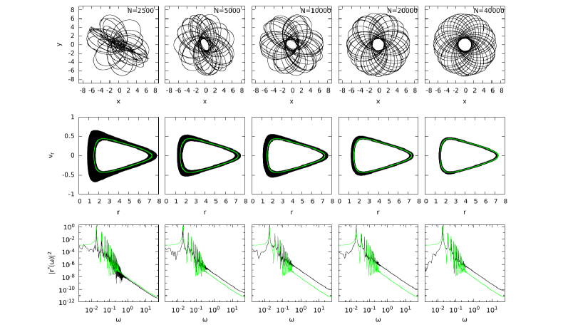
Figure 2: Top row: projections on the $x,y$ plane of five tracer orbits starting with the same initial condition $(\mathbf{r}_{0},\mathbf{v}_{0})$, with energy per unit mass $\mathcal{E}=-0.1$, evolved in a frozen $N$-body potential generated by a discrete Plummer distribution of $N=2.5\times 10^{3}$, $5\times 10^{3}$, $\times 10^{4}$ $2\times 10^{4}$ and $4\times 10^{4}$ particles. Middle row: orbit section in the $r,v_{r}$ plane. Bottom row: squared modulus of the Fourier spectrum of the radial coordinate $r$. In all plots the black lines refer to the discrete models, while the green (gray) ones to the same initial condition propagated in the parent smooth potential.

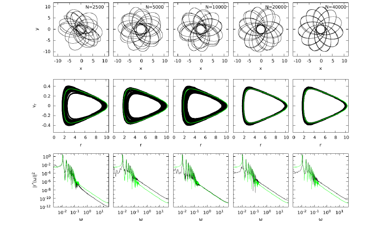
Figure 3: Same as in Fig. 3 but for a Hernquist model.

a frozen or smooth potential, and $\Lambda_{\rm max}$ for the largest Lyapunov exponent of the full $6N$-dimensional self-consistent problem. To improve convergence, following Benettin et al. (1976), the vector $\mathbf{W}_{6N,6}$ is periodically renormalized to $W_{0}$. In all simulations presented here, the renormalization procedure is done every $10\Delta t$. The final value attained by $\lambda_{\rm max}$ (or $\Lambda_{\rm max}$) is independent of the frequency of this operation and the value of $W_{0}$, that we fix to unity in all simulations shown here.
We note that in previous works several authors (see e.g. Sideris 2004; Kandrup et al. 2004; Meschiari 2006) used, in order to evaluate Eq. (8) for a tracer particle, the difference between two realizations of the same orbit starting with initial conditions $(\mathbf{r}_{0},{\mathbf{v}}_{0})$ and $(\mathbf{r}^{\prime}_{0},{\mathbf{v}}^{\prime}_{0})$, i.e. $\tilde{\mathbf{W}}_{6}=(\mathbf{r}-\mathbf{r}^{\prime},{\mathbf{v}}-{\mathbf{v}}^{\prime})$ instead of the tangent vectors. By doing so, the value of the largest Lyapunov exponent $\tilde{\lambda}_{\rm max}$ strongly depends on the choice of $\tilde{W}_{0}$, at variance with its counterpart evaluated using the tangent dynamics that, in general, has a different value and is independent of $W_{0}$ (see e.g.  Mei & Huang 2018). In order to assess the magnitude of such discrepancy, we have performed some test simulations where two realizations of a given trajectory with different initial distance $\tilde{W}_{0}$ in the range $(10^{-13},1)$ were integrated in the frozen potential generated by a distribution of $N$ particles extracted from a Plummer distribution, for various $N$. We computed the largest Lyapunov exponent over $2000\,t_{\rm dyn}$ by means of the standard expression (8) using the tangent vectors, as well as using the difference between the two realizations, having set in all cases $\mathbf{W}_{6}=\tilde{\mathbf{W}}_{6}$ at $t=0$. We observed that, as expected, the values attained by the Lyapunov exponent computed in the “correct” way is independent on the initial value of the norm for all orbit energies and system sizes, as shown in the left panel of Fig. (1) for two particles with initial energies $\mathcal{E}=-0.1$ and $-0.5$ in a frozen Plummer model with $N=10^{5}$. On the contrary, when evaluating $\tilde{\lambda}_{\rm max}$ using the difference between two initially close realizations of the same orbit, its value is significantly different from $\lambda_{\rm max}(t)$ at all times for $\tilde{W_{0}}>10^{-13}$. This is exemplified in the right panel of Fig. (1), where $\lambda_{\rm max}(t)-\tilde{\lambda}_{\rm max}(t)$ is plotted as function of time, and it can be clearly seen to converge to zero only for the smallest choice of $\tilde{W}_{0}$.

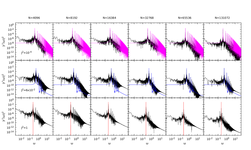
Figure 4: Fourier spectra of radial coordinates of orbits with $\mathcal{E}=-0.8$ propagated in a frozen Plummer model with increasing $N$ and different values of angular momentum $J^{2}=10^{-4}$ (upper panels), $6\times 10^{-2}$ (middle panels), and $1$ (bottom panels). The black curves refer to the orbit in the frozen $N$-body potential, while the coloured (gray) ones to the corresponding orbit propagated in the smooth Plummer potential.

3 Simulations and results

3.1 Orbits in frozen $N$-body potentials

Single particle orbits in frozen $N$-body self-gravitating systems have been extensively used to study the dynamics in triaxial systems for which analytic formulations of the phase-space distribution function are unknown (see e.g. Kandrup et al. 2004; Contopoulos & Harsoula 2013; Manos & Machado 2014; Machado & Manos 2016; Chaves-Velasquez et al. 2017; Patsis & Harsoula 2018, and references therein) and are usually constructed numerically using orbit libraries

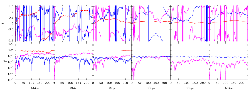
Figure 5: Evolution of the orbital inclination $I$ (top) and squared angular momentum $J^{2}$ (bottom) for the same orbits as in Fig. 4.

(Schwarzschild 1979; Terzić 2002, 2003). It is well known (see e.g. Merritt & Valluri 1996, 1998; Valluri & Merritt 1998) that triaxial potentials are associated to mixed phase-space, admitting regions with both regular and chaotic orbits. When it comes to the study of discrete $N$-body models, it is not always easy to determine on which extent the chaos is due to the discreteness or to the finite deviation from spherical symmetry.
In this paper we study the orbital structure and the scaling of the the largest Lyapunov exponent as a function of the number of particles $N$ in spherical models, starting with their frozen realizations. We have evolved the same initial condition $(\mathbf{r}_{0},\dot{\mathbf{r}}_{0})$ in the frozen $N$-body realizations of Plummer and Hernquist density profiles for $10^{2}\leq N\leq 3\times 10^{7}$. In Figs. 2-3 we show, for Plummer and Hernquist models, respectively, the same initial conditions propagated in the potential of a frozen $N$-body model for $N=2.5\times 10^{3}$, $5\times 10^{3}$, $10^{4}$, $2\times 10^{4}$ and $4\times 10^{4}$. For both models, as $N$ increases the orbit projection in the $x,y$ plane (upper rows) becomes more and more regular and markedly centrophobic (cfr. analogous plots in Kandrup & Sideris 2001; Sideris & Kandrup 2002; Kandrup et al. 2004). Consistently, and as expected, the radial phase-space sections $r,v_{r}$ (middle rows) show that the orbit propagated in the discrete frozen potential (black dots) approaches that in the smooth potential (green/gray dots) for increasing values of $N$. As a general trend, and for both choices of $\rho(r)$ the phase-space sections show a larger diffusion from the “analytic orbit” at low radii and are bound

Figure 6: Ordered plot of the largest Lyapunov exponents for a set of $N_{t}=500$ tracers propagating in frozen $N$-body Plummer potential with $N=10^{2}$, $10^{3}$, $10^{4}$ and $10^{5}$ (main plot). Maximal Lyapunov exponent for an orbit with $\mathcal{E}=-1$ as function of the softening length $\epsilon_{\rm soft}$ for the $N=10^{3}$ and $10^{5}$ casesd (inset).

between two limit curves up to $t=2\times 10^{3}t_{\rm dyn}$ (the time to which the frozen $N$-body integrations are extended). On the other hand, the behaviour of Fourier spectra of the radial coordinate $r$, $|r^{*}(\omega)|^{2}$ (bottom rows) has a less trivial trend with the system size $N$. For both Plummer and Hernquist density profiles, the peak in the spectrum corresponding to the fundamental radial frequency $\omega_{r}$ does not appear to be significantly shifted with respect to that of the orbit in the smooth potential. The low and high frequency tails do not appear to have any significant trend with $N$ for the Plummer model, while appear to reproduce better the spectrum of the orbit integrated in the smooth potential for intermediate $N$ (e.g., $N=10^{4}$ in Fig. 3). For different values of the integration parameters, such as the order of the symplectic integrator, the timestep $\Delta t$ and the softening length $\epsilon_{\rm soft}$, we observe a qualitatively similar behviour, with a net tendency to have a slight shift in the fundamental orbital frequencies for increasing values of $\epsilon_{\rm soft}$.
In general, the mismatch between the Fourier spectra of orbits propagated in analytic smooth potentials and frozen $N$-body space does not decrease for increasing $N$ (at least for the system sizes considered here in the range $10^{2}\div 10^{7}$), but for fixed initial orbit energy (per unit mass) $\mathcal{E}$, orbits starting with higher values of the initial angular momentum $J$ seem to have power spectra more similar to those of the parent analytical orbit. This is represented in Figure 4 where, as an example, we show $|r^{*}(\omega)|^{2}$ for three different initial conditions evolved in a frozen Plummer model. In all cases the orbits have comparable values of energy per unit mass, while the initial angular momentum $\mathbf{J}_{0}$ has significantly different values in the three rows of curves.

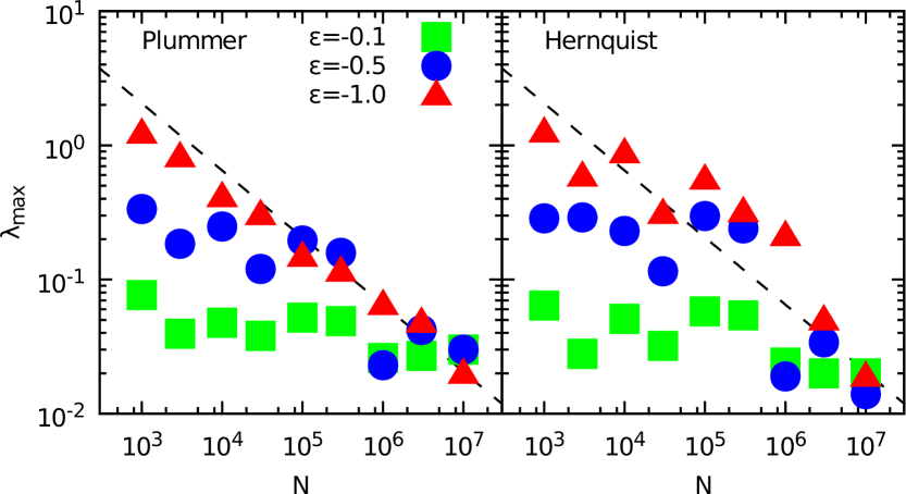
Figure 7: Largest Lyapunov exponent $\lambda_{\rm max}$ for a tracer orbit with ${\mathcal{E}=-0.1,-0.5}$ and $-1$ in a frozen $N$-body model as a function of $N$, for Plummer (left panel) and Hernquist (right panel) profiles. The dashed line is the $N^{-1/2}$ law.

It is evident that for tracer orbits starting with vanishing initial angular momentum (upper row), and the maximum attainable angular momentum (bottom row), increasing the value of $N$ has little effect on improving the matching between the discrete Fourier spectra with that of the orbit in the smooth potential. Only the cases with $N\geq 32768$ and $J_{0}=1$ stand out for not presenting the higher frequency peaks appearing for lower values of $N$. For completeness, in Fig. 5 we present for the same systems of Fig. 4 the evolution of their orbital inclination $I$ (i.e. the angle with respect to the reference plane $z=0$) and squared angular momentum $J^{2}$. It appears clearly that for low angular momentum orbit, the orbital plane undergoes wild oscillations that do not appear to damp out for increasing $N$. The angular momentum modulus itself varies strongly even on time scles as short as $50t_{\rm dyn}$. For orbits starting with large values of $J_{0}$ (closer and closer to the circular orbit with $v_{\rm circ}=\sqrt{rGM(r)}$), the conservation of $J^{2}$ improves for increasing $N$ but the inclination $I$ still presents appreciable changes, reason for which there is still considerable “noise” in the power spectra of $r$ for large values of $N$ in Figs. 2-4. Tuning the force softening $\epsilon_{\rm soft}$ at fixed $N$ and tracer orbit initial parameters reflects on the structure

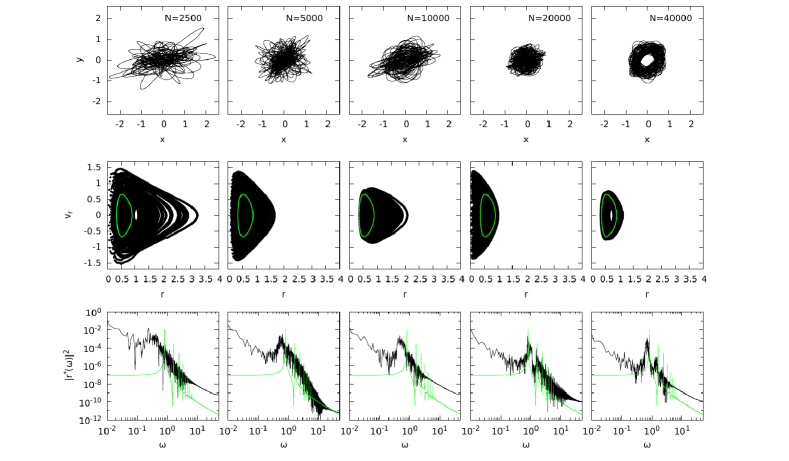
Figure 8: Top row: projections on the $(x,y)$ plane of five tracer orbits starting with the same initial condition $(\mathbf{r}_{0},\mathbf{v}_{0})$, again with initial energy per unit mass $\mathcal{E}=-0.1$ in a self-consistent $N$-body simulation with initial conditions sampled from an isotropic Plummer model with $N=2.5\times 10^{3}$, $5\times 10^{3}$, $\times 10^{4}$ $2\times 10^{4}$ and $4\times 10^{4}$ particles. Middle row: orbit section in the $r,v_{r}$ plane. Bottom row: squared modulus of the Fourier spectrum of the radial coordinate $r$.

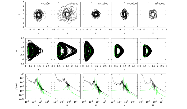
Figure 9: The same as in Fig. 9 for a Hernquist model.

of the power spectra of the radial coordinate $r$ in a shift of the fundamental frequency to slightly lower values of $\omega$ and a narrowing of the associated peak for $\epsilon_{\rm soft}$ increasing towards $0.1r_{c}$ and decreasing towards $10^{-6}r_{c}$ (the limit values of $\epsilon_{\rm soft}$ used in our numerical simulations). For intermediate values (say in the range $3\times 10^{-4}r_{c}<\epsilon_{\rm soft}<3\times 10^{-2}r_{c}$) we do not observe any appreciable variation in the discrepancies with the spectra of the analytical orbit.
For both frozen Plummer and Hernquist models we have evaluated the maximal Lyapunov exponent $\lambda_{\rm max}$ for orbits with different values of the energy per unit mass $\mathcal{E}$ and angular momentum $\mathbf{J}$. As it is evident from Figure 6, where we show the ordered plot of the maximal Lyapunov exponents for $N_{t}=500$ orbits propagated for $10^{3}t_{\rm dyn}$ in frozen Plummer potentials with different values of $N$, where with increasing system size, the distribution of $\lambda_{\rm max}$ of the tracer particles attains systematically lower values. This is particularly evident for the larger values of the Lyapunov exponents, usually associated with smaller values of the orbital energy per unit mass $\mathcal{E}$.
In order to quantify such behaviour as function of $N$ and $\mathcal{E}$, in Figure 7 we show the trend with $N$ of $\lambda_{\rm max}$ for three typical orbital energy values $\mathcal{E}=-0.1,$ $-0.5$, $-1$ obtained averaging over 100 independent realizations. The value of the Lyapunov exponent seems to be almost independent of the number of particles $N$ for weakly bound orbit (i.e., $\mathcal{E}=-0.1$ in this case, see also Fig. 6 for $i/N_{t}\to 0$), while it seems to approach a $\lambda\propto N^{-1/2}$ decay as the tracer orbit is more and more bound, independently of the specific density profile at hand. Moreover, we observe that decreasing the softening length at fixed $N$ is always associated with a systematic increase of the values of $\lambda_{\rm max}$ for the tracer orbit. However, for $\epsilon_{\rm soft}\lesssim l_{\rm int}$ (the mean inter-particle distance within $r_{c}$), the values of the Lyapunov exponents appear to accumulate to a limit value, rather than increasing indefinitely (see inset in Fig. 6).

3.2 Self-consistent equilibrium models

We repeated the analysis described above for active (i.e., their contribution to the force field is accounted) and non-interacting tracer particles with the same initial conditions $(\mathbf{r}_{0},{\mathbf{v}}_{0})$ in self-consistent $N$-body runs with the same values of $N$ (see Figs. 8, 9). We find that, starting from the same initial conditions, an active particle and a tracer particle are virtually indistinguishable for $N>2000$.
From the point of view of the orbital structure, for both Plummer and Hernquist models, the situation in this case is more consistent with what one would expect, with more similar spectra at larger $N$. In particular, as $N$ increases individual particle orbits become more regular (even though less rapidly than in frozen $N$-body models) and explore less and less phase space.
Additionally, we have computed the maximal Lyapunov exponent $\lambda_{\rm max}$ for different tracer particles moving in an active self-consistent model and its frozen $N$-body and smooth orbits counterparts, for both choices of the density profile and different values of energy per unit mass $\mathcal{E}$ and angular momentum $\mathbf{J}$.
The distributions of Lyapunov exponents as a function of the initial particle energy and angular momentum, for fixed profile and system size $N$, are remarkably similar for

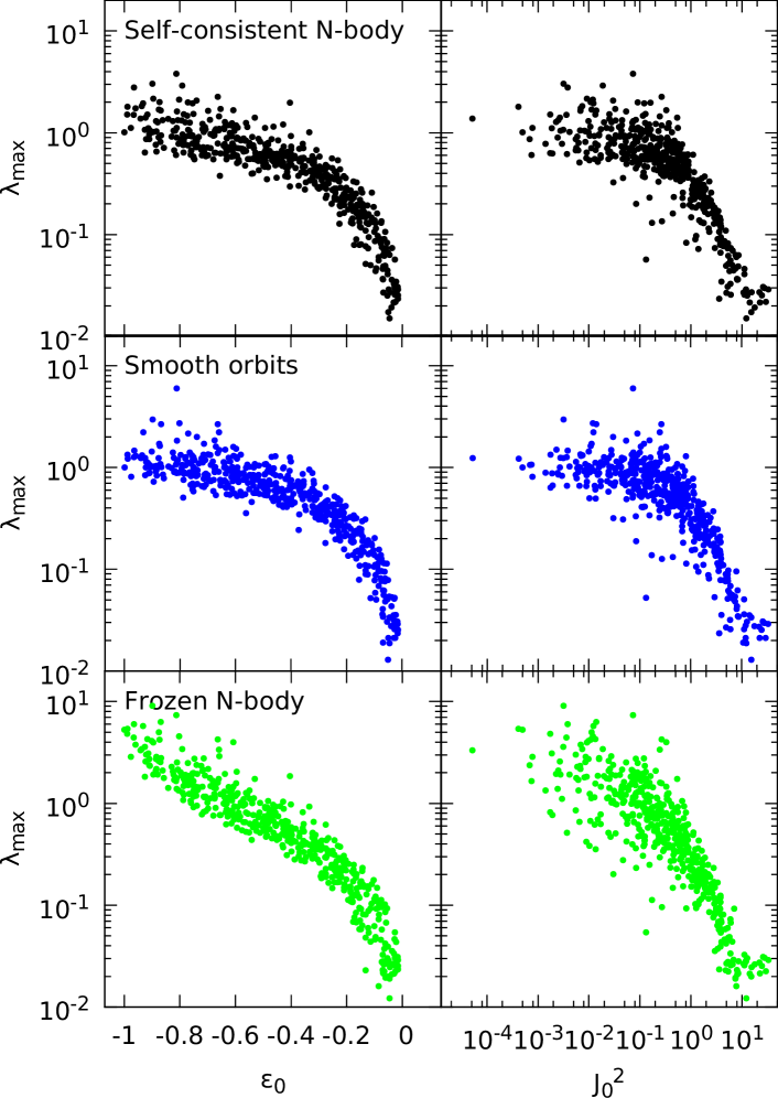
Figure 10: Largest Lyapunov exponent $\lambda_{\rm max}$ for a system of 500 tracer particles moving in a isotropic self-consistent $N$-body model (top panels), in a system of non-interacting particles propagated in a smooth potential (middle panels), and in a frozen $N$-body model (bottom panels), as a function of the initial energy per unit mass $\mathcal{E}_{0}$, (left column) and initial value of the squared angular momentum $J^{2}_{0}$ (right column). In all cases $N=10000$ and Plummer density profile.

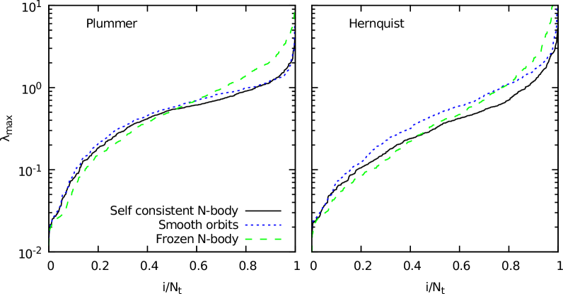
Figure 11: Ordered plot of the largest Lyapunov exponents for a set of $N_{t}=500$ tracers propagating in active $N$-body models (solid lines), non-interacting systems of smooth orbits (dotted lines) and frozen $N$-body potentials (dashed lines), for $N=10000$ and Plummer (left) and Hernquist (right) density profiles.

tracers propagated in self-consistent $N$-body and smooth orbit systems, with the frozen $N$-body case showing instead a different slope in the $\lambda_{\rm max},\mathcal{E}_{0}$ and $\lambda_{\rm max},J^{2}_{0}$ planes, with larger exponents associated with smaller initial energies as shown in Fig. 10 for the $N=10000$ Plummer case. This reflects also in the structure of the ordered plot of $\lambda_{\rm max}$, as presented in Fig. 11 for the Plummer (left) and Hernquist (right) density profiles and $N=10000$ (i.e., the self-consistent

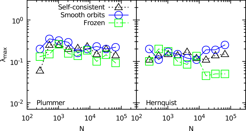
Figure 12: Largest Lyapunov exponent $\lambda_{\rm max}$ for a tracer particle moving in an isotropic self-consistent $N$-body model (triangles), in a system of non-interacting particles propagated in a smooth potential (circles), and in a frozen $N$-body model (squares), as a function of $N$, for Plummer (left panel) and Hernquist (right panel) density profiles.

and smooth orbit cases have the same slopes). In general, we observe again that for weakly bound particles with large angular momentum, the values themselves attained by $\lambda_{\rm max}$ for given $N$ do not present substantial difference from one model to one another, as shown in Fig. 12 for the $\mathcal{E}\simeq-0.3$ and $J^{2}\simeq 2$ case. For $N>10^{4}$ such orbits do not appear to have significant changes in both the magnitude and the orientation of $\mathbf{J}$, as shown in Fig. 13. Vice-versa, the value of $\lambda_{\rm max}$ for tracer particles in self-consistent systems becomes more strongly dependent on the initial energy $\mathcal{E}_{0}$ for more bound particles, the latter having in general more chaotic trajectories.
We interpret all these facts as a hints that the continuum limit shall be questioned at least concerning the concept of $N$-body chaos, in particular, with respect to the usefulness of frozen $N$-body models as surrogates of an equilibrium finite-$N$ body problem. The phase-space transport of initially localized orbit families should be quite different in the two cases since in a frozen model the single particle energy is always conserved independently of $N$, while in active $N$-body models particles could exchange energy, even in the limit $N\to\infty$. This is exemplified in Figs. 14-15 (for Plummer and Hernquist profiles, respectively) where we show at different times ($t=0$, $5$, $10$, 20, 30 and $50\,t_{\rm dyn}$) the positions in the $(x,y)$ and $(x,v_{x})$ planes of an initially localized bunch of $N_{t}=500$ tracers propagated in a $N=20000$ self consistent model (black points), a system of non-interacting particles in a static smooth potential (blue/dark gray points) and a frozen (green/light gray points). Tracer particles in self-consistent simulations rapidly explore a large portion of configuration and phase-space in the Hernquist case (Fig. 15), while they start spreading at later stages, say at around $30t_{\rm dyn}$ in the Plummer case (Fig. 14) for comparable values of initial energies and angular momentum. Tracer particles moving in frozen $N$-body systems or interacting with moving particles in a fixed smooth potential, tend instead to remain clustered for long times in both configuration and phase-spaces,

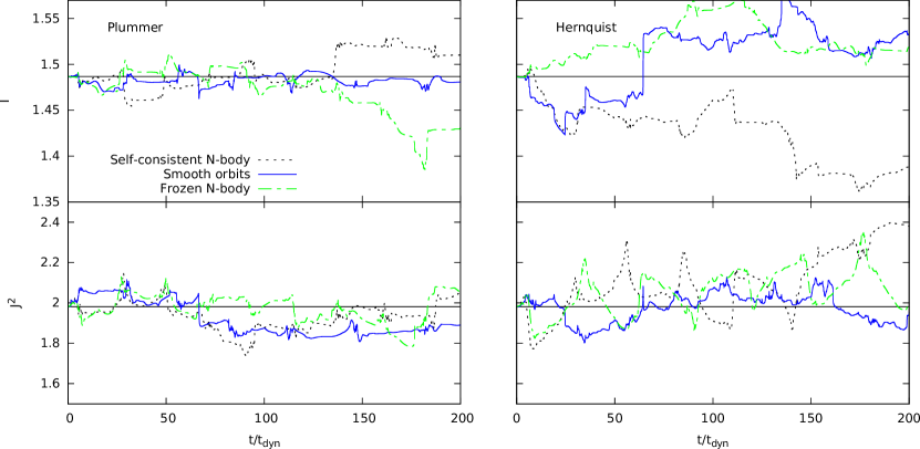
Figure 13: Time evolution of the orbital inclination $I$ (upper panels) and the square of the angular momentum $J^{2}$ (lower panels) for a tracer particle in a frozen $N$-body potential (dotted-dashed lines), a self consistent model (dotted line) and a system of non-interacting orbits moving in a smooth potential (solid lines), for Plummer (left) and Hernquist (right) density profiles. In all cases $N=16348$

with only the case of non-interacting orbits in smooth Hernquist potential showing some considerable spread at $t=50t_{\rm dyn}$. As a matter of fact, this is because self-consistent models do have collective effects, that may also be enhanced by the discreteness-induced noise (Weinberg 1998; El-Zant et al. 2016), while frozen $N$-body models have nothing but intrinsic discreteness noise. The third case, represented by non-interacting orbits moving in a fixed smooth potential, lies in between as its effective field on a tracer particle is time dependent. In order to check whether the spread in phase-space over the integration times is consistent with a diffusive process (associated with two body collisions), we have computed the evolution of the tracers’ mean velocity $\bar{v}$ and root-mean squared velocity $v_{\rm rms}\equiv\sqrt{\sum_{i=1,N_{t}}(v_{i}-\bar{v})^{2}}/N$, as well as their mean energy and angular momentum $\bar{\mathcal{E}}$ and $\bar{J}$. We find that, independently of the density profile, $\bar{v}$ has an oscillatory behaviour while $v_{\rm rms}$ grows logarithmically up to $\sim 20t_{\rm dyn}$, saturating for the frozen $N$-body case and rapidly increasing with a steep power-law trend for the self-consistent and smooth orbit cases. In general, the evolution of the tracer r.m.s. velocity is incompatible with a growth $\propto t^{1/2}$ as expected from a diffusive process à la Chandrasekhar. The evolution of the average CBE invariants, by definition not subjected to phase-mixing at variance with particle velocities, has an oscillatory behaviour in frozen systems independently of $N$, while it is compatible with a power-law for the smooth potential and the self consistent models with $N\lesssim 1000$.
We argue that the discrepancies between analytical orbits in smooth potentials and tracer orbits in frozen and live $N$-body models are essentially an effect of the overall discreteness and chaoticity of the latter potentials, rather than an effective collisional evolution, in direct $N$-body simulations, (see also Habib et al. 1997).
Let us now consider the largest Lyapunov exponent $\Lambda_{\rm max}$ for an active self-consistent model (Fig. 16), and especially its dependence on $N$ and on the nature of the density profile.

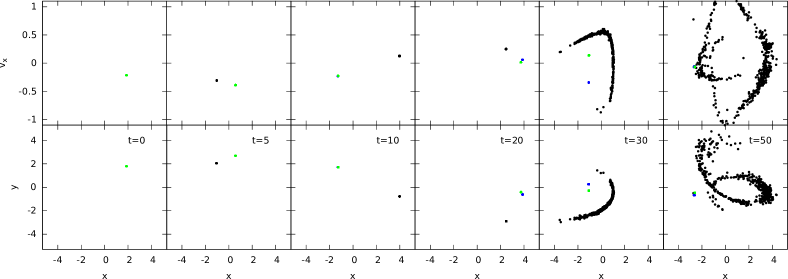
Figure 14: Projections in the $x,v_{x}$ (top row) and $x,y$ planes of a distribution non-interacting tracers propagated in a self-consistent Plummer model (black points), a frozen Plummer model (green/light gray points) and a system of non interacting orbits in a smooth Plummer potential (blue/dark gray points), at (from left to right) $t=0$, 5 10, 20, 30 and 50. In all cases $N=20000$ and $N_{t}=500$.

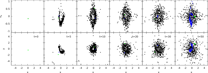
Figure 15: Same as Fig. 14 but for a Hernquist model.

The degree of chaoticity of such a system strongly depends on the nature of the density profile, with cuspy models being in general more chaotic for sufficiently large $N$.
In all cases the largest Lyapunov exponent decreases with $N$ (at least for $N>2\times 10^{3}$) resulting in increasing values of the Lyapunov time (that is, $\Lambda^{-1}_{\rm max}$), that remains within one order of magnitude around the dynamical time. In order to check the whether such behaviour is affected by the short distance regularization of the $1/r^{2}$ force law, we have performed simulations with same initial conditions and different values of the softening length $5\times 10^{-4}\leq\epsilon_{\rm soft}\leq 3\times 10^{-2}$ (and associated optimal timestep, see Dehnen & Read 2011). As expected, larger values of $\epsilon_{\rm soft}$ results in lower values of $\Lambda_{\rm max}$ for fixed density profile and particle number $N$. Curiously, for the Plummer model (left pannel in Fig. 16) we observe a slight increase of $\Lambda_{\rm max}$ with $N$ for the smaller value of $\epsilon_{\rm soft}\approx 10^{-3}$ for $N<2\times 10^{3}$. We verified that such increase holds for even smaller values of the softening length (yielding remarkably similar values of $\Lambda_{\rm max}$, not pictured here), however what happens in this case for larger values of $N$ is left undetermined, due to the prohibitively small values of the associated optimal timestep $\Delta t$ to be used for the simulations. We conjecture that this latter issue might have led to speculate that $\Lambda_{\rm max}$, and more in general the Lyapunov exponent associated to single particle trajectories are indeed constant or slightly increasing functions of $N$. Remarkably, for sufficiently small values of the softening length we find evidence of a crossover between a Lyapunov exponent nearly constant with $N$ at small $N$’s and a decreasing one at larger $N$’s, as suggested by Goodman et al. (1993) and El-Zant et al. (2019). Such a behaviour is apparent for the Plummer case and less evident in the Hernquist case. However, even considering smaller softening lengths than those of the data shown in Fig. 16, we do not find clear evidences of a threshold $\epsilon_{c}$ between constant and decreasing $\Lambda(N)$ depending on $N$ as $\epsilon_{c}\sim r_{c}/\sqrt{N}$.
As a general trend, in the Plummer case the $N$-dependence of $\Lambda_{\rm max}$ at large $N$ is well described by a $N^{-1/2}$ law (solid lines in Fig.  16), while in the Hernquist case the $N$-dependence is weaker and, although the values are consistently decreasing up to $N\approx 10^{5}$, a saturation for large values of $N$ or a matching with a $N^{-1/3}$ law (dashed lines in Fig.  16) can not be totally ruled out by our results. We recall that a $\Lambda_{\rm max}\propto N^{-1/3}$ behaviour for softening lengths larger than the threshold $\epsilon_{c}$ was estimated by Goodman et al. (1993) and also by Gurzadyan & Savvidy (1986), in the latter case using a differential geometry approach to the gravitational $N-$body problem.
We note that our results for $\Lambda_{\rm max}$ are given in units of $t^{-1}_{\rm dyn}$, that, as mentioned above, is always equal to unity. Cipriani & Pettini (2003) introduced a dimensionless maximal Lyapunov exponent or “dimensionless chaoticity indicator” as $\gamma_{1}\equiv\Lambda_{\rm max}t_{\rm dyn}$. Such quantity, at variance with $\Lambda_{\rm max}$ computed here, was found to be independent of $N$ and on the average particle energy. Note that, however, the value of $t_{\rm dyn}=\sqrt{G\rho}$ used by Cipriani & Pettini (2003) depends on the mass density $\rho$ that we keep fixed, while in their case varies as a function of $N$, thus restoring a dependence on the number of particles of the dynamical time.

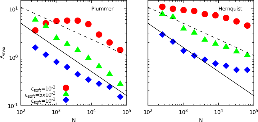
Figure 16: Largest Lyapunov exponent $\Lambda_{\rm max}$ for an isotropic self-consistent $N$-body model as function of $N$ and different values of the force softening $\epsilon_{\rm soft}$, for Plummer (left panel) and Hernquist (right) density profiles. The solid and dashed lines mark the theoretical $N^{-1/2}$ and $N^{-1/3}$ laws, respectively.

4 Summary and conclusions

We have investigated the chaotic properties of the dynamics of $N$-body self-gravitating systems, studying single-particle orbits in frozen and active potentials as well as the dynamics in the full $6N$-dimensional phase space. Initial conditions were always drawn from spherically symmetric stationary models, namely, the flat-cored Plummer model and the centrally cuspy Hernquist model. The main results of this study can be summarized as follows.
As to the properties of single-particle orbits, the orbital structure of particles in frozen $N$-body models approaches that of continuum potentials, however the dependence on $N$ of this trend is not trivial. Moreover, orbits in frozen models and active self-consistent models have (obviously) different mixing properties and have, typically, different largest Lyapunov exponents; the dependence of the largest Lyapunov exponent on $N$ is more pronounced in frozen systems than in active ones.
In general, the differences between an orbit propagated in a frozen model or in a live $N$-body model and their smooth potential counterpart become evident already after a few dynamical times, therefore on a scale much smaller than the collisional relaxation time $t_{2b}$. For example, for the model with $N=40000$, the integration time of 200$t_{\rm dyn}$ is roughly equal to $0.1t_{2b}$, ruling out the dynamical collisions (in the sense of Chandrasekhar theory) as the origin of the differences with the analytical orbits in the smooth potential. We therefore conjecture that the nature of the fluctuations in the full N-body potential, and possibly their scales and space time correlations, induces an effect on the orbital evolution of particles that challenges the picture of independent, additive, local impulse perturbations assumed in the diffusion process underlying the Chandrasekhar description. Remarkably, at fixed $N$ the differences between orbits in frozen and live $N$-body potentials depend on the specific orbital parameters at hand. In general, orbits with lower initial angular momentum evolve more in the live case, where an excursion in both $J$ and $\mathcal{E}$ is possible.
Given that orbits in potentials that are integrable in the continuum limit behave differently in frozen and self-consistent simulations, we argue that nothing can be safely deduced from studies with tracer particles in frozen $N$-body models reproducing non-integrable models, such as, for example, triaxial systems.
As far as the chaotic properties of the dynamics in the full $6N$-dimensional phase space is concerned, our results confirm the expectation (and previous results, at least qualitatively; see e.g. El-Zant 2002) that systems with larger $N$ are less chaotic. However, the actual value of the largest Lyapunov exponent as well as its dependence on $N$ depend on the chosen equilibrium model: the flat-cored Plummer model has smaller Lyapunov exponents that are proportional to $N^{-1/2}$, while the Lyapunov exponents of the cuspy Hernquist model are systematically larger than the Plummer ones and their dependence on $N$ is considerably weaker. The values of the largest Lyapunov exponent obviously depend on the softening length, given that systems with different softenings are different dynamical systems; as expected, smaller softening lengths yield larger Lyapunov exponents, i.e., more chaotic systems. This notwithstanding, the Lyapunov exponent does decrease with increasing $N$, at least for sufficiently large $N$’s. The dynamical behaviour is thus consistent with a regular (non-chaotic) behaviour in the continuum ($N\to\infty$) limit, although no numerical experiment can obviously prove that unambiguously.
It is important to stress that we considered only systems with a finite softening length, being interested in investigating the relation with the collisionless limit, that requires a finite softening length. Our results cannot be extrapolated to the unsoftened case, hence are not in contradiction with previous results on the degree of chaoticity by Goodman et al. (1993), Hemsendorf & Merritt (2002) and El-Zant et al. (2019), that seem to suggest a $\Lambda_{\rm max}$ independent of $N$ for the unsoftened gravitational $N-$body problem. We note that the rôle played by softening in affecting chaos in self-gravitating systems had been also studied by Komatsu et al. (2009), that found a linear decrease of $\Lambda_{\rm max}$ with increasing $\epsilon_{\rm soft}$ at fixed $N$.
This established, it remains to clarify whether the present results could be extended to axisymmetric and triaxial models (admitting in the continuum limit the coexistence of regions of regular and chaotic dynamics), or spherical models with velocity anisotropy. The interplay between $N$-body chaos and external noise in models characterized by Osipkov-Merritt radial anisotropy will be explored in a forthcoming publication.

References

- Antoni & Ruffo (1995) Antoni M., Ruffo S., 1995, Phys. Rev. E, 52, 2361
- Benettin et al. (1976) Benettin G., Galgani L., Strelcyn J.-M., 1976, Phys. Rev. A, 14, 2338
- Benhaiem et al. (2018) Benhaiem D., Joyce M., Sylos Labini F., Worrakitpoonpon T., 2018, MNRAS, 473, 2348
- Binney & Tremaine (2008) Binney J., Tremaine S., 2008, Galactic Dynamics: Second Edition. Princeton University Press
- Campa et al. (2009) Campa A., Dauxois T., Ruffo S., 2009, Physics Reports, 480, 57
- Campa et al. (2014) Campa A., Dauxois T., Fanelli D., Ruffo S., 2014, Physics of Long-Range Interacting Systems. Oxford University Press, Oxford
- Casetti (1995) Casetti L., 1995, Phys. Scr., 51, 29
- Casetti et al. (1996) Casetti L., Clementi C., Pettini M., 1996, Phys. Rev. E, 54, 5969
- Casetti et al. (2000) Casetti L., Pettini M., Cohen E. G. D., 2000, Physics Reports, 337, 237
- Cerruti-Sola & Pettini (1995) Cerruti-Sola M., Pettini M., 1995, Phys. Rev. E, 51, 53
- Chandrasekhar (1941) Chandrasekhar I. S., 1941, ApJ, 93, 285
- Chaves-Velasquez et al. (2017) Chaves-Velasquez L., Patsis P. A., Puerari I., Skokos C., Manos T., 2017, ApJ, 850, 145
- Cipriani & Pettini (2003) Cipriani P., Pettini M., 2003, Ap&SS, 283, 347
- Contopoulos (2002) Contopoulos G., 2002, Order and chaos in dynamical astronomy
- Contopoulos & Harsoula (2013) Contopoulos G., Harsoula M., 2013, MNRAS, 436, 1201
- Dehnen (2001) Dehnen W., 2001, MNRAS, 324, 273
- Dehnen & Read (2011) Dehnen W., Read J. I., 2011, European Physical Journal Plus, 126, 55
- Di Cintio (2014) Di Cintio P., 2014, PhD thesis, Technische Universität Dresden (arXiv:1408.3857)
- Eddington (1916) Eddington A. S., 1916, MNRAS, 76, 572
- El-Zant (2002) El-Zant A. A., 2002, MNRAS, 331, 23
- El-Zant et al. (2016) El-Zant A. A., Freundlich J., Combes F., 2016, MNRAS, 461, 1745
- El-Zant et al. (2019) El-Zant A. A., Everitt M. J., Kassem S. M., 2019, MNRAS, 484, 1456
- Elskens et al. (2014) Elskens Y., Escande D. F., Doveil F., 2014, European Physical Journal D, 68, 218
- Escande et al. (2018) Escande D. F., Bénisti D., Elskens Y., Zarzoso D., Doveil F., 2018, Reviews of Modern Plasma Physics, 2, 9
- Filho et al. (2018) Filho L. H. M., Amato M. A., Rocha Filho T. M., 2018, Journal of Statistical Mechanics: Theory and Experiment, 3, 033204
- Gabrielli et al. (2010) Gabrielli A., Joyce M., Marcos B., 2010, Physical Review Letters, 105, 210602
- Genel et al. (2019) Genel S., et al., 2019, ApJ, 871, 21
- Ginelli et al. (2007) Ginelli F., Poggi P., Turchi A., Chaté H., Livi R., Politi A., 2007, Physical Review Letters, 99, 130601
- Ginelli et al. (2011) Ginelli F., Takeuchi K. A., Chaté H., Politi A., Torcini A., 2011, Phys. Rev. E, 84, 066211
- Ginelli et al. (2013) Ginelli F., Chaté H., Livi R., Politi A., 2013, Journal of Physics A Mathematical General, 46, 254005
- Goodman et al. (1993) Goodman J., Heggie D. C., Hut P., 1993, ApJ, 415, 715
- Grech et al. (2011) Grech M., et al., 2011, Phys. Rev. E, 84, 056404
- Gurzadyan & Kocharyan (2009) Gurzadyan V. G., Kocharyan A. A., 2009, A&A, 505, 625
- Gurzadyan & Savvidy (1986) Gurzadyan V. G., Savvidy G. K., 1986, A&A, 160, 203
- Habib et al. (1997) Habib S., Kandrup H. E., Elaine Mahon M., 1997, ApJ, 480, 155
- Helmi & Gomez (2007) Helmi A., Gomez F., 2007, preprint, (arXiv:0710.0514)
- Hemsendorf & Merritt (2002) Hemsendorf M., Merritt D., 2002, ApJ, 580, 606
- Hernquist (1990) Hernquist L., 1990, ApJ, 356, 359
- Hernquist & Barnes (1990) Hernquist L., Barnes J. E., 1990, ApJ, 349, 562
- Joyce & Marcos (2007a) Joyce M., Marcos B., 2007a, Phys. Rev. D, 75, 063516
- Joyce & Marcos (2007b) Joyce M., Marcos B., 2007b, Phys. Rev. D, 76, 103505
- Kandrup (1995) Kandrup H. E., 1995, Astronomical and Astrophysical Transactions, 7, 225
- Kandrup (1998a) Kandrup H. E., 1998a, ApJ, 500, 120
- Kandrup (1998b) Kandrup H. E., 1998b, Annals of the New York Academy of Sciences, 848, 28
- Kandrup (2001) Kandrup H. E., 2001, MNRAS, 323, 681
- Kandrup & Mahon (1993) Kandrup H. E., Mahon M. E., 1993, in Buchler J. R., Kandrup H. E., eds, Annals of the New York Academy of Sciences Vol. 706, Stochastic Processes in Astrophysics. p. 81, doi:10.1111/j.1749-6632.1993.tb24683.x
- Kandrup & Novotny (2004) Kandrup H. E., Novotny S. J., 2004, Celestial Mechanics and Dynamical Astronomy, 88, 1
- Kandrup & Sideris (2001) Kandrup H. E., Sideris I. V., 2001, Phys. Rev. E, 64, 056209
- Kandrup & Sideris (2003) Kandrup H. E., Sideris I. V., 2003, ApJ, 585, 244
- Kandrup & Siopis (2003) Kandrup H. E., Siopis C., 2003, MNRAS, 345, 727
- Kandrup et al. (2003) Kandrup H. E., Vass I. M., Sideris I. V., 2003, MNRAS, 341, 927
- Kandrup et al. (2004) Kandrup H. E., Sideris I. V., Bohn C. L., 2004, Physical Review Special Topics Accelerators and Beams, 7, 014202
- Kinoshita et al. (1991) Kinoshita H., Yoshida H., Nakai H., 1991, Celestial Mechanics and Dynamical Astronomy, 50, 59
- Komatsu et al. (2009) Komatsu N., Kiwata T., Kimura S., 2009, Physica A Statistical Mechanics and its Applications, 388, 639
- Lichtenberg & Lieberman (1992) Lichtenberg A., Lieberman M., 1992, Regular and Chaotic Dynamics
- Machado & Manos (2016) Machado R. E. G., Manos T., 2016, MNRAS, 458, 3578
- Manos & Machado (2014) Manos T., Machado R. E. G., 2014, MNRAS, 438, 2201
- Manos & Ruffo (2011) Manos T., Ruffo S., 2011, Transport Theory and Statistical Physics, 40, 360
- Mei & Huang (2018) Mei L., Huang L., 2018, Computer Physics Communications, 224, 108
- Merritt & Valluri (1996) Merritt D., Valluri M., 1996, ApJ, 471, 82
- Merritt & Valluri (1998) Merritt D., Valluri M., 1998, Annals of the New York Academy of Sciences, 858, 48
- Meschiari (2006) Meschiari S., 2006, Master’s thesis, Bologna University
- Miller (1964) Miller R. H., 1964, ApJ, 140, 250
- Miller (1971) Miller R. H., 1971, Journal of Computational Physics, 8, 449
- Monechi & Casetti (2012) Monechi B., Casetti L., 2012, Phys. Rev. E, 86, 041136
- Patsis & Harsoula (2018) Patsis P. A., Harsoula M., 2018, A&A, 612, A114
- Plummer (1911) Plummer H. C., 1911, MNRAS, 71, 460
- Rein & Tamayo (2016) Rein H., Tamayo D., 2016, MNRAS, 459, 2275
- Roy & Perez (2004) Roy F., Perez J., 2004, MNRAS, 348, 62
- Saalmann et al. (2013) Saalmann U., Mikaberidze A., Rost J. M., 2013, Physical Review Letters, 110, 133401
- Schwarzschild (1979) Schwarzschild M., 1979, ApJ, 232, 236
- Sellwood & Debattista (2009) Sellwood J. A., Debattista V. P., 2009, MNRAS, 398, 1279
- Sideris (2002) Sideris I. V., 2002, PhD thesis, UNIVERSITY OF FLORIDA
- Sideris (2004) Sideris I. V., 2004, Celestial Mechanics and Dynamical Astronomy, 90, 147
- Sideris & Kandrup (2002) Sideris I. V., Kandrup H. E., 2002, Phys. Rev. E, 65, 066203
- Sideris & Kandrup (2004) Sideris I. V., Kandrup H. E., 2004, ApJ, 602, 678
- Sylos Labini et al. (2015) Sylos Labini F., Benhaiem D., Joyce M., 2015, MNRAS, 449, 4458
- Terzić (2002) Terzić B., 2002, PhD thesis, THE FLORIDA STATE UNIVERSITY
- Terzić (2003) Terzić B., 2003, preprint, (arXiv:0305.005)
- Terzić & Kandrup (2003) Terzić B., Kandrup H. E., 2003, preprint, (arXiv:0312.434)
- Tsuchiya & Gouda (2000a) Tsuchiya T., Gouda N., 2000a, in Gurzadyan V. G., Ruffini R., eds, The Chaotic Universe. pp 259–267, doi:10.1142/9789812793621˙0016
- Tsuchiya & Gouda (2000b) Tsuchiya T., Gouda N., 2000b, Phys. Rev. E, 61, 948
- Valluri & Merritt (1998) Valluri M., Merritt D., 1998, ApJ, 506, 686
- Weinberg (1998) Weinberg M. D., 1998, MNRAS, 297, 101
- Zerbe et al. (2018) Zerbe B. S., Xiang X., Ruan C.-Y., Lund S. M., Duxbury P. M., 2018, Physical Review Accelerators and Beams, 21, 064201