Accepted for publication in JATIS arXiv preprint typeset using template Stylish-Article⁺ Gamma-ray burst localisation strategies for the SPHiNX hard X-ray polarimeter L. Heckmann¹, N. K. Iyer^2,3*, M. Kiss^2,3, M. Pearce^2,3, F. Xie^2,3† polarimeters — x-rays — gamma ray bursts — Monte-Carlo simulations — analysis techniques SPHiNX is a proposed gamma-ray burst (GRB) polarimeter mission operating in the energy range 50-600 keV with the aim of studying the prompt emission phase. The polarisation sensitivity of SPHiNX reduces as the uncertainty on the GRB sky position increases. The stand-alone ability of the SPHiNX design to localise GRB positions is explored via Geant4 simulations. Localisation at the level of a few degrees is possible using three different routines. This results in a large fraction ($>$ 80%) of observed GRBs having a negligible ($<5\%$) reduction in polarisation sensitivity due to the uncertainty in localisation.

1 Introduction

Gamma-ray bursts (GRB) were serendipitously discovered over 50 years ago by Vela satellites deployed to monitor the ban on nuclear tests in space (Klebesadel et al., 1973). They are now known to be the brightest events in the electromagnetic universe, occurring approximately once per day at random locations on the sky (Paciesas et al., 1999; Bhat et al., 2016). GRBs are thought to be formed during the collapse of a massive object into a black hole (Mészáros, 2006). Two highly relativistic back-to-back plasma jets are produced aligned with the rotational axis of the black hole. The electromagnetic signature of a jet oriented in the earth-direction is detected by instruments as a GRB. Such observations reveal that the emission exhibits a high-energy (keV–MeV) prompt phase (seconds to minutes duration) caused by energy dissipation within the jet; and, a lower energy afterglow (days duration) created by interactions between the burst ejecta and interstellar gas. Both phases have been extensively studied. A relatively coherent description of the afterglow has emerged, but there are still fundamental open questions concerning the underlying physical processes behind the prompt emission (Kumar & Zhang, 2015).

Measurements of the linear polarisation of prompt emission can discriminate between these emission models without the degeneracies associated with modeling of spectral and temporal observations (Toma et al., 2009). Linear polarisation is described by: $(i)$ the polarisation fraction (PF, %) describing the magnitude of beam polarisation; and, $(ii)$ the polarisation angle (PA, degrees) defining the orientation of the electric field vector. Reliable measurements require purpose-built and well-calibrated instruments, and only rudimentary polarimetric observations have been performed to date (McConnell, 2017). A particular challenge is that the polarimetric response of the instrument depends on the relative location of the GRB (Muleri, 2014). Thus localisation strategies become important for instruments studying GRB polarisation. Localisation is also important for multi-wavelength/messenger studies of GRBs. This is exemplified by the recent multi-messenger observation campaign for GRB170817A (Abbott et al., 2017a). Localising this burst with an accuracy of a few degrees using Fermi GBM (Meegan et al., 2009) played an important role in enabling searches with other telescopes (Abbott et al., 2017b).

SPHiNX is a hard X-ray polarimeter (50–600 keV) proposed for the Swedish InnoSat small satellite platform (Pearce et al., 2019). The main objective of the SPHiNX mission is to obtain statistically significant polarisation measurements for a large number of GRBs ($\sim$50) to enable discrimination between GRB prompt emission models. This is achieved through a large field of view (120^∘ cone angle), high polarisation sensitivity and two years of operation in orbit.

The GRB localisation performance of SPHiNX is studied in this paper. The SPHiNX mission and methodology for high-energy polarimetry is described in Section 2. In Section 3, the principle used to localise GRBs is outlined. Details of the methods used for localisation and obtained results are given in Section 4. The paper concludes with a discussion and conclusions in Sections 5 and 6, respectively.

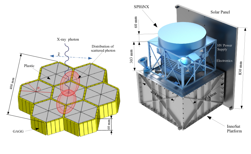
(a)                                                                        (b)

Figure 1: SPHiNX mission : (a) Azimuthal distribution of the scattered photon projected on the SPHiNX scintillator assembly. Detector angle $\phi_{d}$ (see Section 4.2) is also shown. (b) Depiction of the SPHiNX payload as assembled on the InnoSat platform.

2 The SPHiNX mission proposal

SPHiNX utilises Compton scattering of incident photons within a scintillator assembly to estimate the polarisation properties. The interaction cross-section for Compton scattering is described by the Klein-Nishina relationship,

$$\frac{d\sigma}{d\Omega}=\frac{1}{2}r_{e}^{2}\frac{k^{2}}{k_{0}^{2}}\left(\frac{k}{k_{0}}+\frac{k_{0}}{k}-2\sin^{2}\theta\,\cos^{2}\phi\right),$$ (1)

where $r_{e}$ is the classical electron radius, $k_{0}$ and $k$ are the momenta of the incoming and scattered photon, and $\theta$ and $\phi$ are polar and azimuthal scattering angles defined relative to the co-ordinate axes made with the direction and plane of polarisation of the incident photon. X-rays will preferentially scatter in a direction perpendicular to the polarisation vector, as depicted in Fig. 1(a). The polarisation of hard X-rays can therefore be determined in a segmented detector by determining the angle through which the Compton scattering occurs.

The SPHiNX polarimeter comprises 162 detector units (42 plastic and 120 GAGG scintillator units), arranged as shown in Fig. 1(a). The periphery of the scintillators is covered by a contour hugging multi-layered metal shield (of 60 mm height) to reduce the background counting rate. The polarimeter design is optimised to have high polarisation sensitivity whilst satisfying the InnoSat mission constraints, resulting in a flat pixelated geometry (Fig. 1).

The polarisation parameters of incident photons are determined by identifying coincident Compton scattering (preferentially occurring in the low atomic number plastic) and photoelectric absorption interactions (preferentially occurring in the GAGG). Such a combination of scintillator interactions results in double-hit events and defines the azimuthal scattering angle $\phi$. The distribution of $\phi$ is a harmonic function referred to as a modulation curve, where the phase defines PA. PF is defined as $M$/$M_{100}$, where $M$ is the measured modulation amplitude and $M_{100}$ is the modulation amplitude for a 100% polarised beam.

It has become standard to express the polarimetric sensitivity at a 99% ($\sim$3$\sigma$) confidence level in terms of the Minimum Detectable Polarisation (MDP) (Weisskopf et al., 2010),

$$\mathrm{MDP}=\frac{4.29}{M_{100}\,R_{s}}\sqrt{\frac{R_{s}+R_{b}}{T}},$$ (2)

where $R_{s}$ ($R_{b}$) is the signal (background) rate (Hz) and $T$ is the duration of the burst observation (s). There is a 1% probability for an unpolarised GRB to yield PF $>$ MDP through statistical fluctuations. For a given GRB, the value of $M_{100}$ will depend on the location of the GRB with respect to the polarimeter since the modulation pattern depends on the direction from which the detector array is illuminated. An on-axis GRB will produce a sinusoidal modulation curve, whereas distortions will be introduced and the modulation amplitude will decrease as the GRB moves off-axis. This effect is illustrated in Fig. 2 for SPHiNX.

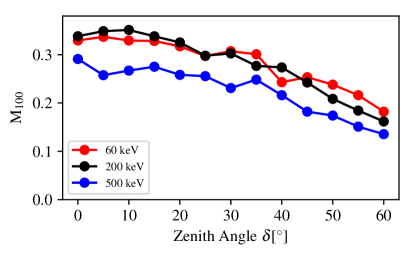
Figure 2: Variation in $M_{100}$ for the SPHiNX detector with incoming photon zenith angle. Values are obtained from simulations described in Pearce et al. (2019).

Once the GRB location is known relative to SPHiNX, the value of $M_{100}$ is determined from computer simulations validated at discrete energies by laboratory measurements (Chauvin et al., 2017). Any uncertainty in the GRB localisation will propagate to an uncertainty in PF,PA and increase the MDP (reduce sensitivity). This is the key difference between GRB polarimeters and on-axis pointed polarimeters for which the source direction is known and fixed for all measurements. Uncertainty in localising these GRBs will also lower the number of GRBs for which significant polarisation measurements can be obtained (due to an increase in MDP). This can diminish the scientific potential for SPHiNX as is seen from Fig. 3.

Figure 3: Effect of uncertainty in source position (zenith angle) on the MDP. Results are obtained by Monte-Carlo sampling of GRBs uniformly distributed in SPHiNX field of view.

Some of the GRBs observed by SPHiNX will be simultaneously observed by other missions. In this case, the GRB sky position can be determined through the Gamma-ray Coordination Network (GCN) and Interplanetary Network (IPN). In this paper, we explore the stand-alone accuracy with which SPHiNX can localise GRBs. The InnoSat mission parameters (e.g. downlink cadence, on-board data processing and storage limits) mean that the localisation would be performed on-ground when data is downloaded once per day. The localisation methods discussed in this paper are, however, sufficiently generic and may be implemented on-board in real-time for missions without such constraints.

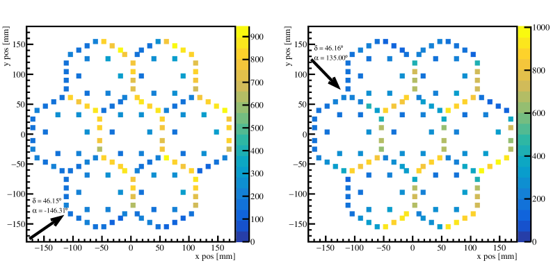
(a) ${\delta}=46.1^{\circ},\,{\alpha}=-146.3^{\circ}$                                         (b) ${\delta}=46.1^{\circ},\,{\alpha}=135^{\circ}$

Figure 4: Variation in counts in different detector units with different source positions. Each detector unit is represented by a single point placed at the center of the unit position.

3 Localisation principle

Hard X-rays interacting in segmented detectors generate an interaction pattern dependent on the incidence direction of photons. This can be used to obtain the photon source direction. Previous GRB missions have either used coded masks (Barthelmy et al., 2005; Bhalerao et al., 2017) or physically separated detector units oriented in different directions (Meegan et al., 2009; Fishman et al., 1982) to obtain distinct interaction patterns.

SPHiNX records direct interactions (single-hit events) as well as scattered interactions (multi-hit events) from incoming photons. Using scattered photons to localise the GRB is difficult as the initial photon direction information is smeared when the photon scatters. Single-hit events preserve the photon direction information and can be used to determine the source location. A GRB observed by SPHiNX will result in a distribution of single-hit counts in the detector units dependent on the relative location of the GRB. Such a detected count map is illustrated in Fig. 4. The GRB location on sky can then be determined by inverting this count map. SPHiNX is sensitive to the photon direction as each detector unit is shielded to different extents (by the metallic shield and by other detector units). The use of a flat geometry reduces sensitivity to the zenith angle of incident photons (especially for a source at a large off-axis position).

This paper focuses on exploring three different inversion routines to obtain the GRB position from the count map. To simplify the problem, all inversion routines assume that a majority of the detected counts come from a single point source in the sky, with counts from other sources forming a part of the diffuse sky background. This is a reasonable assumption since the GRB is momentarily the brightest source in the sky.

The source position is defined using the azimuth ($\alpha$) and zenith ($\delta$) angles of the source with respect to SPHiNX. Uncertainties in the obtained source position are a result of assumptions in the inversion routines and Poisson fluctuations in the detected counts. Each routine gives a set of estimated position angles ($\hat{\alpha}$ and $\hat{\delta}$), uncertainties ($\sigma_{\alpha}$ and $\sigma_{\delta}$) and offsets ($\partial_{\alpha}=|\alpha-\hat{\alpha}|$ and $\partial_{\delta}=|\delta-\hat{\delta}|$) from the actual position. The offsets and uncertainties are used later to compare different routines. The polarisation sensitivity is dependent mainly on $\sigma_{\delta}$, with ${\sigma_{\delta}}\lesssim$ 5^∘ required to minimise the effects of increased MDP in SPHiNX (see Fig. 3). The hexagonal design results in a high degree of azimuthal symmetry and reduces dependence of $M_{100}$ on the azimuthal angle. Thus, polarisation sensitivity is mostly independent of $\sigma_{\alpha}$ and any errors caused by this weak dependence can be added as systematic errors on polarisation values as proposed in Yonetoku et al. (2011).

4 Routine implementation and results

The routines perform an inversion by first obtaining a mapping function between detected counts and sky position. This function is approximated by an empirical relation in one routine and by a pre-computed lookup table in the other two routines.

In order to evaluate the routines (and compute the lookup table), a Monte-Carlo simulation of the SPHiNX polarimeter based on Geant4 (version 10.02.p02) (Allison et al., 2016) is used. Details of the simulation set-up (physics lists, mass model and event selection logic) are given in Refs 27; 20. The Geant4 model used for this simulation is shown in Fig. 5. Simulated photons are emitted from a disk of radius 20 cm located at different positions in the SPHiNX field of view. ROOT (Antcheva et al., 2009) is used both for handling the output data from Geant4 and for implementing the routines to perform the inversion. The data stored from each simulation run consists of hit information of each event such as deposit energy, incident photon direction, detector unit in which the hit occurred and incident energy stored in ROOT Trees.

Figure 5: View of the model used for Geant4 simulations. All components such as the satellite platform, shielding materials, scintillators, electronic read-out boards and solar panel have been included in the model.

The inversion routines are evaluated by simulating a GRB in the SPHiNX field of view. GRB-120107A (with Band parameter $\alpha=-0.94$, $\beta=-2.39$ and $\mathrm{E_{p}}=201.22$ keV) is chosen as a representative GRB for testing the inversion routines. The choice of this representative GRB is not critical as effects of differing GRB spectra are corrected for (see Section 4.3). Effects of changing fluence and position (in sky) are evaluated by simulating the representative GRB with the parameters shown in Table 1.

Table 1: Fluence and position ($\alpha,\delta$) values for evaluating routines

Fluence	$\alpha$	$\delta$	Remarks
2 ph/cm2 to 200 ph/cm2	-54∘	32.8∘	Evaluates the effect of GRB fluence (in 50-300 keV) for weak (2 ph/cm2), median (20 ph/cm2) and very strong GRBs (200 ph/cm2).
14.5 ph/cm2	-180∘ to 180∘.	$43.7^{\circ}$	Evaluates the effect of azimuthal angle.
14.5 ph/cm2	33∘	0∘ to 90∘	Evaluates the effect of zenith angle.

4.1 Database simulations

The lookup table mapping the detected counts to sky position is maintained in the form of a database. The database consists of a set of count maps generated via simulations, for a large number of sky positions. This is a commonly used tool for numerically approximating the mapping function. It minimises computations by having the mappings pre-computed and stored. Fermi GBM uses a database with 41,168 points on an equi-spaced two-dimensional sky grid obtained by linearly interpolating between 272 simulated points (Connaughton et al., 2015) to obtain their database. POLAR (Produit et al., 2005) uses a database with 10,201 simulated points on a two-dimensional planar Cartesian grid with no interpolations as their database (Suarez-Garcia et al., 2010).

For SPHiNX, 31,730 points are chosen on a regular Cartesian grid similar to POLAR. The transformation between this grid ($x$,$y$) and the sky co-ordinates ($\alpha$,$\delta$) uses the basic mapping between spherical and Cartesian co-ordinates. The grid runs from -1 to 1 along each of $x$ and $y$ axes with a spacing of 0.01 between grid points in both directions. This results in an angular separation between grid positions as seen in Fig. 6. A Cartesian grid is used since uncertaintes can be conveniently determined using interpolation on the regularly spaced rectangular grid (see Section 4.3).

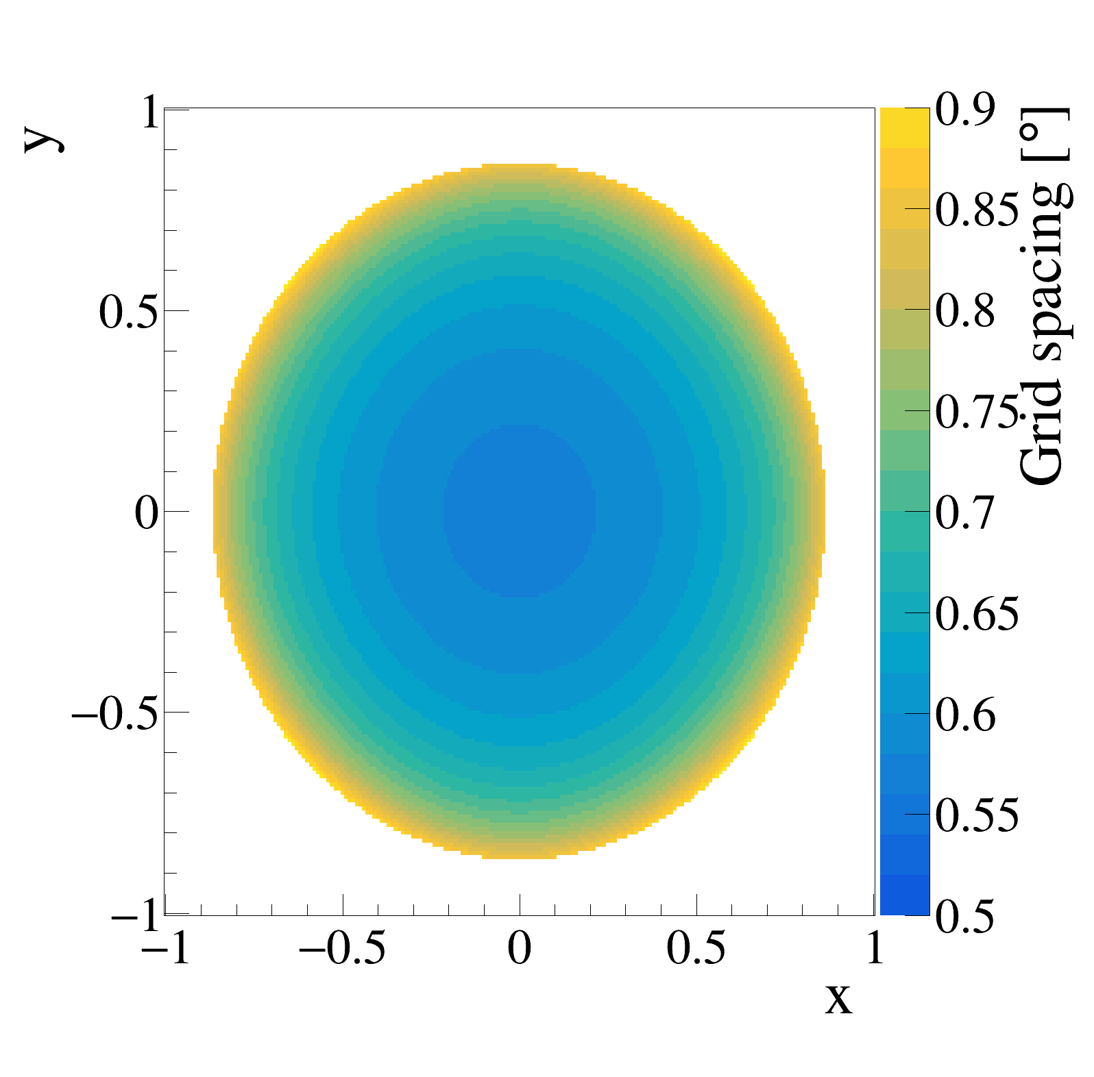
Figure 6: Grid spacing (in degrees) as a function of sky position. The outer circle in figure corresponds to the edge of FOV (120^∘) and the centre marks position of on-axis photons.

To make the database, steps given in Algorithm A are used. The use of a very bright GRB (200 ph/cm²) minimises statistical fluctuations in the database (and thereby in the mapping function). The spectrum is flat (equal flux) across all energies to enable spectral corrections as described in Section 4.3. The effect of these fixed values (of spectrum and fluence) used to generate the reference database is discussed further in Section 5.1. To scale for the source flux, the database stores fractional counts as shown in Eqn. (3), where the terms are as defined in Algorithm A.

$${\bar{m}_{i}(x,y)}=\frac{m_{i}(x,y)}{\sum\limits_{i}m_{i}(x,y)}$$ (3)

Algorithm A Database generation

1. Select a very bright GRB to generate the database. Fluence of 200 ph/cm². Flat spectrum.

2. Step $x$ from $-1$ to $1$ at a step size of $0.01$.

3. Step $y$ from $-1$ to $1$ at a step size of $0.01$.

4. If $x^{2}+y^{2}>1$, then reject that point.

5. Run Geant4 simulation for each combination $x,y$.

6. Store all event and hit information. This forms the extended database.

7. Store direction information along with original and deposited energies, of single-hit events only (with deposited energy $>50$ keV and $<$ 600 keV). This forms the reduced database.

8. Get the detected count map $m_{i}(x,y)$ (for all detector units $i$) and obtain the fractional counts ${\bar{m}_{i}(x,y)}$ as given in Eqn.(3). Store ${\bar{m}_{i}(x,y)}$ for all positions ($x,y$) to form the truncated database.

The entire extended database (including details of all hits and events) takes $\sim$ 1.2 Terabytes of disk space, while the reduced database (with details of single-hit events and necessary ancillary information) takes $\sim$ 80 Gigabytes space. The thresholds used for single-hit event selection (see Algorithm A) in the reduced database are chosen to reduce counts from the diffuse background. While a truncated database with just ${\bar{m}_{i}(x,y)}$ values (500 Megabytes) can also be used, this does not allow for GRB spectral corrections.

4.2 Routine-I : Modulation curve

The modulation curve method maps the counts in the outermost detector units to source position using an empirical relation composed of two sinusoidal components with 180^∘ and 360^∘ periodicities (see Eqn. (4)). The outermost detector units (consisting of GAGG units on the periphery of the entire detector array) are used as their position makes the detected counts sensitive to source position. The 180^∘ component arises because the GAGG units are shaped like rectangular slabs, where some units have their long edge facing the GRB direction and other units (placed 90^∘ away) have the short edge facing the source direction. Thus the detected counts are modulated in proportion to the geometrical cross section of the GAGG units as seen by the GRB. The 360^∘ component arises because only one side of the GAGG walls (the outer side) is covered by a multi-layered shield which reduces counts for a source placed on that side. Thus, GAGG units placed on the opposite side of the detector array as seen from the GRB will have higher counts than GAGG units placed closer to the source. The sum of these two components describes the count modulation in the periphery units.

The phase ($p_{1}$ and $p_{4}$) of the modulation in Eqn. (4) can be used to determine the azimuthal angle ($\alpha$), while the amplitude ($p_{0}$ and $p_{3}$) can be used to determine the zenith angle ($\delta$). The mapping makes use of detector angle $\phi_{d}$, defined as the angle subtended by the centre of each detector unit, at the centre of the local hexagonal (see Fig. 1(a)). The steps involved in implementing this routine are specified in Algorithm I.

$$f(\phi_{d})=p_{2}+p_{0}\cdot cos(2(\phi_{d}+p_{1}))+p_{3}\cdot cos(\phi_{d}+p_{4}),$$ (4)

Algorithm I Modulation curve

1. Compute $\phi_{d}$ for all detectors on the periphery. This gives 24 possible angles (bins) for 72 detector units (such that 3 detector units have the same angle $\phi_{d}$).

2. Average the counts of the 3 units per angular bin. Plot averaged counts against the angle $\phi_{d}$.

3. Fit Eqn.(4) to the detected counts and obtain parameters $p_{0}$ to $p_{4}$. To weight the fit, use the propagated error obtained from Poisson variances in counts of each detector unit (see Fig. 7).

4. Use relation in Eqn.(5) to estimate ${\hat{\alpha}}$.

5. Find $a_{m}$ using $\hat{\alpha}$. Use Eqn.(6) to estimate $\hat{\delta}$.

6. Propagate errors on the fit parameters to obtain the uncertainty ($\sigma_{\alpha},\sigma_{\delta}$) on estimated values.

$${\hat{\alpha}} =\begin{cases}p_{4}-\pi\,;\mathrm{Case\,I}\\ p_{1}\,;\mathrm{Case\,II}\end{cases}$$ (5)

$${\hat{\delta}} =\cos^{-1}\left(\frac{p_{0}}{a_{m}}\right)$$ (6)

Figure 7: Example modulation curve of outermost detectors (for $\alpha=-63^{\circ},\delta=48^{\circ}$) fit by Eqn. (4)

The relationship between parameters ($p_{0}$ to $p_{4}$) and sky position ($\delta$,$\alpha$) is obtained by searching for correlations in randomly simulated GRBs at different sky positions. It is seen that the phase of both 360^∘ ($p_{4}$) and 180^∘ ($p_{1}$) components correlate well with the azimuthal angle ($\alpha$). This correlation is independent of zenith angle ($\delta$) and the source spectrum. The 360^∘ component maps increased counts with detector units opposite to the azimuthal direction of the source. The 180^∘ component maps increased counts on both the detector units facing the GRB as well as on detector units placed diametrically opposite. Thus the phase angles $p_{1}$ and $p_{4}$ have similar values and either of these can be used to find $\alpha$. However, for some source positions (at low $\delta$ values) the 180^∘ component maps these modulations better (as the amplitude of the 360^∘ is smaller than the 180^∘ for small $\delta$). Thus, the preferred way to obtain $\hat{\alpha}$ is to use $p_{4}$ directly when $p_{1}$ and $p_{4}$ match (Case I). When they do not match (Case II), the phase angle indicated by $p_{1}$ is used.

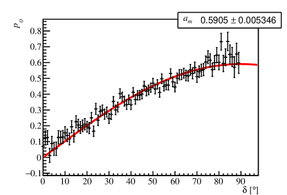
Figure 8: Relation between angle ($\delta$) and amplitude $p_{0}$ (see Eqn. (6))

As mentioned before, the amplitude of the 360^∘ component is sensitive to the zenith angle. This is because the modulation will be minimum (ideally zero) when the source is at the zenith (all units are equally illuminated) and maximum when the source is near the horizon (units facing the source are maximally illuminated). Fig. 8 shows this relation between $\delta$ and amplitude $p_{0}$ as obtained from the simulations. The sinusoidal relation, with parameter $a_{m}$, is quantified by Eqn. (6). The expression has a weak dependence on $\alpha$ (since $a_{m}$ changes slightly with $\alpha$). Thus, a two-step solution is needed to find the source location. Values of $a_{m}$ for different $\alpha$ are pre-computed using simulations and are seen to vary by less than 10%.

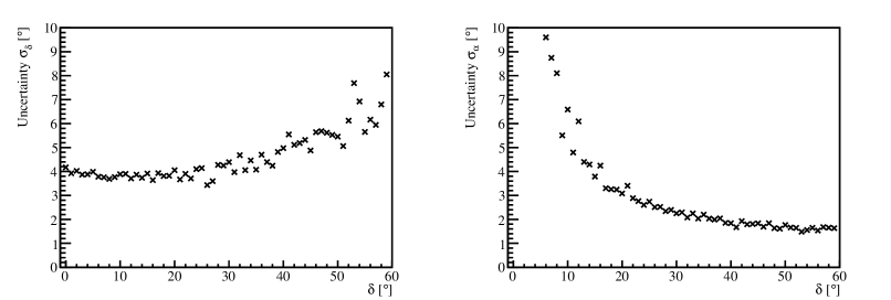
(a)                                                                           (b)

Figure 9: Uncertainties (a) $\sigma_{\delta}$ and (b) $\sigma_{\alpha}$ as a function of zenith angle ($\delta$) for the modulation curve routine. The values are plotted till ${\delta}=60^{\circ}$ (edge of FOV) for a GRB of median fluence.

$\sigma_{\delta}$ and $\sigma_{\alpha}$ are evaluated for different parameters as specified in Table 1 (see Fig. 9). For large $\delta$, $\sigma_{\delta}$ increases due to low counts in many detector units. At small $\delta$, the position angle $\alpha$ is not very well defined, thereby leading to larger $\sigma_{\alpha}$. As seen in following sections, these trends are true irrespective of the localisation routine used. The important result worth noting is that ${\sigma_{\delta}}\lesssim 8^{\circ}$ at all positions within the FOV (for a median fluence GRB).

4.3 Routine-II - Minimisation of $\chi^{2}$

The minimisation of Pearson’s $\chi^{2}$ is a classic routine used by Fermi GBM(Connaughton et al., 2015), CGRO BATSE (Pendleton et al., 1999), POLAR (Suarez-Garcia et al., 2010), AstroSat CZTI (Bhalerao et al., 2017), SSM (Ramadevi et al., 2017) and many other indirect imaging missions. The mapping function is obtained numerically and makes use of a pre-computed database. The inversion is done by comparing the measured counts ($c$) with the database modeled counts ($m$) using the $\chi^{2}$ statistic (Eqn. (7)). This statistic is computed for each position in the simulated database and the location of the minimum of the statistic is chosen as the best estimate of the source position.

$$\chi^{2}(x,y)=\sum_{i=1}\frac{(c_{i}-c_{tot}\cdot{\bar{m}_{i}(x,y)})^{2}}{c_{tot}\cdot{\bar{m}_{i}(x,y)}},$$ (7)

where, $c_{i}$ is the measured counts in detector unit $i$, $c_{tot}=\sum c_{i}$ is total number of counts in the count map, and ${\bar{m}_{i}(x,y)}$ the fractional database counts. The estimation of uncertainties is based on the $\chi^{2}$ density distribution for binned count data, which in turn uses the assumption of Gaussian distributed data in each detector unit (bin). The steps used to implement this routine are given in Algorithm II.

Algorithm II $\chi^{2}$ routine

1. Obtain spectrum of the GRB. Get corrected database count for this spectrum using Eqn.(8).

2. Compare detected count map with database using Eqn.(7).

3. Chose position with a minimum $\chi^{2}(x,y)$ value ($\chi^{2}_{min}$) as source position $(x_{min},y_{min})$.

4. Estimate $\hat{\delta}$ and $\hat{\alpha}$ using position of minimum and co-ordinate transformation ($x_{min},y_{min}~{}\mapsto~{}{\hat{\delta},\hat{\alpha}}$).

5. Get variation of $\chi^{2}$ with $x$ (at $y=y_{min}$) around minimum. Fit this with a parabola. Find $x_{1}$ and $x_{2}$ at which the parabola intersects $\chi^{2}=\chi^{2}_{min}+1$. Get $\sigma_{x}=0.5(x_{1}-x_{2})$

6. Repeat procedure to get $\sigma_{y}$.

7. Find $\sigma_{\delta}$ and $\sigma_{\alpha}$ using $\sigma_{x},\sigma_{y}$ and error propagation (from Cartesian to spherical co-ordinates).

The counts $m_{i}$ are corrected for spectral shape using Eqn.(8). These corrected $m^{\prime}_{i}$ are then used to get the fractional counts ${\bar{m}_{i}}$. Correction for the source spectrum is done by dividing the SPHiNX energy range into 5 keV bands. In Eqn.(8), $m_{ij}$ is the detected counts in the $j$-th (5 keV) energy bin for detector unit $i$ and $k_{j}$ is the spectral flux in the $j$-th band. $N^{uni}$ is the number of integrated photons across the flat spectrum (used to generate the database) and $N^{GRB}$ denotes the integrated photons across the actual GRB spectrum. In order to perform this correction, the database needs to store energy information of each simulated hit. This makes the database relatively large in size. The correction in Eqn.(8) assumes that counts in a particular band are only affected by photons in that band. This ignores the detector response which will lead to an additional systematic uncertainty as discussed in Section 5.

$$m^{\prime}_{i}=\frac{N^{uni}}{N^{GRB}}\sum_{j}\left(m_{ij}\cdot\frac{k_{j}^{GRB}}{k_{j}^{uni}}\right).$$ (8)

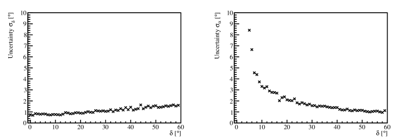
(a)                                                                           (b)

Figure 10: Uncertainty (a) $\sigma_{\delta}$ and (b) $\sigma_{\alpha}$ for $\chi^{2}$ routine as a function of $\delta$.

Fig. 10 shows the obtained uncertainties as a function of source position $\delta$ for this routine (for a median fluence GRB). As seen, the obtained uncertainties are much lower than those for the modulation curve routine. The trends though, remain the same as Routine-I : $\sigma_{\delta}$ increases with $\delta$ and $\sigma_{\alpha}$ has very high values for low $\delta$.

Instead of looking at uncertainties on two separate parameters, it is convenient to express localisation uncertainty in terms of the error radius. The error radius is defined in terms of the half angle of a cone which subtends the same solid angle on the sky as the uncertainty region defined by $\sigma_{\delta}$ and $\sigma_{\alpha}$. This means that the error radius is well defined even when the azimuthal angle ($\alpha$) is undefined near zenith. For small uncertainties, $\sigma_{\delta}$ and $\sigma_{\alpha}$ can be converted to the error radius ($\psi$) using

$$2\pi\cdot\big{(}1-{\cos(\psi)}\big{)}\approx{4\cdot\sigma_{\delta}}\cdot{\sigma_{\alpha}}\cdot\sin{{(\hat{\delta})}}$$ (9)

Fig. 11 shows the error radius for the $\chi^{2}$ routine at different positions on the sky. The error radius increases towards the edge of the FOV and is less than $\sim 1^{\circ}$ for most of the FOV. While the obtained uncertainties are very low, these values do not account for systematics and background effects, which are discussed further in Section 5.

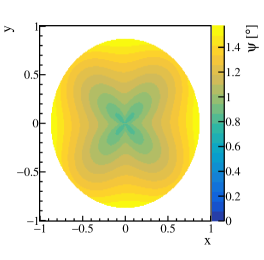
Figure 11: Error radius as a function of sky position. Figure obtained using Eqn. (9) with $\sigma_{\alpha},\sigma_{\delta}$ obtained at positions listed in Table 1.

The error radius can also be directly obtained using two-dimensional contours on the $\chi^{2}$ value. However, the grid-spacing used is often too sparse to get smooth contours as discussed in Section 5. The simpler procedure of using parabolic fits is therefore preferred for the $\chi^{2}$ routine.

4.4 Routine-III : Maximising the likelihood

The implementation and details of the likelihood routine are very similar to the $\chi^{2}$ routine. The differences arise in the method used to get the best estimate, in the calculation of uncertainties and in the use of a prior. The steps used to implement the likelihood routine are given in Algorithm III. The $\chi^{2}$ routine provides a convenient approach for performing the inversion in the limit of Gaussian distributed data, which holds true when sufficiently high ($\gtrsim 20$) counts are present in all detector units. This is indeed true for many GRBs (with fluence above median GRBs). For the other GRBs a more accurate routine involves computing the Poisson based likelihood function and maximising this likelihood for obtaining the inversion.

Algorithm III Likelihood Routine

1. Correct database counts for the GRB spectrum (Eqn. (8)).

2. Compute 2D posterior probability in $(x,y)$ with a uniform prior for GRBs in the sky using Eqn. (11).

   1. For each point $(x,y)$ in sky compute likelihood that detector units $i$ will observe the counts $m_{i}(x,y)$ and find its logarithm. Add the log-likelihoods for all detector units $i$ to find total log-likelihood.

   2. Take the exponential of the total log-likelihood and multiply it with the prior $\left(\sqrt{\frac{x^{2}+y^{2}}{R^{2}}}\right)$

3. Make a regular grid in $(\delta,\alpha)$. Linearly interpolate on the database grid to find posteriors for all the points on the new grid.

4. Obtain one-dimensional posterior probability distributions over $\delta$ and $\alpha$ separately by marginalising this two-dimensional distribution.

5. Obtain an estimate of the source position ($\hat{\delta},\hat{\alpha}$) using the MAP (maximum a posteriori estimate) with uncertainties ($\sigma_{\delta},\sigma_{\alpha}$) computed using the 68% confidence interval around the MAP estimate.

The Poisson based likelihood function, which relates the measured counts $m$ to the database modeled counts $c$, is easily computed using the expression for the Poisson distribution as

$$L(c_{i}|{\delta,\alpha})=\prod_{i}\frac{m_{i}({\delta,\alpha})^{c_{i}}}{c_{i}!}e^{{-m_{i}(\delta,\alpha)}}$$ (10)

Using Bayesian inference and a uniform prior for distribution of GRBs in the sky gives the posterior probability distribution $p(x,y|c_{i})$ as

$$\begin{split}p(x,y|c_{i})\propto\prod_{i}\left\{\frac{\big{(}c_{tot}\cdot{\bar{m}_{i}(x,y)}\big{)}^{c_{i}}}{c_{i}!}\exp\big{(}-c_{tot}\cdot{\bar{m}_{i}(x,y)}\big{)}\right\}\\ \cdot\left(\sqrt{\frac{x^{2}+y^{2}}{R^{2}}}\right)\end{split}$$ (11)

In this routine, the likelihood is computed for all points in the database. However, to estimate uncertainties, more points are needed as the marginalised posterior will often be confined to one or two grid-intervals of the database. A linear 2D interpolation of the posterior probability is done over a regular grid in $\delta,\alpha$ for ease of obtaining marginalised posteriors. A typical posterior distribution for a median fluence GRB obtained using a finely gridded database (grid-size 0.001 in $x,y$) and linear interpolation (to a 0.05^∘ regular grid in $\delta,\alpha$) is shown in Fig. 12.

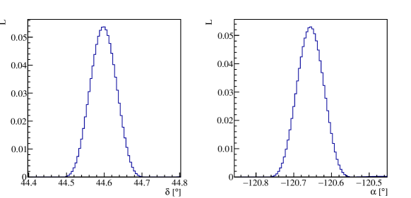
(a)                                         (b)

Figure 12: Marginalised posterior in (a) $\delta$ and (b) $\alpha$ for the likelihood routine (for a median fluence GRB)

The figure shows that uncertainties in the likelihood routine can be as low as $\sim 0.2^{\circ}$ if a finely gridded database is used. Typically systematic errors (Section 5.1) will be much larger than this and will dominate the localisation uncertainty .

5 Summary and Discussions

The results obtained demonstrate the ability of the SPHiNX design to localise GRBs. The effect of systematics like the presence of background and the use of a gridded database generated via Monte-Carlo simulations is considered below.

5.1 Systematics and Background effects

There are a number of additional sources of uncertainty in localisation, which arise from the design and characteristics of the detectors used and from approximations used to implement each routine. The most important ones which dominate the uncertainty on localisation are listed below.

5.1.1 Detector effects (efficiency and energy resolution)

The routines assume that all detector units have equal efficiency for photon detection. Calibration of the relative efficiencies of all detector units would be required to renormalise the obtained counts. Any uncertainty in the detector efficiency calibration will propagate to uncertainty in source position.

The two database routines use spectral corrections as given in Eqn. (8). The spectral correction depends on the knowledge of the source spectrum, which in turn depends on the spectral response. GAGG units with a better energy resolution (than plastic) of $\sim$24% at 60 keV have the potential to give a reconstructed spectrum comparable with Fermi GBM. Once the spectral response is known, it can be incorporated into the spectral correction of Eqn. (8). Calibration uncertainties in the spectral response will affect source localisation. An associated fact is that the spectral response of detector units will have a weak dependence on source position. Although rigorous techniques exist, which solve for the source spectrum and position simultaneously (Burgess et al., 2018), a simpler iterative approach for calibrating both the spectral response and the derived localisation is also possible.

These systematic uncertainties caused by imperfections in detector calibration, will be estimated post detector assembly by benchmarking simulations against calibration measurements as done in Chauvin et al. (2017); Yonetoku et al. (2011).

5.1.2 Background

Background count rates during a GRB should be constant given the relatively short duration of each GRB. Thus measurement of the background rates before and after the GRB event enables its modeling and subtraction and the localisation estimates ($\hat{\delta},\hat{\alpha}$) will remain unaffected. The background measurement though, will have measurement errors. This will propagate through the routines to increase uncertainty on source position. The background uncertainty is incorporated into each routine by simulating the expected background as given in Xie & Pearce (2018). The expected background rate for localisation events (single-hits above 50 keV) is $\sim 760$ cts/s across the entire detector array.

If $b_{T}$ is the total background counts measured in total time $t_{b}$ and $t_{s}$ is the time duration of the GRB, then the expected number of background counts $b_{m}$ during the GRB is simply

$$b_{m}=b_{T}\cdot\frac{t_{s}}{t_{b}}\equiv r\cdot{b_{T}}$$ (12)

Generally $r$ is less than unity as the window $t_{b}$ is made large enough to minimise uncertainty and measure a stable background rate. Let ${n=s+b}$ are the total detected counts, where ${s}$ gives the source (GRB) counts and $b$ the background counts. For the modulation curve routine, this simply increases the uncertainty on counts in each outermost detector unit. The new uncertainties on each angular bin ($\phi_{d}$) will be

$$\sqrt{{s_{i}}+b_{i}(1+r)},$$

(instead of $\sqrt{{s_{i}}}$), where $b_{i}$ is the expected background ($b_{m}$) in each detector unit $i$. The associated increase in $\sigma_{\alpha},\sigma_{\delta}$ is found by fitting Eqn. (4) to this data with higher uncertainties.

The $\chi^{2}$ expression of Eqn. (7) can be modified to similarly account for the background uncertainty as

$$\chi^{2}(x,y)=\sum_{i}\frac{(c_{i}-c_{tot}\cdot{\bar{m}_{i}(x,y)})^{2}}{c_{tot}\cdot{\bar{m}_{i}(x,y)}+b_{i}(1+r)}$$ (13)

The likelihood expression can also be modified to give Eqn. (14), where ${n_{mi}}=c_{tot}\cdot{\bar{m}}_{i}(x,y)+b_{i}$ is and $b_{Ti}$ is the measured background (in time $t_{b}$) in detector unit $i$.

$$p(x,y|c_{i})\propto\prod_{i}\left\{\frac{\exp{-({n_{mi}}+b_{Ti})}}{r}\sum_{j=0}^{\infty}\left(\frac{{n_{mi}}^{{s_{i}}+j}\,b_{Ti}^{j/r}}{({s_{i}}+j)!(j/r)!}\right)\right\}$$ (14)

$$\cdot\left(\sqrt{\frac{x^{2}+y^{2}}{R^{2}}}\right)$$

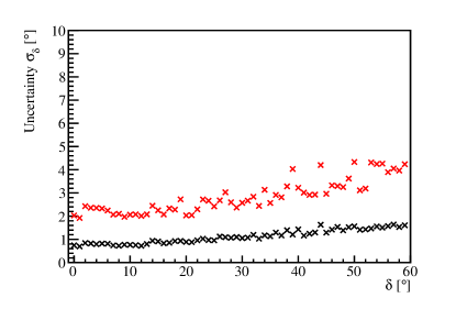
Figure 13: Increase in uncertainty due to background uncertainties (measured for 300s) in the $\chi^{2}$ routine for a median fluence GRB lasting 23s . Black points are before background correction and red points are after background correction.

The result of implementing these corrections is shown in Fig. 13 for the $\chi^{2}$ routine. As seen from the figure, background measurement uncertainties (for $t_{b}$ = 300s, $t_{s}$ = 20s) increase the localisation uncertainty by $\sim 2^{\circ}$ (for a GRB with median fluence). These uncertainties are expected to reduce as the orbital background measurement improves ($t_{b}$ increases). This treatment assumes a constant background during the time window of measurement. The background rates may vary during a GRB event. This can be treated by interpolating between the measured rates before and after the GRB. In such cases, the uncertainty on the background will be derived from the uncertainty of the interpolation parameters, which will be Gaussian (and not Poisson) distributed. The localisation uncertainty in such a case can be handled by re-writing the likelihood term as done in case of PGSTAT in Xspec .

5.1.3 Use of the database

Some of the assumptions used to create the database give rise to systematic offsets (measured as the angular distances $\partial_{\delta},\partial_{\alpha}$ between the actual and estimated source positions). This is shown in Fig. 14 for the $\chi^{2}$ database routines. The simulated database is made with a fluence of 200 ph/cm² and lowering this to 20 ph/cm² increases the average offsets from $1.5^{\circ}$ to $3.5^{\circ}$. This shows that the use of Monte-Carlo techniques involved in creating the database introduces an additional source of uncertainty due to Poisson fluctuations in the database counts. As average offsets of $\sim 1.5^{\circ}$ do not affect polarisation measurements adversely (see Fig. 3), the database (with 200 ph/cm²) is used by default.

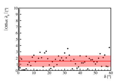
Figure 14: Systematic offsets ($\partial_{\delta}$) in the $\chi^{2}$ routine. The mean and $1\sigma$ deviation for offsets are highlighted.

For the routines using the database, interpolation enables estimation of uncertainty in between the non-regularly spaced grid points on the sky. Contour-based non-interpolative methods can only be used for GRBs with low fluence as in such cases (see next section) the uncertainty is much greater than the grid-size, thereby allowing construction of smooth contours. This is seen in Fig. 15 for a GRB with very weak fluence.

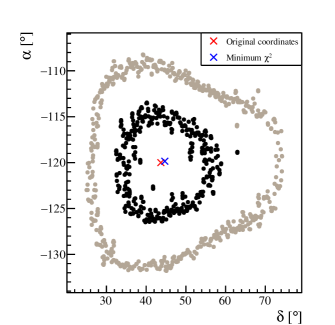
Figure 15: Uncertainty contours (1$\sigma$ and 2$\sigma$) using the $\chi^{2}$ routine for a weak fluence GRB (2 ph/cm²).

The $\chi^{2}$ routine though, uses parabolic interpolation and standard error propagation to obtain uncertainty in sky co-ordinates. This causes the obtained localisation uncertainty to have a systematic azimuthal dependence (as seen in Fig. 11). The amplitude of this variation ($<1^{\circ}$) is much smaller than other systematic effects. The likelihood routine needs a smaller grid spacing to obtain posterior distributions and uncertainty estimates. One solution is to make an additional database in a small region of the sky (say $5^{\circ}\times 5^{\circ}$) with a finer grid size and increased fluence as discussed in Section 5.2.

5.1.4 GRB fluence effects

Photon counting statistics ensure that bright GRBs are better localised than faint GRBs. This is seen in Fig. 16 and is true irrespective of the routine used. SPHiNX can detect polarisation for GRBs with fluence $\gtrsim 20$ ph/cm² (Pearce et al., 2019). For these GRBs, the localisation uncertainty in $\delta$ using $\chi^{2}$ routine can be computed as

$$\sigma=\sqrt{{\sigma_{\delta}^{2}+\partial_{off}^{2}}+\sigma_{cal}^{2}},$$ (15)

where ${\sigma_{\delta}}<2.2^{\circ}$ is uncertainty including background and ${\partial_{off}}\sim 1.5^{\circ}$ is the average offset. If we take uncertainty due to calibration systematics to be $\sigma_{cal}\sim 2^{\circ}$, then for these GRBs $\sigma<3.4^{\circ}$ and the MDP does not increase significantly ($<5\%$) for all GRBs within the FOV (Fig. 3). SPHiNX can achieve a reasonable localisation (${\sigma_{\delta}}<5^{\circ}$) for weaker GRBs too (with fluence $>$10 ph/cm²).

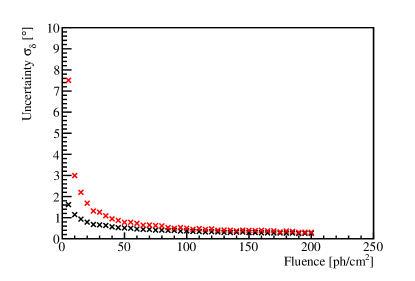
Figure 16: Uncertainty $\sigma_{\delta}$ for the $\chi^{2}$ routine as a function of source fluence with (red) and without (black) background uncertainty ($t_{b}=$ 300s, $t_{s}=$ 20s).

5.2 Comparison of routines

The three routines considered in this paper are compared based on the assumptions, obtained uncertainty estimates, computational resources needed and possible use cases in Table 2. The computations were performed on one of the six cores of an Intel Xeon E5 CPU (assisted by 16 GBs of RAM space) and do not include time required for background correction. The database was stored on an external 3 Terabyte magnetic hard-disk connected via USB (which increases read times required to access the database).

Table 2: Comparison of Inversion routines

	Routine-I (Modulation)	Routine-II ($\chi^{2}$)	Routine-III (Likelihood)
Approximations	$\bullet$ Uses subset of detected counts.	$\bullet$ Uses all available counts.	$\bullet$ Uses all available counts.
	$\bullet$ Empirical expression as mapping function.	$\bullet$ Simulated database as mapping function.	$\bullet$ Simulated database as mapping function.
		$\bullet$ Gaussian approximation to Poisson distributed counts.	$\bullet$ Poisson distribution directly used.
		$\bullet$ Uncertainty estimate uses error propagation (assuming independent $\sigma_{x},\sigma_{y}$) and parabola fit around $\chi^{2}_{min}$.	$\bullet$ Uncertainty estimate uses linear interpolation and dependent on grid size of database.
Resources	$\bullet$ Fast one-step execution ($\sim$ 0.35 seconds).	$\bullet$ Slow execution (5 hours - spectral correction ; 35 sec - database read, minima search and uncertainty computation on standard grid).	$\bullet$ Slow execution (7 hours - creation of a fine-grid small region database, 5 hours - spectral correction ; 5 sec - database read, maxima search and uncertainty estimation on smaller database).
	$\bullet$ No need for a database. Additional storage and read / write to hard-disk not required.	$\bullet$ Additional storage for an external database necessary.	$\bullet$ Additional finely gridded database ($\sim 7$ Gigabytes) necessary for obtaining uncertainty.
Uncertainty	$\bullet$ Large localisation uncertainty. ${\sigma_{\delta}}~{}\simeq~{}4^{\circ}$ without offset and background correction.	$\bullet$ Low uncertainty. ${\sigma_{\delta}}\simeq 1^{\circ}$ without offset and background correction.	$\bullet$ Low uncertainty. ${\sigma_{\delta}}\sim 0.2^{\circ}$ without offset and background correction.
Possible use	$\bullet$ Quick estimates for light-weight on-board computation. $\bullet$ First level estimate used to reduce and refine search space for a fine grid Likelihood based localisation.	$\bullet$ Provides sufficiently accurate localisation to use with polarisation analysis.	$\bullet$ Can be combined with Routine-I for fine grid search over a small region to obtain very accurate localisation. Allows incorporation of a priori information.

6 Conclusion

This paper discusses three GRB localisation routines for use with the SPHiNX mission concept. On-board computation of localisation parameters is not foreseen in the current mission design due to the limited downlink cadence (of one downlink per day) which makes real-time localisation unfeasible. The main use of localisation will be to determine the source position offline for use with subsequent polarisation analysis.

Polarisation properties will not be significantly affected for a zenith angle uncertainty of ${\sigma_{\delta}}\lesssim 5^{\circ}$. For median fluence GRBs, the localisation uncertainty is mainly driven by the presence of systematic offsets and uncertainty in background measurements. For higher fluence GRBs, these uncertainties reduce considerably. Localisation will not be undertaken for GRBs with weaker fluence.

The modulation curve routine, with its light-weight implementation and independence from the GRB spectrum is suitable for quick computations. This routine has a higher localisation uncertainty as it does not utilise information from all detector units. However, it can be used to get a rough estimate of the source position which can in turn be used to make a finely gridded database over a small region. This finer database can then be used with the likelihood routine to obtain a more accurate localisation. This coarse but fast estimate can be used to issue GCN notices in future GRB mission proposals which have higher downlink cadence provided the mission design preserves the azimuthal symmetry needed for generating such modulation curves.

The $\chi^{2}$ routine is ideally suited for offline use with simple approximations to compute the uncertainty. This routine gives an estimate within the required accuracy for polarisation analysis. While better techniques (like the contour-based uncertainty estimate) can be used to improve accuracy, the likelihood based routine is preferred in such cases as it makes fewer assumptions.

The likelihood based routine makes the highest demand on use of computational resources (especially in the nested sum computation needed for background correction). It also needs a database with a finer grid-size. However, it provides more accurate positions (as it uses fewer assumptions). If source position accuracy is prioritised, then this method can be coupled to a database with higher fluence and smaller grid size (around the coarsely localised modulation routine estimate) to get an accurate position estimate. Such requirements may arise if SPHiNX localisations are needed for detailed follow up studies of a particular GRB.

More sophisticated routines based on neural networks or maximising other statistics (like the correlation between detected count map and database count map) can be also be used for localisation. It is unlikely though, that the accuracy will be significantly better than for the likelihood routine as the position accuracy is mainly limited by photon statistics and design / placement of the detectors. In general, localisation for Compton polarimeters can be improved if the placement and shielding of detector units can be carefully optimised (without compromising polarisation sensitivity) by using studies similar to the ones done for coded aperture masks (Fenimore & Cannon, 1978).

About the authors

Lea Heckmann recently joined the MAGIC group at the Max Planck Institute for Physics, Munich as a PhD student. She received her MSc degree in engineering physics from the Vienna University of Technology in 2018. The main part of her master thesis was conducted at KTH Royal Institute of Technology in Stockholm, focusing on simulation studies and data analysis for the SPHiNX mission.

Nirmal Iyer is currently a post-doctoral researcher working with the SPHiNX and X-Calibur projects at KTH Royal Institute of Technology, Stockholm. He received his PhD from Indian Institute of Science, Bangalore in 2016 for work with design and development of an X-ray sky monitor. He is interested in design and optimisation of X-ray detectors for astronomy.

Mózsi Kiss is working as a Researcher in Astroparticle Physics at KTH Royal Institute of Technology in Stockholm since 2011. He conducted his Master’s thesis work at the Stanford Linear Accelerator Center, US, working on Compton-based polarimetry in 2006, and received his Ph.D. from KTH Royal Institute of Technology in 2011 working on the construction and testing of the PoGO/PoGOLite balloon-borne Compton polarimeter. Current interests include detector construction, scientific ballooning, satellite-based payloads and X-ray/gamma-ray polarimetry.

Mark Pearce is professor of physics at KTH Royal Institute of Technology in Stockholm since 2007. He received a Ph.D. in 1996 from the University of Birmingham, UK, for research in experimental particle physics. He currently focusses on instrument development for X-/gamma-ray astrophysics and the study of compact astrophysical objects using X-ray polarimetry. He is Principal Investigator of the PoGO+ and SPHiNX missions for hard X-ray polarimetry and recently joined a related mission, X-Calibur. Since 2012, he is Head of the KTH Physics Department.

Fei Xie is a postdoc in INAF, Osservatorio Astronomico di Cagliari. She received her Ph.D. in astroparticle physics from the Institute of High Energy Physics, University of Chinese Academy of Sciences in 2016. After that, she joined the particle and astroparticle physics group in KTH Royal Institute of Technology and mainly focused on X-ray polarimetry, including background simulation, instrument optimisation. From the second half of 2018, she began to work on IXPE (Imaging X-ray Polarimetry Explorer) project in Italy.

References

- Abbott et al. (2017a) Abbott B. P., et al., 2017a, ApJ, 848, L12
- Abbott et al. (2017b) Abbott B. P., et al., 2017b, The Astrophysical Journal Letters, 848, L13
- Allison et al. (2016) Allison J., et al., 2016, Nucl. Instrum. Meth., A835, 186
- Antcheva et al. (2009) Antcheva I., et al., 2009, Computer Physics Communications, 180, 2499
- Barthelmy et al. (2005) Barthelmy S. D., et al., 2005, Space Sci. Rev., 120, 143
- Bhalerao et al. (2017) Bhalerao V., et al., 2017, Journal of Astrophysics and Astronomy, 38, 31
- Bhat et al. (2016) Bhat P. N., et al., 2016, The Astrophysical Journal Supplement Series, 223, 28
- Burgess et al. (2018) Burgess J. M., Yu H.-F., Greiner J., Mortlock D. J., 2018, MNRAS, 476, 1427
- Chauvin et al. (2017) Chauvin M., et al., 2017, Nuclear Instruments and Methods in Physics Research A, 859, 125
- Connaughton et al. (2015) Connaughton V., et al., 2015, ApJS, 216, 32
- Fenimore & Cannon (1978) Fenimore E. E., Cannon T. M., 1978, Appl. Opt., 17, 337
- Fishman et al. (1982) Fishman G. J., Meegan C. A., Parnell T. A., Wilson R. B., 1982, in Lingenfelter R. E., Hudson H. S., Worrall D. M., eds, American Institute of Physics Conference Series Vol. 77, Gamma Ray Transients and Related Astrophysical Phenomena. pp 443–451, doi:10.1063/1.33205
- Klebesadel et al. (1973) Klebesadel R. W., Strong I. B., Olson R. A., 1973, ApJ, 182, L85
- Kumar & Zhang (2015) Kumar P., Zhang B., 2015, Phys. Rep., 561, 1
- McConnell (2017) McConnell M., 2017, NEW ASTRONOMY REVIEWS, 76, 1–21
- Meegan et al. (2009) Meegan C., et al., 2009, ApJ, 702, 791
- Mészáros (2006) Mészáros P., 2006, Reports on Progress in Physics, 69, 2259
- Muleri (2014) Muleri F., 2014, ApJ, 782, 28
- Paciesas et al. (1999) Paciesas W. S., et al., 1999, ApJS, 122, 465
- Pearce et al. (2019) Pearce M., et al., 2019, Astropart. Phys., 104, 54
- Pendleton et al. (1999) Pendleton G. N., et al., 1999, ApJ, 512, 362
- Produit et al. (2005) Produit N., et al., 2005, Nuclear Instruments and Methods in Physics Research A, 550, 616
- Ramadevi et al. (2017) Ramadevi M. C., et al., 2017, Experimental Astronomy, 44, 11
- Suarez-Garcia et al. (2010) Suarez-Garcia E., et al., 2010, Nuclear Instruments and Methods in Physics Research A, 624, 624
- Toma et al. (2009) Toma K., et al., 2009, ApJ, 698, 1042
- Weisskopf et al. (2010) Weisskopf M. C., Elsner R. F., O’Dell S. L., 2010, in Space Telescopes and Instrumentation 2010: Ultraviolet to Gamma Ray. p. 77320E (arXiv:1006.3711), doi:10.1117/12.857357
- Xie & Pearce (2018) Xie F., Pearce M., 2018, Galaxies, 6, 50
- Yonetoku et al. (2011) Yonetoku D., et al., 2011, ApJ, 743, L30