Domain wall dynamics in the Landau–Lifshitz magnet
and the classical-quantum correspondence for spin transport

Abstract

We investigate the dynamics of spin in the axially anisotropic Landau–Lifshitz field theory with a magnetic domain wall initial condition. Employing the analytic scattering technique, we obtain the exact scattering data and reconstruct the time-evolved profile. We identify three qualitatively distinct regimes of spin transport, ranging from ballistic expansion in the easy-plane regime, absence of transport in the easy-axis regime and logarithmically enhanced diffusion for the isotropic interaction. Our results are in perfect qualitative agreement with those found in the anisotropic quantum Heisenberg spin-$1/2$ chain, indicating a remarkable classical-quantum correspondence for macroscopic spin transport.

Introduction.

The theory of exactly solvable partial differential equations Faddeev and Takhtajan (1987); Ablowitz and Clarkson (1991); Novikov et al. (1984); Drazin and Johnson (1989), colloquially known as the theory of solitons Zabusky and Kruskal (1965), represents one of the cornerstones of theoretical and mathematical physics. While the technique has been traditionally used mostly as a theoretical framework to describe various nonlinear wave phenomena such as dispersive shock waves Gurevich and Pitaevskii (1974); El and Hoefer (2016) and modulational instabilities Hasegawa (1984); Tracy et al. (1984); Ercolani et al. (1990), soliton systems also played an instrumental role in a broader range of physics applications, ranging from experimentally relevant setups with cold atoms and BECs Panayotis G. Kevrekidis and Dimitri J. Frantzeskakis and Ricardo Carretero-González (2008), ocean waves Osborne (2002), physics of plasmas and nonlinear media Heidemann et al. (2009), Josephson junctions and nonlinear optics Hasegawa and Kodama (1995); Malomed (2006); Chen et al. (2012), and many theoretical concepts including the AdS/CFT correspondence Minahan and Zarembo (2003); Kazakov et al. (2004), Gromov-Witten theory Marshakov (2008), Painlevé transcendents Fokas et al. (2006); Clarkson (2003); Gamayun et al. (2013) and random matrix theory Tracy and Widom (1994, 2011).

Exact results on the nonequilibrium properties of soliton systems, both near and far from equilibrium, are nonetheless extremely rare. This can attributed to the fact that, outside of a few exceptional cases Gamayun et al. (2015); Gamayun and Semenyakin (2016); Caudrelier and Doyon (2016); De Luca and Mussardo (2016), the formal integration scheme cannot be implemented in a fully analytic manner in general. For this reason, in physics application one mostly relies on linearization or various approximations Kivshar and Malomed (1989) and asymptotic techniques Ablowitz and Segur (1977); Deift and Zhou (1993); Deift et al. (1993). In this Letter, we identify an exceptional but physically relevant nonequilibrium scenario where the issue can be overcome. We consider the Landau–Lifshitz ferromagnet and calculate the exact nonlinear Fourier spectrum (scattering data) for the magnetic domain wall initial profile. This enables us to analytically explore its far-from-equilibrium transport properties. We study the time-evolution of the domain wall profile and separately treat three qualitatively different dynamical regimes. We conclude by comparing our findings with the analogous problem in the (integrable) quantum Heisenberg (anti)ferromagnet, and highlight a remarkable classical-quantum correspondence for the macroscopic spin transport.

Landau–Lifshitz model.

The Landau–Lifshitz model is a classical field theory which governs a precessional motion of spin field on the unit sphere, described by the equation of motion Lakshmanan et al. (1976); Lakshmanan (1977); Takhtajan (1977); Sklyanin (1979); Fogedby (1980); Faddeev and Takhtajan (1987)

$$\vec{S}_{t}=\vec{S}\times\vec{S}_{xx}+\vec{S}\times{\bf J}\,\vec{S},\qquad\vec{S}\cdot\vec{S}=1,$$ (1)

with $\vec{S}\equiv(S^{x},S^{y},S^{z})^{\rm T}$. Choosing the uniaxial anisotropy tensor ${\bf J}\equiv{\rm diag}(0,0,\delta)$, there are three regions to be distinguished by the value of the parameter $\varepsilon~{}\equiv~{}{\rm i}\sqrt{\delta}$: the easy-axis regime $\varepsilon^{2}<0$, the easy-plane regime $\varepsilon^{2}>0$, and the isotropic case $\varepsilon=0$. This model also appears in a long-wavelength description of the spinor Bose gases Lamacraft (2008); Kudo and Kawaguchi (2010).

Spin transport.

To study spin transport, we consider the initial profile in the form of a (smooth) domain wall of the width $x_{0}$,

$$\vec{S}(x,t=0)=\big{(}{\rm sech}{(x/x_{0})},0,\tanh{(x/x_{0})}\big{)}^{\rm T},$$ (2)

which connects two distinct (degenerate) vacua. With no loss of generality we can put $x_{0}=1$ by a simple rescaling $x\to x_{0}\,x$, $t\to x_{0}^{2}t$, $\varepsilon\to\varepsilon/x_{0}$.

To characterize spin dynamics, it is natural to use a dynamical quantity

$$m(t)=\int^{\infty}_{0}{\rm d}x\,\big{(}1-S^{z}(x,t)\big{)},$$ (3)

which measures the change of total magnetization in the right half-system and has been already employed in previous studies Ljubotina et al. (2017a); Misguich et al. (2017).

Eq. (1) is completely integrable and thus possesses infinitely many conserved charges. Spin density $S^{z}$ corresponds to the globally conserved Noether charge and should be distinguished from other charges (the momentum, energy, and higher charges) which are all initially localized at the domain boundary and undergo ballistic spreading, in exact analogy to the expansion of local conserved charges in the nonlinear Schrödinger equation Miao et al. (2019).

Nonlinear Fourier transform.

The standard procedure to integrate nonlinear integrable wave equations such as Eq. (1) is called the inverse scattering method. We briefly sketch the main relevant ideas below, while for the full description we refer to one of the standard textbooks Faddeev and Takhtajan (1987); Ablowitz and Clarkson (1991); Novikov et al. (1984).

Figure 1: Schematic representation of the integration protocol: the forward ‘nonlinear Fourier transform’ $\mathcal{F}$, maps the initial spin field $\vec{S}(x,0)$ to the spectral data $\{a(\lambda),b(\lambda)\}$. The latter satisfies simple time-evolution (8). The inverse transform $\mathcal{F}^{-1}$ amounts to solving an appropriate linear integral equation from where one reconstructs the time-evolved spin-field $\vec{S}(x,t)$.

The framework of integrability relies on a geometric picture of linear parallel transport for the auxiliary wavefunction $\psi=\psi(x,t)$,

$$\begin{split}\partial_{\sigma}\psi(\lambda;x,t)={\bf U}_{[\sigma]}(\lambda;x,t)\psi(\lambda;x,t),\end{split}$$ (4)

for $\sigma\in\{x,t\}$, and the spatial and temporal connection components are

$${\bf U}_{[x]}(\lambda) =\frac{1}{2{\rm i}}\sum_{\alpha}w_{\alpha}S^{\alpha}\boldsymbol{\sigma}^{\alpha},$$ (5)

$${\bf U}_{[t]}(\lambda) =\frac{1}{2{\rm i}}\sum_{\alpha}\!\left[w_{\alpha}(\vec{S}\times\vec{S}_{x})^{\alpha}\boldsymbol{\sigma}^{\alpha}\!-\!\frac{w_{x}w_{y}w_{z}}{w_{\alpha}}S^{\alpha}\boldsymbol{\sigma}^{\alpha}\right],$$ (6)

respectively Sklyanin (1979); Faddeev and Takhtajan (1987); Bikbaev et al. (2014). Here, $w_{x}=w_{y}=\sqrt{\lambda^{2}-\varepsilon^{2}}$, $w_{z}=\lambda$, and $\lambda$ is the spectral parameter on a two-sheeted Riemann surface $\mu(\lambda)=\sqrt{\lambda^{2}-\varepsilon^{2}}$. Eq. (1) follows from the zero-curvature condition $[\partial_{x}-{\bf U}_{[x]},\partial_{t}-{\bf U}_{[t]}]=0$, which is needed for the consistency of Eqs. (4). Imposing the initial condition (2), we construct two Jost solutions of the spatial part of Eqs. (4) ${\bf T}_{\pm}$, characterized by asymptotic behavior ${\bf T}_{+}(x\to\infty)=\exp{(\lambda x\boldsymbol{\sigma}^{z}/2{\rm i})}$ and ${\bf T}_{-}(x\to-\infty)=\exp{(-\lambda x\boldsymbol{\sigma}^{z}/2{\rm i})}{\rm i}\boldsymbol{\sigma}^{x}$. The transfer matrix ${\bf T}(\lambda;t)$ is defined as a unimodular constant matrix that interpolates between Jost solutions ${\bf T}_{-}={\bf T}_{+}{\bf T}(\lambda)$. It can be presented as

$${\bf T}(\lambda)=\begin{pmatrix}a(\lambda)&-\bar{b}(\lambda)\\ b(\lambda)&\bar{a}(\lambda)\end{pmatrix}.$$ (7)

Complex functions $a(\lambda)$ and $b(\lambda)$ are called scattering amplitudes and store full information about the initial profile. The scattering data satisfy simple time-evolution

$$a(\lambda,t)=a(\lambda,0),\quad b(\lambda,t)=b(\lambda,0)e^{{\rm i}(\lambda^{2}-\varepsilon^{2})t},$$ (8)

which can be inferred from the temporal part of Eqs. (4). The conserved charges can be expressed as moments of the ‘density of states’ $\rho(\lambda)=\log|a(\lambda)|^{2}$.

The solution to Eqs. (4) for the domain wall profile (2) leads to the following scattering data

$$a(\lambda,0) =\frac{\sqrt{\lambda^{2}-\varepsilon^{2}}\,\Gamma^{2}(\tfrac{1}{2}-\tfrac{{\rm i}}{2}\lambda)}{2\Gamma(1-\tfrac{{\rm i}}{2}(\lambda-\varepsilon))\Gamma(1-\tfrac{{\rm i}}{2}(\lambda+\varepsilon))},$$ (9)

$$b(\lambda,0) ={\rm i}\frac{\cosh{(\tfrac{\pi}{2}\varepsilon)}}{\cosh{(\tfrac{\pi}{2}\lambda)}}.$$ (10)

The time-evolution for the spin field can be restored from the scattering data (8) by the inverse transform, shown in Fig. 1. The latter takes the form of a linear integral Fredholm-type equation called the Gel’fand–Levitan–Marchenko (GLM) equation Faddeev and Takhtajan (1987). Its precise form depends crucially on the value $\varepsilon$ and the type of boundary condition adjoined to Eq. (1). The presented analysis is confined to the non-trivial topological sector of the theory which requires certain (sometimes subtle) adaptations of the standard procedure Gamayun et al. .

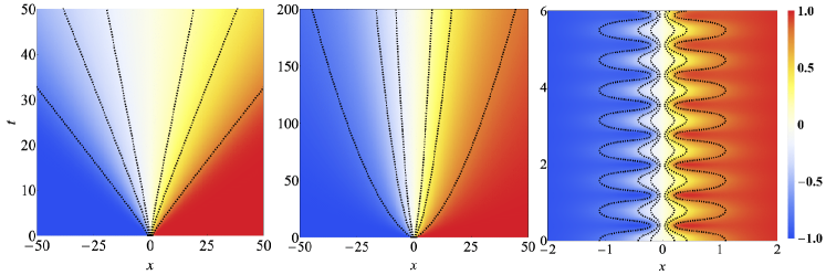
Figure 2: Time-dependent density profiles of $S^{z}$ component in the easy-plane $\delta=-1$ (left), isotropic $\delta=0$ (middle) and easy-axis $\delta=9$ (right) regimes, displaying ballistic spin transport, logarithmically enhanced diffusion and absence of transport, respectively. The dashed lines show $|S^{z}|~{}=~{}\{0.2,0.4,0.8\}$.

Easy-plane regime.

The absence of zeros of $a(\lambda)$ in the upper-half $\lambda$-plane for $\varepsilon\in\mathbb{R}$ means that the spectrum comprises only from a dispersive continuum of radiative modes. In fact, the origin of ballistic transport can be explained without recourse to the exact solution. It suffices to consider a hydrodynamic approximation to the equation of motion Whitham (1999). Introducing slow variables $S^{z}$ and $v\equiv-{\rm i}[\log S^{+}(x)]_{x}$, along with the nonlinearity $R\equiv[(S^{z}_{x}/\sqrt{1-(S^{z})^{2}})_{x}(1/\sqrt{1-(S^{z})^{2}})]_{x}$, Eq. (1) can be put in the form

$$S^{z}_{t}-[(1-(S^{z})^{2})v]_{x}=0,\quad v_{t}-[(\varepsilon^{2}-v^{2})S^{z}]_{x}=R.$$ (11)

By disregarding the nonlinearity term $R$, one has

$$\begin{pmatrix}S^{z}\\ v\end{pmatrix}_{t}=\begin{pmatrix}-2S^{z}v&1-(S^{z})^{2}\\ \varepsilon^{2}-v^{2}&-2S^{z}v\end{pmatrix}\begin{pmatrix}S^{z}\\ v\end{pmatrix}_{x}.$$ (12)

This WKB-type approximation can alternatively be viewed as the simplest case of a more general Whitham theory describing modulation of multiphase solutions to nonlinear wave equations Whitham (1999). The system (12) can be brought into the Riemann diagonal form $\partial_{t}r_{\pm}(x,t)+V_{\pm}(x,t)\partial_{x}r_{\pm}(x,t)=0$, with Riemann invariants $r_{\pm}=S^{z}v\pm\sqrt{(1-(S^{z})^{2})(\varepsilon^{2}-v^{2})}$, and characteristic velocities $V_{+}=r_{-}/2+3r_{+}/2$, $V_{-}=3r_{-}/2+r_{+}/2$.

The absence of scale in the initial profile motivates one to seek for the self-similar solution depending on the ray coordinate $\xi=x/t$, which yields the hydrodynamic equation $[V_{\pm}(\xi)-\xi]\partial_{\xi}r_{\pm}(\xi)=0$. To single out a unique solution, we need to additionally supply appropriate boundary conditions, which are set by the values $S^{z}(\xi_{\pm})=\pm 1$ and $v(\xi_{\pm})=v_{0}={\rm const}$ at $\xi_{\pm}$ – boundaries of the ballistically expanding region connecting two vacua. Inside this region the solution reads

$$S^{z}(\xi)=\frac{\xi}{2|\varepsilon|},\qquad v=|\varepsilon|=v_{0},\qquad\xi_{\pm}=\pm 2|\varepsilon|,$$ (13)

which implies linear growth of magnetization (3), namely $m(t)\simeq t\int^{2|\varepsilon|}_{0}{\rm d}\xi\,(1-S_{z}(\xi))=|\varepsilon|t$. Notice that the density of states $\rho(\lambda)$ develops a singularity at $\lambda_{*}=|\varepsilon|$, which thus defines a natural scale in the spectrum. The velocity of the hydrodynamic region is nothing but the velocity of the critical dispersive modes $v_{*}=2\lambda_{*}=|\xi_{\pm}|$. Moreover, a non-trivial solution on Euler scale exists only strictly in the easy-plane regime $\varepsilon^{2}>0$, whereas for $\varepsilon^{2}\leq 0$ the hydrodynamic solution trivializes, implying sub-ballistic transport.

Isotropic interaction.

For $\varepsilon=0$, the density of states $\rho(\lambda)$ logarithmically diverges at $\lambda\to 0$. As we demonstrate, this turns out to be an artefact of the specific domain-wall profile with perfectly anti-parallel asymptotic spin fields. For this reason, we also consider a deformed profile $\vec{S}=(\cos{\Phi},0,\sin{\Phi})^{\rm T}$, where $\Phi=(\gamma/\pi)\arcsin{(\tanh{x})}$ with the ‘twisting angle’ $\gamma\in[0,\pi)$. The induced correction to the scattering data for $\gamma\approx\pi$, computed with the first order perturbation theory, displaces the zero of $a(\lambda)$ at the origin, $a(0)\approx{\rm i}(\pi-\gamma)/2$, rendering the density of states finite.

At the isotropic point, there is a unique class of self-similar solutions to Eq. (1) which depend on the scaling variable $\zeta=x/\sqrt{t}$, governed by an ODE Lakshmanan et al. (1976),

$$-2\zeta\vec{S}_{\zeta}=\vec{S}\times\vec{S}_{\zeta\zeta},$$ (14)

which is usually studied in the context of the vortex filament dynamics Gutiérrez et al. (2003). For initial conditions with a jump discontinuity at the origin, Eq. (14) can be solved analytically. For large times, we observe that the twisted domain wall approaches the self-similar profile. The latter manifestly yields normal spin diffusion $m(t)\sim\mathfrak{D}(\gamma)\sqrt{t}$. The diffusion constant  $\mathfrak{D}(\gamma)$ plays a role of the filament curvature and can be approximated as $c\sqrt{E}$, with $c=\sqrt{2}(\pi-2\log(\sqrt{2}+1))\approx 2$ and $E=\vec{S}_{\zeta}^{2}$ being the conserved energy Gamayun and Lisovyy . Using relation $e^{-\pi E/2}=\cos(\gamma/2)$, one concludes that $\mathfrak{D}(\gamma)$ diverges as $\gamma\to\pi$, explaining the breakdown of normal diffusion for the untwisted profile (2). In order to quantify it, we have implemented an efficient numerical solver of the inverse (GLM) transform $\mathcal{F}^{-1}$ (see Fig. 1). Our data indicates a mild logarithmic (in time) divergence of $m(t)$ (see Fig. 3, inset plot), which nicely conforms with the type of singularity in the density of states. The twist of the boundary conditions removes the singularity and restores normal spin diffusion, as shown in Fig. 3.

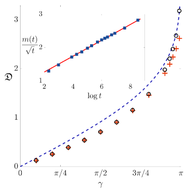
Figure 3: Spin diffusion constant $\mathfrak{D}(\gamma)$ as a function of the twisting angle $\gamma$, shown for the self-similarity solutions (open circles) and numerical integration up to $t=2000$ (red crosses). Blue dashed line shows the leading term in the large-$E$ asymptotic expansion of the self-similar solution. Inset: Numerical solution to the inverse scattering transform of the untwisted domain wall profile (2).

Easy-axis regime.

In distinction to the previous two regimes, the scattering data acquire an additional discrete component which physically corresponds to the (multi)soliton modes. The simplest among them are static (anti)-kink modes with topological charge $Q=\pm 1$, which coincide with domain wall (2) for $x_{0}=\pm 1/\sqrt{\delta}$. The kink persists in the spectrum for all $\delta>0$. Besides solitons, the spectrum involves a continuous spectrum of radiative modes, which, however, vanish for the the discrete set of ‘reflectionless anisotropies’ $\varepsilon={\rm i}(2n+1)$, $n\in\mathds{Z}$. The analyticity of $a(\lambda)$ can be restored with the uniformization map, $\lambda(z)=(z+\varepsilon^{2}z^{-1})/2$; soliton modes are then characterized by zeros of $a(z)$ located in the upper half $z$-plane. The spectrum of the domain wall does not involve any asymptotically free solitons, implying a trivial ballistic channel. The asymptotic scaling $m(t)\sim t^{0}$ is then a consequence of the finite difference between the domain wall profile and the stable kink. For instance, on the interval $0<\varepsilon<3{\rm i}$, the kink is the only soliton mode and thus the steady state of the domain wall dynamics. On the other hand, for larger values of anisotropy we obtained an infinite family of bound states which undergo periodic oscillatory motion. To our knowledge, such solutions have not been explicitly described previously in the literature Kosevich et al. (1990); Bogdan and Kovalev (1980); Svendsen and Fogedby (1993); Bikbaev et al. (2014), but similar ‘wobbling kinks’ have been already identified in the sine–Gordon model Segur (1983); De Rossi et al. (1998); G Kälbermann (2004); Ferreira et al. (2008). For example, for $n=1$ the scattering data read

$$a(z)={\rm i}\frac{(z-3{\rm i})(z^{2}-2{\rm i}z+9)}{(z+3{\rm i})(z^{2}+2{\rm i}z+9)},\quad b(z)=0,$$ (15)

and describes the kink-breather bound state which can be compactly parametrized by a complex stereographic angle $\varphi$,

$$S^{z}=\frac{1-|\varphi|^{2}}{1+|\varphi|^{2}},\qquad S^{x}+{\rm i}S^{y}=\frac{2\varphi}{1+|\varphi|^{2}},$$ (16)

reading

$$\varphi=\frac{e^{\eta_{0}}+e^{\eta_{+}}+2e^{\eta_{-}}}{1+2e^{\eta_{0}+\eta_{-}}+e^{\eta_{0}+\eta_{+}}}.$$ (17)

The phases $\eta_{i}(x,t)={\rm i}(k_{i}x+\omega_{i}t)$ and $k_{0}=-3{\rm i}$, $\omega_{0}=0$, and $k_{\pm}=\pm{\rm i}$ and $\omega_{\pm}=k^{2}_{\pm}-\varepsilon^{2}$ are determined from the scattering data (15). The full classification of the soliton spectrum is postponed to Gamayun et al. .

Classical-quantum correspondence.

The quantum integrable (lattice) counterpart to the equation of motion (1) is the celebrated anisotropic quantum Heisenberg spin chain $H~{}\simeq~{}-\sum_{i}\left(\hat{S}^{x}_{i}\hat{S}^{x}_{i+1}+\hat{S}^{y}_{i}\hat{S}^{y}_{i+1}+\Delta\hat{S}^{z}_{i}\hat{S}^{z}_{i+1}\right)$, the oldest known model solvable by the Bethe Ansatz Bethe (1931); Takahashi (1971); Gaudin (1971); Takahashi and Suzuki (1972). The time-evolution following a sharp magnetic domain and its dependence on anisotropy $\Delta$ has already been a subject of study in the past Gobert et al. (2005); Mossel and Caux (2010); Bertini et al. (2016); Collura et al. (2018); Ljubotina et al. (2017a); Misguich et al. (2017); Ljubotina et al. (2017b).

In the remainder of the Letter, we wish to elaborate on the perfect qualitative agreement in the spin dynamics of the classical and quantum anisotropic ferromagnets, in spite of rather discernible differences in the respective microscopic dynamics: the spectrum of excitations of quantum dynamics (classified in Takahashi (1971); Takahashi and Suzuki (1972)) consists of magnons (and bound states thereof) carrying a quantized amount of spin, whereas classical dynamics corresponds to the semi-classical long-wavelength spectrum of large spin-coherent states Sutherland (1995); Dhar and Sriram Shastry (2000); Kazakov et al. (2004); Bargheer et al. (2008).

To facilitate the comparisons, we briefly review the key known results. Ballistic expansion of the magnetic domain wall in the gapless regime $|\Delta|<1$ has been first computed numerically using the hydrodynamic theory for quantum integrable models Bertini et al. (2016) and latter obtained analytically in Collura et al. (2018). The dynamical freezing of the magnetic domain wall in the gapped regime $|\Delta|>1$ has been reported in Gobert et al. (2005); Ljubotina et al. (2017a); Misguich et al. (2017). In fact, the observed effect is once again a consequence of stable topological kink vacua, representing an inhomogeneous (infinite-volume) ground states with a finite spectral gap Alcaraz et al. (1995); Koma and Nachtergaele (1997) (which become unstable at $\Delta=1$). At the isotropic point, the observed logarithmically enhanced diffusion law in the isotropic Landau–Lifshitz model (cf. Fig. 3) appears to be compatible with the state-of-the-art numerical study Misguich et al. (2017) (which is missed, somehow, in Ljubotina et al. (2017b)). Curiously, the same type of correction has been found in the asymptotic behavior of the return probability amplitude for the domain wall initial state Stéphan (2017). Our twisted domain wall profile should be understood as a classical analogue of the tilted domain wall product states employed in Ljubotina et al. (2017b) which exhibit normal spin diffusion.

Although in this Letter we concentrated solely on the spin dynamics in the far-from-equilibrium regime (with a specific initial state), there exists a robust evidence that the classical-quantum correspondence holds also in thermal equilibrium in the conventional framework of linear response theory. The thermal spin diffusion constant (at half filling) in the lattice Landau–Lifshitz model – defined via the thermal average of the time-dependent auto-correlation $C(t)=\langle J(0)J(t)\rangle/L$ of the spin current $J(t)$ – has been numerically investigated in Prosen and Žunkovič (2013), where three distinct regimes have been identified: ballistic transport with a finite Drude weight $\mathcal{D}=\lim_{t\to\infty}C(t)$ in the easy-plane regime, normal diffusion with finite $D=\lim_{t\to\infty}\int^{t}_{0}C(t^{\prime}){\rm d}t^{\prime}$ in the easy-axis regime, and superdiffusion with a time-dependent diffusion constant $D(t)\sim t^{1/3}$ at the isotropic point. In the quantum Heisenberg spin-$1/2$ chain the picture remains qualitatively the same: in the easy-plane regime ($|\Delta|<1$), the finite spin Drude weight has been attributed to hidden quasi-local conservation laws Prosen and Ilievski (2013); Ilievski et al. (2016) and computed exactly in Ilievski and De Nardis (2017a, b) using the hydrodynamic theory for integrable models Castro-Alvaredo et al. (2016); Bertini et al. (2016). In the easy-axis regime ($|\Delta|>1$) one finds normal diffusion, theoretically explained in De Nardis et al. (2018a, b). Finally, the divergence of the spin diffusion constant at the isotropic point (at finite temperature and half filling) has been established in Ilievski et al. (2018). Numerical simulations Ljubotina et al. (2017a) provide a convincing evidence for super-diffusion with the Kardar-Parisi-Zhang (KPZ) dynamical exponent $\alpha=2/3$, later theoretically justified with the aid of a dimensional analysis in Gopalakrishnan and Vasseur (2018).

Conclusions.

We have studied the spin transport in the uniaxial Landau–Lifshitz ferromagnet initialized in the domain wall profile. We have computed the exact spectrum of nonlinear normal modes and expressed the time-evolved spin field as a solution of the inverse scattering transformation.

In the easy-plane regime we encountered ballistic expansion, which, to the leading order, can be captured by a simple hydrodynamic theory.

For the isotropic interaction, we rigorously established a divergent spin diffusion constant and explain the origin of the a modified diffusion law with a multiplicative logarithmic correction. The effect is shown to be a particularity of the initial state and can be regularized by a twist of the boundary conditions which restores normal diffusion. Such a ‘$\pi$-anomaly’ can be understood as an ‘infrared catastrophe’ due to a logarithmic divergence of the mode occupation function in the low-energy $\lambda\to 0$ limit.

In the easy-axis regime, the spectrum of the domain wall acquires non-trivial topologically charged (multi)soliton states which consists of breather modes superimposed on a kink. It remains an interesting open question whether wobbling kinks survive quantization, similar to the problem of quantum stability of cnoidal waves addressed in Bargheer et al. (2008). Analytic continuation into the easy-plane phase, $\varepsilon\to-{\rm i}\varepsilon$, can also be understood as destabilization of the kink mode into a dynamical domain wall.

Since the Landau–Lifshitz model can be regarded as a generic integrable $(1+1)$-dimensional soliton system, it is compelling to conjecture that the correspondence is a general feature of quantum integrable lattice models that admit a semi-classical limit (such as e.g. the sine–Gordon model, nonlinear sigma models, nonlinear Schrödinger equation, etc.). We hope that our results can stimulate further research in this direction. A separate interesting issue is whether similar correspondences appear even more broadly, e.g. in one of the non-integrable dynamical systems in higher dimensions.

Acknowledgments. We thank O. Lisovyy, J. De Nardis, M. Medenjak and T. Prosen for their comments. Y. M. and O. G. acknowledge the support from the European Research Council under ERC Advanced grant 743032 DYNAMINT. E. I. is supported by VENI grant number 680-47-454 by the Netherlands Organisation for Scientific Research (NWO).

References

- Faddeev and Takhtajan (1987) L. D. Faddeev and L. A. Takhtajan, Hamiltonian Methods in the Theory of Solitons (Springer Berlin Heidelberg, 1987).
- Ablowitz and Clarkson (1991) M. A. Ablowitz and P. A. Clarkson, Solitons, Nonlinear Evolution Equations and Inverse Scattering (Cambridge University Press, 1991).
- Novikov et al. (1984) S. Novikov, S. Manakov, L. Pitaevskii, and V. Zakharov, Theory of solitons: the inverse scattering method (Springer Science & Business Media, 1984).
- Drazin and Johnson (1989) P. G. Drazin and R. S. Johnson, Solitons (Cambridge University Press, 1989).
- Zabusky and Kruskal (1965) N. J. Zabusky and M. D. Kruskal, Phys. Rev. Lett. 15, 240 (1965).
- Gurevich and Pitaevskii (1974) A. Gurevich and L. Pitaevskii, J. Exp. Theor. Phys. 38, 291 (1974).
- El and Hoefer (2016) G. El and M. Hoefer, Phys. D 333, 11 (2016).
- Hasegawa (1984) A. Hasegawa, Opt. Lett. 9, 288 (1984).
- Tracy et al. (1984) E. R. Tracy, H. H. Chen, and Y. C. Lee, Phys. Rev. Lett. 53, 218 (1984).
- Ercolani et al. (1990) N. Ercolani, M. Forest, and D. W. McLaughlin, Phys. D 43, 349 (1990).
- Panayotis G. Kevrekidis and Dimitri J. Frantzeskakis and Ricardo Carretero-González (2008) Panayotis G. Kevrekidis and Dimitri J. Frantzeskakis and Ricardo Carretero-González, ed., Emergent Nonlinear Phenomena in Bose-Einstein Condensates (Springer Berlin Heidelberg, 2008).
- Osborne (2002) A. R. Osborne, in Scattering (Elsevier, 2002) pp. 637–666.
- Heidemann et al. (2009) R. Heidemann, S. Zhdanov, R. Sütterlin, H. M. Thomas, and G. E. Morfill, Phys. Rev. Lett. 102, 135002 (2009).
- Hasegawa and Kodama (1995) A. Hasegawa and Y. Kodama, Solitons in optical communications, 7 (Oxford University Press, 1995).
- Malomed (2006) B. A. Malomed, Soliton management in periodic systems (Springer Science & Business Media, 2006).
- Chen et al. (2012) Z. Chen, M. Segev, and D. N. Christodoulides, Rep. Prog. Phys. 75, 086401 (2012).
- Minahan and Zarembo (2003) J. A. Minahan and K. Zarembo, J. High Energy Phys. 2003, 013 (2003).
- Kazakov et al. (2004) V. A. Kazakov, A. Marshakov, J. A. Minahan, and K. Zarembo, J. High Energy Phys. 2004, 024 (2004).
- Marshakov (2008) A. Marshakov, J. High Energy Phys. 2008, 055 (2008).
- Fokas et al. (2006) A. Fokas, A. Its, A. Kapaev, and V. Novokshenov, Painlevé Transcendents (American Mathematical Society, 2006).
- Clarkson (2003) P. A. Clarkson, J. Comput. Appl. Math. 153, 127 (2003).
- Gamayun et al. (2013) O. Gamayun, N. Iorgov, and O. Lisovyy, J. Phys. A 46, 335203 (2013).
- Tracy and Widom (1994) C. A. Tracy and H. Widom, Commun. Math. Phys. 159, 151 (1994).
- Tracy and Widom (2011) C. Tracy and H. Widom, Publ. Res. Inst. Math. Sci. 47, 361 (2011).
- Gamayun et al. (2015) O. Gamayun, Y. V. Bezvershenko, and V. Cheianov, Phys. Rev. A 91, 031605 (2015).
- Gamayun and Semenyakin (2016) O. Gamayun and M. Semenyakin, J. Phys. A 49, 335201 (2016).
- Caudrelier and Doyon (2016) V. Caudrelier and B. Doyon, J. Phys. A 49, 445201 (2016).
- De Luca and Mussardo (2016) A. De Luca and G. Mussardo, J. Stat. Mech. Theory Exp. 2016, 064011 (2016).
- Kivshar and Malomed (1989) Y. S. Kivshar and B. A. Malomed, Rev. Mod. Phys. 61, 763 (1989).
- Ablowitz and Segur (1977) M. J. Ablowitz and H. Segur, Stud. Appl. Math. 57, 13 (1977).
- Deift and Zhou (1993) P. Deift and X. Zhou, Ann. Math. 137, 295 (1993).
- Deift et al. (1993) P. A. Deift, A. R. Its, and X. Zhou, in Springer Series in Nonlinear Dynamics (Springer Berlin Heidelberg, 1993) pp. 181–204.
- Lakshmanan et al. (1976) M. Lakshmanan, T. Ruijgrok, and C. Thompson, Phys. A 84, 577 (1976).
- Lakshmanan (1977) M. Lakshmanan, Phys. Lett. A 61, 53 (1977).
- Takhtajan (1977) L. Takhtajan, Phys. Lett. A 64, 235 (1977).
- Sklyanin (1979) E. K. Sklyanin, On complete integrability of the Landau-Lifshitz equation (1979).
- Fogedby (1980) H. C. Fogedby, J. Phys. A 13, 1467 (1980).
- Lamacraft (2008) A. Lamacraft, Phys. Rev. A 77, 063622 (2008).
- Kudo and Kawaguchi (2010) K. Kudo and Y. Kawaguchi, Phys. Rev. A 82, 053614 (2010).
- Ljubotina et al. (2017a) M. Ljubotina, M. Žnidarič, and T. Prosen, Nat. Commun. 8, 16117 (2017a).
- Misguich et al. (2017) G. Misguich, K. Mallick, and P. L. Krapivsky, Phys. Rev. B 96, 195151 (2017).
- Miao et al. (2019) Y. Miao, E. Ilievski, and O. Gamayun, Phys. Rev. A 99, 023605 (2019).
- Bikbaev et al. (2014) R. F. Bikbaev, A. I. Bobenko, and A. R. Its, Theor. Math. Phys. 178, 143 (2014).
- (44) O. Gamayun, E. Ilievski, and Y. Miao, In preparation.
- Whitham (1999) G. B. Whitham, Linear and Nonlinear Waves (John Wiley & Sons, Inc., 1999).
- Gutiérrez et al. (2003) S. Gutiérrez, J. Rivas, and L. Vega, Comm. Part. Differ. Equat. 28, 927 (2003).
- Note (1) This definition of the diffusions constant should not be confused with that of the Kubo linear response theory.
- (48) O. Gamayun and O. Lisovyy, arXiv preprint arXiv:1903.02105 .
- Kosevich et al. (1990) A. Kosevich, B. Ivanov, and A. Kovalev, Phys. Rep. 194, 117 (1990).
- Bogdan and Kovalev (1980) M. M. Bogdan and A. S. Kovalev, JETP Lett. 31, 424 (1980).
- Svendsen and Fogedby (1993) M. Svendsen and H. C. Fogedby, J. Phys. A 26, 1717 (1993).
- Segur (1983) H. Segur, J. Math. Phys. 24, 1439 (1983).
- De Rossi et al. (1998) A. De Rossi, C. Conti, and S. Trillo, Phys. Rev. Lett. 81, 85 (1998).
- G Kälbermann (2004) G Kälbermann, J. Phys. A 37, 11603 (2004).
- Ferreira et al. (2008) L. A. Ferreira, B. Piette, and W. J. Zakrzewski, Phys. Rev. E 77, 036613 (2008).
- Bethe (1931) H. Bethe, Z. Phys. 71, 205 (1931).
- Takahashi (1971) M. Takahashi, Prog. Theor. Phys. 46, 401 (1971).
- Gaudin (1971) M. Gaudin, Phys. Rev. Lett. 26, 1301 (1971).
- Takahashi and Suzuki (1972) M. Takahashi and M. Suzuki, Prog. Theor. Phys. 48, 2187 (1972).
- Gobert et al. (2005) D. Gobert, C. Kollath, U. Schollwöck, and G. Schütz, Phys. Rev. E 71, 036102 (2005).
- Mossel and Caux (2010) J. Mossel and J.-S. Caux, New J. Phys. 12, 055028 (2010).
- Bertini et al. (2016) B. Bertini, M. Collura, J. De Nardis, and M. Fagotti, Phys. Rev. Lett. 117, 207201 (2016).
- Collura et al. (2018) M. Collura, A. De Luca, and J. Viti, Phys. Rev. B 97, 081111 (2018).
- Ljubotina et al. (2017b) M. Ljubotina, M. Žnidarič, and T. Prosen, J. Phys. A 50, 475002 (2017b).
- Sutherland (1995) B. Sutherland, Phys. Rev. Lett. 74, 816 (1995).
- Dhar and Sriram Shastry (2000) A. Dhar and B. Sriram Shastry, Phys. Rev. Lett. 85, 2813 (2000).
- Bargheer et al. (2008) T. Bargheer, N. Beisert, and N. Gromov, New J. Phys. 10, 103023 (2008).
- Alcaraz et al. (1995) F. C. Alcaraz, S. R. Salinas, and W. F. Wreszinski, Phys. Rev. Lett. 75, 930 (1995).
- Koma and Nachtergaele (1997) T. Koma and B. Nachtergaele, Lett. Math. Phys. 40, 1 (1997).
- Stéphan (2017) J.-M. Stéphan, J. Stat. Mech. Theor. Exp. 2017, 103108 (2017).
- Prosen and Žunkovič (2013) T. Prosen and B. Žunkovič, Phys. Rev. Lett. 111, 040602 (2013).
- Prosen and Ilievski (2013) T. Prosen and E. Ilievski, Phys. Rev. Lett. 111, 057203 (2013).
- Ilievski et al. (2016) E. Ilievski, M. Medenjak, T. Prosen, and L. Zadnik, J. Stat. Mech. Theor. Exp. 2016, 064008 (2016).
- Ilievski and De Nardis (2017a) E. Ilievski and J. De Nardis, Phys. Rev. Lett. 119, 020602 (2017a).
- Ilievski and De Nardis (2017b) E. Ilievski and J. De Nardis, Phys. Rev. B 96, 081118 (2017b).
- Castro-Alvaredo et al. (2016) O. A. Castro-Alvaredo, B. Doyon, and T. Yoshimura, Phys. Rev. X 6, 041065 (2016).
- De Nardis et al. (2018a) J. De Nardis, D. Bernard, and B. Doyon, Phys. Rev. Lett. 121, 160603 (2018a).
- De Nardis et al. (2018b) J. De Nardis, D. Bernard, and B. Doyon, arXiv preprint arXiv:1812.00767 (2018b).
- Ilievski et al. (2018) E. Ilievski, J. De Nardis, M. Medenjak, and T. Prosen, Phys. Rev. Lett. 121, 230602 (2018).
- Gopalakrishnan and Vasseur (2018) S. Gopalakrishnan and R. Vasseur, arXiv preprint arXiv:1812.02701 (2018).