Active Anomaly Detection via Ensembles: Insights, Algorithms, and Interpretability

Abstract

Anomaly detection (AD) task corresponds to identifying the true anomalies from a given set of data instances. AD algorithms score the data instances and produce a ranked list of candidate anomalies, which are then analyzed by a human to discover the true anomalies. However, this process can be laborious for the human analyst when the number of false-positives is very high. Therefore, in many real-world AD applications including computer security and fraud prevention, the anomaly detector must be configurable by the human analyst to minimize the effort on false positives. One important way to configure the detector is by providing true labels (nominal or anomaly) for a few instances.

In this paper, we study the problem of active learning to automatically tune ensemble of anomaly detectors to maximize the number of true anomalies discovered. We make four main contributions towards this goal. First, we present an important insight that explains the practical successes of AD ensembles and how ensembles are naturally suited for active learning. This insight also allows us to relate the greedy query selection strategy to uncertainty sampling, with implications for label-efficient learning. Second, we present several algorithms for active learning with tree-based AD ensembles. A novel formalism called compact description (CD) is developed to describe the discovered anomalies. We propose algorithms based on the CD formalism to improve the diversity of discovered anomalies and to generate rule sets for improved interpretability of anomalous instances. To handle streaming data setting, we present a novel data drift detection algorithm that not only detects the drift robustly, but also allows us to take corrective actions to adapt the detector in a principled manner. Third, we present a novel algorithm called GLocalized Anomaly Detection (GLAD) for active learning with generic AD ensembles and an approach to generate succinct explanations from the resulting models. GLAD allows end-users to retain the use of simple and understandable global anomaly detectors by automatically learning their local relevance to specific data instances using label feedback. Fourth, we present extensive experiments to evaluate our insights and algorithms with tree-based AD ensembles in both batch and streaming settings. Our results show that in addition to discovering significantly more anomalies than state-of-the-art unsupervised baselines, our active learning algorithms under the streaming-data setup are competitive with the batch setup. Experiments using GLAD show its effectiveness in learning the local relevance of ensemble members to discover more anomalies when compared to baseline methods.

1 Introduction

We consider the problem of anomaly detection (AD), where the goal is to detect unusual but interesting data (referred to as anomalies) among the regular data (referred to as nominals). This problem has many real-world applications including credit card transactions, medical diagnostics, computer security, etc., where anomalies point to the presence of phenomena such as fraud, disease, malpractices, or novelty which could have a large impact on the domain, making their timely detection crucial.

Anomaly detection poses severe challenges that are not seen in traditional learning problems. First, anomalies are significantly fewer in number than nominal instances. Second, unlike classification problems, no hard decision boundary exists to separate anomalies and nominals. Instead, anomaly detection algorithms train models to compute scores for all instances, and report instances which receive the highest scores as anomalies. The candidate anomalies in the form of top-ranked data instances are analyzed by a human analyst to identify the true anomalies. Since most of the AD algorithms (?) only report technical outliers (i.e., data instances which do not fit a normal model as anomalies), the candidate set of anomalies may contain many false-positives, which will significantly increase the effort of human analyst in discovering true anomalies.

In this paper, we consider a human-in-the-loop learning framework for discovering anomalies via ensemble of detectors, where a human analyst provides label feedback (nominal or anomaly) for one or more data instances during each round of interaction. This feedback is used by the anomaly detector to change the scoring mechanism of data instances towards the goal of increasing the true anomalies appearing at the top of the ranked list. Our learning framework exploits the inherent strengths of ensembles for anomaly detection. Ensemble of anomaly detectors are shown to perform well in both unsupervised and active learning settings, but their characteristics leading to good performance are not well-understood (?, ?). Additionally, prior work on active learning for anomaly detection (?, ?) greedily selects the top-scoring data instance to query the human analyst and obtained good results. However, there is no principle behind this design choice. We investigate these two fundamental questions related to ensembles and active learning for anomaly detection in this paper.

• Why does the average score across ensemble members perform best in most cases (?) instead of other score combination strategies (e.g., min, max, median etc.)?

• Why does the greedy query selection strategy for active learning almost always perform best?

Prior work on anomaly detection has four main shortcomings as explained in the related work section. First, many algorithms are unsupervised in nature and do not provide a way to configure the anomaly detector by the human analyst to minimize the effort on false-positives. There is very little work on principled active learning algorithms. Second, algorithmic work on enhancing the diversity of discovered anomalies is lacking (?). Third, most algorithms are designed to handle batch data well, but there are few principled algorithms to handle streaming data setting. Fourth, there is little to no work on interpretability and explainability in the context of anomaly detection tasks (?).

Contributions. We study label-efficient active learning algorithms to improve unsupervised anomaly detector ensembles and address the above shortcomings of prior work in a principled manner:

• We present an important insight into how anomaly detector ensembles are naturally suited for active learning, and why the greedy querying strategy of seeking labels for instances with the highest anomaly scores is efficient.

• A novel formalism called compact description (CD) is developed to describe the discovered anomalies using tree-based ensembles. We show that CD can be employed to improve the diversity and interpretability of discovered anomalies.

• We develop a novel algorithm to robustly detect drift in data streams and design associated algorithms to adapt the anomaly detector for streaming setting in a principled manner.

• The key insight behind ensembles is employed to devise a new algorithm referred as GLocalized Anomaly Detection (GLAD), which can be used to discover anomalies via label feedback with generic (homogenoeus or heterogeneous) ensembles. We also provide an approach to generate explanations from GLAD based models.

• We present extensive empirical evidence in support of our insights and algorithms on several benchmark datasets.

Code and Data. Our code and data are publicly available.

Outline of the Paper. The remainder of the paper is organized as follows. In Section 2, we discuss the prior work related to this paper. We introduce our problem setup and give a high-level overview of our human-in-the-loop learning framework in Section 3. In Section 4, we describe the main reason for the practical success of anomaly detector ensembles and state the property that makes them uniquely suitable for label-efficient active anomaly detection. We present a series of algorithms for active learning with tree-based ensemble of anomaly detectors in Section 5. In Section 6, we discuss the GLocalized anomaly detection algorithm for active learning with generic ensemble of detectors. Section 7 presents our experimental results and finally Section 8 provides summary and directions for future work.

2 Related Work

Unsupervised anomaly detection algorithms are trained without labeled data, and have assumptions baked into the model about what defines an anomaly or a nominal (?, ?, ?, ?). They typically cannot change behavior to correct for the false positives after they have been deployed. Ensembles of unsupervised anomaly detectors (?) try to guard against the bias induced by a single detector by incorporating decisions from multiple detectors. The potential advantage of ensembles is that when the data is seen from multiple views by more than one detector, the set of anomalies reported by their joint consensus is more reliable and has fewer false positives. Different methods of creating ensembles include collection of heterogeneous detectors (?), feature bagging (?), varying the parameters of existing detectors such as the number of clusters in a Gaussian Mixture Model (?), sub-sampling, bootstrap aggregation etc. Some unsupervised detectors such as Loda (?) are not specifically designed as ensembles, but may be treated as such because of their internal structure. Isolation forest (?) is a state-of-the-art ensemble anomaly detector.

Active learning corresponds to the setup where the learning algorithm can selectively query a human analyst for labels of input instances to improve its prediction accuracy. The overall goal is to minimize the number of queries to reach the target performance. There is a significant body of work on both theoretical analysis (?, ?, ?, ?, ?, ?) and applications (?) of active learning.

Active learning for anomaly detection has recently gained prominence (?, ?, ?, ?, ?, ?, ?, ?, ?, ?) due to significant rise in the volume of data in real-world settings, which made reduction in false-positives much more critical. In this setting, the human analyst provides feedback to the algorithm on true labels (nominal or anomaly). If the algorithm makes wrong predictions, it updates its model parameters to be consistent with the analyst’s feedback. Some of these methods are based on ensembles and support streaming data (?, ?) but maintain separate models for anomalies and nominals internally, and do not exploit the inherent strength of the ensemble in a systematic manner.

Our proposed algorithm BAL and recent work on feedback-guided anomaly detection via online optimization (Feedback-guided Online) (?) both build upon the same tree-based model proposed by Das et al., (?). Therefore, there is no fundamental difference in their performance (See Appendix B). The uniform initialization of weights employed by both BAL and Feedback-guided Online plays a critical role in their overall effectiveness. Feedback-guided Online also adopts the greedy query selection strategy mainly because it works well in practice. In this work, we present the fundamental reason why greedy query selection strategy is label-efficient for active learning with anomaly detection ensembles.

Explanations and Interpretability. Explanations and interpretability for machine learning algorithms are very active areas of research with a vast amount of literature published in just the last half-a-decade (?). While these terms are sometimes used interchangeably, we will treat them as separate in the context of anomaly detection. However, we will use description and interpretability interchangeably. For prediction tasks, “explanation” refers to the most important reason(s) that influenced the algorithm’s predicted output. Explanations are useful for debugging, and a good explanation can inspire confidence in end-users. On the other hand, “interpretability” refers to the representation of predictions in a concise and easy-to-understand manner. To further illustrate the difference, consider the following example. Suppose that an algorithm rejects the home loan application for Person A. When asked for an explanation, the algorithm might report that Person A has Low credit score. When asked to interpret (or describe) its predictions, the algorithm might report: If credit_score = ‘Low’ or (employed = False and savings = ‘Low’) Then approve_loan = False. This is an example of a description in disjunctive normal form (DNF). Traditionally, rule set based descriptions (such as in DNF) have been popular because these are easy for users to understand (?, ?). There is extensive literature on generating rules and we refer the reader to the book by Furnkranz et al., (?). Building an optimal rule set from the data is computationally expensive (?). To reduce the computational cost, some techniques start with a candidate set of rules and then select a subset which describes the predictions with a balance between interpretability and accuracy (?).

Model-agnostic techniques such as LIME (?), Anchors (?), and x-PACS (?), generate explanations for any pre-trained model. These explanations can be employed when the original model is either too complex or too opaque. x-PACS describes anomalies using “hyper-ellipsoids”. LIME first finds a substitute model approximating the original model and then derives an explanation from the substitute model. Anchors finds explanations as if-then rules which “anchor” the predictions locally such that changes to the rest of the feature values of the instance do not matter.

Our proposed approach BAL, which is based on tree-based anomaly detection ensembles, can naturally generate descriptions in DNF (?) form. Since these descriptions directly reflect the model structure, they also help explain/diagnose BAL’s predictions and can also be employed to incorporate feedback. On the other hand, model-agnostic techniques can be applied to GLAD — our proposed active anomaly detection algorithm for generic ensembles. GLAD first identifies the most relevant ensemble member for an anomaly instance. Subsequently, the model-agnostic techniques can be employed to explain or describe the predictions of that detector.

3 Problem Setup

We are given a dataset ${\bf D}=\{{\bf x}_{1},...,{\bf x}_{n}\}$, where ${\bf x}_{i}\in\mathds{R}^{d}$ is a data instance that is associated with a hidden label $y_{i}\in\{-1,+1\}$. Instances labeled $+1$ represent the anomaly class and are at most a small fraction $\tau$ of all instances. The label $-1$ represents the nominal class. We also assume the availability of an ensemble $\mathcal{E}$ of $m$ anomaly detectors which assigns scores ${\bf z}=\{z^{1},...,z^{m}\}$ to each instance ${\bf x}$ such that instances labeled $+1$ tend to have scores higher than instances labeled $-1$. We denote the ensemble score matrix for all unlabeled instances by ${\mathbf{H}}$. The score matrix for the set of instances labeled $+1$ is denoted by ${\mathbf{H}}_{+}$, and the matrix for those labeled $-1$ is denoted by ${\mathbf{H}}_{-}$.

We setup a scoring function Score(${\bf x}$) to score data instances, which is parametrized by ${\bf\Theta}$ and ensemble of detectors $\mathcal{E}$. For example, with tree-based ensembles, we consider a linear model with weights ${\mathbf{w}}\in\mathds{R}^{m}$ (where ${\bf w}\equiv{\bf\Theta}$) that will be used to combine the scores of $m$ anomaly detectors as follows: Score(${\bf x}$) = ${\mathbf{w}}\cdot{\bf z}$, where ${\bf z}\in\mathds{R}^{m}$ corresponds to the scores from anomaly detectors for instance ${\bf x}$. This linear hyperplane separates anomalies from nominals. We will denote the optimal weight vector by ${\bf w}^{*}$. Similarly, with generic (homogeneous or heterogeneous) ensemble of detectors, we combine the scores of anomaly detectors as follows: Score(${\bf x}$) = $\sum_{i=1}^{m}{p_{i}({\bf x})\cdot s_{i}({\bf x})}$, where $s_{i}({\bf x})$ is the score assigned by the $i^{th}$ detector and $p_{i}({\bf x})\in[0,1]$ denotes the relevance of the $i^{th}$ ensemble member (via a neural network with parameters ${\bf\Theta}$) for a data instance ${\bf x}$. More generally, we can treat both Score(${\bf x}$) formulations in an equivalent manner with $w_{i}\equiv p_{i}({\bf x})$ and $z_{i}\equiv s_{i}({\bf x})$. If we have control over how the ensemble of detectors is trained, then we should learn a model that assigns scores $s_{i}({\bf x})$ at the highest level of granularity for the best adaptability (e.g., tree-based model). On the other hand, if we do not have any control over the construction/training of ensemble, then we cannot guarantee that the model will assign scores at a sufficient level of granularity. In either case, $p_{i}({\bf x})$ can be used to adapt the ensemble based model to the data that does not fit the model assumptions. We need to instantiate the scoring function and initialize the parameters ${\bf\Theta}$ appropriately in order to improve the label-efficiency of active learning.

Our active learning framework $\mathcal{A}$ assumes the availability of an analyst who can provide the true label for any instance in an interactive loop as shown in Figure 1. In each iteration of active learning loop, we perform the following steps: 1) Select one or more unlabeled instances from the input dataset ${\bf D}$ according to a query selection strategy $\mathcal{QS}$; 2) Query the human analyst for labels of selected instances by providing additional information in the form of interpretable rules or explanations; and 3) Update the weights of the scoring function based on the aggregate set of labeled and unlabeled instances. The goal of $\mathcal{A}$ is to learn optimal weights for maximizing the number of true anomalies shown to the analyst.

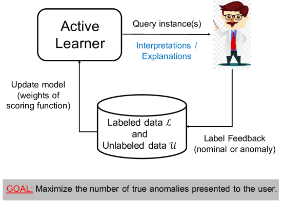
Figure 1: High-level overview of the active learning framework for anomaly detection.

We provide algorithmic solutions for key elements of this active learning framework:

• Initializing the parameters ${\bf\Theta}$ of the scoring function Score(${\bf x}$) based on a novel insight for anomaly detection ensembles.

• Query selection strategies to improve the effectiveness of active learning.

• Updating the weights of scoring function based on label feedback.

• Updating ensemble members as needed to support the streaming data setting.

• Generating interpretations and explanations for anomalous instances to improve the usability of human-in-the-loop anomaly detection systems.

4 Insights: Suitability of Ensembles for Active Learning

In this section, we show how anomaly detection ensembles are naturally suited for active learning as motivated by the active learning theory for standard classification. The key insights presented here are in the context of a linear combination of ensemble scores.

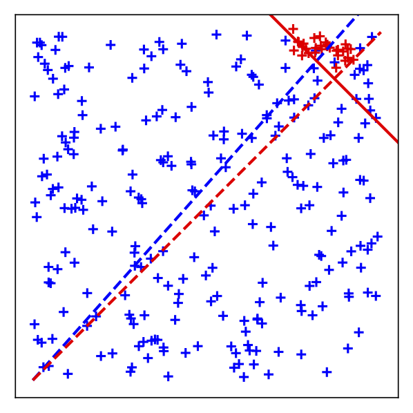
(a) C1: Common case

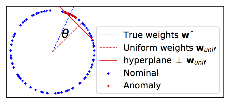
(b) C2: Similar to Active Learning theory

(c) C3: IFOR case

Figure 2: Illustration of candidate score distributions from an ensemble in 2D. The two axes represent two different ensemble members.

Without loss of generality, we assume that all scores from the members of an ensemble of anomaly detectors are normalized (i.e., they lie in $[-1,1]$ or $[0,1]$), with higher scores implying more anomalous. For the following discussion, ${\mathbf{w}}_{unif}\in\mathds{R}^{m}$ represents a vector of equal values, and $||{\mathbf{w}}_{unif}||=1$. Figure 2 illustrates a few possible distributions of normalized scores from the ensemble members in 2D. When ensemble members are “good”, they assign higher scores to anomalies and push them to an extreme region of the score space as illustrated in case C1 in Figure 2a. This makes it easier to separate anomalies from nominals by a hyperplane. Most theoretical research on active learning for classification (?, ?, ?, ?, ?) makes simplifying assumptions such as uniform data distribution over a unit sphere and with homogeneous (i.e., passing through the origin) hyperplanes. However, for anomaly detection, arguably, the idealized setup is closer to case C2 (Figure 2b), where non-homogeneous decision boundaries are more important. We present empirical evidence (Section 7), which shows that scores from the state-of-the-art Isolation Forest (IFOR) detector are distributed in a similar manner as case C3 (Figure 2c). C3 and C2 are similar in theory (for active learning) because both involve searching for the optimum non-homogeneous decision boundary. In all cases, the common theme is that when the ensemble members are ideal, then the scores of true anomalies tend to lie in the farthest possible location in the positive direction of the uniform weight vector ${\bf w}_{unif}$ by design. Consequently, the average score for an instance across all ensemble members works well for anomaly detection. However, not all ensemble members are ideal in practice, and the true weight vector (${\bf w}^{*}$) is displaced by an angle $\theta$ from ${\bf w}_{unif}$. Figure 3c shows an illustration of this scenario on a Toy dataset. In large datasets, even a small misalignment between ${\bf w}_{unif}$ and ${\bf w}^{*}$ results in many false positives. While the performance of ensemble on the basis of the AUC metric may be high, the detector could still be impractical for use by analysts.

The property, that the misalignment is usually small, can be leveraged by active learning to learn the optimal weights efficiently. To understand this, observe that the top-ranked instances are close to the decision boundary and are therefore, in the uncertainty region. The key idea is to design a hyperplane that passes through the uncertainty region which then allows us to select query instances by uncertainty sampling. Selecting instances on which the model is uncertain for labeling is efficient for active learning (?, ?). Specifically, greedily selecting instances with the highest scores is first of all more likely to reveal anomalies (i.e., true positives), and even if the selected instance is nominal (i.e., false positive), it still helps in learning the decision boundary efficiently. This is an important insight and has significant practical implications.

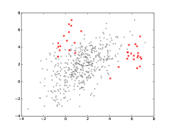
(a) Toy dataset

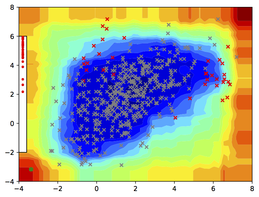
(b) Anomaly scores

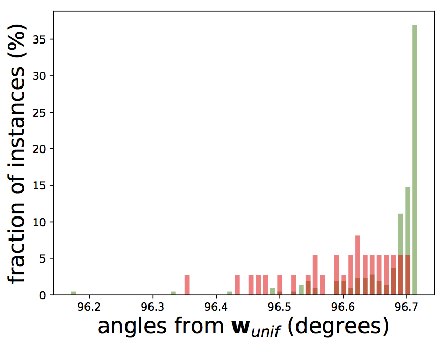
(c) Angles

Figure 3: Isolation Tree. (a) Toy dataset (?) which will be used as the running example through out the text to illustrate the ideas. Red points are anomalies and black points are nominals. (b) Anomaly scores assigned by IFOR to the Toy dataset. (c) Histogram distribution of the angles between score vectors from IFOR and ${\mathbf{w}}_{unif}$. The red and green histograms show the angle distributions for anomalies and nominals respectively. Since the red histograms are closer to the left, anomalies are aligned closer to ${\mathbf{w}}_{unif}$.

Summary. When detecting anomalies with an ensemble of detectors:

1. It is compelling to always apply active learning.

2. The greedy strategy of querying the labels for top ranked instances is efficient, and is therefore a good yardstick for evaluating the performance of other querying strategies as well.

3. Learning a decision boundary with active learning that generalizes to unseen data helps in limited-memory or streaming data settings.

The second point will be particularly significant when we evaluate a different querying strategy to enhance the diversity of discovered anomalies as part of this work. In the above discussion, we presented the insight related to the uniform prior in the context of linear score combinations only. However, we leverage the same insight in the context of a more general combination strategy as part of our GLocalized Anomaly Detection (GLAD) algorithm (Section 6).

5 Active Learning Algorithms for Tree-based Ensembles

In this section, we describe a series of algorithms for active learning with tree-based ensembles. First, we present the strengths of tree-based anomaly detector ensembles and describe one such algorithm referred as Isolation Forest in more depth (Section 5.1). Second, we present a novel formalism called compact description that describes groups of instances compactly using a tree-based model, and apply it to improve the diversity of instances selected for labeling and to generate succinct interpretable rules (Section 5.2). Third, we describe an algorithm to update the weights of the scoring function based on label feedback in the batch setting, where the entire data is available at the outset (Section 5.3). Fourth, we describe algorithms to support streaming setting, where the data comes as a continuous stream (Section 5.4).

5.1 Tree-based Anomaly Detection Ensembles

Ensemble of tree-based anomaly detectors have several attractive properties that make them an ideal candidate for active learning:

• They can be employed to construct large ensembles inexpensively.

• Treating the nodes of tree as ensemble members allows us to both focus our feedback on fine-grained subspaces as well as increase the capacity of the model in terms of separating anomalies from nominals.

• Since some of the tree-based models such as Isolation Forest (IFOR) (?), HS Trees (HST) (?), and RS Forest (RSF) (?) are state-of-the-art unsupervised detectors (?, ?), it is a significant gain if their performance can be improved with minimal label feedback.

In this work, we will focus mainly on IFOR because it performed best across all datasets (?). However, we also present results on HST and RSF wherever applicable.

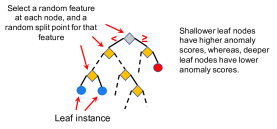
Figure 4: Illustration of Isolation tree from (?).

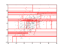
(a) One isolation tree

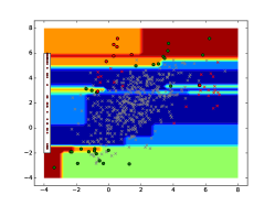
(b) Scores from one tree

Figure 5: Illustration of Isolation Tree on simple data. (a) A single isolation tree for the Toy dataset (Figure 3a). (b) Regions having deeper red belong to leaf nodes which have shorter path lengths from the root and correspondingly, higher anomaly scores. Regions having deeper blue correspond to longer path lengths and lower anomaly scores.

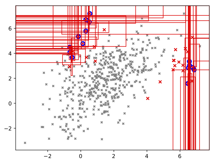
(a) IFOR

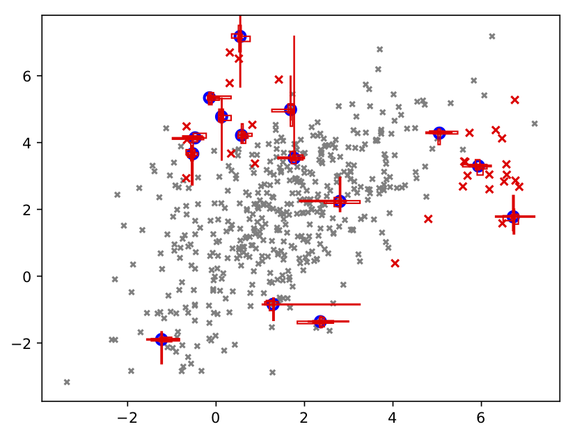
(b) HST (depth=$15$)

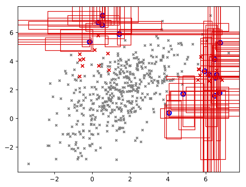
(c) HST (depth=$8$)

Figure 6: Illustration of differences among different tree-based ensembles. The red rectangles show the union of the $5$ most anomalous subspaces across each of the $15$ most anomalous instances (blue). These subspaces have the highest influence in propagating feedback across instances through gradient-based learning under our model. HST has fixed depth which needs to be high for accuracy (recommended $15$ (?)). IFOR has adaptive height and most anomalous subspaces are shallow. Higher depths are associated with smaller subspaces which are shared by fewer instances. As a result, feedback on any individual instance gets passed on to many other instances in IFOR, but to fewer instances in HST. RSF has similar behavior as HST. We set the depth for HST (and RSF (?)) to $8$ (Figure 6c) in our experiments in order to balance accuracy and feedback efficiency.

Isolation Forest (IFOR) comprises of an ensemble of isolation trees. Each tree partitions the original feature space at random by recursively splitting an unlabeled dataset. At every tree-node, first a feature is selected at random, and then a split point for that feature is sampled uniformly at random (Figure 4). This partitioning operation is carried out until every instance reaches its own leaf node. The key idea is that anomalous instances, which are generally isolated in the feature space, reach the leaf nodes faster by this partitioning strategy than nominal instances which belong to denser regions (Figure 5). Hence, the path from the root node is shorter to the leaves of anomalous instances when comapred to the leaves of nominal instances. This path length is assigned as the unnormalized score for an instance by an isolation tree. After training an IFOR with $T$ trees, we extract the leaf nodes as the members of the ensemble. Such members could number in the thousands (typically $4000-7000$ when $T=100$). Assume that a leaf is at depth $l$ from the root. If an instance belongs to the partition defined by the leaf, it gets assigned a score $-l$ by the leaf, else $0$. As a result, anomalous instances receive higher scores on average than nominal instances. Since every instance belongs to only a few leaf nodes (equal to $T$), the score vectors are sparse resulting in low memory and computational costs.

HST and RSF apply different node splitting criteria than IFOR, and compute the anomaly scores on the basis of the sample counts and densities at the nodes. We apply log-transform to the leaf-level scores so that their unsupervised performance remains similar to the original model and yet improves with feedback. The trees in HST and RSF have a fixed depth which needs to be larger in order to improve the accuracy. In contrast, trees in IFOR have adaptive depth and most anomalous subspaces are shallow. Larger depths are associated with smaller subspaces, which are shared by fewer instances. As a result, feedback on any individual instance gets passed on to very few instances in HST and RSF, but to much more number of instances in IFOR. Therefore, it is more efficient to incorporate feedback in IFOR than it is in HST or RSF (see Figure 6).

5.2 Compact Description Formalism and Applications to Diversified Querying and Interpretability

In this section, we first describe the compact description formalism to describe a group of instances. Subsequently, we propose algorithms for selecting diverse instances for querying and to generate succinct interpretable rules using compact description.

Compact Description (CD). The tree-based model assigns a weight and an anomaly score to each leaf (i.e., subspace). We denote the vector of leaf-level anomaly scores by ${\bf d}$, and the overall anomaly scores of the subspaces (corresponding to the leaf-nodes) by ${\bf a}=\left[a_{1},...,a_{m}\right]={\bf w}\circ{\bf d}$, where $\circ$ denotes element-wise product operation. The score $a_{i}$provides a good measure of the relevance of the $i$-th subspace. This relevance for each subspace is determined automatically through the label feedback. Our goal is to select a small subset of the most relevant and “compact” (by volume) subspaces which together contain all the instances in a group that we want to describe. We treat this problem as a specific instance of the set covering problem. We illustrate this idea on a synthetic dataset in Figure 7. This approach can be potentially interpreted as a form of non-parametric clustering.

Let $\mathcal{Z}$ be the set of instances that we want to describe, where $|\mathcal{Z}|=p$. For example, $\mathcal{Z}$ could correspond to the set of anomalous instances discovered by our active learning approach. Let ${\bf s}_{i}$ be the $\delta$ most relevant subspaces (i.e., leaf nodes) which contain ${\bf z}_{i}\in\mathcal{Z},i={1,...,p}$. Let $\mathcal{S}=s_{1}\cup...\cup s_{p}$ and $|\mathcal{S}|=k$. Denote the volumes of the subspaces in $\mathcal{S}$ by the vector ${\bf v}\in\mathbb{R}^{k}$. Suppose ${\bf x}\in\{0,1\}^{k}$ is a binary vector which contains $1$ in locations corresponding to the subspaces in $\mathcal{S}$ which are included in the covering set, and $0$ otherwise. Let ${\bf u}_{i}\in\{0,1\}^{k}$ denote a vector for each instance ${\bf z}_{i}\in\mathcal{Z}$ which contains $1$ in all locations corresponding to subspaces in $s_{i}$. Let ${\bf U}=[{\bf u}_{1}^{T},...,{\bf u}_{n}^{T}]^{T}$. A compact set of subspaces ${\bf S}^{*}$ which contains (i.e., describes) all the candidate instances can be computed using the optimization formulation in Equation 1. We employ an off-the-shelf ILP solver (CVX-OPT) to solve this problem.

$${\bf S}^{*} =\operatorname*{arg\,min}_{{\bf x}\in\{0,1\}^{k}}\;{\bf x}\cdot{\bf v}$$ (1)

s.t. $${\bf U}\cdot{\bf x}\geq{\bf 1}\text{ (where ${\bf 1}$ is a column vector of $p$ 1's)}$$

Applications of Compact Description. Compact descriptions have multiple uses including:

• Discovery of diverse classes of anomalies very quickly by querying instances from different subspaces of the description.

• Improved interpretability of anomalous instances. We assume that in a practical setting, the analyst(s) will be presented with instances along with their corresponding description(s). Additional information can be derived from the description and shown to the analyst (e.g., number of instances in each compact subspace), which can help prioritize the analysis.

In this work, we present empirical results on improving query diversity and also compare with another state-of-the-art algorithm that extracts interpretations (?).

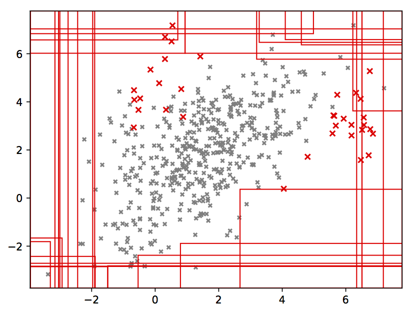
(a) Baseline

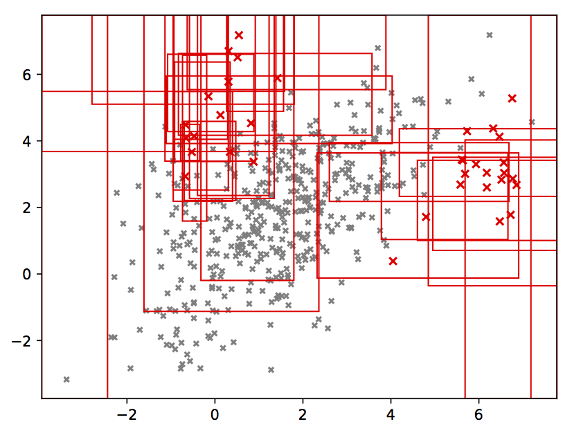
(b) Active Anomaly Detection

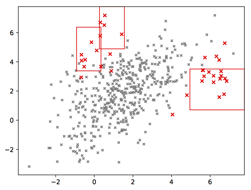
(c) Compact Description

Figure 7: Top $30$ subspaces ranked by ${\bf w}\circ{\bf d}$ (relevance). Red points are anomalies. (a) shows the top $30$ most relevant subspaces (w.r.t their anomalousness) without any feedback. We can see that initially these subspaces simply correspond to the exterior regions of the dataset. Our active anomaly detection approach learns the true relevance of subspaces via label feedback. (b) shows that after incorporating the labels of $35$ instances, the subspaces around the labeled anomalies have emerged as the most relevant. (c) shows the set of important subspaces which compactly cover all labeled anomalies. These were computed by solving Equation 1. Note that the compact subspaces only cover anomalies that were discovered in the $35$ feedback iterations. Anomalies which were not detected are likely to fall outside these compact subspaces.

Diversity-based Query Selection Strategy. In Section 4, we reasoned that the greedy strategy of selecting top-scored instances (referred as Select-Top) for labeling is efficient. However, this strategy might lack diversity in the types of instances presented to the human analyst. It is likely that different types of instances belong to different subspaces in the original feature space. Our proposed strategy (Select-Diverse), which is described next, is intended to increase the diversity by employing tree-based ensembles and compact description to select groups of instances from subspaces that have minimum overlap.

Algorithm 1 Select-Diverse (${\mathbf{X}}$, $b$, $n$)

  Input: Unlabeled dataset ${\mathbf{X}}$, # instances to select $b$, # candidate instances $n$ ($n\geq b$)

  Let $\mathcal{Z}$ = $n$ top-ranked instances as candidates $\subseteq{\mathbf{X}}$ (blue points in Figure 8a)

  Let ${\bf S}^{*}$ = subspaces with Equation 1 that contain $\mathcal{Z}$ (rectangles in Figures 8b and 8c)

  Set ${\bf Q}=\emptyset$

  while $|{\bf Q}|<b$ do

     Let ${\bf x}$ = instance with highest anomaly score $\in\mathcal{Z}$ s.t. ${\bf x}$ has minimal

                  overlapping regions in ${\bf S}^{*}$ with instances in ${\bf Q}$

     Set ${\bf Q}={\bf Q}\cup\{{\bf x}\}$ (green circles in Figure 8c)

     Set $\mathcal{Z}=\mathcal{Z}\setminus\{{\bf x}\}$

  end while

  return  ${\bf Q}$

Assume that the human analyst can label a batch of $b$ instances, where $b>1$, in each feedback iteration. Algorithm 1 employs the compact description to achieve this diversity. The algorithm first selects $n$ ($>b$) top-ranked anomalous instances $\mathcal{Z}$ and computes the corresponding compact description (small set of subspaces ${\bf S}^{*}$). Subsequently, performs an iterative selection of $b$ instances from $\mathcal{Z}$ by minimizing the overlap in the corresponding subspaces from ${\bf S}^{*}$. Figure 8 provides an illustration comparing Select-Top and Select-Diverse query selection strategies.

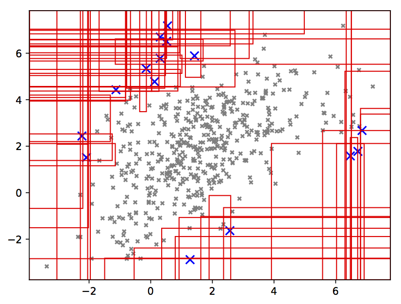
(a) Candidate Subspaces

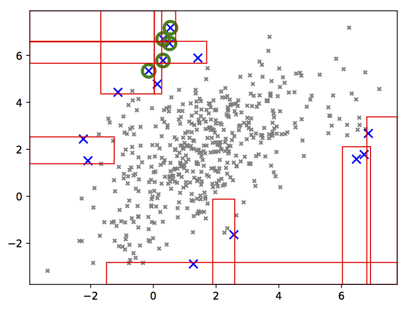
(b) Select-Top

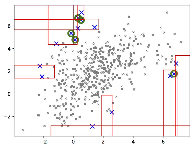
(c) Select-Diverse

Figure 8: Illustration of compact description and diversity of selected instances for labeling using IFOR. Most anomalous $15$ instances (blue checks) are selected as the query candidates. The red rectangles in (a) form the union of the $\delta$ ($=5$ works well in practice) most relevant subspaces across each of the query candidates. (b) and (c) show the most “compact” set of subspaces which together cover all the query candidates. (b) shows the most anomalous $5$ instances (green circles) selected by the greedy Select-Top strategy. (c) shows the $5$ “diverse” instances (green circles) selected by Select-Diverse.

Interpretable Explanations from Subspaces. While Equation 1 helps in generating descriptions to improve query diversity, it lacks consideration for easy interpretability by a human analyst. Motivated by the research in interpretability for classification problems (?), we state the following desiderata for interpretability of anomalies:

• Descriptions (of anomalies) should be simple. Subspaces in the case of tree-based models are defined by ranges of feature values which can be translated to predicate rules. A feature range which does not have either a minimum or a maximum value (i.e., $\pm\infty$) requires fewer predicates for defining the corresponding rule and simplifies the subspace definition.

• Descriptions should be precise, i.e., they should include few nominals (false-positives). The absence of this property would result in descriptions with high recall but low precision.

Keeping the above considerations in mind, we modify Equation 1 as follows:

$${\bf S}^{*} =\operatorname*{arg\,min}_{{\bf x}\in\{0,1\}^{k}}\;{\bf x}\cdot({\bf v}\circ({\bf 1}_{k}+{\bf\eta})+{\bf\varsigma})$$ (2)

s.t. $${\bf U}\cdot{\bf x}\geq{\bf 1}_{p}$$

where $${\bf x},{\bf v},p,k\text{ are the same as defined for Equation~{}\ref{eqn:compact}}$$

$${\bf 1}_{k}\text{ is a column vector of $k$ 1's}$$

$${\bf 1}_{p}\text{ is a column vector of $p$ 1's}$$

$${\bf\eta}=\{\eta_{1},\cdots,\eta_{k}\}\text{ are the number of `nominals' in the subspaces in }\mathcal{S}$$

$${\bf\varsigma}=\{\varsigma_{1},\cdots,\varsigma_{k}\}\text{ are the complexities (function of rule lenghts) of subspaces in }\mathcal{S}$$

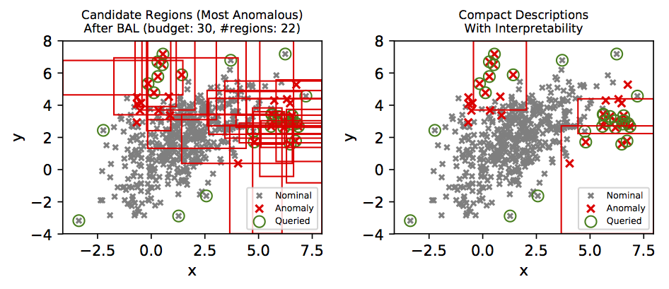
(a)

Figure 9: Illustration of interpretable rules on Toy dataset. The left figure shows all candidate regions after $30$ feedback iterations. The figure on the left shows the interpretable description for anomalies computed by Algorithm 2. The interpretable descriptions are translated to the following rule: predict ‘anomaly’ if ((x > 4.436513) & (y > 2.238837) & (y <= 4.395921)) or ((x > 3.658627) & (y <= 2.716822)) or ((x > -0.431709) & (x <= 2.033541) & (y > 3.703597))

Algorithm 2 employs Equation 2 to generate interpretable descriptions for all anomalies in a group of labeled instances $\mathcal{L}$. The algorithm also takes as input a set of unlabeled instances $\mathcal{U}$ from which it samples a set of pseudo “nominals” denoted by $\mathcal{L}_{u}$. The labeled nominals in $\mathcal{L}$ together with $\mathcal{L}_{u}$ are then used to improve the precision of the output descriptions. The number of nominals in $\mathcal{L}\cup\mathcal{L}_{u}$ which fall within a subspace $s$ is computed as $\eta_{s}=\texttt{num\_nominals}(s,\mathcal{L}\cup\mathcal{L}_{u})$. Since a precise description of anomalies should exclude nominals as much as possible, Equation 2 penalizes a subspace $s$ in proportion to $\eta_{s}$. Furthermore, Algorithm 2 retains only those subspaces whose precision is greater than a threshold, i.e., $\texttt{precision}(s,\mathcal{L}\cup\mathcal{L}_{u})\geq t$. Subspaces which are selected for the descriptions can be represented as rules based on their feature-ranges. A rule has the same length as the number of feature-range predicates required to define a description. Longer rules are harder for an analyst to understand. Therefore, we define the complexity $\varsigma_{s}$ of a subspace $s$ as a function of its rule length: $\varsigma_{s}=2^{\texttt{rule\_length}(s)-1}$. Equation 2 penalizes a subspace by its complexity and therefore, encourages selection of subspaces which are simpler to define. Figure 9 illustrates the rules generated on the Toy dataset.

At a broader level, we start with as many candidate subspaces for descriptions as the number of leaves in the forest. Typically, these are few thousands in number. The label feedback from human analyst helps in automatically identifying the most relevant candidates for Algorithm 2, which then applies additional filters using Equation 2 and the precision of subspaces. Thus, Algorithm 2 tries to efficiently select an optimal subset from thousands of subspaces via stepwise selection and filtering.

Algorithm 2 Interpretable-Descriptions ($\mathcal{L}$, $\mathcal{U}$, $u$, $t$)

  Input: Labeled set we want to describe $\mathcal{L}$ (having anomalies as well as nominals),

      unlabeled set from which we sample “nominals” $\mathcal{U}$,

      number of additional instances to sample as “nominals” $u$,

      precision threshold $t\in[0,1]$

  Let $\mathcal{L}_{u}$ = select $u$ random instances from $\mathcal{U}$ and label them as ‘nominal’

  Let $\mathcal{Z}=\{{\bf x}\in\mathcal{L}\cup\mathcal{L}_{u}:{\bf x}\text{ is labeled `anomaly'}\}$

  Let $\mathcal{S}$ = candidate subspaces for describing instances in $\mathcal{Z}$

  Let ${\bf v}=\{\texttt{volume}(s):s\in\mathcal{S}\}$

  Let ${\bf\eta}=\{\texttt{num\_nominals}(s,\mathcal{L}\cup\mathcal{L}_{u}):s\in\mathcal{S}\}$

  Let ${\bf\varsigma}=\{2^{\texttt{rule\_length}(s)-1}:s\in\mathcal{S}\}$

  Let ${\bf S}^{*}$ = compute subspaces with Equation 2

  return  ${\bf Q}=\{s:s\in{\bf S}^{*}\text{ and }\texttt{precision}(s,\mathcal{L}\cup\mathcal{L}_{u})\geq t\}$

5.3 Algorithmic Approach to Update Weights of Scoring Function

In this section, we provide an algorithm to update weights of the scoring function in the batch active learning (BAL) setting: the entire data ${\bf D}$ is available at the outset.

Recall that our scoring function is of the following form: Score(${\bf x}$) = ${\mathbf{w}}\cdot{\bf z}$, where ${\bf z}\in\mathds{R}^{m}$ corresponds to the scores from anomaly detectors for instance ${\bf x}$. We extend the AAD approach (based on LODA projections) (?) to update the weights for tree-based models. AAD makes the following assumptions: (1) $\tau$ fraction of instances (i.e., $n\tau$) are anomalous, and (2) Anomalies should lie above the optimal hyperplane while nominals should lie below. AAD tries to satisfy these assumptions by enforcing constraints on the labeled examples while learning the weights of the hyperplane. If the anomalies are rare and we set $\tau$ to a small value, then the two assumptions make it more likely that the hyperplane will pass through the region of uncertainty. Our previous discussion then suggests that the optimal hyperplane can now be learned efficiently by greedily asking the analyst to label the most anomalous instance in each feedback iteration. We simplify the AAD formulation with a more scalable unconstrained optimization objective, and refer to this version as BAL. Crucially, the ensemble weights are updated with an intent to maintain the hyperplane in the region of uncertainty through the entire budget $B$. The batch active learning approach is presented in Algorithm 3. BAL depends on only one hyper-parameter $\tau$.

We first define the hinge loss $\ell(q,{\mathbf{w}};({\mathbf{z}}_{i},y_{i}))$ in Equation 7 that penalizes the model when anomalies are assigned scores lower than $q$ and nominals higher. Equation 8 then formulates the optimization problem for learning the optimal weights in Line 14 of the batch algorithm (Algorithm 3). Figure 10 illustrates how BAL changes the anomaly score contours across feedback iterations on the synthetic dataset using an isolation forest with $100$ trees.

$$\ell(q,{\mathbf{w}};({\mathbf{z}}_{i},y_{i}))=$$

$$\left\{\begin{array}[]{lr}0&{\mathbf{w}}\cdot{\mathbf{z}}_{i}\geq q\text{ and $y_{i}=+1$}\\ 0&{\mathbf{w}}\cdot{\mathbf{z}}_{i}<q\text{ and $y_{i}=-1$}\\ (q-{\mathbf{w}}\cdot{\mathbf{z}}_{i})&{\mathbf{w}}\cdot{\mathbf{z}}_{i}<q\text{ and $y_{i}=+1$}\\ ({\mathbf{w}}\cdot{\mathbf{z}}_{i}-q)&{\mathbf{w}}\cdot{\mathbf{z}}_{i}\geq q\text{ and $y_{i}=-1$}\end{array}\right.$$ (7)

$${\mathbf{w}}^{(t)} =\operatorname*{arg\,min}_{{\mathbf{w}}}\sum_{s\in\{-,+\}}\left(\frac{1}{|{\mathbf{H}}_{s}|}\sum_{{\mathbf{z}}_{i}\in{\mathbf{H}}_{s}}\ell(\hat{q}_{\tau}({{\mathbf{w}}^{(t-1)}}),{\mathbf{w}};({\mathbf{z}}_{i},y_{i}))\right.$$

$$\left.\qquad\qquad+\frac{1}{|{\mathbf{H}}_{s}|}\sum_{{\mathbf{z}}_{i}\in{\mathbf{H}}_{s}}\ell({\mathbf{z}}_{\tau}^{(t-1)}\cdot{\mathbf{w}},{\mathbf{w}};({\mathbf{z}}_{i},y_{i}))\right)$$

$$\qquad\qquad+\lambda^{(t)}\|{\mathbf{w}}-{\mathbf{w}}_{unif}\|^{2}$$ (8)

$$\text{where, }\mathbf{w}_{unif}=[\frac{1}{\sqrt{m}},\ldots,\frac{1}{\sqrt{m}}]^{T},\text{ and,}$$

$${\mathbf{z}}_{\tau}^{(t-1)}\text{ and }\hat{q}_{\tau}({{\mathbf{w}}^{(t-1)}})\text{ are computed by ranking}$$

anomaly scores with $${\mathbf{w}}={\mathbf{w}}^{(t-1)}$$

$\lambda^{(t)}$ determines the influence of the prior. For the batch setup, we set $\lambda^{(t)}=\frac{0.5}{|{\bf H}_{+}|+|{\bf H}_{-}|}$ such that the prior becomes less important as more instances are labeled. When there are no labeled instances, $\lambda^{(t)}$ is set to $\frac{1}{2}$. The third and fourth terms of Equation 8 encourage the scores of anomalies in $\mathbf{H}_{+}$ to be higher than that of ${\mathbf{z}}_{\tau}^{(t-1)}$ (the $n\tau$-th ranked instance from the previous iteration), and the scores of nominals in $\mathbf{H}_{-}$ to be lower than that of ${\mathbf{z}}_{\tau}^{(t-1)}$. We employ gradient descent to learn the optimal weights ${\mathbf{w}}$ in Equation 8. Our prior knowledge that ${\bf w}_{unif}$ is a good prior provides a good initialization for gradient descent. We later show empirically that ${\bf w}_{unif}$ is a better starting point than random weights.

Algorithm 3 Batch-AL ($B$, ${\mathbf{w}}^{(0)}$, ${\mathbf{H}}$, ${\mathbf{H}}_{+}$, ${\mathbf{H}}_{-}$)

  Input: Query budget $B$, initial weights ${\mathbf{w}}^{(0)}$, unlabeled instances ${\mathbf{H}}$,

      labeled instances ${\mathbf{H}}_{+}$ and ${\mathbf{H}}_{-}$

  Set $t=0$

  while $t\leq B$ do

     Set $t=t+1$

     Set ${\mathbf{a}}={\mathbf{H}}\cdot{\mathbf{w}}$ (i.e., ${\mathbf{a}}$ is the vector of anomaly scores)

     Let ${\bf q}={\mathbf{z}}_{i}$, where $i=\operatorname*{arg\,max}_{i}(a_{i})$

     Get $y_{i}\in\{-1,+1\}$ for ${\mathbf{q}}$ from analyst

     if $y_{i}=+1$ then

        Set ${\mathbf{H}}_{+}=\{{\bf z}_{i}\}\cup{\mathbf{H}}_{+}$

     else

        Set ${\mathbf{H}}_{-}=\{{\bf z}_{i}\}\cup{\mathbf{H}}_{-}$

     end if

14:     Set ${\mathbf{H}}={\mathbf{H}}\setminus{\mathbf{z}}_{i}$

     ${\mathbf{w}}^{(t)}$ = learn new weights; normalize $\|{\mathbf{w}}^{(t)}\|=1$

  end while

  return  ${\mathbf{w}}^{(t)}$, ${\mathbf{H}}$, ${\mathbf{H}}_{+}$, ${\mathbf{H}}_{-}$

(a) Initial scores

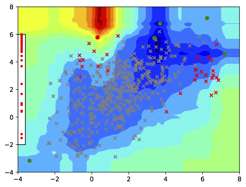
(b) 8 iterations

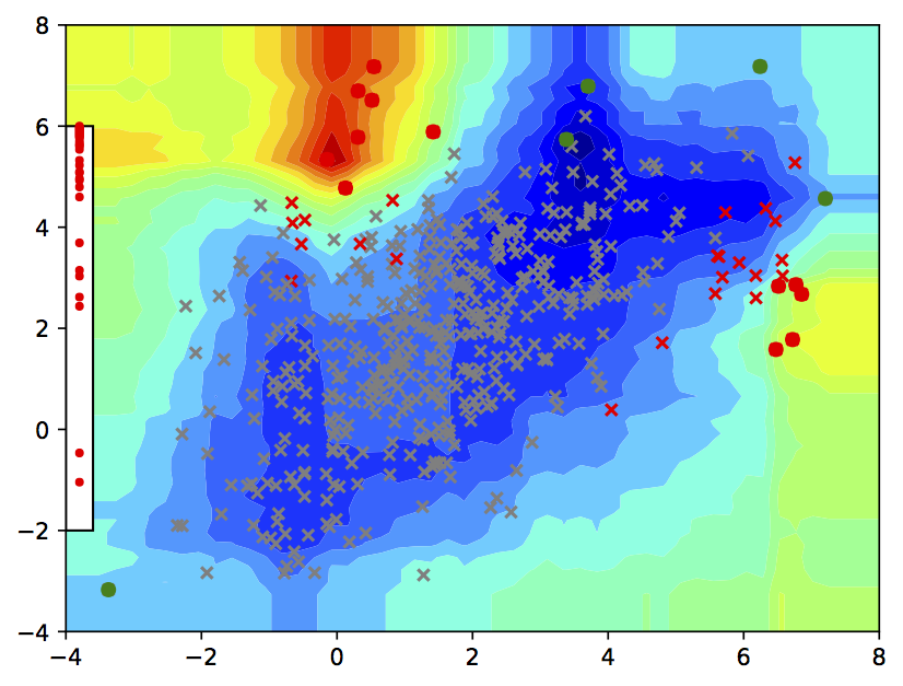
(c) 16 iterations

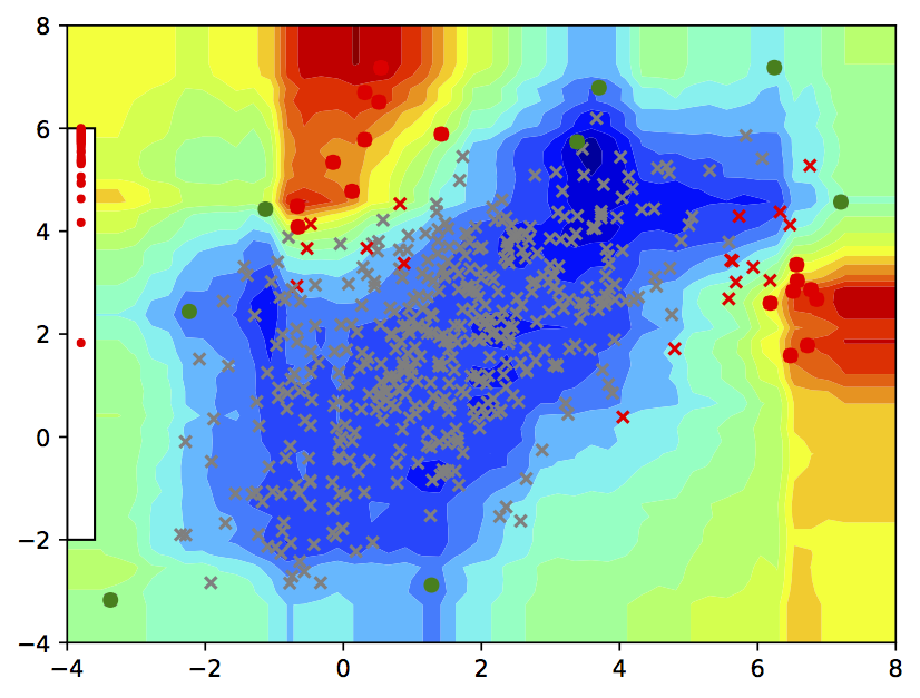
(d) 24 iterations

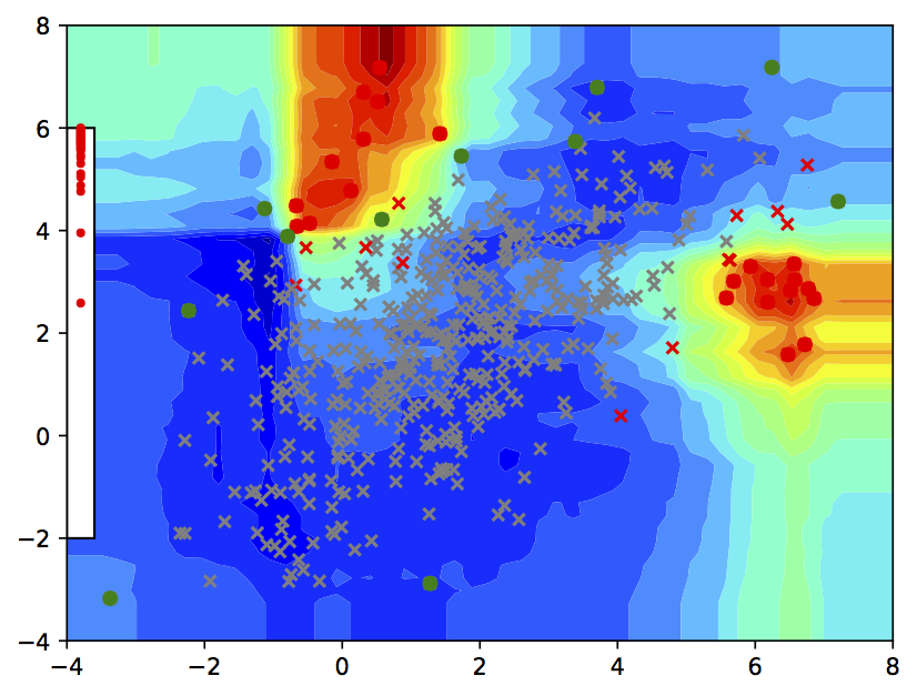
(e) 32 iterations

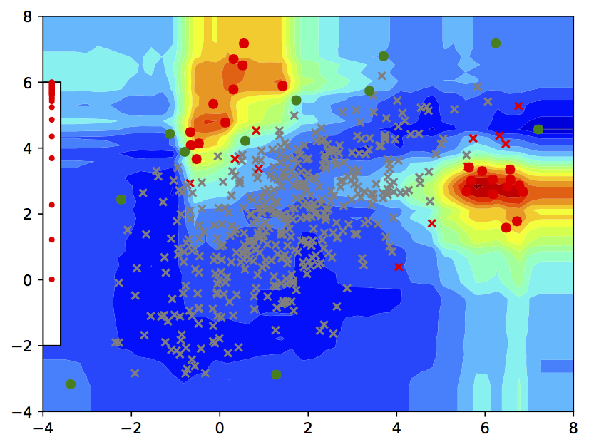
(f) 34 iterations

Figure 10: Score contours across $34$ BAL feedback iterations on the Toy dataset (Figure 3a).

5.4 Algorithms for Active Anomaly Detection in Streaming Data Setting

In this section, we describe algorithms to support active anomaly detection using tree-based ensembles in the streaming data setting.

In the streaming setting, we assume that the data is input to the algorithm continuously in windows of size $K$ and is potentially unlimited. The framework for the streaming active learning (SAL) is shown in Algorithm 4. Initially, we train all the members of the ensemble with the first window of data. When a new window of data arrives, the underlying tree model is updated as follows: in case the model is an HST or RSF, only the node counts are updated while keeping the tree structures and weights unchanged; whereas, if the model is an IFOR, a subset of the current set of trees is replaced as shown in Update-Model (Algorithm 4). The updated model is then employed to determine which unlabeled instances to retain in memory, and which to “forget”. This step, referred to as Merge-and-Retain, applies the simple strategy of retaining only the most anomalous instances among those in the memory and in the current window, and discarding the rest. Next, the weights are fine-tuned with analyst feedback through an active learning loop similar to the batch setting with a small budget $Q$. Finally, the next window of data is read, and the process is repeated until the stream is empty or the total budget $B$ is exhausted. In the rest of this section, we will assume that the underlying tree model is IFOR.

When we replace a tree in Update-Model, its leaf nodes and corresponding weights get discarded. On the other hand, adding a new tree implies adding all its leaf nodes with weights initialized to a default value $v$. We first set $v=\frac{1}{\sqrt{m^{\prime}}}$ where $m^{\prime}$ is the total number of leaves in the new model, and then re-normalize the updated ${\bf w}$ to unit length.

The stream active learning framework is presented in Algorithm 4. In all the SAL experiments, we set the number of queries per window $Q=20$, and $\lambda^{(t)}=\frac{1}{2}$.

Algorithm 4 Stream-AL ($K$, $B$, $Q$, $\mathcal{E}^{(0)}$, ${\mathbf{X}}_{0}$, ${\mathbf{w}}^{(0)}$, $\alpha_{KL}$)

  Input: Stream window size $K$, total query budget $B$,

      queries per window $Q$, anomaly detector ensemble $\mathcal{E}^{(0)}$,

      initial instances ${\mathbf{X}}_{0}$ (used to create $\mathcal{E}^{(0)}$), initial weights ${\mathbf{w}}^{(0)}$,

      significance level $\alpha_{KL}$

  

  Set ${\mathbf{H}}={\mathbf{H}}_{+}={\mathbf{H}}_{-}=\emptyset$

  // initialize KL-divergence baselines

  Set $q_{KL}^{(0)}$ = Get-KL-Threshold(${\mathbf{X}}_{0}$, $\mathcal{E}^{(0)}$, $\alpha_{KL}$, $10$)

  Set $\mathcal{P}^{(0)}$ = Get-Ensemble-Distribution(${\mathbf{X}}_{0}$, $\mathcal{E}^{(0)}$)

  

  Set $t=0$

  while $<$stream is not empty$>$ do

     Set $t=t+1$

     Set ${\mathbf{X}}_{t}$ = $K$ data instances from stream

     Set ${\mathbf{H}}_{t}$ = transform ${\mathbf{X}}_{t}$ to ensemble features

     

     // Update-Model either updates node counts (e.g., for HST and RSF),

     // or replaces a fraction of the oldest trees in $\mathcal{E}$ with new

     // ones constructed using ${\mathbf{X}}_{t}$ (e.g., for IFOR)

     Set $\mathcal{E}^{(t)}$, $q_{KL}^{(t)}$, $\mathcal{P}^{(t)}$ = Update-Model(${\mathbf{X}}_{t}$, $\mathcal{E}^{(t-1)}$, $q_{KL}^{(t-1)}$, $\mathcal{P}^{(t-1)}$, $\alpha_{KL}$)

     

     // Merge-and-Retain(${\mathbf{w}}$, ${\mathbf{H}}$, $K$) retains $K$ most anomalous instances in ${\mathbf{H}}$

     Set ${\mathbf{H}}=$ Merge-and-Retain(${\mathbf{w}}^{(t-1)}$, $\{{\mathbf{H}}\cup{\mathbf{H}}_{t}\}$, $K$)

     Set ${\mathbf{w}}^{(t)}$, ${\mathbf{H}}$, ${\mathbf{H}}_{+}$, ${\mathbf{H}}_{-}$ = Batch-AL($Q$, ${\mathbf{w}}^{(t-1)}$, ${\mathbf{H}}$, ${\mathbf{H}}_{+}$, ${\mathbf{H}}_{-}$)

  end while

SAL approach can be employed in two different situations: (1) limited memory with no concept drift, and (2) streaming data with concept drift. The type of situation determines how fast the model needs to be updated in Update-Model. If there is no concept drift, we need not update the model at all. If there is a large change in the distribution of data from one window to the next, then a large fraction of members need to be replaced. When we replace a member tree in our tree-based model, all its corresponding nodes along with their learned weights have to be discarded. Thus, some of the “knowledge” is lost with the model update. In general, it is hard to determine the true rate of drift in the data. One approach is to replace, in the Update-Model step, a reasonable number (e.g. 20%) of older ensemble members with new members trained on new data. Although this ad hoc approach often works well in practice, a more principled approach is preferable.

Drift Detection Algorithm. Algorithm 5 presents a principled methodology that employs KL-divergence (denoted by $D_{KL}$) to determine which trees should be replaced. The set of all leaf nodes in a tree are treated as a set of histogram bins which are then used to estimate the data distribution. We denote the total number of trees in the model by $T$, and the $t$-th tree by $\mathcal{T}_{t}$. When $\mathcal{T}_{t}$ is initially created with the first window of data, the data from the same window is also used to initialize the baseline distribution for $\mathcal{T}_{t}$, denoted by ${\bf p}_{t}$ (Get-Ensemble-Distribution in Algorithm 7). After computing the baseline distributions for each tree, we estimate the $D_{KL}$ threshold $q_{KL}$ at the $\alpha_{KL}$ (typically $0.05$) significance level by sub-sampling (Get-KL-Threshold in Algorithm 6). When a new window is read, we first use it to compute the new distribution ${\bf q}_{t}$ (for $\mathcal{T}_{t}$). Next, if ${\bf q}_{t}$ differs significantly from ${\bf p}_{t}$ (i.e., $D_{KL}({\bf p}_{t}||{\bf q}_{t})>q_{KL}$) for at least $2\alpha_{KL}T$ trees, then we replace all such trees with new ones created using the data from the new window. Finally, if any tree in the forest is replaced, then the baseline densities for all trees are recomputed with the data in the new window.

Algorithm 5 Update-Model (${\mathbf{X}}$, $\mathcal{E}$, $q_{KL}$, $\mathcal{P}$, $\alpha_{KL}$)

  Input: Instances ${\mathbf{X}}$, anomaly detector ensemble $\mathcal{E}$,

      current KL threshold $q_{KL}$, baseline distributions $\mathcal{P}$,

      significance level $\alpha_{KL}$

  Set $T$ = number of trees in $\mathcal{E}$

  Set $\mathcal{Q}$ = Get-Ensemble-Distribution(${\mathbf{X}},\mathcal{E}$)

  Initialize $\mathbf{KL}={\mathbf{0}}\in\mathbb{R}^{T}$

  for $t\in 1..T$ do

     Set $KL_{t}=D_{KL}(\mathcal{P}_{t}||\mathcal{Q}_{t})$

  end for

  Set $S=\{t:KL_{t}>q_{KL}\}$

  if $|S|<2\alpha_{KL}T$ then

     // the number of trees with divergence is not significant

     return  $\mathcal{E},q_{KL},\mathcal{P}$

  end if

  Set $\mathcal{E}^{\prime}$ = replace trees in $\mathcal{E}$ whose indexes are in $S$, with new trees trained using $\mathbf{X}$

  // Recompute threshold and baseline distributions

  Set $q_{KL}^{\prime}$ = Get-KL-Threshold(${\mathbf{X}},\mathcal{E}^{\prime}$, $\alpha_{KL}$, $10$)

  Set $\mathcal{P}^{\prime}$ = Get-Ensemble-Distribution(${\mathbf{X}},\mathcal{E}^{\prime}$)

  return  $\mathcal{E}^{\prime},q_{KL}^{\prime},\mathcal{P}^{\prime}$

Algorithm 6 Get-KL-Threshold (${\mathbf{X}}$, $\mathcal{E}$, $\alpha_{KL}$, $n$)

  Input: Instances ${\mathbf{X}}$, anomaly detector ensemble $\mathcal{E}$,

      significance level $\alpha_{KL}$,

      repetitions of KL-divergence computations $n$

  Set $T$ = number of trees in $\mathcal{E}$

  Initialize ${\mathbf{KL}}={\mathbf{0}}\in\mathbb{R}^{T}$ // mean KL-divergence for each tree

  for $i$ in $1\cdots n$ do

     Partition ${\mathbf{X}}$ = $\{{\mathbf{A}},{\mathbf{B}}\}$ at random s.t. ${\mathbf{X}}={\mathbf{A}}\cup{\mathbf{B}}$ and $|{\mathbf{A}}|\approx|{\mathbf{B}}|$

     for $t\in 1\cdots T$ do

        Let $\mathcal{T}_{t}=t\text{-th tree in }\mathcal{E}$

        Set ${\mathbf{p}}_{A}$ = Get-Tree-Distribution(${\mathbf{A}},\mathcal{T}_{t}$)

        Set ${\mathbf{p}}_{B}$ = Get-Tree-Distribution(${\mathbf{B}},\mathcal{T}_{t}$)

        Set $KL_{t}=KL_{t}+D_{KL}({\mathbf{p}}_{A}||{\mathbf{p}}_{B})$

     end for

  end for

  Set ${\mathbf{KL}}=\frac{{\mathbf{KL}}}{n}$       // average the values

  Set $q_{KL}=(1-\alpha_{KL})\times 100\text{ quantile value in }{\mathbf{KL}}$

  return  $q_{KL}$

Algorithm 7 Get-Ensemble-Distribution (${\mathbf{X}}$, $\mathcal{E}$)

  Input: Instances ${\mathbf{X}}$, ensemble $\mathcal{E}$

  Set $T$ = number of trees in $\mathcal{E}$

  Set ${\mathcal{P}}=\emptyset$

  for $t\in 1\cdots T$ do

     Let $\mathcal{T}_{t}=t\text{-th tree in }\mathcal{E}$

     Set ${\mathbf{p}}_{t}$ = Get-Tree-Distribution(${\mathbf{X}},\mathcal{T}_{t}$)

     Set $\mathcal{P}=\mathcal{P}\cup{\mathbf{p}}_{t}$

  end for

  return  $\mathcal{P}$

Algorithm 8 Get-Tree-Distribution (${\mathbf{X}}$, $\mathcal{T}$)

  Input: Instances ${\mathbf{X}}$, tree $\mathcal{T}$

  Set ${\mathbf{p}}=$ distribution of instances in ${\mathbf{X}}$ at the leaves of $\mathcal{T}$

  return  ${\mathbf{p}}$

6 Active Learning Algorithms for Generic Ensembles

In this section, we first describe an active anomaly detection algorithm referred as GLAD that is applicable to generic (homogeneous or heterogeneous) ensemble of detectors. Subsequently, we describe a GLAD-specific approach to generate succinct explanations to help the human analyst.

6.1 GLocalized Anomaly Detection via Active Feature Space Suppression

Definition 1 (Glocal)

Reflecting or characterized by both local and global considerations.

A majority of the active learning techniques for discovering anomalies, including those presented above, employ a weighted linear combination of the anomaly scores from the ensemble members. This approach works well when the ensemble contains a large number of members which are themselves highly localized, such as the leaf nodes of tree-based detectors. However, when there are a small number of detectors in the ensemble and/or the members of the ensemble are global (such as LODA projections (?)), it is highly likely that individual detectors are incorrect in at least some local parts of the input feature space. To overcome this drawback, we propose a principled technique — GLocalized Anomaly Detection (GLAD) — which allows a human analyst to continue using anomaly detection ensembles with global behavior by learning their local relevance in different parts of the feature space via label feedback. Our GLAD algorithm automatically learns the local relevance of each ensemble member in the feature space via a neural network using the label feedback from a human analyst.

Our GLAD technique is similar in spirit to dynamic ensemble weighting (?). However, since we are in an active learning setting for anomaly detection, we need to consider two important aspects: (a) Number of labeled examples is very small (possibly none), and (b) To reduce the effort of the human analyst, the algorithm needs to be primed so that the likelihood of discovering anomalies is very high from the first feedback iteration itself.

Overview of GLAD Algorithm. We assume the availability of an ensemble $\mathcal{E}$ of $M$ (global) anomaly detectors (e.g., LODA projections) which assign scores $s_{1}({\bf x}),s_{2}({\bf x}),\cdots,s_{M}({\bf x})$ to each instance ${\bf x}\in\mathcal{X}$. Suppose that $p_{m}({\bf x})\in[0,1]$ denotes the relevance of the $m^{th}$ ensemble member for a data instance ${\bf x}$. We employ a neural network to predict the local relevance of each ensemble member. The scores of $M$ anomaly detectors are combined as follows: Score(${\bf x}$) = $\sum_{m=1}^{M}{s_{m}({\bf x})\cdot p_{m}({\bf x})}$. We incorporate the insights discussed in Section 4 for GLAD as follows. We start with the assumption that each ensemble member is uniformly relevant in every part of the input feature space. This assumption is implemented by priming a neural network referred to as FSSN (feature space suppression network) with parameters ${\bf\Theta}$ to predict the same probability value $b\in(0,1)$ for every instance in ${\bf D}$. In effect, this mechanism places a uniform prior over the input feature space $\mathcal{X}$ for the relevance of each detector. Subsequently, the algorithm receives label feedback from a human analyst and determines whether the ensemble made an error (i.e., anomalous instances are ranked at the top and scores of anomalies are higher than scores of nominals). If there was an error, the weights of FSSN are updated to suppress all erroneous detectors for similar inputs in the future. Figure 11 illustrates the different components of the GLAD algorithm (Algorithm 9) including the ensemble of anomaly detectors and the FSSN.

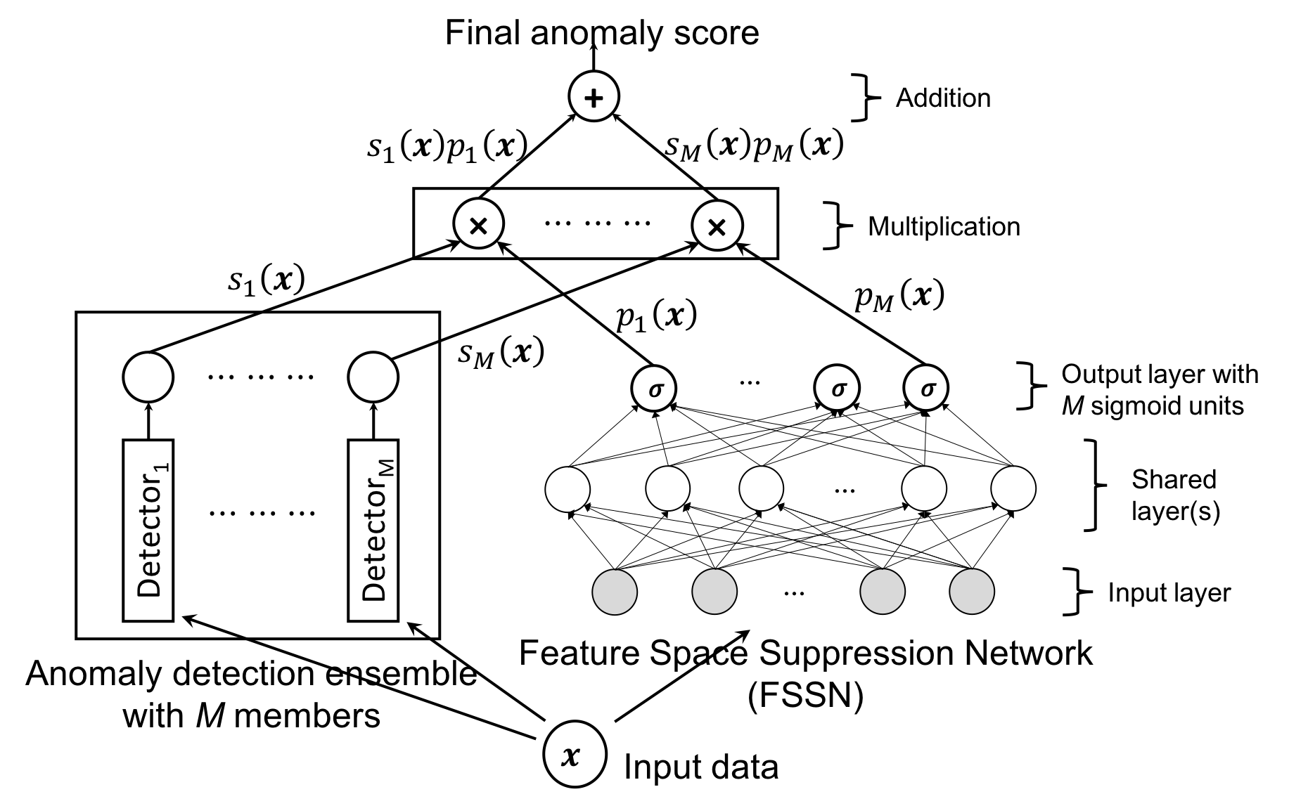
(a)

Figure 11: Overview of GLAD Algorithm. In each iteration, we select one unlabeled instance for querying, and update the weights of FSSN to adjust the local relevance of each ensemble member over all labeled instances.

Loss Function.

We employ a hinge loss similar to that in Equation 7, but tailored to the GLAD-specific score. We will denote this loss by $\ell_{AAD}({\bf x})$ (Equation 11).

$$\ell_{prior}({\bf x}) =\sum_{m=1}^{M}{-b\log(p_{m}({\bf x}))-(1-b)\log(1-p_{m}({\bf x}))}$$ (9)

$$\ell_{A}(q;({\bf x},y)) =\max(0,y(q-\text{{Score}$({\bf x})$}))$$ (10)

$$\ell_{AAD}({\bf x},y) =\ell_{A}(q_{\tau}^{(t-1)};({\bf x},y))+\ell_{A}(\text{{Score}}({\bf x}_{\tau}^{(t-1)});({\bf x},y))$$ (11)

$$\ell_{FSSN} =\frac{1}{|{\bf H}_{f}^{(t)}|}\sum_{({\bf x},y)\in{\bf H}_{f}^{(t)}}\ell_{AAD}({\bf x},y)+\frac{\lambda}{|{\bf D}|}\sum_{{\bf x}\in{\bf D}}\ell_{prior}({\bf x})$$ (12)

Feature Space Suppression Network (FSSN).

The FSSN is a neural network with $M$ sigmoid activation nodes in its output layer, where each output node is paired with an ensemble member. It takes as input an instance from the original feature space and outputs the relevance of each detector for that instance. We denote the relevance of the $m^{th}$ detector to instance ${\bf x}$ by $p_{m}({\bf x})$. The FSSN is primed using the cross-entropy loss in Equation 9 such that it outputs the same probability $b\in(0,1)$ at all the output nodes for each data instance in ${\bf D}$. This loss acts as a prior on the relevance of detectors in ensemble. When all detectors have the same relevance, the final anomaly score simply corresponds to the average score across all detectors (up to a multiplicative constant), and is a good starting point for active learning. The FSSN must have sufficient capacity to be able to learn to output the same value for every instance non-trivially. This is not hard with neural networks as the capacity can be increased simply by adding a few more hidden nodes. For improved robustness and generalization, it is preferable to select the simplest network that can achieve this goal.

After FSSN is primed, it automatically learns the relevance of the detectors based on label feedback from human analyst using the combined loss $\ell_{FSSN}$ in Equation 12, where $\lambda$ is the trade-off parameter. We set the value of $\lambda$ to 1 in all our experiments. $\mathbf{H}_{f}^{(t)}\subseteq{\bf D}$ in Equation 12 denotes the total set of instances labeled by the analyst after $t$ feedback iterations. ${\mathbf{x}}_{\tau}^{(t-1)}$ and $q_{\tau}^{(t-1)}$ denote the instance ranked at the $\tau$-th quantile and its score after the $(t-1)$-th feedback iteration. $\ell_{A}$ encourages the scores of anomalies in $\mathbf{H}_{f}$ to be higher than that of $q$, and the scores of nominals in $\mathbf{H}_{f}$ to be lower.

Algorithm 9 GLAD ($B$, $\mathcal{E}$, FSSN, ${\mathbf{D}}$, ${\mathbf{H}}_{f}$, $b$)

  Input: Query budget $B$, Ensemble $\mathcal{E}$,

      Feature Space Suppression Network FSSN with parameters ${\bf\Theta}$,

      complete dataset ${\mathbf{D}}$, labeled instances ${\mathbf{H}}_{f}\subseteq{\bf D}$, bias probability $b$

  Initialize FSSN to predict $b$ for all ${\bf x}\in{\bf D}$ // priming step

  for $t\in\{1\cdots B\}$ do

     

     // get the vector of anomaly scores for unlabeled instances

     Set ${\mathbf{a}}$ = Score(${\mathbf{D}}\setminus\{x:(x,.)\in{\bf H}_{f}\}$, $\mathcal{E}$, FSSN)

     

     // greedy query strategy: label most anomalous instance

     Let ${\bf q}={\mathbf{x}}_{i}$, where $i=\operatorname*{arg\,max}_{i}(a_{i})$

     Get label $y_{i}\in\{-1,+1\}$ for ${\mathbf{q}}$ from human analyst

     Set ${\mathbf{H}}_{f}=\{({\bf x}_{i},y_{i})\}\cup{\mathbf{H}}_{f}$

     

     Update the parameters of FSSN by minimizing loss in Equation 12

     

  end for

  return  FSSN, ${\mathbf{H}}_{f}$

Illustration of GLAD on Toy Data.

We employed a shallow neural network with $50$ hidden nodes as the FSSN. The anomaly detection ensemble comprises of the four LODA projections shown in Figure 12. Figure 12b illustrates the aspect that detectors are varying in quality. Figure 12d shows that GLAD learns useful relevance information that can be of help to the analyst.

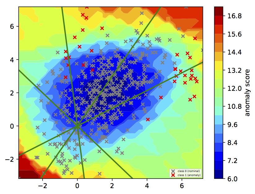
(a) Baseline LODA score contours

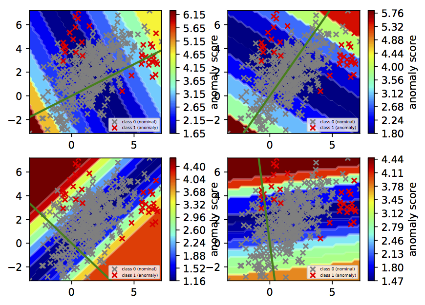
(b) Score contours for each LODA projection

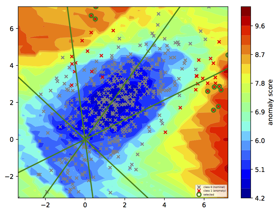
(c) Learned scores after 30 iterations

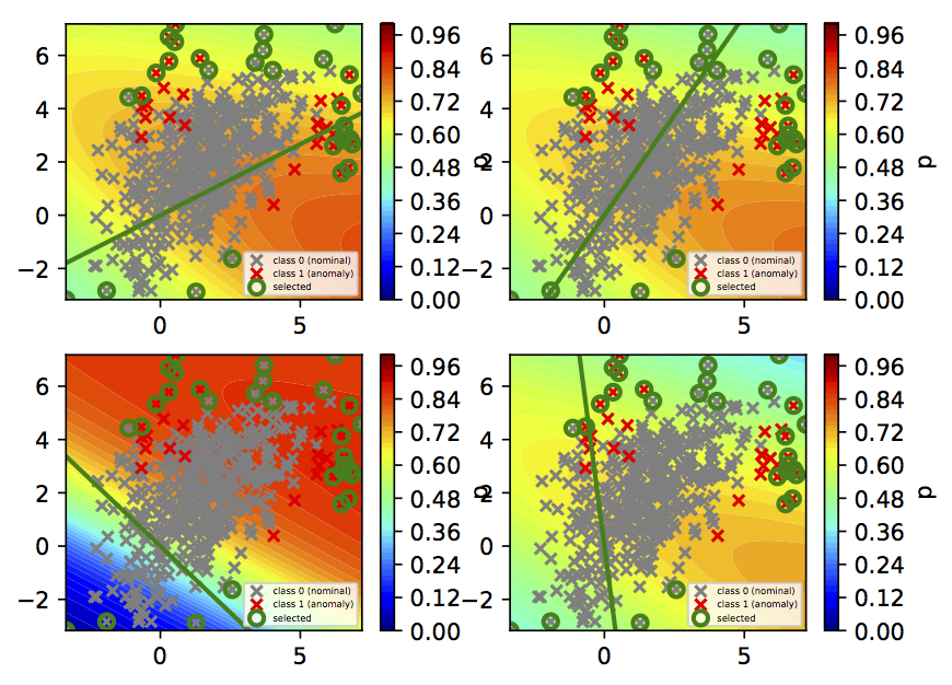
(d) Relevance after 30 feedback iterations

Figure 12: Toy data. More red on the top row indicates more anomalous. More red on the bottom row indicates more relevant. The red ‘$\times$’ are true anomalies and grey ‘$\times$’ are true nominals. (a) LODA with four projections (green lines) applied to the Toy dataset. (b) The contours of only the bottom left LODA projection are somewhat aligned with the true anomalies, i.e., most anomalies lie in the higher anomaly score regions. Other projections are highly inaccurate. (c) The learned anomaly scores output by GLAD after 30 feedback iterations. (d) The points circled in green were shown to the analyst for labeling, one per feedback iteration. After $30$ feedback iterations, the bottom left projection was found to be most relevant in the top-right half-space, whereas it is completely irrelevant in the bottom-left half-space. Other projections were less relevant in most parts of the feature space.

GLAD vs. Tree-based AAD. We may consider GLAD as very similar to the Tree-based AAD approach. Tree-based AAD method partitions the input feature space into discrete subspaces and then places a uniform prior over those subspaces (i.e., the uniform weight vector to combine ensemble scores). If we take this view to an extreme by imagining that each instance in the feature space represents a subspace, we can see the connection to GLAD. While Tree-based AAD assigns the scores of discrete subspaces to instances (e.g., node depths for Isolation Forest), the scores assigned by GLAD are continuous, defined by the global ensemble members. The relevance in GLAD is analogous to the learned weights in Tree-based AAD. This similarity lets us extend the key insight behind active learning with tree-based models (Section 4) to GLAD as well: uniform prior over weights of each subspace (leaf node) in Tree-based AAD and uniform prior over input feature space for the relevance of each ensemble member in GLAD are highly beneficial for label-efficient active learning. On the basis of this argument and its supporting empirical evidence, we claim that the following hypothesis is true:

Under an uniform prior on the detectors’ relevance over the input space, the greedy query selection strategy is label-efficient for active learning with any ensemble of pre-trained anomaly detectors.

Broader Applicability of the Key Idea behind GLAD. In practice, we often do not have control over the ensemble members. For example, the ensemble might have only a limited number of detectors. In the extreme case, there might only be a single pre-trained detector which cannot be modified. A scoring model that combines detector scores linearly would then lack capacity if the number of labeled instances (obtained through feedback) is high. In this case, GLAD can increase the capacity for incorporating feedback through the FSSN. The FSSN allows us to place a uniform prior over the input space. This property can be employed for domain adaptation of not only anomaly detector ensembles, but also other algorithms including classifier ensembles after they are deployed.

GLAD employs the AAD loss (Equation 11) for ranking scores relative to $q_{\tau}$ and ${\bf x}_{\tau}$ in a more general manner when compared to the linear scoring function. This technique can be applied more generally to any parameterized non-ensemble detector as well (such as the one based on density estimation) for both semi-supervised and active learning settings.

6.2 Explanations for Anomalies with GLAD

To help the analyst understand the results of active anomaly detection system, we have used the concept of “descriptions” for the tree-based ensembles. We now introduce the concept of “explanations” in the context of GLAD algorithm. While both descriptions and explanations seem similar, they are actually quite different:

• Description: A description generates a compact representation for a group of instances. The main application is to reduce the cognitive burden on the analysts while providing labeling feedback for queried instances.

• Explanation: An explanation outputs a reason why a specific data instance was assigned a high anomaly score. Generally, we limit the scope of an explanation to one data instance. The main application is to diagnose the model: whether the anomaly detector(s) are working as expected or not.

GLAD assumes that the anomaly detectors in the ensemble can be arbitrary (homogeneous or heterogeneous). The best it can offer as an explanation is to output the member which is most relevant for a test data instance. With this in mind, we can employ the following approach to generate explanations:

1. Employ the FSSN network to predict the relevance of individual ensemble members on the complete dataset. It is important to note that the relevance of a detector is different from the anomaly score(s) it assigns. A detector which is relevant in a particular subspace predicts the labels of instances in that subspace correctly irrespective of whether those instances are anomalies or nominals.

2. Find the instances for each ensemble member for which that detector is the most relevant. Mark these instances as positive and the rest as negative.

3. Train a separate decision tree for each member to separate the corresponding positives and negatives. This describes the subspaces where each ensemble member is relevant. Figure 13 illustrates this idea on the Toy dataset.

4. When asked to explain the anomaly score for a given test instance:

   1. Use FSSN network to identify the most relevant ensemble member for the test instance.

   2. Employ a model agnostic explanation technique such as LIME (?) or ANCHOR (?) to generate the explanation using the most relevant ensemble member. As a simple illustration, we trained GLAD on the synthetic dataset and a LODA ensemble with four projections. After $30$ feedback iterations, the unlabeled instance at $(6.12,3.04)$ had the highest anomaly score. We used LIME to explain its anomaly score. LIME explanation is shown below:

      ΨΨ(’2.16 < y <= 3.31’, -0.4253860500153764)
      ΨΨ(’x > 2.65’, 0.3406543313093905)
      ΨΨ
      

      Here the explanation 2.16 < y <= 3.31 from member $2$ has the highest absolute weight and hence, explains most of the anomaly score.

Since most aspects of explanations are qualitative, we leave their evaluation on real-world data to future work.

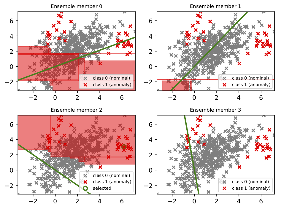
(a)

Figure 13: Most relevant ensemble members in subspaces inferred with GLAD after 30 feedback iterations. There are four members (i.e., LODA projections) in our current example. The region where a member is ranked as the top-most relevant detector is shown in red. Note that members 0 and 1 were found relevant in subspaces which have mostly nominal instances. This is because they correctly assigned low anomaly scores to instances in those subspaces. The last member (member 3) did not rank as the top-most relevant detector for any instance; hence, it does not have any region marked in red. The point circled in green (in bottom left plot) is a test instance. Ensemble member 2 was found to be the most relevant for this instance.

7 Experiments and Results

Table 1: Description of benchmark datasets used in our experiments.

Dataset	Nominal Class	Anomaly Class	Total	Dims	# Anomalies(%)
Abalone	8, 9, 10	3, 21	1920	9	29 (1.5%)
ANN-Thyroid-1v3	3	1	3251	21	73 (2.25%)
Cardiotocography	1 (Normal)	3 (Pathological)	1700	22	45 (2.65%)
Covtype	2	4	286048	54	2747 (0.9%)
KDD-Cup-99	‘normal’	‘u2r’, ‘probe’	63009	91	2416 (3.83%)
Mammography	-1	+1	11183	6	260 (2.32%)
Shuttle	1	2, 3, 5, 6, 7	12345	9	867 (7.02%)
Yeast	CYT, NUC, MIT	ERL, POX, VAC	1191	8	55 (4.6%)
Electricity	DOWN	UP	27447	13	1372 (5%)
Weather	No Rain	Rain	13117	8	656 (5%)

Datasets. We evaluate our algorithms on ten publicly available benchmark datasets ((?),(?),(?), UCI(?)) listed in Table 1. The anomaly classes in Electricity and Weather were down-sampled to be 5% of the total.

Evaluation Methodology. For each variant of the algorithm, we plot the percentage of the total number of anomalies shown to the analyst versus the number of instances queried; this is the most relevant metric for an analyst in any real-world application. Higher plot means the algorithm is better in terms of discovering anomalies. All results presented are averaged over 10 different runs and the error-bars represent $95\%$ confidence intervals.

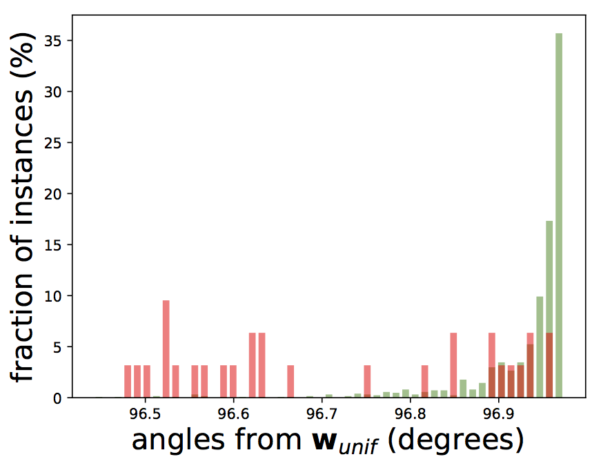
(a) Abalone

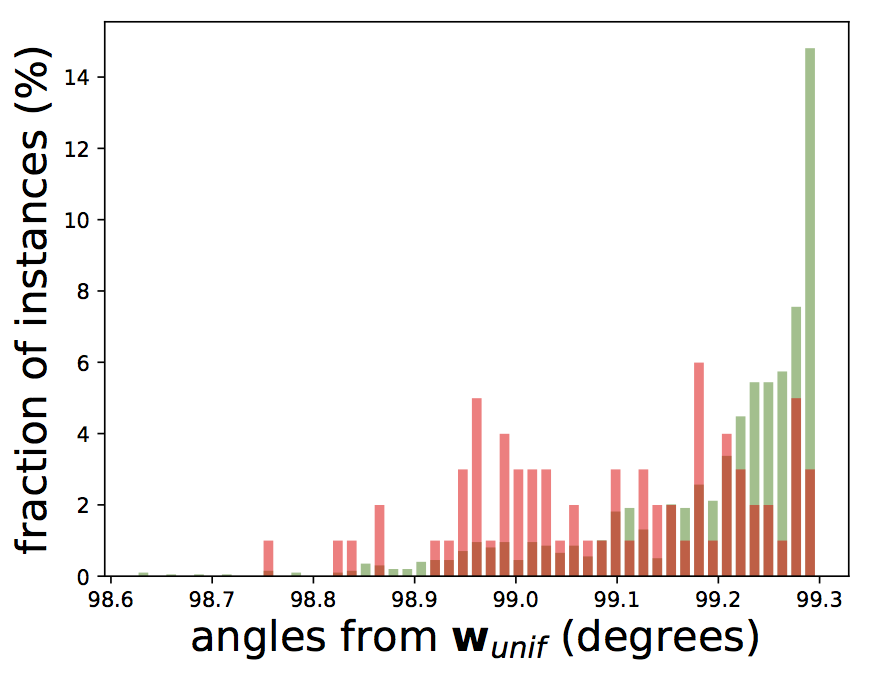
(b) ANN-Thyroid

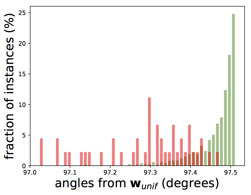
(c) Cardiotocography

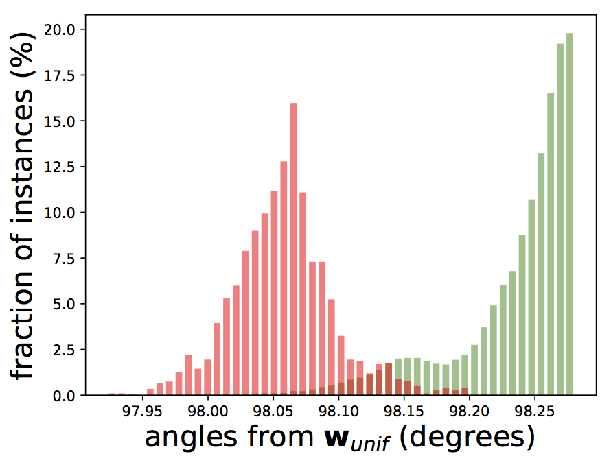
(d) Covtype

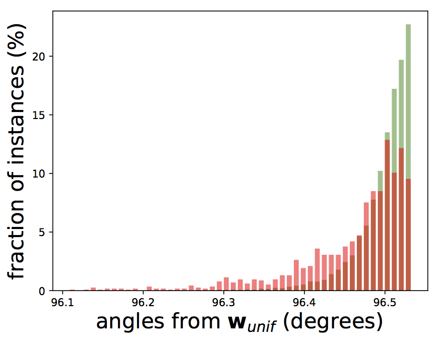
(e) Electricity

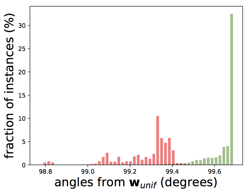
(f) KDDCup99

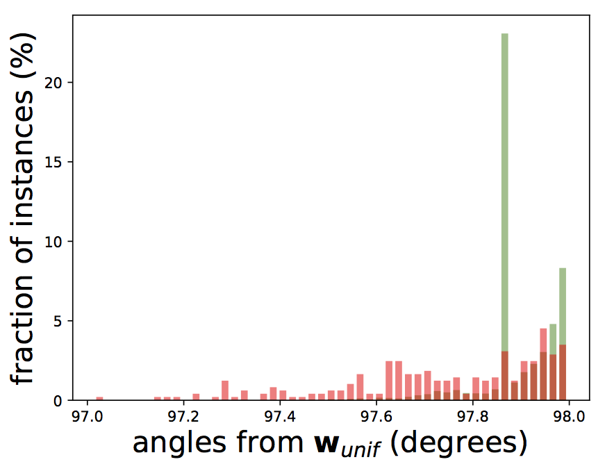
(g) Mammography

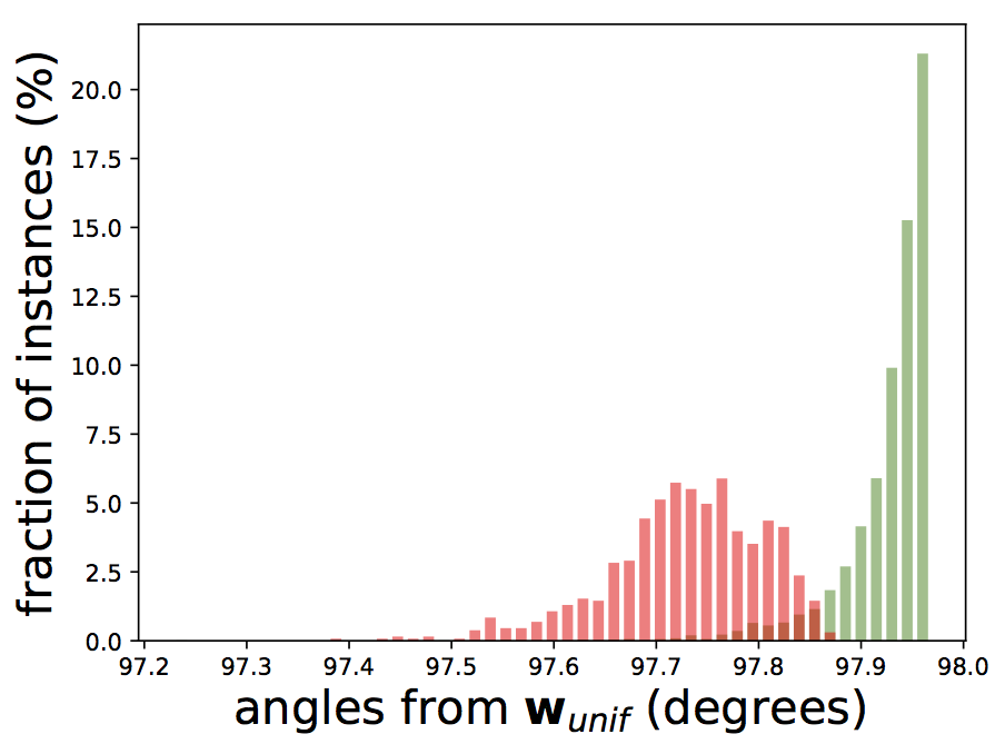
(h) Shuttle

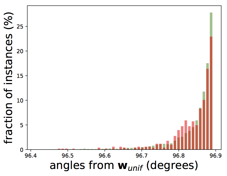
(i) Weather

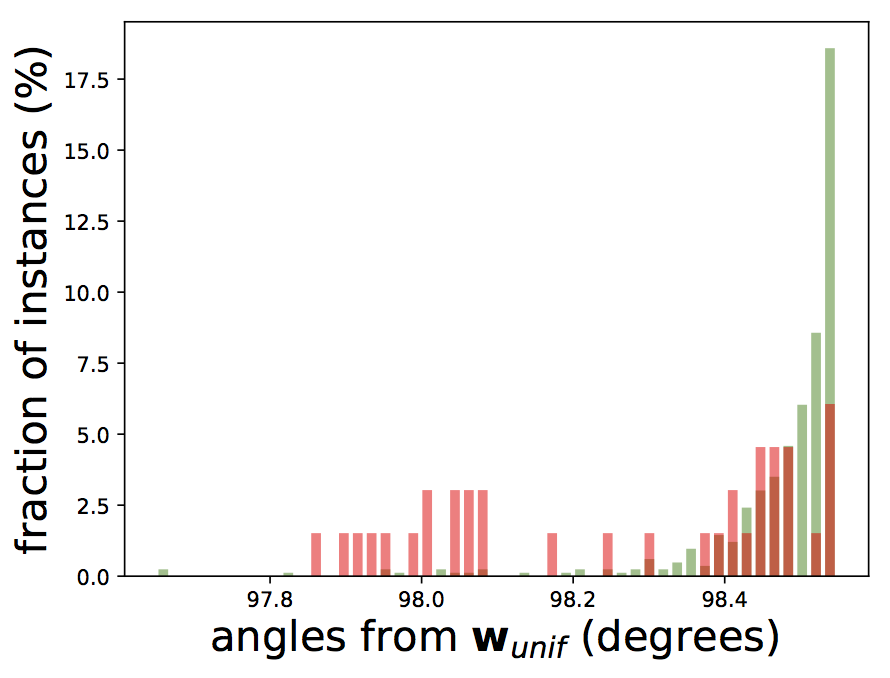
(j) Yeast

Figure 14: Histogram distribution of the angles between score vectors from IFOR and ${\mathbf{w}}_{unif}$ for all datasets. The red and green histograms show the angle distributions for anomalies and nominals respectively. Since the red histograms are closer to the left, anomalies are aligned closer to ${\mathbf{w}}_{unif}$.

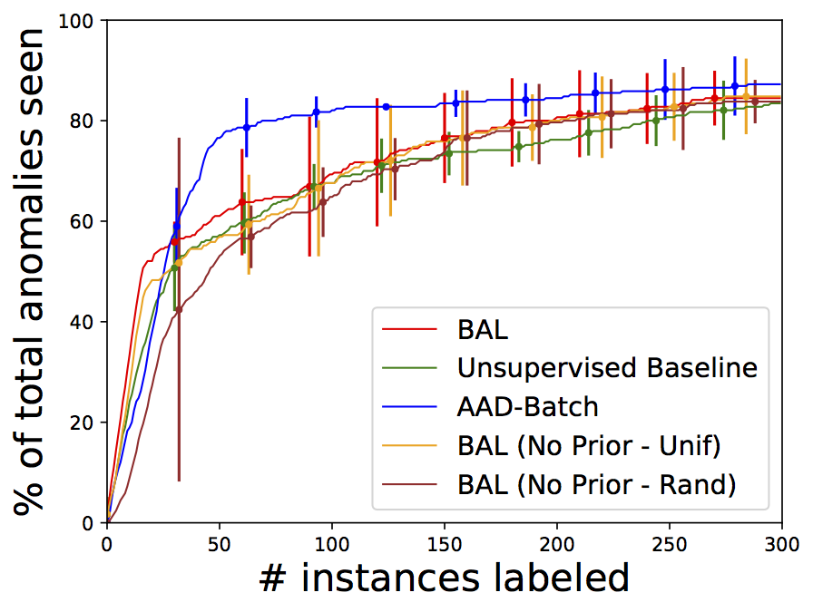
(a) Abalone

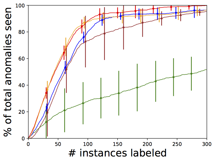
(b) ANN-Thyroid-1v3

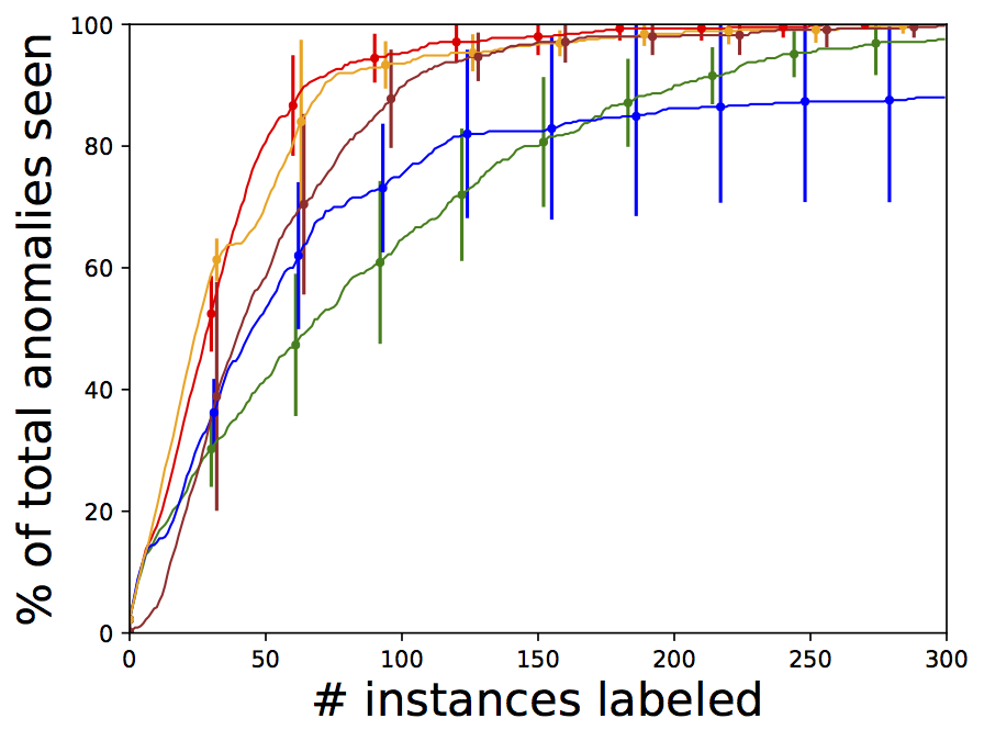
(c) Cardiotocography

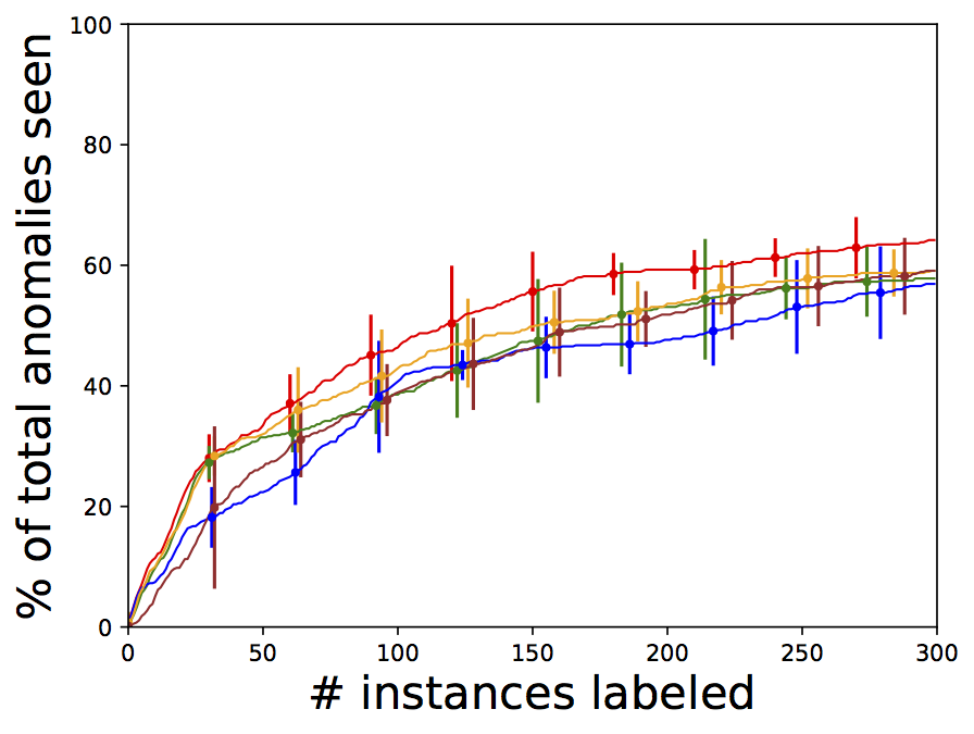
(d) Yeast

Figure 15: Percentage of total anomalies seen vs. the number of queries for the smaller datasets in the batch setting.

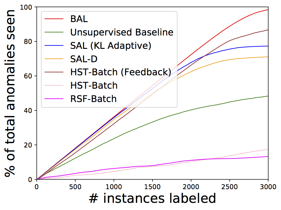
(a) Covtype

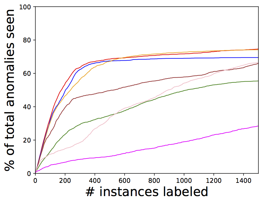
(b) Mammography

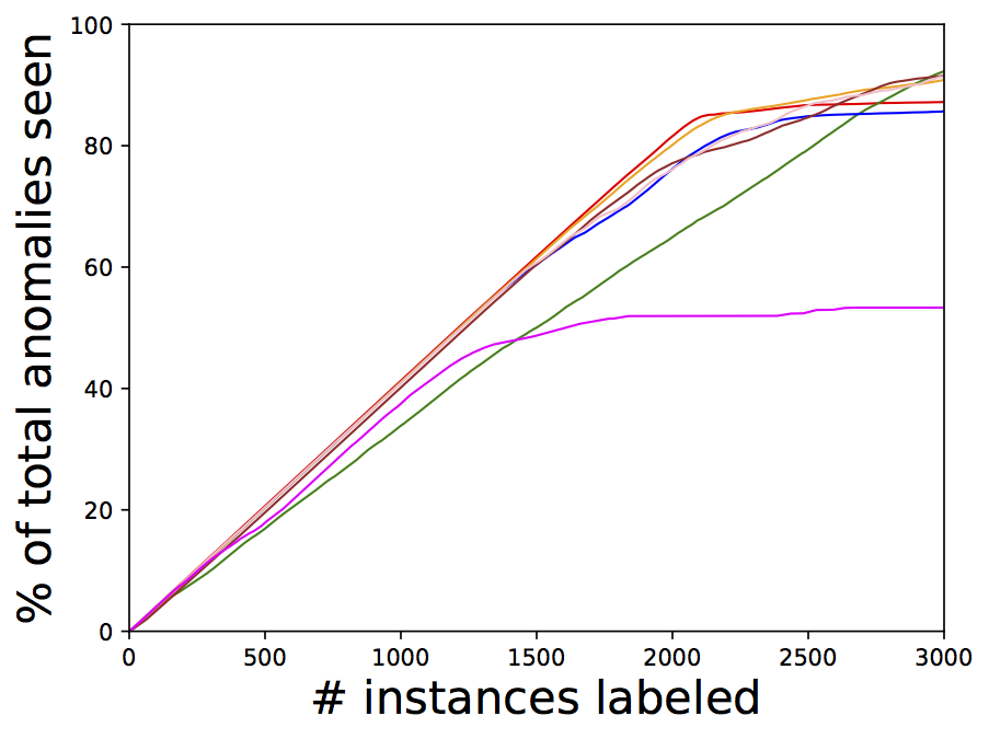
(c) KDD-Cup-99

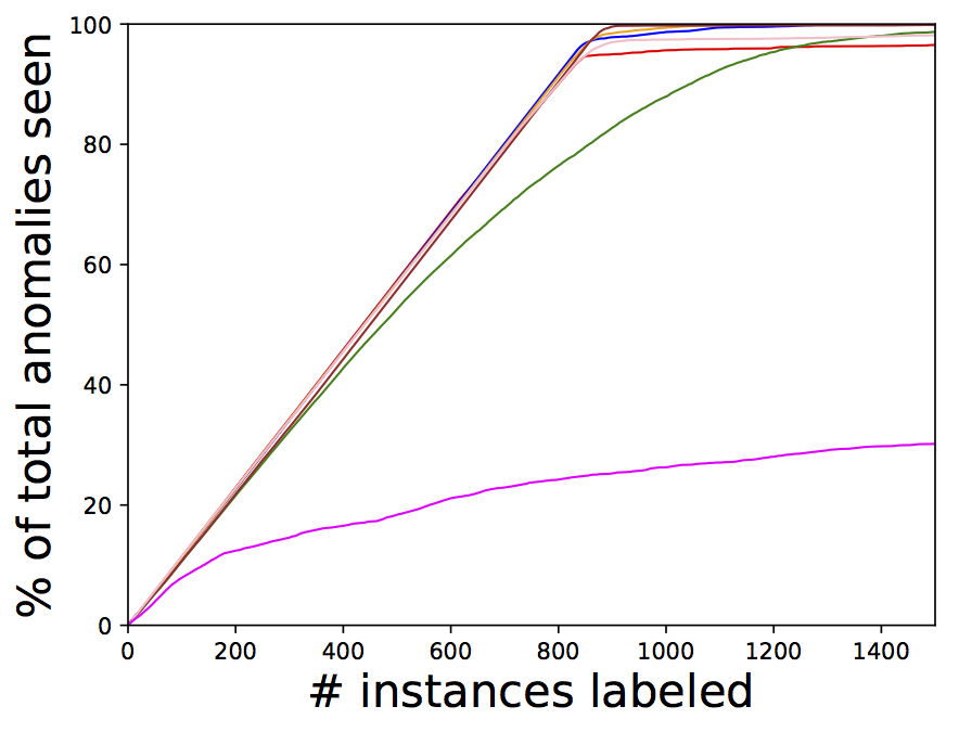
(d) Shuttle

Figure 16: Percentage of total anomalies seen vs. number of queries for the larger datasets in the limited memory setting. SAL (KL Adaptive) and SAL-D apply the Select-Top and Select-Diverse query strategies resp. Mammography, KDD-Cup-99, and Shuttle have no significant drift. Covtype, which has a higher drift, is included here for comparison because it is large.

7.1 Results for Active Anomaly Detection with Tree Ensembles

Experimental Setup. All versions of Batch Active Learning (BAL) and Streaming Active Learning (SAL) employ IFOR with the number of trees $T=100$ and subsample size $256$. The initial starting weights are denoted by ${\bf w}^{(0)}$. We normalize the score vector for each instance to unit length such that the score vectors lie on a unit sphere. This normalization helps adhere to the discussion in Section 4, but is otherwise unnecessary. Figure 14 shows that ${\mathbf{w}}_{unif}$ tends to have a smaller angular separation from the normalized IFOR score vectors of anomalies than from those of nominals. This holds true for most of our datasets (Table 1). Weather is a hard dataset for all anomaly detectors (?), as reflected in its angular distribution in Figure 14i. In all our experiments, Unsupervised Baseline shows the number of anomalies detected without any feedback, i.e., using the uniform ensemble weights ${\mathbf{w}}_{unif}$; BAL (No Prior - Unif) and BAL (No Prior - Rand) impose no priors on the model, and start active learning with ${\mathbf{w}}^{(0)}$ set to ${\mathbf{w}}_{unif}$ and a random vector respectively; BAL sets ${\mathbf{w}}_{unif}$ as prior, and starts with ${\mathbf{w}}^{(0)}={\mathbf{w}}_{unif}$. For HST, we present two sets of results with batch input only: HST-Batch with original settings ($T=25$, depth=$15$, no feedback) (?), and HST-Batch (Feedback) which supports feedback with BAL strategy (with $T=50$ and depth=$8$, a better setting for feedback). For RST, we present the results (RST-Batch) with only the original settings ($T=30$, depth=$15$) (?) since it was not competitive with other methods on our datasets. We also compare the BAL variants with the AAD approach (?) in the batch setting (AAD-Batch). Batch data setting is the most optimistic for all algorithms.

7.1.1 Results for Diversified Query Strategy

The diversified querying strategy Select-Diverse (Algorithm 1) employs compact descriptions to select instances. Therefore, the evaluation of its effectiveness is presented first. An interactive system can potentially ease the cognitive burden on the analysts by using descriptions to generate a “summary” of the anomalous instances.

We perform a post hoc analysis on the datasets with the knowledge of the original classes (Table 1). It is assumed that each class in a dataset represents a different data-generating process. To measure the diversity at any point in our feedback cycle, we compute the difference between the number of unique classes presented to the analyst per query batch averaged across all the past batches. The parameter $\delta$ for Select-Diverse was set to $5$ in all experiments. We compare three query strategies in the batch data setup: BAL-T, BAL-D, and BAL-R. BAL-T simply presents the top three most anomalous instances per query batch. BAL-D employs Select-Diverse to present three diverse instances out of the ten most anomalous instances. BAL-R presents three instances selected at random from the top ten anomalous instances. Finally, BAL greedily presents only the single most anomalous instance for labeling. We find that BAL-D presents a more diverse set of instances than both BAL-T (solid lines) as well as BAL-R (dashed lines) on most datasets. Figure 17b shows that the number of anomalies discovered (on representative datasets) with the diversified querying strategy is similar to the greedy strategy, i.e., no loss in anomaly discovery rate to improve diversity. The streaming data variants SAL-* have similar performance as the BAL-* variants.

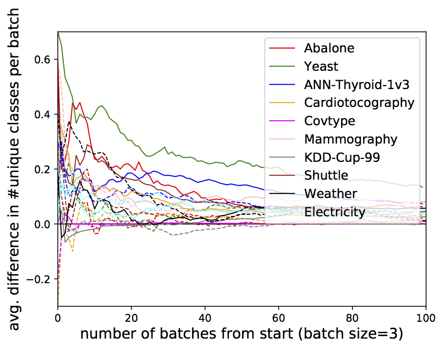
(a) Class diversity

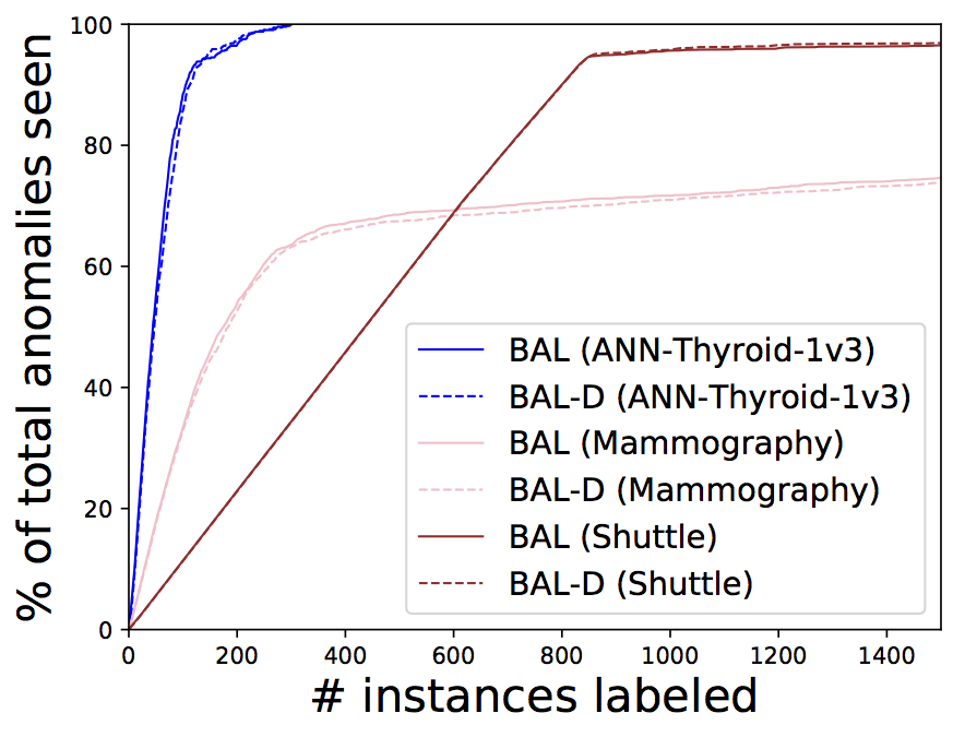
(b) % anomalies seen

Figure 17: Results comparing diversified querying strategy textttBAL-D with baseline query strategies BAL-T and BAL-R. The x-axis in (a) shows the number of query batches (of batch size 3). The y-axis shows the difference in the number of unique classes seen averaged across all batches till a particular batch. The solid lines in (a) show the average difference between unique classes seen with BAL-D and BAL-T; the dashed lines show the average difference between BAL-D and BAL-R.

7.1.2 Results for Anomaly Descriptions with Interpretability

We compare the Compact Descriptions (CD) for interpretability (Algorithm 2) with Bayesian Rulesets (BR) in Figure 18. Our experimental setup for active learning is transductive (i.e., learning is performed over the combined set of labeled and unlabeled instances) and the number of anomalies is very small. Therefore, we compute precision, recall, and F1 metrics of the learned model over the combined dataset with ground-truth labels after each feedback cycle. It is hard to present a qualitative comparison between them since they both have similar F1 Scores. BR has higher precision whereas CD has higher recall in general. However, CD usually generates rules of smaller lengths than BR. Some rule sets generated for Abalone and Yeast are presented in Appendix A. CD often generates more number of simpler rules that define “anomalies”. Therefore, their recall is higher. This is particularly pronounced for Yeast (Table 4 and Table 5). Prior work (?) suggests that this attribute might be advantageous to end users. However, the judgment of description quality is subjective and dependent on the specific dataset and application.

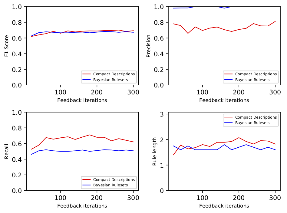
(a) Abalone

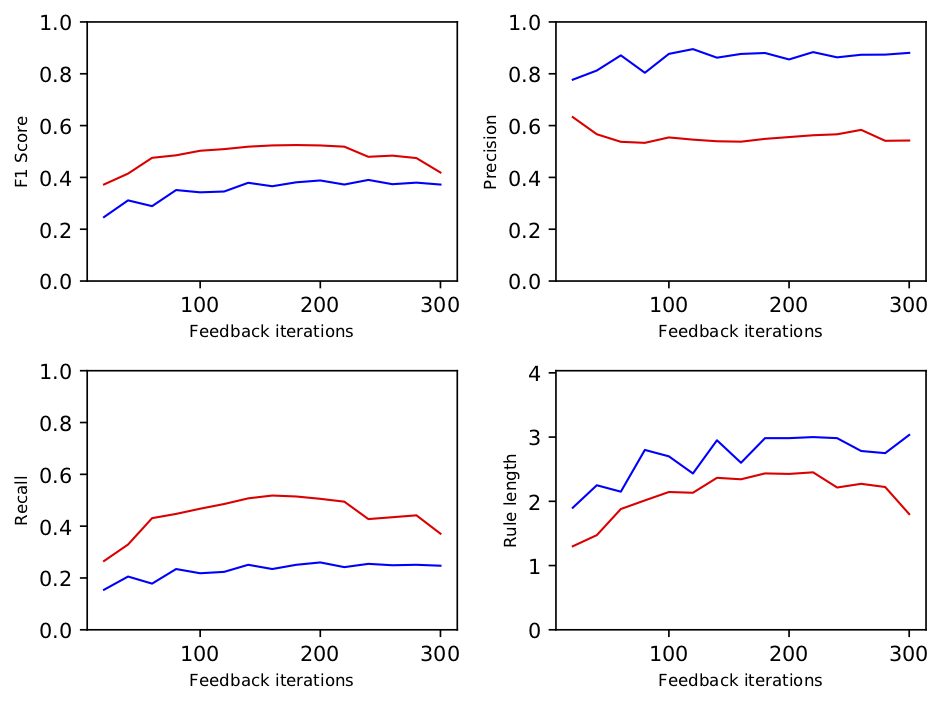
(b) Yeast

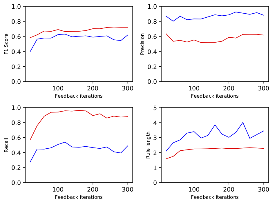
(c) Cardiotocography

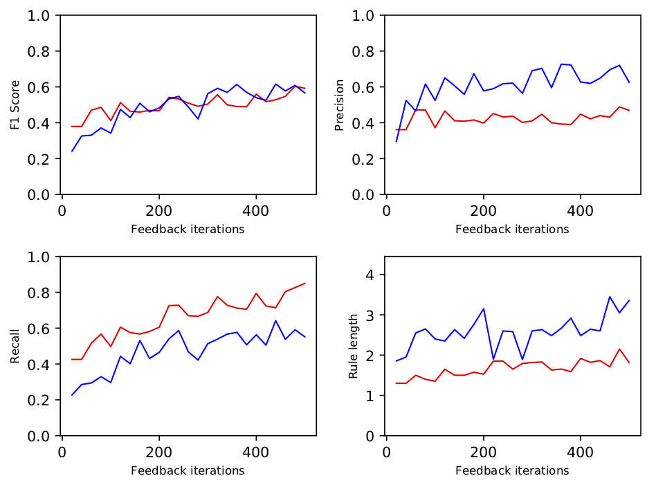
(d) Covtype

Figure 18: Results comparing Compact Descriptions (CD) with Bayesian Rulesets (BR) (?) on representative datasets. The result for each dataset has four sets of plots: F1 Score, Precision, Recall, and Rule length.

7.1.3 Results for Batch Active Learning (BAL)

We set the budget $B$ to $300$ for all datasets in the batch setting. The results on the four smaller datasets Abalone, ANN-Thyroid-1v3, Cardiotocography, and Yeast are shown in Figure 15. The performance is similar for the larger datasets as shown in Figure 16. When the algorithm starts from sub-optimal initialization of the weights and with no prior knowledge (BAL (No Prior - Rand)), more number of queries are spent hunting for the first few anomalies, and thereafter detection improves significantly. When the weights are initialized to ${\mathbf{w}}_{unif}$, which is a reliable starting point (BAL (No Prior - Unif) and BAL), fewer queries are required to find the initial anomalies, and typically results in a lower variance in accuracy. Setting ${\mathbf{w}}_{unif}$ as prior in addition to informed initialization (BAL) performs better than without the prior (BAL (No Prior - Unif)) on Abalone, ANN-Thyroid-1v3, and Yeast. We believe this is because the prior helps guard against noise.

7.1.4 Results for Streaming Active Learning (SAL)

In all SAL experiments, we set the number of queries per window $Q=20$. The total budget $B$ and the stream window size $K$ for the datasets were set respectively as follows: Covtype (3000, 4096), KDD-Cup-99 (3000, 4096), Mammography (1500, 4096), Shuttle (1500, 4096), Electricity (1500, 1024), Weather (1000, 1024). These values are reasonable w.r.t the dataset’s size, the number of anomalies, and the rate of concept drift. The maximum number of unlabeled instances residing in memory is $K$. When the last window of data arrives, then active learning is continued with the final set of unlabeled data retained in the memory until the total budget $B$ is exhausted. The instances are streamed in the same order as they appear in the original public sources. When a new window of data arrives: SAL (KL Adaptive) dynamically determines which trees to replace based on KL-divergence, SAL (Replace $20\%$ Trees) replaces $20\%$ oldest trees, and SAL (No Tree Replace) creates the trees only once with the first window of data and only updates the weights of the fixed leaf nodes with feedback thereafter.

Limited memory setting with no concept drift. The results on the four larger datasets are shown in Figure 16. The performance is similar to what is seen on the smaller datasets. Among the unsupervised algorithms in the batch setting, IFOR (Unsupervised Baseline) and HST (HST-Batch) are competitive, and both are better than RSF (RSF-Batch). With feedback, BAL is consistently the best performer. HST with feedback (HST-Batch (Feedback)) always performs better than HST-Batch. The streaming algorithm with feedback, SAL (KL Adaptive), significantly outperforms Unsupervised Baseline and is competitive with BAL. SAL (KL Adaptive) performs better than HST-Batch (Feedback) as well. SAL-D which presents a more diverse set of instances for labeling performs similar to SAL (KL Adaptive). These results demonstrate that the feedback-tuned anomaly detectors generalize to unseen data.

Figure 20 shows drift detection on datasets which do not have any drift. The streaming window size for each dataset was set commensurate to its total size: Abalone($512$), ANN-Thyroid-1v3($512$), Cardiotocography($512$), Covtype($4096$), Electricity($1024$), KDDCup99($4096$), Mammography($4096$), Shuttle($4096$), Weather($1024$), and Yeast($512$).

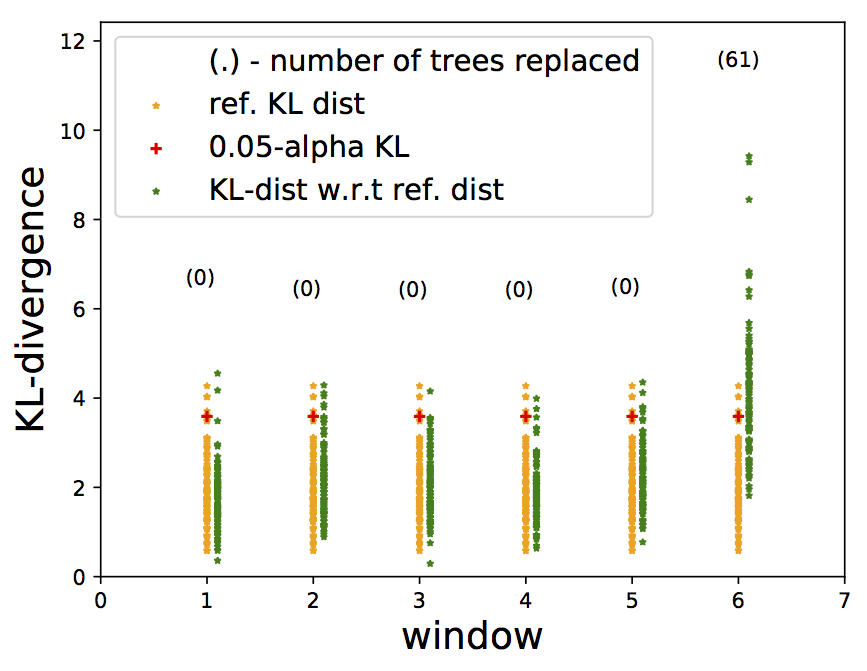
(a) ANN-Thyroid-1v3

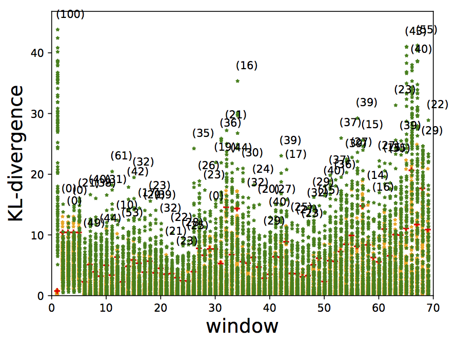
(b) Covtype

Figure 19: Results for drift detection across windows. (a) When there is no drift, such as in ANN-Thyroid-1v3, then no trees are replaced for most of the windows, and the older model is retained. (b) If there is drift, such as in Covtype, then the trees are more likely to be replaced.

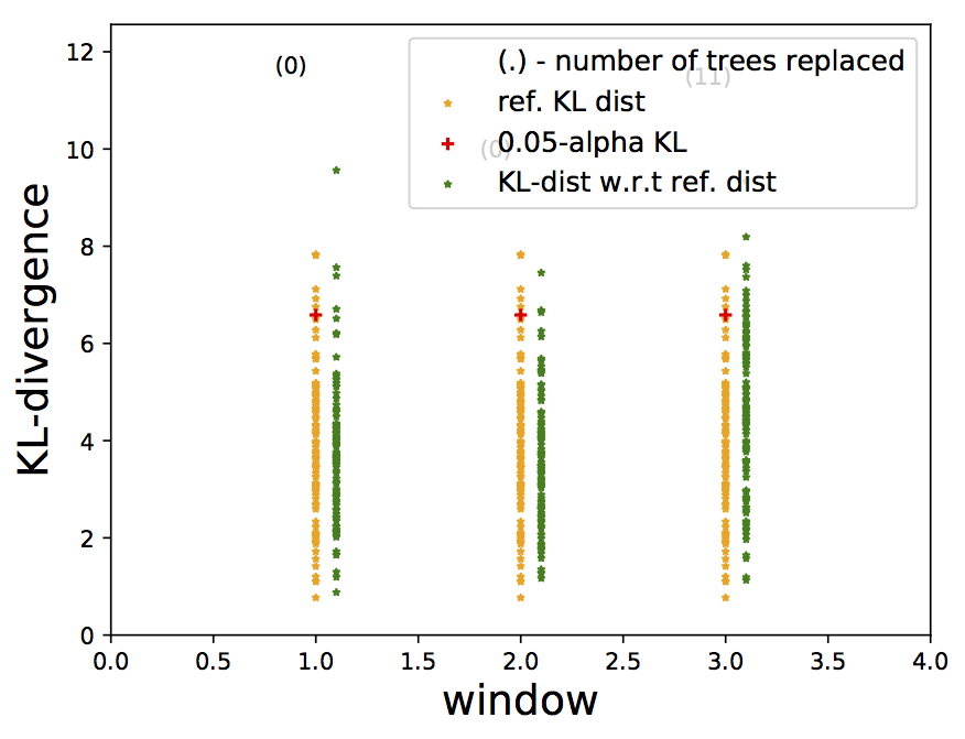
(a) Abalone

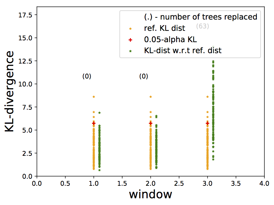
(b) Cardiotocography

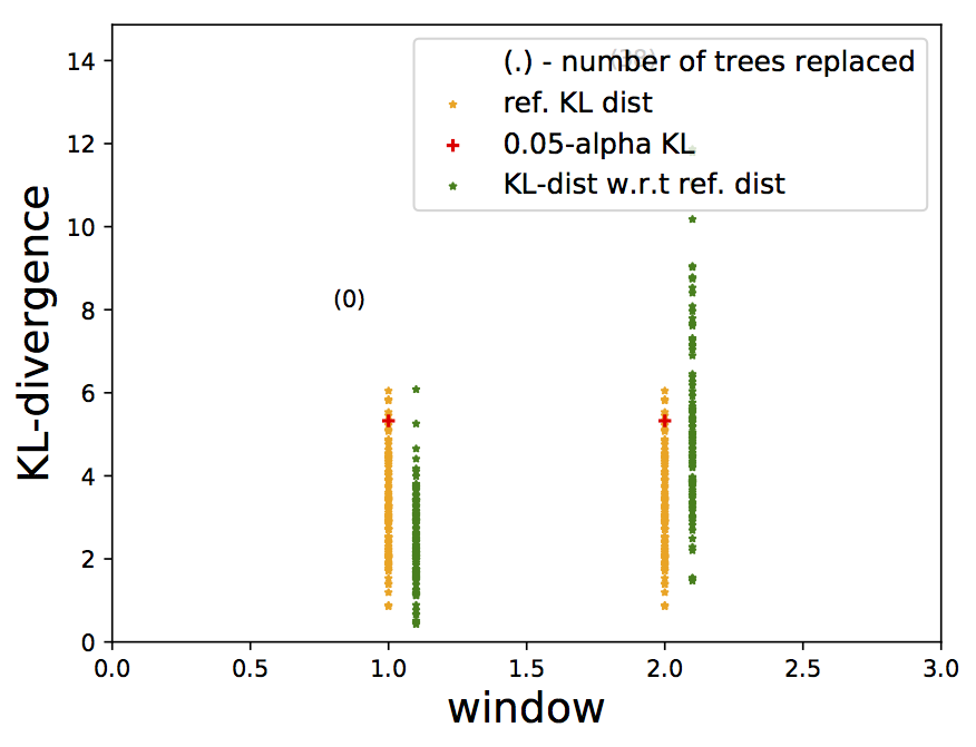
(c) Yeast

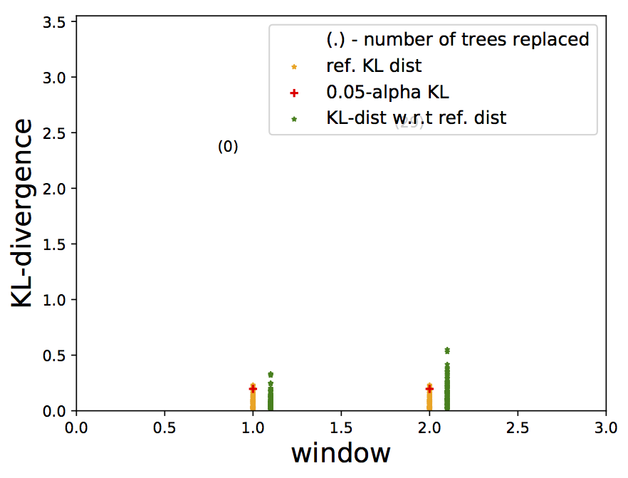
(d) Mammography

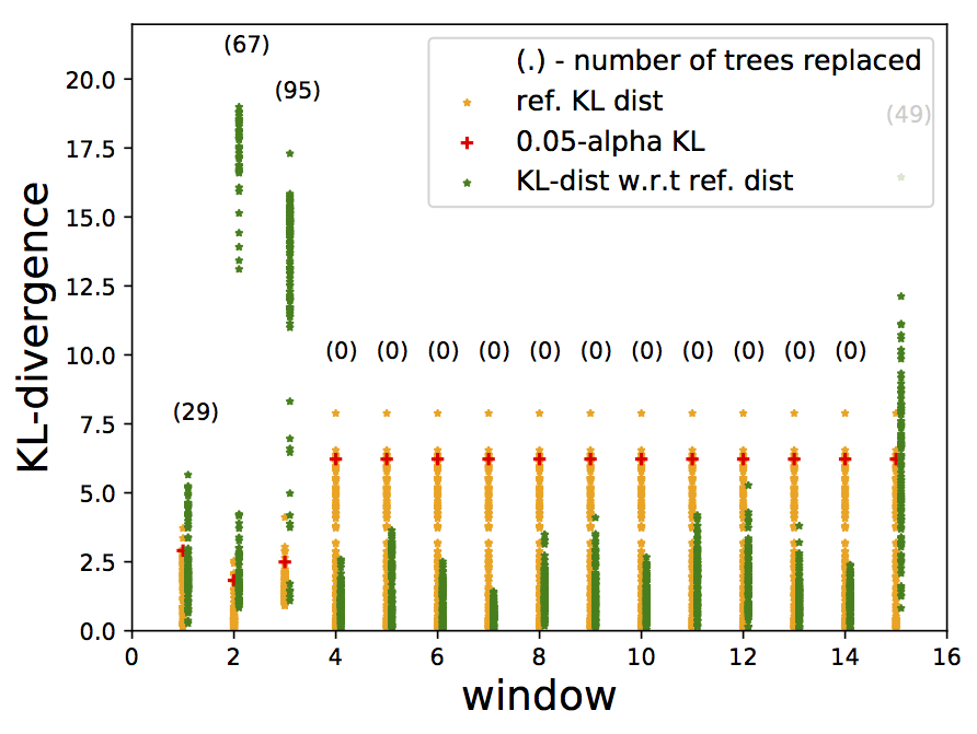
(e) KDD-Cup-99

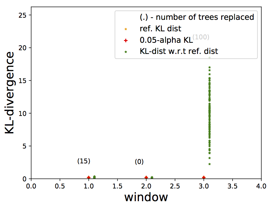
(f) Shuttle

Figure 20: The last data window in each dataset usually has much fewer instances and therefore, its distribution is very different from the previous window despite there being no data drift. Therefore, we ignore the drift in the last window. We did not expect Abalone, Cardiotocography, KDDCup99, Mammography, Shuttle, Yeast, and ANN-Thyroid-1v3 (Figure 19a) to have much drift in the data. This can also be seen in the plots where most of the windows in the middle of streaming did not result in too many trees being replaced (the numbers in the parenthesis are mostly zero).

Streaming setting with concept drift. Figure 21 shows the results after integrating drift detection and label feedback with SAL for the datasets which are expected to have significant drift. Both Covtype and Electricity show more drift in the data than Weather (top row in Figure 21). The rate of drift determines how fast the model should be updated. If we update the model too fast, then we loose valuable knowledge gained from feedback which is still valid. On the other hand, if we update the model too slowly, then the model continues to focus on the stale subspaces based on the past feedback. It is hard to find a common rate of update that works well across all datasets (such as replacing $20\%$ trees with each new window of data). Figure 21 (bottom row) shows that the adaptive strategy (SAL (KL Adaptive)) which replaces obsolete trees using KL-divergence, as illustrated in Figure 21 (top row), is robust and competitive with the best possible configuration, i.e., BAL.

(a) Covtype

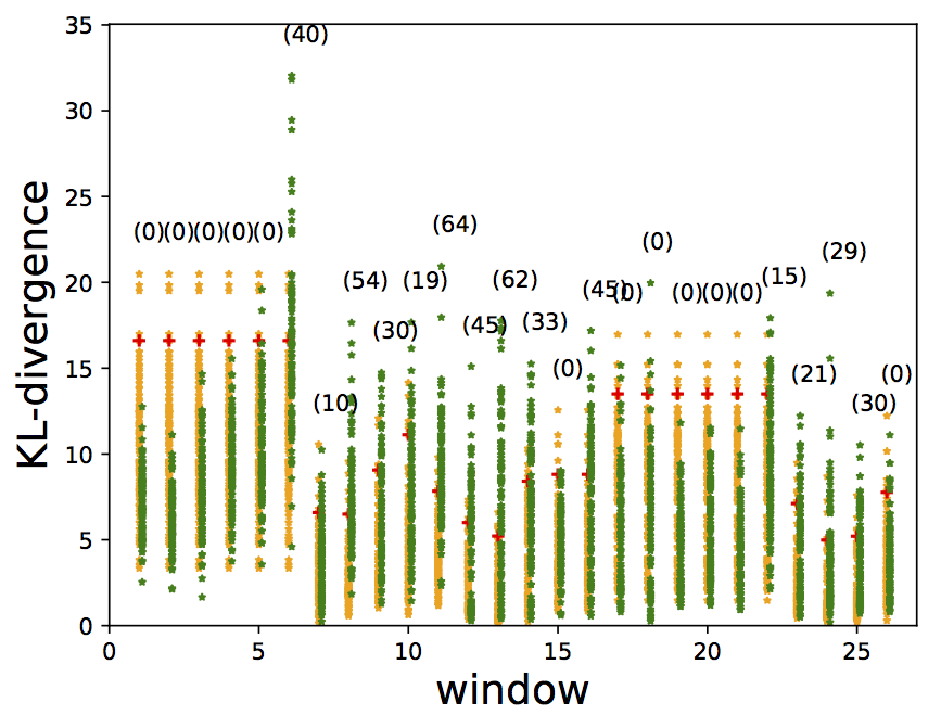
(b) Electricity

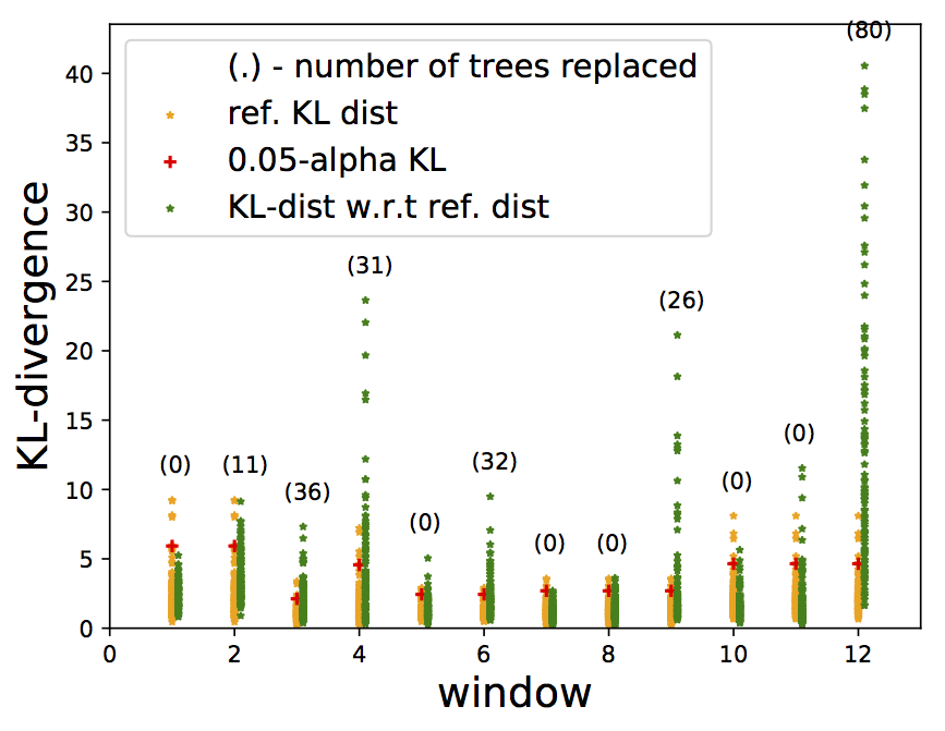
(c) Weather

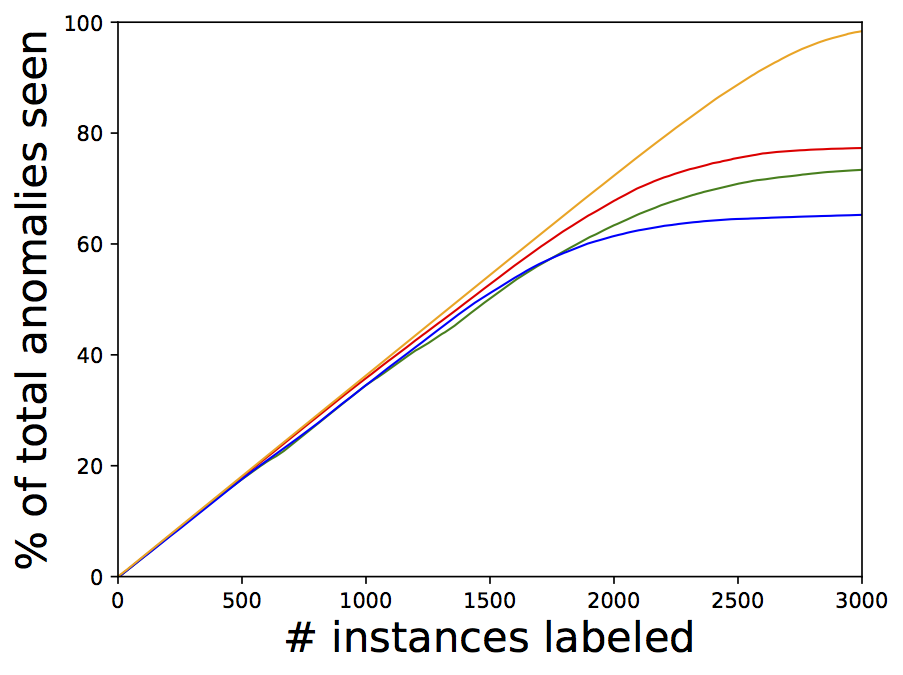
(d) Covtype

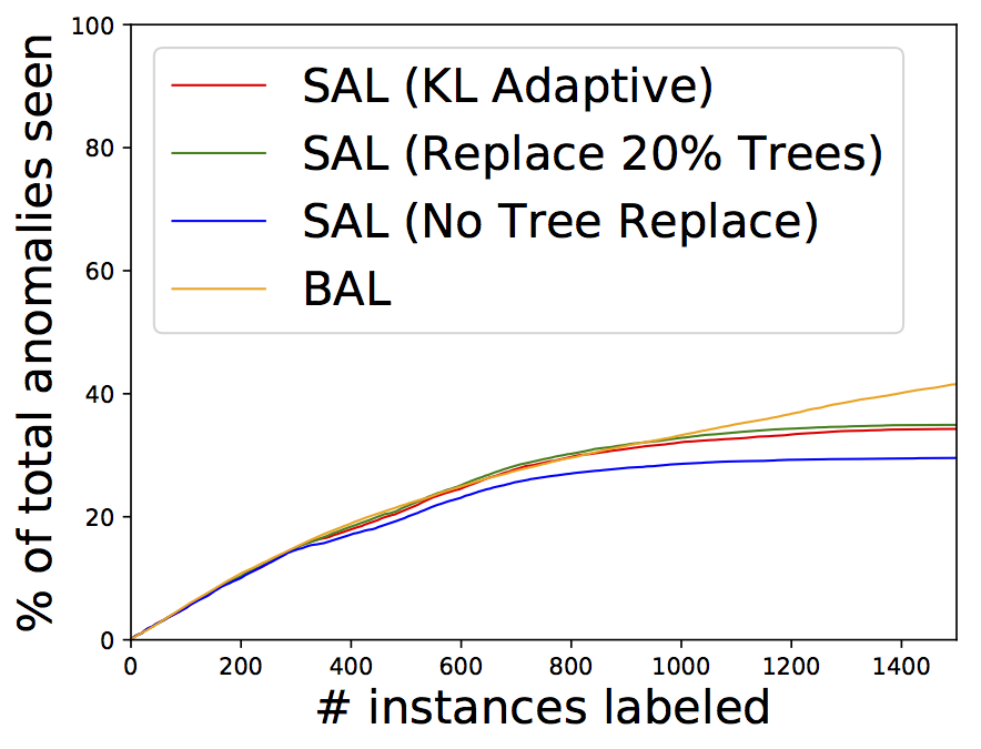
(e) Electricity

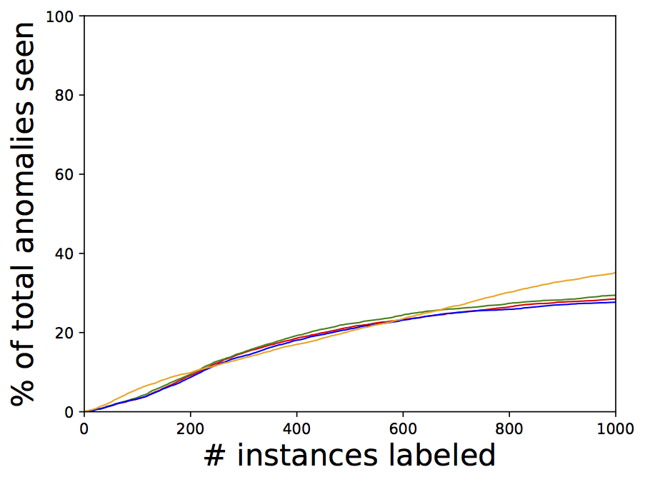
(f) Weather

Figure 21: Results for integrated drift detection and label feedback with Streaming Active Learning (SAL) algorithm. The top row shows the number of trees replaced per window when a drift in the data was detected relative to previous window(s). The bottom row shows the percentage of total anomalies seen vs. number of queries for the streaming datasets with significant concept drift.

7.2 Results for Active Anomaly Detection with GLAD Algorithm

In this section, we evaluate our GLocalized Anomaly Detection (GLAD) algorithm that is applicable for generic ensembles.

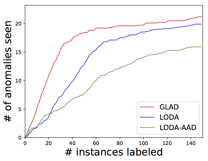
(a) Abalone

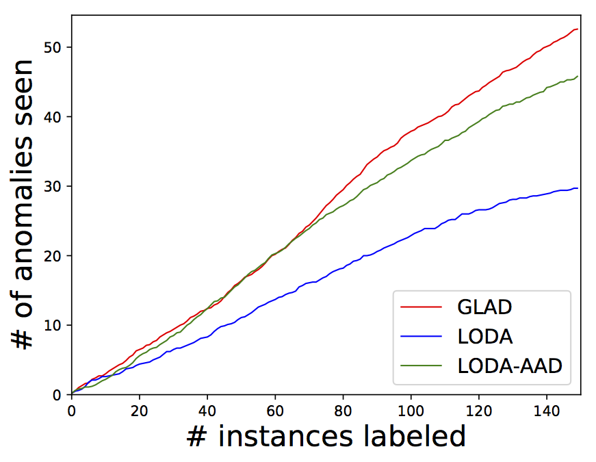
(b) ANN-Thyroid-1v3

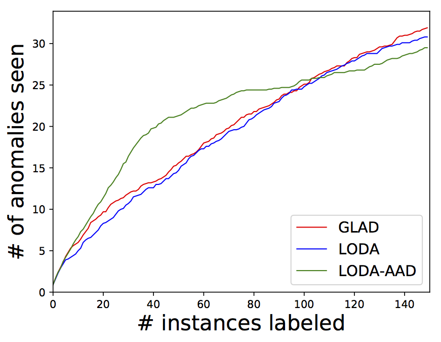
(c) Cardiotocography

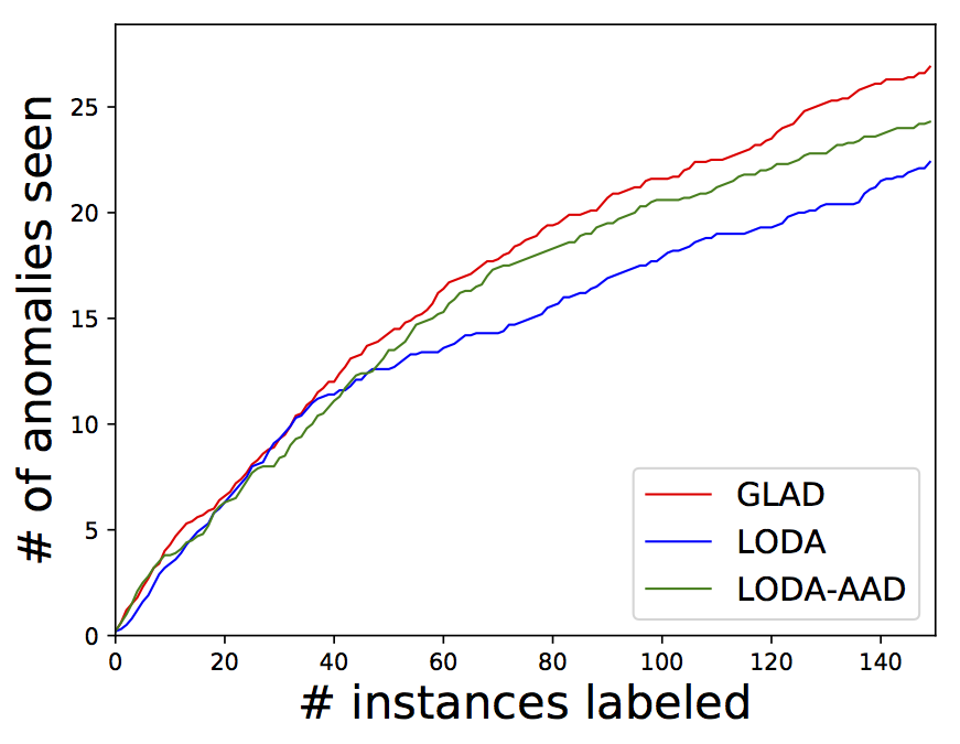
(d) Yeast

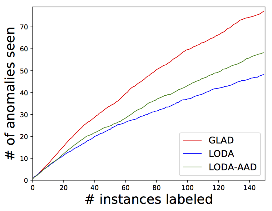
(e) Mammography

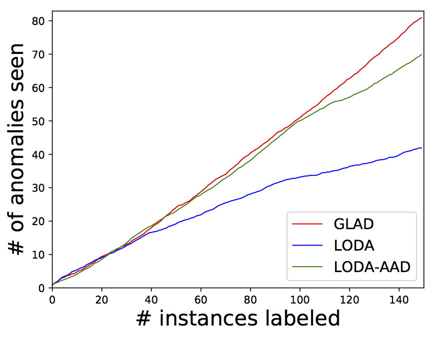
(f) KDD-Cup-99

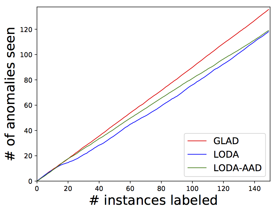
(g) Shuttle

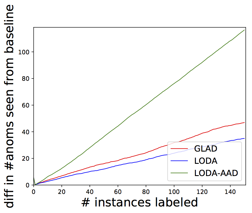
(h) Covtype

Figure 22: Results comparing GLAD with LODA and LODA-AAD on real-world datasets. Number of anomalies discovered as a function of the number of label queries. Results were averaged over $10$ different runs.

LODA based Anomaly Detector. For our anomaly detector, we employ the LODA algorithm (?), which is an ensemble ${\bf\mathcal{E}}=\{\mathcal{D}_{m}\}_{m=1}^{M}$ of $M$ one-dimensional histogram density estimators computed from sparse random projections. Each projection $\mathcal{D}_{m}$ is defined by a sparse $d$-dimensional random vector $\bf{\beta}_{m}$. LODA projects each data point onto the real line according to $\bf{\beta}_{m}^{\top}{\bf x}$ and then forms a histogram density estimator $f_{m}$. The anomaly score assigned to a given instance ${\bf x}$ is the mean negative log density: Score(${\bf x}$) = $\frac{1}{M}\sum_{m=1}^{M}{s_{m}({\bf x})}$, where, $s_{m}({\bf x})\triangleq-\log(f_{m}({\bf x}))$.

LODA gives equal weights to all projections. Since the projections are selected at random, every projection may not be good at isolating anomalies uniformly across the entire input feature space. LODA-AAD (?) was proposed to integrate label feedback from a human analyst by learning a better weight vector ${\bf w}$ that assigns weights proportional to the usefulness of the projections: weights are global, i.e., they are fixed across the entire input feature space. In contrast, we employ GLAD to learn the local relevance of each detector in the input space using the label feedback.

Feature Space Suppression Network (FSSN) Details. We employed a shallow neural network with $\max(50,3M)$ hidden nodes for all our test datasets, where $M$ is the number of ensemble members (i.e., LODA projections). The network is retrained after receiving each label feedback. During the retraining process, we cycle over the entire dataset (labeled and unlabeled) once. Since the labeled instances are very few, we up-sample the labeled data five times. We also employ $L2$-regularization for training the weights of the neural network.

Results on Real-world Data. We evaluate GLAD on all the benchmark datasets listed in Table 1. Since GLAD is most relevant when the anomaly detectors are specialized and fewer in number, we employ a LODA ensemble with a maximum of $15$ projections. Figure 22 shows the results comparing unsupervised LODA, LODA-AAD (weights the ensemble members globally) (?), and GLAD algorithms. We observe that GLAD outperforms both the baseline LODA as well as LODA-AAD. These results show the effectiveness of GLAD in learning the local relevance of ensemble members and discovering anomalies via label feedback.

7.3 Summary of Experimental Findings

We briefly summarize the main findings of our empirical evaluation.

• Uniform prior over the weights of the scoring function to rank data instances is very effective for active anomaly detection. The histogram distribution of the angles between score vectors from Isolation Forest (IFOR) and ${\mathbf{w}}_{unif}$ show that anomalies are aligned closer to ${\mathbf{w}}_{unif}$.

• The diversified query selection strategy (Select-Diverse) based on compact description improves diversity over greedy query selection stratgey with no loss in anomaly discovery rate.

• In the comparison between compact description (CD) and Bayesian rulesets (BR) for interpretability, BR has higher precision whereas CD has higher recall in general. However, CD usually generates rules of smaller lengths than BR.

• The KL-Divergence based drift detection algorithm is very robust in terms of detecting and quantifying the amount of drift. In the case of limited memory setting with no concept drift, feedback tuned anomaly detectors generalize to unseen data. In the streaming setting with concept drift, our streaming active learning (SAL) algorithm is robust and competitive with the best possible configuration, namely, Batch Active Learning (BAL).

• GLocalized Anomaly Detection (GLAD) algorithm is very effective in learning the local relevance of ensemble members and discovering anomalies via label feedback.

8 Summary and Future Work

This paper studied the problem of discovering and interpreting anomalous data instances in a human in the loop learning framework. We first explained the reason behind the empirical success of anomaly detector ensembles and called attention to an under-appreciated property that makes them uniquely suitable for label-efficient active anomaly detection. This property provides guidance for designing efficient active learning algorithms for anomaly detection. We demonstrated the practical utility of this property by developing two types of algorithms: one that is specific for tree-based ensembles and another one that can be used with generic (homogeneous or heterogeneous) ensembles. We also showed that the tree-based ensembles can be used to compactly describe groups of anomalous instances to discover diverse anomalies and to improve interpretability. To handle streaming data settings, we developed a novel algorithm to detect the data drift and associated algorithms to take corrective actions. This algorithm is not only robust, but can also be employed broadly with any ensemble anomaly detector whose members can compute sample distributions such as tree-based and projection-based detectors.

Our immediate future work includes deploying active anomaly detection algorithms in real-world systems to measure their accuracy and usability (e.g., qualitative assessment of interpretability and explanations). Developing algorithms for interpretability and explainability of anomaly detection systems is a very important future direction.

Appendix A. Sample rule sets

The experiments were run $10$ times and the rule sets were generated after 300 feedback iterations. Table 2 and Table 3 show the rule sets discovered by Compact Descriptions and Bayesian Rulesets respectively for the Abalone dataset. Table 4 and Table 5 show the rule sets discovered by Compact Descriptions and Bayesian Rulesets respectively for the Yeast dataset.

Table 2: Compact Description Rulesets for Abalone: Predict ‘anomaly’ if:

Sl. No	Rule
1	((Whole_weight $>$ 1.57868) & (Shucked_weight $<=$ 0.630149) & (Viscera_weight $>$ 0.199937)) or ((Height $<=$ 0.084543) & (Whole_weight $<=$ 0.113046))
2	((Length $<=$ 0.274885) & (Viscera_weight $>$ 0.002735)) or ((Height $<=$ 0.037791))
3	((Shucked_weight $<=$ 0.935282) & (Shell_weight $>$ 0.559848)) or ((Whole_weight $<=$ 0.113578) & (Shell_weight $<=$ 0.029704))
4	((Shucked_weight $<=$ 0.923357) & (Shell_weight $>$ 0.555072)) or ((Length $<=$ 0.248288))
5	((Diameter $<=$ 0.189798)) or ((Length $>$ 0.618923) & (Diameter $<=$ 0.437515))
6	((Length $<=$ 0.26422) & (Shell_weight $<=$ 0.04513))
7	((Shucked_weight $<=$ 0.721247) & (Shell_weight $>$ 0.51048)) or((Diameter $<=$ 0.215382))
8	((Shell_weight $<=$ 0.018319)) or ((Viscera_weight $<=$ 0.273323) & (Shell_weight $>$ 0.534263)) or ((Diameter $>$ 0.541657) & (Shucked_weight $<=$ 0.609971) & (Viscera_weight $<=$ 0.41689)) or ((Shell_weight $>$ 0.577965))
9	((Length $>$ 0.59405) & (Shucked_weight $<=$ 0.570384) & (Shell_weight $>$ 0.446641)) or ((Diameter $<=$ 0.195845))
10	((Diameter $<=$ 0.178574) & (Height $<=$ 0.085074))

Table 3: Bayesian Rulesets for Abalone: Predict ‘anomaly’ if.

Sl. No	Rule
1	((Length $<=$ 0.214647) & (Whole_weight $<=$ 0.510445)) or ((Sex_2 $>$ 0.884258) & (Whole_weight $<=$ 0.079634))
2	((Height $<=$ 0.470428) & (Shucked_weight $<=$ 0.027743) & (Shell_weight $<=$ 0.044533))
3	((Shucked_weight $<=$ 0.031114) & (Viscera_weight $<=$ 0.108052))
4	((Length $<=$ 0.248288))
5	((Diameter $<=$ 0.189798))
6	((Whole_weight $<=$ 0.064756))
7	((Diameter $<=$ 0.190009) & (Whole_weight $<=$ 0.648927))
8	((Shell_weight $<=$ 0.018319))
9	((Length $<=$ 0.22373))
10	((Diameter $<=$ 0.178574) & (Height $<=$ 0.085074))

Table 4: Compact Description Rulesets for Yeast: Predict ‘anomaly’ if.

Sl. No	Rule
1	((erl $<=$ 0.585391) & (pox $>$ 0.364574))
2	((pox $>$ 0.120416) & (nuc $<=$ 0.653604)) or ((mcg $>$ 0.657209) & (vac $>$ 0.552232) & (nuc $>$ 0.238628)) or ((mcg $>$ 0.582497) & (gvh $>$ 0.55403) & (alm $>$ 0.523469) & (alm $<=$ 0.531885) & (erl $<=$ 0.881784)) or ((mcg $>$ 0.794555) & (gvh $>$ 0.542536) & (pox $<=$ 0.820273)) or ((alm $<=$ 0.369833) & (mit $<=$ 0.672693) & (erl $<=$ 0.584497))
3	((mcg $>$ 0.674536) & (gvh $>$ 0.638449) & (erl $<=$ 0.907276)) or ((erl $>$ 0.907276)) or ((pox $>$ 0.767557) & (vac $>$ 0.518821)) or ((mcg $>$ 0.794434) & (mit $<=$ 0.195325)) or ((alm $<=$ 0.360879) & (nuc $<=$ 0.264294))
4	((pox $>$ 0.427265)) or ((gvh $<=$ 0.620138) & (alm $<=$ 0.386303)) or ((mcg $>$ 0.787897)) or ((erl $>$ 0.914982)) or ((mcg $>$ 0.679087) & (vac $>$ 0.564625))
5	((pox $>$ 0.429429)) or ((erl $>$ 0.905249)) or ((mcg $>$ 0.669503) & (gvh $>$ 0.743648)) or ((gvh $<=$ 0.489981) & (alm $<=$ 0.381303)) or ((alm $<=$ 0.35154) & (nuc $>$ 0.233709))
6	((gvh $>$ 0.67054) & (vac $>$ 0.517722)) or ((pox $>$ 0.324963)) or ((gvh $>$ 0.746516) & (nuc $<=$ 0.253885))
7	((erl $>$ 0.683501))
8	((erl $>$ 0.983772)) or ((mcg $>$ 0.361774) & (pox $>$ 0.493825)) or ((alm $<=$ 0.264392))
9	((erl $>$ 0.767609)) or ((alm $<=$ 0.367489) & (vac $<=$ 0.524935)) or ((mcg $>$ 0.66527) & (alm $<=$ 0.402742) & (mit $<=$ 0.168347)) or ((mcg $>$ 0.671279) & (mcg $<=$ 0.681442)) or ((mcg $>$ 0.681442) & (gvh $>$ 0.61967) & (alm $>$ 0.411821)) or ((pox $>$ 0.29627)) or ((mit $>$ 0.268483) & (mit $<=$ 0.305828) & (vac $>$ 0.574091))
10	((erl $>$ 0.732173)) or ((mcg $>$ 0.647776) & (alm $<=$ 0.440001) & (mit $>$ 0.378884)) or ((pox $>$ 0.05977))

Table 5: Bayesian Rulesets for Yeast: Predict ‘anomaly’ if.

Sl. No	Rule
1	((mcg $>$ 0.612499) & (gvh $>$ 0.682922) & (alm $<=$ 0.668676) & (pox $<=$ 0.009232) & (vac $>$ 0.47575)) or ((mcg $<=$ 0.502029) & (mit $<=$ 0.334013) & (pox $>$ 0.116026))
2	((mit $<=$ 0.330373) & (pox $>$ 0.664994)) or ((mcg $>$ 0.653156) & (gvh $>$ 0.685483) & (alm $>$ 0.317241) & (alm $<=$ 0.744628) & (vac $>$ 0.418177) & (vac $<=$ 0.585261) & (nuc $<=$ 0.329873))
3	((alm $<=$ 0.525488) & (pox $>$ 0.531186)) or ((mcg $>$ 0.674349) & (gvh $>$ 0.717917) & (vac $>$ 0.134507))
4	((mcg $<=$ 0.472991) & (pox $>$ 0.108393))
5	((mit $<=$ 0.370084) & (pox $>$ 0.747723))
6	((mcg $>$ 0.675101) & (gvh $>$ 0.623194) & (nuc $<=$ 0.262247)) or ((alm $<=$ 0.410164) & (mit $<=$ 0.181271) & (pox $<=$ 0.221393) & (vac $<=$ 0.531984) & (nuc $<=$ 0.310148)) or ((mit $<=$ 0.300781) & (pox $>$ 0.539966))
7	((mcg $>$ 0.672968) & (gvh $>$ 0.674907) & (mit $>$ 0.148338) & (vac $>$ 0.397623)) or ((mit $>$ 0.10795) & (mit $<=$ 0.249317) & (erl $<=$ 0.993022) & (pox $>$ 0.085537) & (vac $>$ 0.495427))
8	((mit $>$ 0.002063) & (pox $>$ 0.766752))
9	((gvh $<=$ 0.609246) & (pox $>$ 0.75496)) or ((mcg $>$ 0.681442) & (gvh $>$ 0.61967) & (alm $>$ 0.411821))
10	((mcg $<=$ 0.457615) & (gvh $>$ 0.247344) & (pox $>$ 0.003658))

Appendix B. Comparison with feedback-guided anomaly detection via online optimization (?)

The comparison of BAL with feedback-guided anomaly detection via online optimization (Feedback-guided Online) (?) is shown in Figure 23. The results for KDDCup99 and Covtype could not be included for Feedback-guided Online because their code resulted in Segmentation Fault when run with 3000 feedback iterations (a reasonable budget for the large datasets).

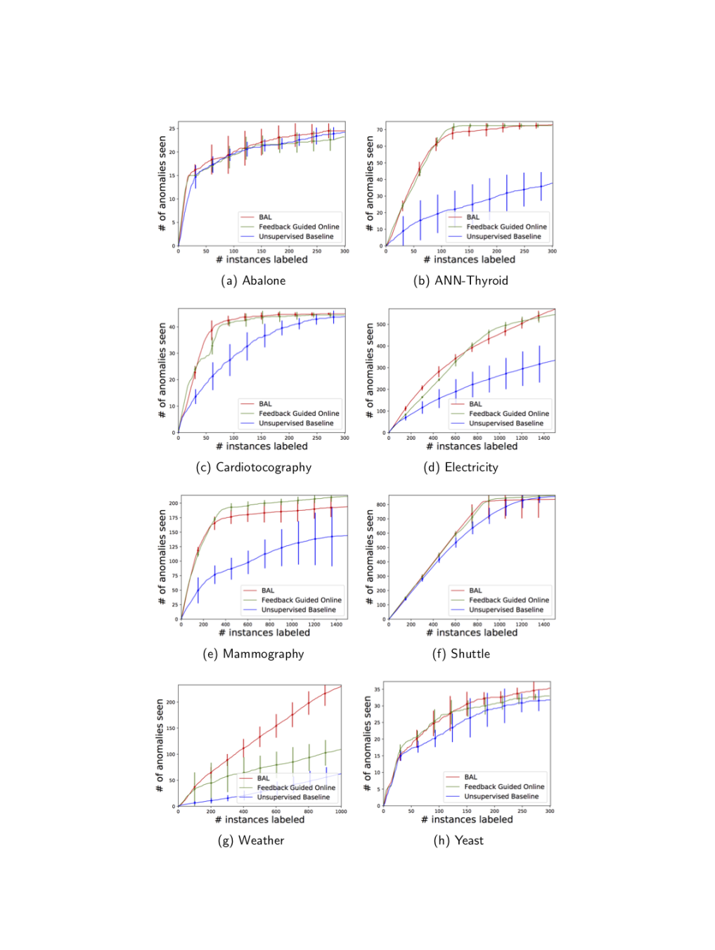
(a)

Figure 23: Results comparing BAL with feedback-guided anomaly detection via online optimization (?). BAL is the tree-based model implemented in our codebase and employs the AAD loss (anomalies score higher than $\tau$-th quantile score and nominals lower). Feedback Guided Online employs the linear loss in Siddiqui et al., 2018. Unsupervised Baseline is the unsupervised Isolation Forest baseline. Both approaches perform similar on most datasets. While BAL has slightly poor accuracy on Mammography than Feedback Guided Online, BAL performs much better on Weather.

Appendix C. Comparison of rule sets generated by Compact Descriptions and Bayesian Rulesets

Figure 24 compares the rule sets generated with Compact Descriptions and Bayesian Rulesets for the datasets not shown in Figure 18.

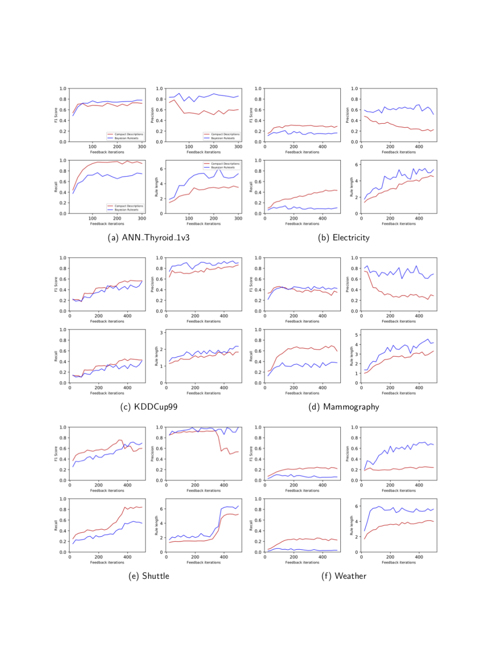
(a)

Figure 24: Results comparing BAL with feedback-guided anomaly detection via online optimization (?). BAL is the tree-based model implemented in our codebase and employs the AAD loss (anomalies score higher than $\tau$-th quantile score and nominals lower). Feedback Guided Online employs the linear loss in Siddiqui et al., 2018. Unsupervised Baseline is the unsupervised Isolation Forest baseline. Both approaches perform similar on most datasets. While BAL has slightly poor accuracy on Mammography than Feedback Guided Online, BAL performs much better on Weather.

References

- Abe et al. Abe, N., Zadrozny, B., & Langford, J. (2006). Outlier detection by active learning. In Proceedings of the Twelth ACM SIGKDD International Conference on Knowledge Discovery and Data Mining (KDD), pp. 504–509.
- Aggarwal Aggarwal, C. C. (2013). Outlier ensembles: position paper. ACM SIGKDD Explorations Newsletter, 14(2), 49–58.
- Aggarwal & Sathe Aggarwal, C. C., & Sathe, S. (2017). Outlier Ensembles - An Introduction. Springer.
- Almgren & Jonsson Almgren, M., & Jonsson, E. (2004). Using active learning in intrusion detection. In 17th IEEE Computer Security Foundations Workshop, (CSFW), p. 88.
- Balcan et al. Balcan, M., Broder, A. Z., & Zhang, T. (2007). Margin based active learning. In Proceedings of 20th Annual Conference on Learning Theory (COLT), pp. 35–50.
- Balcan & Feldman Balcan, M., & Feldman, V. (2015). Statistical active learning algorithms for noise tolerance and differential privacy. Algorithmica, 72(1), 282–315.
- Breunig et al. Breunig, M. M., Kriegel, H., Ng, R. T., & Sander, J. (2000). LOF: identifying density-based local outliers. In Proceedings of the 2000 ACM International Conference on Management of Data (SIGMOD), pp. 93–104.
- Chandola et al. Chandola, V., Banerjee, A., & Kumar, V. (2009). Anomaly detection: A survey. ACM computing surveys (CSUR), 41(3), 15:1–15:58.
- Chiang & Yeh Chiang, A., & Yeh, Y. (2015). Anomaly detection ensembles: In defense of the average. In IEEE/WIC/ACM International Conference on Web Intelligence and Intelligent Agent Technology, Volume III, pp. 207–210.
- Cohn et al. Cohn, D. A., Atlas, L. E., & Ladner, R. E. (1994). Improving generalization with active learning. Machine Learning, 15(2), 201–221.
- Das et al. Das, S., Wong, W., Dietterich, T. G., Fern, A., & Emmott, A. (2016). Incorporating expert feedback into active anomaly discovery. In IEEE 16th International Conference on Data Mining (ICDM), pp. 853–858.
- Das et al. Das, S., Wong, W.-K., Fern, A., Dietterich, T. G., & Siddiqui, M. A. (2017). Incorporating expert feedback into tree-based anomaly detection. In ACM SIGKDD International Conference on Knowledge Discovery & Data Mining (KDD), IDEA Workshop.
- Dasgupta et al. Dasgupta, S., Kalai, A. T., & Monteleoni, C. (2009). Analysis of perceptron-based active learning. Journal of Machine Learning Research (JMLR), 10, 281–299.
- Dheeru & Karra Taniskidou Dheeru, D., & Karra Taniskidou, E. (2017). UCI machine learning repository..
- Ditzler & Polikar Ditzler, G., & Polikar, R. (2013). Incremental learning of concept drift from streaming imbalanced data. IEEE Transactions on Knowledge and Data Engineering (TKDE), 25, 2283–2301.
- Domingues et al. Domingues, R., Filippone, M., Michiardi, P., & Zouaoui, J. (2018). A comparative evaluation of outlier detection algorithms: Experiments and analyses. Pattern Recognition, 74, 406–421.
- Doshi-Velez & Kim Doshi-Velez, F., & Kim, B. (2017). Towards a rigorous science of interpretable machine learning. arXiv:1702.08608.
- Emmott et al. Emmott, A., Das, S., Dietterich, T. G., Fern, A., & Wong, W. (2015). Systematic construction of anomaly detection benchmarks from real data. CoRR, abs/1503.01158.
- Freund et al. Freund, Y., Seung, H. S., Shamir, E., & Tishby, N. (1997). Selective sampling using the query by committee algorithm. Machine learning, 28(2-3), 133–168.
- Fürnkranz et al. Fürnkranz, J., Gamberger, D., & Lavrac, N. (2012). Foundations of Rule Learning. Cognitive Technologies. Springer.
- Goh & Rudin Goh, S. T., & Rudin, C. (2014). Box drawings for learning with imbalanced data. In The 20th ACM SIGKDD International Conference on Knowledge Discovery and Data Mining, (KDD), pp. 333–342.
- Görnitz et al. Görnitz, N., Kloft, M., Rieck, K., & Brefeld, U. (2013). Toward supervised anomaly detection. Journal of Artificial Intelligence Research (JAIR), 46, 235–262.
- Guha et al. Guha, S., Mishra, N., Roy, G., & Schrijvers, O. (2016). Robust random cut forest based anomaly detection on streams. In Proceedings of the 33nd International Conference on Machine Learning, (ICML), pp. 2712–2721.
- Harries & of New South Wales. Harries, M., & of New South Wales., U. (1999). Splice-2 comparative evaluation [electronic resource] : electricity pricing. University of New South Wales, School of Computer Science and Engineering [Sydney].
- He & Carbonell He, J., & Carbonell, J. G. (2007). Nearest-neighbor-based active learning for rare category detection. In Advances in Neural Information Processing Systems (NeurIPS), pp. 633–640.
- Jiménez Jiménez, D. (1998). Dynamically weighted ensemble neural networks for classification. In Proceedings of IEEE International Joint Conference on Neural Networks (IJNN), Vol. 1, pp. 753–756.
- Kalai et al. Kalai, A. T., Klivans, A. R., Mansour, Y., & Servedio, R. A. (2008). Agnostically learning halfspaces. SIAM Journal on Computing, 37(6), 1777–1805.
- Kearns Kearns, M. J. (1998). Efficient noise-tolerant learning from statistical queries. Journal of the ACM (JACM), 45(6), 983–1006.
- Lazarevic & Kumar Lazarevic, A., & Kumar, V. (2005). Feature bagging for outlier detection. In Proceedings of the Eleventh ACM SIGKDD International Conference on Knowledge Discovery and Data Mining (KDD), pp. 157–166.
- Letham et al. Letham, B., Rudin, C., McCormick, T. H., & Madigan, D. (2015). Interpretable classifiers using rules and bayesian analysis: Building a better stroke prediction model..
- Liu et al. Liu, F. T., Ting, K. M., & Zhou, Z. (2008). Isolation forest. In Proceedings of the IEEE International Conference on Data Mining (ICDM), pp. 413–422.
- Macha & Akoglu Macha, M., & Akoglu, L. (2018). Explaining anomalies in groups with characterizing subspace rules. Data Mining and Knowledge Discovery, 32(5), 1444–1480.
- Monteleoni Monteleoni, C. (2006). Efficient algorithms for general active learning. In Proceedings of 19th International Conference on Learning Theory (COLT), pp. 650–652.
- Nissim et al. Nissim, N., Cohen, A., Moskovitch, R., Shabtai, A., Edry, M., Bar-Ad, O., & Elovici, Y. (2014). ALPD: active learning framework for enhancing the detection of malicious PDF files. In Proceedings of IEEE Joint Intelligence and Security Informatics Conference (JISIC), pp. 91–98.
- Pevný Pevný, T. (2016). LODA: Lightweight online detector of anomalies. Machine Learning, 102(2), 275–304.
- Quinlan Quinlan, J. R. (1987). Generating production rules from decision trees. In Proceedings of the 10th International Joint Conference on Artificial Intelligence(IJCAI), pp. 304–307.
- Ribeiro et al. Ribeiro, M. T., Singh, S., & Guestrin, C. (2016). “why should I trust you?”: Explaining the predictions of any classifier. In Proceedings of the 22nd ACM SIGKDD International Conference on Knowledge Discovery and Data Mining (KDD), pp. 1135–1144.
- Ribeiro et al. Ribeiro, M. T., Singh, S., & Guestrin, C. (2018). Anchors: High-precision model-agnostic explanations. In Proceedings of the Thirty-Second AAAI Conference on Artificial Intelligence (AAAI-18), pp. 1527–1535.
- Settles Settles, B. (2012). Active Learning. Synthesis Lectures on Artificial Intelligence and Machine Learning. Morgan & Claypool Publishers.
- Siddiqui et al. Siddiqui, M. A., Fern, A., Dietterich, T. G., Wright, R., Theriault, A., & Archer, D. W. (2018). Feedback-guided anomaly discovery via online optimization. In Proceedings of the 24th ACM SIGKDD International Conference on Knowledge Discovery & Data Mining, (KDD), pp. 2200–2209.
- Stokes et al. Stokes, J. W., Platt, J. C., Kravis, J., & Shilman, M. (2008). ALADIN: Active learning of anomalies to detect intrusions. Technique Report, Microsoft Network Security Redmond, WA, 98052.
- Tan et al. Tan, S. C., Ting, K. M., & Liu, F. T. (2011). Fast anomaly detection for streaming data. In Proceedings of the 22nd International Joint Conference on Artificial Intelligence (IJCAI), pp. 1511–1516.
- Ted et al. Ted, E., Goldberg, H. G., Memory, A., Young, W. T., Rees, B., Pierce, R., Huang, D., Reardon, M., Bader, D. A., Chow, E., et al. (2013). Detecting insider threats in a real corporate database of computer usage activity. In Proceedings of the 19th ACM SIGKDD International Conference on Knowledge Discovery and Data Mining (KDD), pp. 1393–1401.
- Veeramachaneni et al. Veeramachaneni, K., Arnaldo, I., Korrapati, V., Bassias, C., & Li, K. (2016). : Training a big data machine to defend. Second IEEE International Conference on Big Data Security on Cloud, 49–54.
- Wang et al. Wang, T., Rudin, C., Doshi-Velez, F., Liu, Y., Klampfl, E., & MacNeille, P. (2016). Bayesian rule sets for interpretable classification. Proceedings of 16th IEEE International Conference on Data Mining (ICDM), 1269–1274.
- Woods et al. Woods, K. S., Doss, C. C., Bowyer, K. W., Solka, J. L., Priebe, C. E., & Kegelmeyer, W. P. (1993). Comparative evaluation of pattern recognition techniques for detection of microcalcifications in mammography. International Journal of Pattern Recognition and Artificial Intelligence, 07(06), 1417–1436.
- Wu et al. Wu, K., Zhang, K., Fan, W., Edwards, A., & Yu, P. S. (2014). Rs-forest: A rapid density estimator for streaming anomaly detection. In Proceedings of IEEE International Conference on Data Mining (ICDM), pp. 600–609.
- Yan & Zhang Yan, S., & Zhang, C. (2017). Revisiting perceptron: Efficient and label-optimal learning of halfspaces. In Advances in Neural Information Processing Systems (NeurIPS), pp. 1056–1066.
- Zimek et al. Zimek, A., Campello, R. J. G. B., & Sander, J. (2013). Ensembles for unsupervised outlier detection: challenges and research questions a position paper. SIGKDD Explorations, 15(1), 11–22.