The Three-Legged Tree Tensor Networks with $SU(2)$- and molecular point group symmetry

Abstract

We extend the three-legged tree tensor network state (T3NS) [J. Chem. Theory Comput. 2018, 14, 2026-2033] by including spin and the real abelian point group symmetries. T3NS intersperses physical tensors with branching tensors. Physical tensors have one physical index and at most two virtual indices. Branching tensors have up to three virtual indices and no physical index. In this way, T3NS combines the low computational cost of matrix product states and their simplicity for implementing symmetries, with the better entanglement representation of tree tensor networks. By including spin and point group symmetries, more accurate calculations can be obtained with lower computational effort. We illustrate this by presenting calculations on the bis($\mu$-oxo) and $\mu-\eta^{2}:\eta^{2}$ peroxo isomers of $[\mathrm{Cu}_{2}\mathrm{O}_{2}]^{2+}$. The used implementation is available on github.

Ghent University] Center for Molecular Modeling, Ghent University, Technologiepark 46, 9052 Zwijnaarde, Belgium [Ghent University] Department of Physics and Astronomy, Ghent University, Krijgslaan 281, S9, B-9000 Ghent, Belgium Ghent University] Department of Physics and Astronomy, Ghent University, Krijgslaan 281, S9, B-9000 Ghent, Belgium [University of Vienna] Vienna Center for Quantum Technology, University of Vienna, Boltzmanngasse 5, 1090 Vienna, Austria Ghent University] Center for Molecular Modeling, Ghent University, Technologiepark 46, 9052 Zwijnaarde, Belgium

1 Introduction

The discovery of the density matrix renormalization group (DMRG) by S. White in 1992^{1, 2} introduced a new and very successful way of treating strongly correlated quantum systems in both condensed matter physics and theoretical chemistry³. Later on, it was discovered that the DMRG wave function corresponds to a variational ansatz over the set of matrix product states (MPS)^{4, 5}. An MPS is a state that can be represented by a linear chain of tensors. It is the most simple form of a tensor network. The linear form of the MPS explained the high efficiency of DMRG for systems respecting the area law for entanglement in one-dimensional quantum spin systems.

In condensed matter physics, this kick-started the formulation of other (non-linear) tensor networks suitable for systems with another entanglement structure than the one-dimensional area law. The projected entangled pair states (PEPS)⁶ and the multiscale entanglement renormalization ansatz (MERA)⁷ are some notable examples.

The linear nature of the MPS is also far from ideal for the entanglement structure of most molecules. Hence, other tensor networks have also been studied in quantum chemistry, like the complete-graph tensor network states (CGTNS)⁸, the self-adaptive tensor network states (SATNS)⁹ and general tree tensor network states (TTNS)^{10, 11, 12}. However, due to its favorable computational complexity and the ease for exploitation of symmetries, the MPS is still the tensor network method of choice for quantum chemistry.

Recently, we introduced the Three-Legged Tree Tensor Network (T3NS)¹³, a subclass of the TTNS which allows an efficient optimization of the wave function while still enjoying the better entanglement representation of the TTNS. The tree-shaped network allows a logarithmic growing maximal distance with system size as apposed to the linear maximal distance for MPS.^{13, 10, 11, 14, 15, 16} In this paper, we will further extend the study of the T3NS. The implementation of symmetries will be explained and its advantages will be discussed theoretically as well as illustrated by exemplary calculations. More particularly, we will use the real abelian point group symmetries ($C_{1}$, $C_{i}$, $C_{2}$, $C_{s}$, $D_{2}$, $C_{2v}$, $C_{2h}$ and $D_{2h}$) and the $SU(2)$-symmetry present in the non relativistic quantum chemical Hamiltonian to obtain more accurate and faster calculations. We impose these global symmetries on the T3NS by using the Wigner-Eckart theorem as introduced by McCulloch for the MPS^{17, 18}.

The paper is structured as follows. In section 2, Three-legged Tree Tensor Networks and the advantages of this subset of the general tree tensor network are discussed. In section 3, the handling of symmetries in T3NS is illustrated. We incorporate the parity symmetry $\mathbb{Z}_{2}$, the number conservation $U(1)$, the spin symmetry $SU(2)$ and the real abelian molecular point group symmetries. We heavily rely on graphical depictions for the needed tensor contractions, as it yields a concise and clear notation for otherwise lengthy equations. In section 4, we show some calculations of T3NS with the previously mentioned symmetries. We compare results obtained for $[\mathrm{Cu}_{2}\mathrm{O}_{2}]^{2+}$with the ones presented in the original T3NS paper¹³. Summary and conclusions are provided in section 5.

The used implementation is open source and can be found on Github under the GNU GPLv3 license¹⁹.

2 Three-Legged Tree Tensor Networks

Figure 1: An example of a T3NS ansatz with 44 orbitals. Filled circles represent physical tensors which have one physical bond (not drawn here for simplicity) and maximally two virtual bonds. Unfilled circles represent branching tensors which have three virtual bonds and no physical bonds.

While the MPS ansatz of DMRG can be represented by a linear chain of tensors, the TTNS ansatz is built by making a tree-shaped network of tensors, making it the most general loop-less tensor network state.

The structure of the TTNS ansatz looks more faithful in the representation of the entanglement structure of molecules than the linear nature of the MPS ansatz. However, due to the branching of the network, the complexity for optimization becomes quickly unfeasible, especially for two-site optimization. Nakatani and Chan¹² introduced the half-renormalization for TTNS to allow efficient two-site optimizations. During the half-renormalization step the local optimization problem is exactly mapped to an MPS, which is then optimized. Although this mapping reduces the complexity per sweep, it also increases the number of sweeps needed for convergence.

The Three-Legged Tree Tensor Network¹³ is a subset of the general TTNS and an other method for circumventing the high complexity of the TTNS while still maintaining the advantages. In a T3NS, we make use of branching and physical tensors for the wave function ansatz and we intersperse these in the network. Physical tensors are the same as the tensors appearing in an MPS: they have one physical bond and maximally two virtual bonds. Branching tensors have three virtual bonds and no physical bonds. They allow the tensor network to branch. In a T3NS ansatz, branching tensors are never placed next to each other, since this would worsen the complexity for two-site optimization. Similarities exist between the T3NS ansatz and the half-renormalization of Nakatani and Chan¹². The mapping of the TTNS to an MPS corresponds with a branching tensor. The branching tensor is never explicitly optimized in the half-renormalization algorithm which results in the increased number of sweeps needed for convergence. For one-site optimization, half-renormalization is equivalent with a T3NS sweep where the branching tensors are never explicitly optimized. For two-site optimizations, the translation of half-renormalization to the T3NS is less straight forward but possible by reshaping the tensor network at each optimization step. We also note that a T3NS ansatz with only physical tensors corresponds with an MPS.

Another very important motivation for the restriction to tensors with three legs is the simplification of the implementation of $SU(2)$-symmetry. This is the main focus of this paper and will be discussed in the next section.

The resource requirements of the T3NS algorithm are presented in table 1. The scaling is explained in appendix A. An example of a T3NS wave function ansatz is given in fig. 1.

	DMRG	T3NS
CPU time:	$\mathcal{O}\left(k^{4}D^{2}+\underline{k^{3}D^{3}}\right)$	$\mathcal{O}\left(k^{4}D^{2}+\underline{k^{3}D^{4}}\right)$
Memory:	$\mathcal{O}\left(k^{3}D^{2}\right)$	$\mathcal{O}\left(k^{3}D^{2}+kD^{3}\right)$

Table 1: Resource requirements for DMRG and T3NS for quantum chemistry with renormalized operators. The underlined terms correspond with the complexity of the most intensive part of the algorithm, i.e. the matrix-vector product used in the iterative solver. The number of orbitals (or physical tensors in the network) is denoted by $k$ and the maximal virtual bond dimension is denoted by $D$.

3 Symmetries in T3NS

When representing the wave function in a tensor network ansatz, the encoding of symmetries into the network can facilitate the calculations. Depending on the particular tensor network ansatz used, the implementation of symmetries can be relatively straightforward or more involved. ^{18, 17, 20, 21, 22, 23, 24, 25, 26, 27} The usage of symmetries in the T3NS is facilitated by restricting to a maximum of three legs for every tensor in the wave function ansatz. This makes the treatment of both abelian and non-abelian global symmetries very analogous to the MPS, where this is already well studied^{18, 17, 20, 21, 22, 26, 27}.

3.1 Labeling the basis states

In the T3NS the index of a virtual (or physical) leg, specifies the different virtual (or physical) basis states traveling through this leg. The three-legged tensors are, due to the Wigner-Eckart theorem, irreducible tensor operators of the total symmetry group. The basis states need to transform according to the rows of the irreducible representations of the symmetry group.^{18, 17, 20, 21, 22} Each basis state $|\alpha\rangle$ (or index of a leg) can thus be labeled with the irrep and the row of the irrep according to which it transforms, i.e. $|\alpha\rangle=|\text{Irreps and rows},\alpha^{\prime}\rangle.$

The label $\alpha^{\prime}$ is needed to discern the different basis states belonging to the same list of irreps and rows of irreps. For a physical bond in non-relativistic quantum chemistry for example we need the local basis states at every orbital. We get

$$|-\rangle =|\pi=0,N_{\uparrow}=0,N_{\downarrow}=0\rangle$$ (1)

$$|\uparrow\rangle =|\pi=1,N_{\uparrow}=1,N_{\downarrow}=0\rangle$$ (2)

$$|\downarrow\rangle =|\pi=1,N_{\uparrow}=0,N_{\downarrow}=1\rangle$$ (3)

$$|\uparrow\downarrow\rangle =|\pi=0,N_{\uparrow}=1,N_{\downarrow}=1\rangle$$ (4)

for the parity $$\mathbb{Z}_{2} (\pi) U(1) (N_{\uparrow},N_{\downarrow})$$ , and two -symmetries for both the spin up and down , or

$$|-\rangle =|\pi=0,I=I_{0},N=0,j=0,m=0\rangle$$ (5)

$$|\uparrow\rangle =|\pi=1,I=I_{k},N=1,j=\frac{1}{2},m=\frac{1}{2}\rangle$$ (6)

$$|\downarrow\rangle =|\pi=1,I=I_{k},N=1,j=\frac{1}{2},m=-\frac{1}{2}\rangle$$ (7)

$$|\uparrow\downarrow\rangle =|\pi=0,I=I_{0},N=2,j=0,m=0\rangle$$ (8)

for $\mathbb{Z}_{2}$ $(\pi)$, $U(1)$ $(N)$, $SU(2)$ $(j,m)$ and the real abelian point-group symmetries $(I)$. The labels $\pi,N_{\uparrow},N_{\downarrow},N,j$ and $I$ represent irreps of the different symmetries, while $m$ labels the row of irrep $j$. $I_{k}$ is the point-group irrep of the orbital. A double occupation results in the trivial point group irrep $I_{0}$ since $I_{k}\otimes I_{k}=I_{0}$ for real abelian point group symmetries. In this example, $SU(2)$ is the only symmetry that needs an extra label for the row since the other symmetries have one-dimensional representations.

We omitted the label $\alpha^{\prime}$, since the irreps and rows already uniquely label the local physical basis states. However for the labeling of the virtual basis states the label $\alpha^{\prime}$ is still needed.

For calculations with fermions we utilize fermionic tensor networks. For every performed permutation or contraction the fermionic signs are calculated by looking at the parities of the different basis states.^{28, 13} One could note that labeling the parity $\pi$ is redundant since is it already fixed by the total number of particles in the state. However, we chose to keep explicitly track of the parity of the states. In this way, we can separate completely the fermionic sign handling from the particle numbers in the basis states. This allows a more modular implementation of the different symmetries and the fermionic signs.

3.2 Reduced tensors

$$\mathbf{A} =\sum_{\begin{smallmatrix}\pi_{1}I_{1}N_{1}j_{1}m_{1}\alpha_{1}\\ \pi_{2}I_{2}N_{2}j_{2}m_{2}\alpha_{2}\\ \pi_{3}I_{3}N_{3}j_{3}m_{3}\alpha_{3}\end{smallmatrix}}A_{\begin{smallmatrix}\pi_{1}I_{1}N_{1}j_{1}m_{1}\alpha_{1}\\ \pi_{2}I_{2}N_{2}j_{2}m_{2}\alpha_{2}\\ \pi_{3}I_{3}N_{3}j_{3}m_{3}\alpha_{3}\end{smallmatrix}}|\pi_{1}I_{1}N_{1}j_{1}m_{1}\alpha_{1}\rangle|\pi_{2}I_{2}N_{2}j_{2}m_{2}\alpha_{2}\rangle\langle\pi_{3}I_{3}N_{3}j_{3}m_{3}\alpha_{3}|$$ (9)

$$=\sum_{\mathbf{x}_{1}\alpha_{1}\mathbf{x}_{2}\alpha_{2}\mathbf{x}_{3}\alpha_{3}}\delta_{I_{1}\otimes I_{2},I_{3}}\delta_{\pi_{1}+\pi_{2}\bmod 2,\pi_{3}}\delta_{N_{1}+N_{2},N_{3}}\langle j_{1}m_{1}j_{2}m_{2}|j_{3}m_{3}\rangle\tilde{T}_{x_{1}\alpha_{1}x_{2}\alpha_{2}x_{3}\alpha_{3}}|\mathbf{x}_{1}\alpha_{1}\rangle|\mathbf{x}_{2}\alpha_{2}\rangle\langle\mathbf{x}_{3}\alpha_{3}|$$ (10)

$$=\sum_{\mathbf{x}_{1}\alpha_{1}\mathbf{x}_{2}\alpha_{2}\mathbf{x}_{3}\alpha_{3}}\delta_{\pi}\delta_{I}\delta_{N}\begin{pmatrix}j_{1}&j_{2}&j_{3}\\ m_{1}&m_{2}&-m_{3}\end{pmatrix}[j_{3}](-1)^{j_{3}-m_{3}}T_{x_{1}\alpha_{1}x_{2}\alpha_{2}x_{3}\alpha_{3}}|\mathbf{x}_{1}\alpha_{1}\rangle|\mathbf{x}_{2}\alpha_{2}\rangle\langle\mathbf{x}_{3}\alpha_{3}|.$$ (11)

$$\langle j_{1}m_{1}j_{2}m_{2}|j_{3}m_{3}\rangle=\begin{pmatrix}j_{1}&j_{2}&j_{3}\\ m_{1}&m_{2}&-m_{3}\end{pmatrix}\sqrt{2j_{3}+1}(-1)^{j_{1}-j_{2}+m_{3}}.$$ (12)

By using the labeling discussed in section 3.1, we can write every three-legged tensor in the wave function ansatz as shown in eq. 9. Due to the Wigner-Eckart theorem, the reducible tensor $A$ can be rewritten as a reduced tensor $\tilde{T}$ multiplied with the Clebsch-Gordan coefficients of the different symmetries as shown in eq. 10. These coefficients are Kronecker deltas for the real abelian symmetries and are the well-known Clebsch-Gordan coefficients for the recoupling of spins for $SU(2)$.

In eq. 11 the latter is replaced by the Wigner-3j symbol using eq. 12. Furthermore, several shorthand notations are introduced. $\mathbf{x}_{i}$ is shorthand notation for the full labeling of irreps and rows of irreps, while $x_{i}$ is the labeling of only the irreps and not the rows ($m$) of the basis state.

Shorthand notations are also introduced for the Kronecker deltas and for the square root of the multiplicity of $j_{i}$ $([j_{i}]=\sqrt{2j_{i}+1}$). A phase is absorbed in the reduced tensor $T$ (hence the transition from $\tilde{T}$ to $T$). We found the calculations particularly simple with this absorbed phase.

Eq. 11 expresses the reducible tensor $A$ in terms of a reduced tensor $T$ independent of the labels of the rows of irreps in $\mathbf{x}_{i}$ and a symmetry tensor. This symmetry tensor consists of the remaining terms in eq. 11. It contains the complete dependency of $A$ on the rows of irreps and is completely independent of the labels $\alpha_{i}$.

To construct the wave function, the different tensors in the network should be contracted. The physical tensors at the border of the network have one dangling uncontracted virtual bond since we assume that all physical tensors have two virtual bonds. For all but one bordering sites, this virtual bond of reduced dimension 1 will correspond with a ket state in eq. 10 with the same quantum numbers as the vacuum state. For the remaining bordering site, the dangling virtual bond of reduced dimension 1 will correspond with a bra state in eq. 10 with the same quantum numbers as the target state. By changing the allowed quantum numbers in this bond, we can easily change the quantum numbers of the targeted state. This is equivalent with the singlet-embedding strategy introduced by Sharma and Chan for spin-adapted DMRG²⁷.

Since the symmetry tensors targets all equivalent states in a multiplet at once, the complete wave function should be normalized by dividing by $[j_{\text{final}}]$, with $j_{\text{final}}$ the total spin quantum number of the target state.

The original network of reducible tensors representing the wave function (e.g. as given in fig. 1) now factorizes into two networks with the same shape. One network consists of reduced tensors. It covers the complete dependency of the labels $\alpha_{i}$ and is also dependent of the labeling of irreps. The other network is built from symmetry tensors. The dependency of the wave function on the labeling of the rows of irreps ($m$) is completely captured by this network. Furthermore, this network is completely independent of the labels $\alpha_{i}$.

3.2.1 Graphical depiction

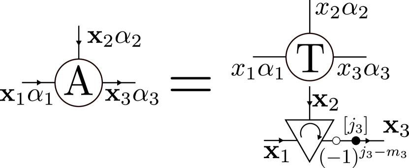
Figure 2: The ansatz for a three-legged tensor with symmetries. This is a graphical depiction of eq. 11. The reduced tensor and the symmetry tensor are represented by the upper and lower part, respectively.

In fig. 2 we introduce a graphical depiction of eq. 11. The triangle represents the Wigner-3j symbol and the various Kronecker deltas. The hollow circle represents $(-1)^{j_{3}-m_{3}}$ while the full circle represents $[j_{3}]$.

The direction of the arrows on the legs fixes the sign of $m_{i}$ in the Wigner sign. An incoming arrow corresponds with $m_{i}$, while an outgoing arrow is $-m_{i}$. Such a convention is also needed for a correct treatment of the fermionic signs.^{13, 28} An incoming leg for $\mathbf{x}_{i}$ represents $|\mathbf{x}_{i}\rangle$ while an outgoing leg represents $\langle\mathbf{x}_{i}|$.

The arrow in the triangle is needed to fix the order of the bra and kets in eq. 11. The arrow runs from the first bra or ket to the last bra or ket. Since the tensor is not invariant under permutation of these bras and kets, due to its fermionic character, the fixing of the order in our graphical depiction is needed. The arrow also represents the cyclic invariance of the Wigner-3j symbol. A phase has to be included for the Wigner symbol when changing the direction of the arrow but not when rotating the arrow. A quick summary of the graphical depiction is also given in appendix B.1.

3.2.2 Sparsity and compression of the tensors

The symmetry tensor encodes a lot of sparsity since it consists out of several Kronecker deltas and a Wigner-3j symbol which respects the triangle inequality. In this way, it is easy to see which elements of the reduced tensor $T$ do not contribute to the resulting reducible tensor $A$. Such index combinations can be omitted from the optimization.

Next to sparsity, the symmetry tensor also compresses the data. This is clear since both the symmetry tensors and the reduced tensors need to be summed over $x_{i}$ (or $\pi_{i}I_{i}N_{i}j_{i}$) when contracting, while only the symmetry tensor need to be summed over $m_{i}$ for a contraction. This last summation is completely independent of the tensor $T$, simplifying the calculations.

3.3 The Chemical Hamiltonian

The non-relativistic quantum chemical Hamiltonian is given by

$$H=\sum_{ij}t_{ij}\sum_{\sigma}c^{\dagger}_{i\sigma}c_{j\sigma}+\frac{1}{2}\sum_{ijkl}V_{ijkl}\sum_{\sigma\tau}c^{\dagger}_{i\sigma}c^{\dagger}_{j\tau}c_{l\tau}c_{k\sigma},$$ (13)

where $i,j,k$ and $l$ are indices for the different spatial orbitals and $\sigma,\tau$ represent the spin degree of freedom $(\uparrow$ or $\downarrow)$.

For the four point interactions this separates into the following cases:

$$V_{iikk} c^{\dagger}_{i\uparrow}c^{\dagger}_{i\downarrow}c_{k\downarrow}c_{k\uparrow}, i=j,k=l$$ (14)

$$V_{iikl} \left(c^{\dagger}_{i\uparrow}c^{\dagger}_{i\downarrow}c_{l\downarrow}c_{k\uparrow}+c^{\dagger}_{i\uparrow}c^{\dagger}_{i\downarrow}c_{k\downarrow}c_{l\uparrow}\right), i=j,k<l$$ (15)

$$V_{ijkk} \left(c^{\dagger}_{i\uparrow}c^{\dagger}_{j\downarrow}c_{k\downarrow}c_{k\uparrow}+c^{\dagger}_{j\uparrow}c^{\dagger}_{i\downarrow}c_{k\downarrow}c_{k\uparrow}\right), i<j,k=l$$ (16)

$$V_{ijkl} (c^{\dagger}_{i\uparrow}c^{\dagger}_{j\uparrow}c_{l\uparrow}c_{k\uparrow}+c^{\dagger}_{i\uparrow}c^{\dagger}_{j\downarrow}c_{l\downarrow}c_{k\uparrow}+$$

$$\ c^{\dagger}_{i\downarrow}c^{\dagger}_{j\uparrow}c_{l\uparrow}c_{k\downarrow}+c^{\dagger}_{i\downarrow}c^{\dagger}_{j\downarrow}c_{l\downarrow}c_{k\downarrow}) i<j,k<l$$

$$+ \left(k\leftrightarrow l\right),$$ (17)

where we only used $V_{ijkl}=V_{jilk}$. The complete Hamiltonian can be constructed by summing these terms for all possible $(i,j,k,l)$-combinations.

The creation and annihilation operators $c^{\dagger}_{k\sigma}$ and $c_{k\sigma}$ do not yet transform according to the rows of the $SU(2)$-irreps. As is well known²², an additional phase has to be introduced. One possible transformation is given by

$$\tilde{c}^{\dagger}_{k\sigma} =c^{\dagger}_{k\sigma}$$ (18)

$$\tilde{c}_{k\sigma} =(-1)^{\frac{1}{2}+\sigma}c_{k-\sigma}.$$ (19)

In this way, we can again split off the Clebsch-Gordan coefficients into a symmetry tensor.

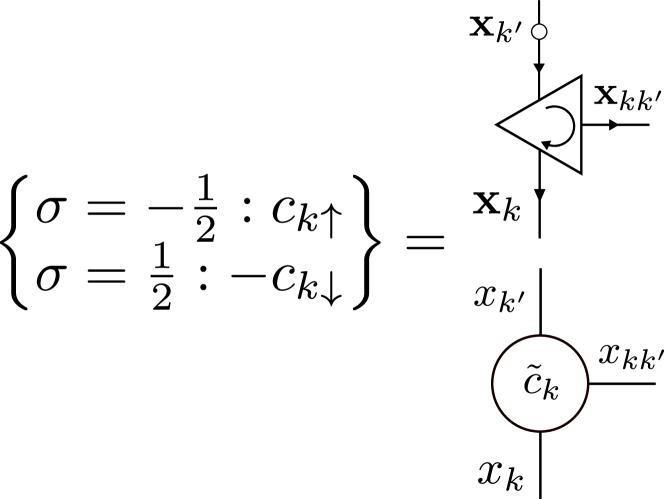
Figure 3: Graphical depiction of the annihilation operator on site $k$. The operators are represented by a symmetry tensor and a reduced tensor. $\mathbf{x}_{k}$ and $\mathbf{x}_{k^{\prime}}$ are the local basis states for orbital $k$. The third index $\mathbf{x}_{kk^{\prime}}=\left(1,I_{k},-1,\frac{1}{2},\sigma\right)$ serves the purpose of correctly coupling different operators. No bonds here need an extra $\alpha$ label, as stated in section 3.1.

The decomposition of the annihilation operators into a reduced tensor and a symmetry tensor is graphically depicted in fig. 3. One can easily calculate the tensor elements for the reduced tensors in fig. 3. For the creation operators the graphical depiction is completely equivalent.

The most illustrative example is given by eq. 17 since here four different spatial orbitals can be involved. The construction of these terms is graphically shown in fig. 4 where

$$F_{J}=-[J]\left(V_{ijkl}+(-1)^{J}V_{ijlk}\right).$$ (20)

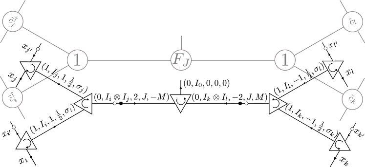
Figure 4: Graphical depiction of the terms in eq. 17. The upper gray layer are the reduced tensors and the lower layer are the symmetry tensors. Labels of connected bonds are written fully for clarity. The different operators need to couple to the trivial singlet, since the term in eq. 17 transforms trivially under the used symmetries.

The tensor network in fig. 4 should be manipulated to the same geometry of the tensor network of the wave function. For obtaining a T3NS structure out of fig. 4, two types of transformations are needed. First, the order of the operators (e.g. switching $i$ and $k$) can be changed by using properties of the Wigner symbols and taking an appropriate fermionic sign into account. One can also insert identities into the network in fig. 4. These two transformations suffice to change the network in fig. 4 to an arbitrary T3NS network.

All terms in eq. 14, 15, 16 and 17 can be manipulated in this way. The most important point here is that both the wave function ansatz and the Hamiltonian are represented by the same tensor network shape and both are factorized into a reduced tensor network and a symmetry tensor network.

3.4 The optimization

In the previous sections 3.2 and 3.3, we have shown that both the wave function ansatz and the Hamiltonian can be factorized into a reduced tensor network and a symmetry tensor network. In this section, we briefly discuss how this representation can be used during the optimization algorithm of the T3NS.

The optimization of a T3NS occurs in a similar way as for DMRG, i.e. we sweep through the network and optimize only two tensors at a time. During this local optimization of the network, the effect of the Hamiltonian on the other tensors (i.e. the environment) can be efficiently captured by renormalized operators.^{3, 29, 22, 30} The usage of renormalized operators reduces the quartic scaling of the total chemical Hamiltonian as a function of the number of orbitals to a quadratic scaling for the effective Hamiltonian.

These renormalized operators are partial contractions of the Hamiltonian and the T3NS wave function. More specifically, the energy of a wave function $E~{}=~{}\langle\Psi|H|\Psi\rangle$ can be calculated by sandwiching the Hamiltonian terms in their network form between the wave function and its adjoint in the same network form. This triple-layered network of reduced and symmetry tensors can be fully contracted to obtain the energy. However, during the optimization of only two sites of the network, a lot of the triple-layered network can be precontracted and reused since it does not change during this optimization step. The renormalized operators are exactly these precontracted parts of the network. A graphical depiction of a renormalized operator is given in fig. 5. This is an object which has indices $\mathbf{x}_{1}$, $\mathbf{x}_{1^{\prime}}$ and $\mathbf{x}_{11^{\prime}}$. These indices are explained in the caption of fig. 5.

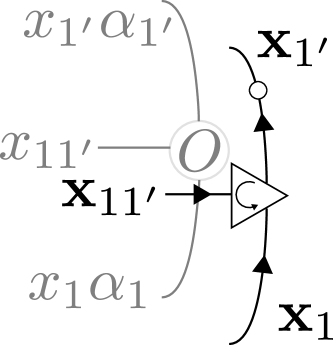
Figure 5: Graphical depiction of a renormalized operator. Both the symmetry tensor and the reduced tensor $O$ are shown. The index $\mathbf{x}_{1}$ ($\mathbf{x}_{1^{\prime}}$) originates from the T3NS ansatz of the ket (bra) wave function. The index $\mathbf{x}_{11^{\prime}}$ corresponds with a bond of the network representation of the Hamiltonian. The tensor $O$ is the resulting reduced tensor from partial contraction of the triple-layered network.

After the optimization of the two sites, the sweep algorithm moves on to a neighboring pair of two sites, which has one site in common with the previous pair. These sites are optimized by a new effective Hamiltonian. In order to calculate this effective Hamiltonian through renormalized operators, one can recycle certain of these operators and update others. This is in fact equivalent with the usage of renormalized operators in DMRG for quantum chemistry.

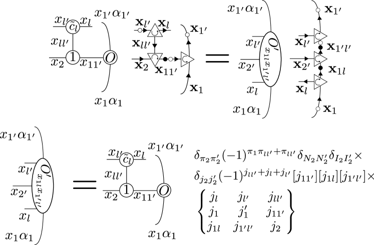
Figure 6: The appending of a site-operator $\tilde{c}_{l}$ to a renormalized operator is shown. The symmetry tensors change of form to ease following calculations in the algorithm. The reduced tensors are contracted and the result is permuted appropriately. Only index $1$ and $1^{\prime}$ need an extra $\alpha$-label to discern between the different basis states.

In fig. 6, an example of such an update is given. A site operator (as given in fig. 3) is appended to an already existing renormalized operator. The resulting tensor is then manipulated to another form, for an easier construction of the effective Hamiltonian. In the example, the manipulation of the symmetry tensors gives rise to extra factors. A Wigner-9j symbol arises due to the recoupling of the spin basis states. The phase $(-1)^{\pi_{1}\pi_{ll^{\prime}}+\pi_{ll^{\prime}}}$ originates from the fermionic character of the tensors.

Wigner symbols are used for the update of renormalized operators and the construction of the effective Hamiltonian when a branching tensor is optimized. However, when only physical tensors are optimized, no Wigner symbols are needed. This is discussed in more depth in appendix B.3. The optimization of two adjacent physical tensors is exactly the same as in DMRG.

As a side remark, the present implementation, omitting branching tensors, can perform a DMRG algorithm which only needs Wigner symbols during the update of renormalized operators and not during the iterative optimization step.

More details for the construction of the effective Hamiltonian and the updating of the renormalized operators are given in appendix B.

4 Calculations

In this section, we present several calculations with T3NS. The used implementation for the calculations can be found on github¹⁹. This implementation is able to exploit $\mathbb{Z}_{2}$, $U(1)$, $SU(2)$ and the real abelian point group symmetries. The symmetries can be included in a modular way. This enables us to compare calculations with and without $SU(2)$ and point group symmetries for the same implementation.

After the optimization of two sites, this two-site object has to be split into two separate sites again. This is done by the Singular Value Decomposition (SVD). The truncation of the virtual bond dimension during this step is done in two different ways.

First, a fixed maximal bond dimension can be imposed. The algorithm will keep as many singular values into consideration as possible. It will first select the largest singular values until no non-zero singular values are left or the maximal bond dimension is reached. The remaining singular values and their corresponding basis states are discarded.

Second, the dynamic block state selection (DBSS) can be used^{31, 32}. With this method, the algorithm keeps the largest singular values until a threshold for a cost function is reached. The cost function used in our implementation is given by

$$w_{disc}=\sum_{i_{disc}}s_{i_{disc}}^{2}$$ (21)

i.e. the sum of the squares of all discarded singular values. This corresponds with $\langle\Psi_{disc}|\Psi_{disc}\rangle$, with $|\Psi_{disc}\rangle$ the discarded part of the wave function during truncation. Other cost functions can be easily implemented.

Next to a targeted threshold, a minimal and maximal bond dimension should be specified. Throwing away too many basis states at a certain stage can impede the optimization at later stages, even though the truncation error is only minimal at that point. Specifying a minimal bond dimension ensures a certain flexibility at all time. The maximal bond dimension is needed to prevent a large increase in both run time and memory usage when the imposed threshold can not be reached.

As noted in section 3.2.2, the usage of symmetries with irreps that are more than one-dimensional, such as $SU(2)$, introduces a compression of the wave function. Different basis states belonging to the same multiplet can be represented by a singular reduced basis state. Analogous to the bond dimension being the number of basis states kept in the bond, the reduced bond dimension is defined as the number of reduced basis states kept. When using $SU(2)$, the reduced bond dimension of the bonds, and not the bond dimension, will reflect the computational complexity.

Just as with DMRG for quantum chemistry, keeping track of the renormalized operators is the most taxing part on memory for T3NS. The amount of renormalized operators needing to be stored for T3NS are of the same order as for DMRG. However, T3NS calculations can be performed on a considerably lower bond dimension for a similar accuracy. Consequently, this lowers the storage requirements for the renormalized operators and allows us to keep all tensors on memory at all time. No checkpoint files need to be written to disk or read from disk during the algorithm for the present system sizes and bond dimensions.

4.1 The Bisoxo and Peroxo Isomer of $[\mathrm{Cu}_{2}\mathrm{O}_{2}]^{2+}$

We revisit the bis($\mu$-oxo) and the $\mu=\eta^{2}:\eta^{2}$ peroxo $[\mathrm{Cu}_{2}\mathrm{O}_{2}]^{2+}$isomers as a test case for T3NS with $SU(2)$ and abelian point group symmetries. These transition-metal clusters have been previously studied by other ab initio methods such as the complete active space self-consistent field theory (CASSCF), the complete active space self-consistent field theory with second order perturbation theory (CASPT2),³³ the restricted active space self-consistent field theory with second order perturbation theory (RASPT2)³⁴, DMRG^{31, 35} and DMRG+CT³⁶ (DMRG with canonical transformation theory). It was the largest system studied in the initial T3NS paper using only $U(1)\otimes U(1)$ symmetry¹³ (i.e. conservation of both particle number and spin projection).

We perform calculations for both isomers in an (26e, 44o) active space. The same active space is used as in refs. 13, 31. Both isomers have a $D_{2h}$ point group symmetry and their ground state is a singlet state in the $A_{g}$ irrep of $D_{2h}$.³¹ When using the $SU(2)$ and/or point group symmetry adapted version of T3NS, states corresponding to these irreps will be targeted. The same T3NS shape and orbital ordering is used as in ref. 13. We also perform calculations of the lowest lying triplet state in the $A_{g}$ irrep of $D_{2h}$ for both isomers.

4.1.1 The Bisoxo isomer with and without spin symmetry

In order to compare the present spin adapted version of T3NS with its non-adapted predecessor¹³, we perform several calculations for the bisoxo isomer at different bond dimensions and with different symmetries included.

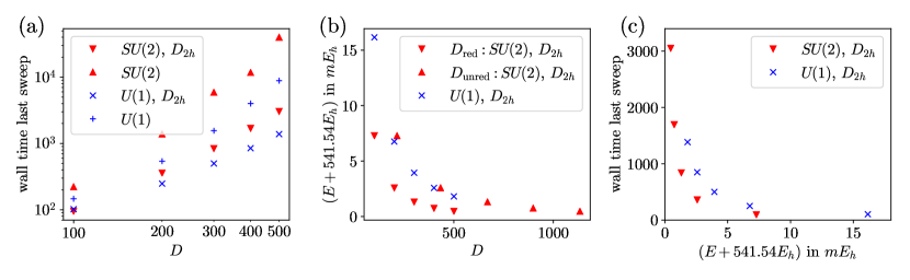
Figure 7: Results for the bisoxo isomer obtained on an 18-core Intel Xeon Gold 6140 (Skylake at 2.3 GHz). Calculations with a fixed maximal bond dimension of $D=100,200,300,400$ and $500$ were performed. Results for $U(1)\otimes U(1)$ combined with or without $D_{2h}$ are given by crosses. Results for $U(1)\otimes SU(2)$ combined with or without $D_{2h}$ are given by triangles. The bond dimensions are in this case the reduced bond dimensions, except for (b) where also unreduced bond dimensions are shown. (a) shows the wall time of the last sweep for different bond dimensions and different symmetries. (b) shows the ground state energy for different bond dimensions. For the spin-adapted calculations, both the maximal reduced as unreduced bond dimensions are given. (c) shows wall time of last sweep in function of ground state energy.

In fig. 7(a), timings for the last sweep are shown for several fixed bond dimensions. Calculations were performed with $U(1)\otimes U(1)$ symmetry and with $SU(2)\otimes U(1)$ symmetry. For both, calculations with and without the $D_{2h}$ point group symmetry are done. For the spin-adapted versions, the bond dimensions shown are the reduced bond dimensions.

As expected, the usage of the point group symmetry introduces a lot of sparsity in the tensors which speeds up calculations considerably. Calculation time improved by a factor of 6 and 13 at $D=500$ for $U(1)\otimes U(1)$ and $SU(2)\otimes U(1)$ respectively when including $D_{2h}$. For both calculations with or without spin symmetry, the inclusion of $D_{2h}$ yields practically the same energies and maximal truncation errors as when performing the calculation without the point group symmetry.

For tensors of the same size, calculations including spin symmetry are computationally more intensive than without spin symmetry as can be seen in fig. 7(a). This is expected since the reduced tensors are more dense than the reducible tensors. However, the compressed nature of the reduced tensors (see section 3.2.2) makes spin-adapted calculations at a certain reduced bond dimension more accurate than calculations without spin symmetry at an equal bond dimension. This can be seen in figure 7(b). The maximal unreduced bond dimension during $SU(2)$ calculations is also given in this figure. For the present calculations, the maximal unreduced bond dimension is approximately twice as large as the imposed maximal reduced bond dimension. When comparing wall time with achieved accuracy, the calculations with $SU(2)$ included are considerably faster, as is shown in fig. 7(c).

4.1.2 The bisoxo and peroxo isomers with spin symmetry

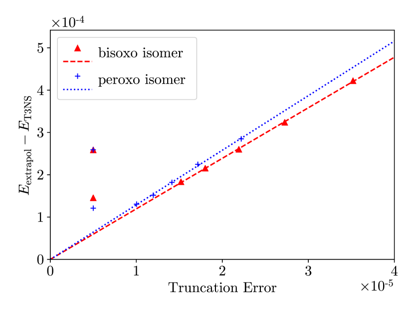
Figure 8: Extrapolation of the energy for both the bisoxo and peroxo isomer. Extrapolation is done by using the results for $D=600,700,800,900$ and $1000$. The DBSS calculations of table 2 targeting a truncation error of $5\cdot 10^{-6}$ are also shown in the figure. They are however not used for the extrapolation.

Method	$E_{\mathrm{bisoxo}}[\mathrm{E_{h}}]$	$E_{\mathrm{peroxo}}[\mathrm{E_{h}}]$	$\Delta E$ [kcal/mol]
DMRG31	-541.53853	-541.58114	26.7
T3NS with $U(1)\otimes U(1)$13
500	-541.53820	-541.58094	26.8
T3NS with $U(1)\otimes SU(2)\otimes D_{2h}$
300	-541.53869	-541.58119	26.7
500	-541.53954	-541.58171	26.5
$500,5\cdot 10^{-6}$	-541.53986	-541.58183	26.3
1000	-541.53993	-541.58197	26.4
$1000,5\cdot 10^{-6}$	-541.53997	-541.58198	26.4
Extrapolated	-541.54012	-541.58210	26.3

Table 2: Energy gaps and ground state energies between the bisoxo and peroxo isomers. The energy gaps are given in kcal/mol. Ground state energies are given in Hartree. For T3NS calculations with fixed bond dimension, the bond dimension is given in the first column. For T3NS calculations using DBSS, the minimal bond dimension and the truncation error is given. For T3NS with $SU(2)$ the given bond dimensions are the reduced ones. Maximum bond dimensions around 2000 were reported for both clusters during the DMRG calculations of ref. 31.

Several calculations are performed for both isomers. Both $SU(2)$ and $D_{2h}$ symmetry are used. The inclusion of spin and point group symmetry considerably improves our calculations and allows us to go to much larger bond dimensions. Both a constant maximal bond dimension and DBSS are used. Some obtained results are shown in table 2 alongside previously published results. Calculations at a fixed reduced bond dimension of 300 already surpassed the most accurate DMRG calculations of ref. 31 and the most accurate T3NS calculations of ref. 13. For the most accurate calculation the maximal reduced bond dimension needed were 1626 and 1329 for the bisoxo and peroxo isomer respectively.

A linear extrapolation^{37, 29} between the truncation error and the energy is performed. The extrapolation is based on results with a fixed maximal reduced bond dimension of $D=600,700,800,900$ and $1000$. This extrapolation is shown in fig. 8. The results for the DBSS calculations in table 2 are also given in the figure. For both systems, two DBSS calculations are performed, both targeting a truncation error of $5\cdot 10^{-6}$. They use however another minimal bond dimension. Although the same truncation error is targeted for both DBSS calculations, the accuracy of the two calculations is quite different due to their different minimal bond dimensions. Because of this, only the calculations with fixed bond dimension are used for the extrapolation. A linear extrapolation looks justified for these calculations. The extrapolated values are given in table 2.

The lowest lying triplet states in the $A_{g}$ irrep are also calculated for both isomers. These states are easily targeted by changing the allowed quantum numbers in the outgoing target state of the T3NS (as discussed in section 3.2) and are similar in computation time as for the singlet states. We obtained an energy of $E=-541.46194E_{h}$ and $E=-541.40184E_{h}$ for the bisoxo and peroxo isomer respectively when a maximal reduced bond dimension of 1000 was chosen.

5 Conclusion

In this paper we extended the T3NS ansatz with $SU(2)$ and real abelian point group symmetries. This ansatz combines the computational efficiency of DMRG and its ease of implementing symmetries with the rich entanglement representation of the TTNS. We show that implementing spin and real abelian point group symmetries is not much more involved than for DMRG.^{18, 17, 20, 21, 22}

Several calculations for the bisoxo and peroxo isomers of $[\mathrm{Cu}_{2}\mathrm{O}_{2}]^{2+}$are presented. Calculations are performed both with and without spin and point group symmetries. They illustrate the substantial advantages of using the $SU(2)$ and point group symmetries of the chemical Hamiltonian. For a given accuracy, the computational time decreases with every included symmetry.

For these calculations, the same, rather intuitive, orbital ordering as in the preliminary T3NS-paper is used¹³. Advanced techniques for the ordering of orbitals, like the usage of entanglement measures,³¹ and its effect on the accuracy will be of interest in subsequent research. Furthermore, results can be improved through the development of post-T3NS methods, in similarity to post-DMRG methods. Some notable examples of post-DMRG methods which can readily be adapted are DMRG-SCF,^{38, 39, 40} DMRG-CASPT2 ^{41, 42} and DMRG-TCCSD (DMRG-tailored coupled cluster with single and double excitations)^{43, 44}.

From an intuitive point of view, the T3NS ansatz looks a more natural representation of the entanglement structure of molecules than the linear MPS. We expect that the T3NS will, in general, be able to provide a more compact and accurate parametrization of the wave function. If this also results in more efficient computations is at this moment not clear yet. However, in our preliminary paper¹³, we noted that, for the few tested systems, T3NS needed an increasingly smaller bond dimension compared to the MPS with increasing system size. This supports the idea that with large enough system sizes the T3NS will become the tensor network of choice. To assess this trend, we need to study larger system sizes. The entanglement structure and efficiency for both the MPS and T3NS for larger system sizes will be one of the main focus points in subsequent research.

K.G. acknowledges support from the Research Foundation Flanders (FWO Vlaanderen). Computational resources (Stevin Supercomputer Infrastructure) and services were provided by Ghent University. We gratefully acknowledge fruitful discussions with Örs Legeza and Sebastian Wouters.

Appendix A Computational complexity

Two differences can be noted between the computational complexity given in the original T3NS-paper¹³ and the one given in this paper.

First, no disk resource requirements are given here, since our current implementation does not store intermediate results on disk. All tensors are kept in memory at all time.

Second, the CPU time of the T3NS has been lowered from $\mathcal{O}(k^{5}D^{2}+k^{3}D^{4})$ to $\mathcal{O}(k^{4}D^{2}+k^{3}D^{4})$. In the previous paper, we stated the complexity for updating renormalized operators with branching tensors to be $\mathcal{O}(k^{5}D^{2})$ for quantum chemistry. It was noted that the recombination of two single operators in both sets of renormalized operators to a complimentary double operator was the most intensive part. The worst case scenario for this is indeed $\mathcal{O}(k^{4}D^{2})$ and since there are $\mathcal{O}(k)$ branching tensors in the network where this can occur, we previously obtained $\mathcal{O}(k^{5}D^{2})$. However not all branching tensors will result in this worst case scaling of $\mathcal{O}(k^{4}D^{2})$, and only the most central ones in the network will have this scaling. A more rigorous analysis showed an overall upper bound of $\mathcal{O}(k^{4}D^{2})$ instead.

Appendix B Working with symmetry tensors

In this appendix we explain the T3NS with fermionic reduced tensors and their symmetry tensors in more depth. We begin with a short summary of the graphical notations used (Appendix B.1). In Appendix B.2, we use the gauge freedom of the tensor network to define a canonical form of the tensors, in correspondence with the canonical form in DMRG. In appendix B.3, we give a few examples of contractions of renormalized operators with two-site tensors. In appendix B.4, some cases for updating the renormalized operators are given.

B.1 Shorthand and graphical notation

We introduced a graphical depiction for the symmetry and reduced tensors used in the T3NS algorithm in section 3.2.1. We shortly summarize the different used notations in table 3. It is useful to notice the effect of changing the direction of an arrow on the Clebsch Gordan coefficients of the symmetries.

$\mathbf{x}_{i}$	$\pi_{i}I_{i}N_{i}j_{i}m_{i}\alpha_{i}$
$x_{i}$	$\pi_{i}I_{i}N_{i}j_{i}\alpha_{i}$
	$\begin{array}[]{c}\delta_{I_{1}\otimes I_{2},I_{3}}\delta_{\pi_{1}+\pi_{2}\bmod 2,\pi_{3}}\delta_{N_{1}+N_{2},N_{3}}\\ \begin{pmatrix}j_{1}&j_{2}&j_{3}\\ m_{1}&m_{2}&-m_{3}\end{pmatrix}|\mathbf{x}_{1}\rangle|\mathbf{x}_{2}\rangle\langle\mathbf{x}_{3}|\end{array}$
	$\begin{array}[]{c}\delta_{I_{2}\otimes I_{3},I_{1}}\delta_{\pi_{2}+\pi_{3}\bmod 2,\pi_{1}}\delta_{N_{2}+N_{3},N_{1}}\\ \begin{pmatrix}j_{1}&j_{2}&j_{3}\\ m_{1}&-m_{2}&-m_{3}\end{pmatrix}|\mathbf{x}_{1}\rangle\langle\mathbf{x}_{2}|\langle\mathbf{x}_{3}|\end{array}$
	$\sqrt{2j_{i}+1}$
	$(-1)^{j_{i}-m_{i}}$

Table 3: Used graphical depictions and shorthand notations.

B.2 The canonical form

The representation of a wave function by a tensor network is not unique. To show this gauge freedom, we contract the tensor $A[x]$ with an invertible matrix $Y$ and the neighboring tensor $A[x+1]$ with $Y^{-1}$^{22, 45}:

$$\tilde{A}[x]_{ijk^{\prime}} =\sum_{k}A[x]_{ijk}Y_{kk^{\prime}}$$ (22)

$$\tilde{A}[x+1]_{k^{\prime}lm} =\sum_{k}(Y^{-1})_{k^{\prime}k}A[x+1]_{klm}.$$ (23)

When contracting these two new tensors $\tilde{A}[x]$ and $\tilde{A}[x+1]$, we obtain the exact result as contracting the original tensors. This freedom is present at every virtual bond in the tensor network.

Although one can use the gauge freedom in general tensor networks to define a canonical form,^{45, 46, 47} it is more straightforward in loopfree finite tensor networks. In this canonical form one tensor is chosen as orthogonality center. The currently optimized tensor is normally chosen for this. Other tensors are orthogonal with respect to contraction over all bonds but the one leading to the orthogonality center. Calculating the overlap of the tensor network with itself now simplifies to a complete contraction of the orthogonality center with its adjoint since the contributions of the other tensors simplify to unit tensors. This allows us to optimize the orthogonality center through an ordinary eigenvalue problem instead of a general one.

All tensors of the T3NS wave function are of the form given in eq. 9. Depending on the indices that are contracted, tensors of this form can be orthogonal in different ways.

For such a reducible tensor which is orthogonal to a contraction over index 1 and 2 we propose that the reduced tensor should be orthogonal as well with respect to a contraction over index 1 and 2. Furthermore, the adjoint of the reduced tensor (i.e. the corresponding reduced tensor for the bra wave function) is given by its hermitian.

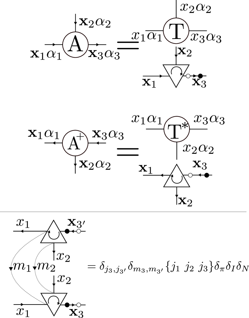
Figure 9: Upper: an orthogonalized tensor with respect to contraction over leg 1 and 2 and its adjoint. Lower: contracting the two symmetry tensors by summation over $m$ simplifies the contraction. $\{j_{1}\ j_{2}\ j_{3}\}$ represents the triangle inequality.

A graphical depiction for this case is given in fig. 9. In the bottom of fig. 9 it is shown how the symmetry tensors simplify the contraction. Indeed, with help of the symmetry tensors and the orthogonality of $T$, one can show that

$$\mathcal{C}(\mathbf{A}\mathbf{A}^{+})=\sum_{\mathbf{x}_{3}\alpha_{3}}|\mathbf{x}_{3}\alpha_{3}\rangle\langle\mathbf{x}_{3}\alpha_{3}|~{}.$$ (24)

If the same reducible tensor has to be orthogonal with respect to a contraction over index 2 and 3, the reduced tensor should be again orthogonal with respect to that contraction. We use the gauge freedom to move a factor of $\sqrt{2j_{1}+1}$ from a neighboring tensor to this tensor and a factor of $\sqrt{2j_{3}+1}$ from this tensor to a neighboring tensor (see the different position of the solid circle in fig. 9 and fig. 10).

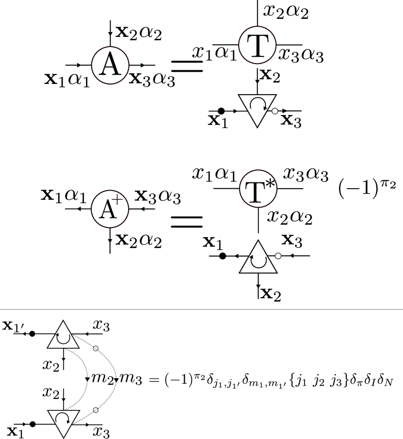
Figure 10: Upper: an orthogonalized tensor with respect to contraction over leg 2 and 3 and its adjoint. Lower: contracting the two symmetry tensors by summation over $m$ simplifies the contraction. $\{j_{1}\ j_{2}\ j_{3}\}$ represents the triangle inequality. The term $(-1)^{\pi_{2}}$ is introduced due to the fermionic nature of the tensors.

The adjoint of the reduced tensor is given again by its hermitian, but now, also an extra phase needs to be introduced. This can be seen in fig. 10. The phase is needed for imposing orthogonality due to the fermionic nature of the tensors. The introduction of this phase does not pose a problem as long the contraction over all adjoint tensors of the network results in the expected bra wave function. This can be ensured by correcting all the introduced phases in the adjoint of the orthogonality center. We get indeed for the orthogonalized tensor given in fig. 10 that

$$\mathcal{C}(\mathbf{A}\mathbf{A}^{+})=\sum_{\mathbf{x}_{1}\alpha_{1}}|\mathbf{x}_{1}\alpha_{1}\rangle\langle\mathbf{x}_{1}\alpha_{1}|~{}.$$ (25)

B.3 Optimizing tensors

The renormalized operators are used during the optimization of two contiguous sites. Depending on the nature of the two sites, a different kind of optimization is needed. If both sites are physical, a DMRG-like optimization step is used. Two sets of renormalized operators are used to calculate the effect of the effective Hamiltonian on the two-site object. This kind of optimization is shown in fig. 11(a). During this optimization step, no Wigner symbols are needed. It also means that, in this formulation, one can do an optimization of a DMRG-chain which only needs Wigner symbols when appending site-operators to the renormalized operators.

If one of the two sites is a branching site, a T3NS optimization step is needed. During this optimization, three sets of renormalized operators are used to calculate the effect of the effective Hamiltonian on the two site object. An example of this optimization step is shown in fig. 11(b). Depending on where the physical tensor is attached to the branching tensor, variants of fig. 11(b) are needed, giving rise to slightly different prefactors.

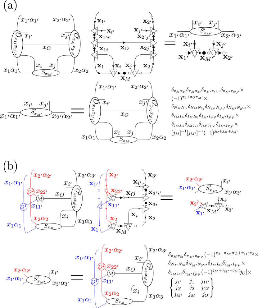
Figure 11: (a) The effect of the effective Hamiltonian on a two-site object consisting out of two physical sites. (b) The effective Hamiltonian on a two-site object consisting out of one physical and one branching site. Tensor $M$ is a tensor needed for the merging of the renormalized operators and its value can be found by deforming the network in fig. 4 to the same form as the T3NS network.

B.4 Updating renormalized operators

After every optimization step of the algorithm the renormalized operators need to be updated with the newly found optimized tensors. In section 3.4, we already discussed appending a site-operator to a renormalized operator (see fig. 6). Here, we show how a physical tensor or a branching tensor can be used to update the renormalized operators.

In fig. 12, a physical tensor is used to update a renormalized operator with a site-operator appended to it. The physical tensor used in this figure is orthogonal with respect to a contraction over leg 2 and 3 (see fig. 10).

In fig. 13, a branching tensor is used to recombine two renormalized operators to a new one. The branching tensor in this example is orthogonal with respect to a contraction over leg 1 and 2 (see fig. 9).

Similar graphical depictions can be made for both fig. 12 and 13 when using tensors orthogonalized in different ways. Both the appending of a site tensor and the recombination of two renormalized operators through usage of a branching tensor need Wigner-9j symbols. Updating of a renormalized operator through usage of a physical tensor does not need any Wigner symbols.

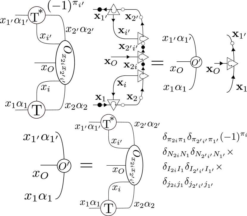
Figure 12: Update of a renormalized operator with a site-operator attached. This operator can be obtained as shown in fig. 6. The update is done by using a orthogonalized physical tensor and its adjoint. In this example, the tensor is orthogonalized with respect to contraction over bond i and 2.

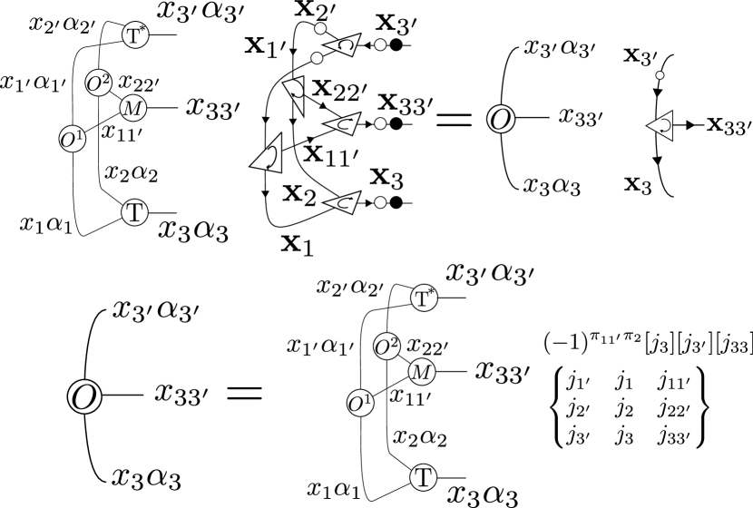
Figure 13: Recombination of two renormalized operators to a new one. The recombination is done by using an orthogonalized branching tensor and its adjoint. In this example, the tensor is orthogonalized with respect to contraction over bond 1 and 2. Tensor $M$ is a tensor needed for the merging of the two renormalized operators and its value can be found by deforming the network in fig. 4 to the same form as the T3NS network.

References

- White 1992 White, S. R. Density matrix formulation for quantum renormalization groups. Phys. Rev. Lett. 1992, 69, 2863–2866
- White 1993 White, S. R. Density-matrix algorithms for quantum renormalization groups. Phys. Rev. B 1993, 48, 10345–10356
- White and Martin 1999 White, S. R.; Martin, R. L. Ab initio quantum chemistry using the density matrix renormalization group. J. Chem. Phys. 1999, 110, 4127–4130
- Rommer and Östlund 1997 Rommer, S.; Östlund, S. Class of ansatz wave functions for one-dimensional spin systems and their relation to the density matrix renormalization group. Phys. Rev. B 1997, 55, 2164–2181
- Östlund and Rommer 1995 Östlund, S.; Rommer, S. Thermodynamic Limit of Density Matrix Renormalization. Phys. Rev. Lett. 1995, 75, 3537–3540
- Verstraete and Cirac 2004 Verstraete, F.; Cirac, J. I. Renormalization algorithms for Quantum-Many Body Systems in two and higher dimensions. eprint arXiv:cond-mat/0407066 2004,
- Vidal 2007 Vidal, G. Entanglement Renormalization. Phys. Rev. Lett. 2007, 99, 220405
- Marti et al. 2010 Marti, K. H.; Bauer, B.; Reiher, M.; Troyer, M.; Verstraete, F. Complete-graph tensor network states: a new fermionic wave function ansatz for molecules. New J. Phys. 2010, 12, 103008
- Kovyrshin and Reiher 2017 Kovyrshin, A.; Reiher, M. Self-adaptive tensor network states with multi-site correlators. J. Chem. Phys. 2017, 147, 214111
- Murg et al. 2015 Murg, V.; Verstraete, F.; Schneider, R.; Nagy, P.; Legeza, Ö. Tree tensor network state with variable tensor order: an efficient multireference method for strongly correlated systems. J. Chem. Theory Comput. 2015, 11, 1027–1036
- Murg et al. 2010 Murg, V.; Verstraete, F.; Legeza, Ö.; Noack, R. M. Simulating strongly correlated quantum systems with tree tensor networks. Phys. Rev. B 2010, 82, 205105
- Nakatani and Chan 2013 Nakatani, N.; Chan, G. K.-L. Efficient tree tensor network states (TTNS) for quantum chemistry: Generalizations of the density matrix renormalization group algorithm. J. Chem. Phys. 2013, 138, 134113–134113
- Gunst et al. 2018 Gunst, K.; Verstraete, F.; Wouters, S.; Legeza, Ö.; Van Neck, D. T3NS: Three-Legged Tree Tensor Network States. J. Chem. Theory Comput. 2018, 14, 2026–2033
- Wouters and Van Neck 2014 Wouters, S.; Van Neck, D. The density matrix renormalization group for ab initio quantum chemistry. Eur. Phys. J. D 2014, 68, 272
- Ferris 2013 Ferris, A. J. Area law and real-space renormalization. Phys. Rev. B 2013, 87, 125139
- Shi et al. 2006 Shi, Y.-Y.; Duan, L.-M.; Vidal, G. Classical simulation of quantum many-body systems with a tree tensor network. Phys. Rev. A 2006, 74, 022320
- McCulloch 2007 McCulloch, I. P. From density-matrix renormalization group to matrix product states. J. Stat. Mech.: Theory Exp. 2007, 2007, P10014–P10014
- McCulloch and Gulácsi 2002 McCulloch, I. P.; Gulácsi, M. The non-Abelian density matrix renormalization group algorithm. Europhys. Lett. 2002, 57, 852–858
- Gunst 2018 Gunst, K. T3NS: An implementation of the Three-Legged Tree Tensor Network algorithm. https://github.com/klgunst/T3NS, 2018
- Singh et al. 2010 Singh, S.; Pfeifer, R. N. C.; Vidal, G. Tensor network decompositions in the presence of a global symmetry. Phys. Rev. A 2010, 82, 050301
- Singh et al. 2010 Singh, S.; Zhou, H.-Q.; Vidal, G. Simulation of one-dimensional quantum systems with a global SU(2) symmetry. New J. Phys. 2010, 12, 033029
- Wouters et al. 2014 Wouters, S.; Poelmans, W.; Ayers, P. W.; Van Neck, D. CheMPS2: A free open-source spin-adapted implementation of the density matrix renormalization group for ab initio quantum chemistry. Comput. Phys. Commun. 2014, 185, 1501–1514
- Weichselbaum 2012 Weichselbaum, A. Non-abelian symmetries in tensor networks: A quantum symmetry space approach. Ann. Phys. 2012, 327, 2972–3047
- Singh and Vidal 2012 Singh, S.; Vidal, G. Tensor network states and algorithms in the presence of a global SU(2) symmetry. Phys. Rev. B 2012, 86, 195114
- Hubig 2018 Hubig, C. Abelian and non-abelian symmetries in infinite projected entangled pair states. SciPost Phys. 2018, 5, 47
- Tóth et al. 2008 Tóth, A. I.; Moca, C. P.; Legeza, Ö.; Zaránd, G. Density matrix numerical renormalization group for non-Abelian symmetries. Phys. Rev. B 2008, 78, 245109
- Sharma and Chan 2012 Sharma, S.; Chan, G. K.-L. A spin-adapted Density Matrix Renormalization Group algorithm for quantum chemistry. J. Chem. Phys. 2012, 136, 124121
- Bultinck et al. 2017 Bultinck, N.; Williamson, D. J.; Haegeman, J.; Verstraete, F. Fermionic matrix product states and one-dimensional topological phases. Phys. Rev. B 2017, 95, 075108
- Chan and Head-Gordon 2002 Chan, G. K.-L.; Head-Gordon, M. Highly correlated calculations with a polynomial cost algorithm: A study of the density matrix renormalization group. J. Chem. Phys. 2002, 116, 4462–4476
- Kurashige and Yanai 2009 Kurashige, Y.; Yanai, T. High-performance ab initio density matrix renormalization group method: Applicability to large-scale multireference problems for metal compounds. J. Chem. Phys. 2009, 130, 234114
- Barcza et al. 2011 Barcza, G.; Legeza, Ö.; Marti, K. H.; Reiher, M. Quantum-information analysis of electronic states of different molecular structures. Phys. Rev. A 2011, 83, 012508
- Szalay et al. 2015 Szalay, S.; Pfeffer, M.; Murg, V.; Barcza, G.; Verstraete, F.; Schneider, R.; Legeza, Ö. Tensor product methods and entanglement optimization for ab initio quantum chemistry. Int. J. Quantum Chem. 2015, 115, 1342–1391
- Cramer et al. 2006 Cramer, C. J.; Włoch, M.; Piecuch, P.; Puzzarini, C.; Gagliardi, L. Theoretical Models on the Cu2O2 Torture Track: Mechanistic Implications for Oxytyrosinase and Small-Molecule Analogues. J. Phys. Chem. A 2006, 110, 1991–2004
- Malmqvist et al. 2008 Malmqvist, P. Å.; Pierloot, K.; Shahi, A. R. M.; Cramer, C. J.; Gagliardi, L. The restricted active space followed by second-order perturbation theory method: Theory and application to the study of CuO2 and Cu2O2 systems. J. Chem. Phys. 2008, 128, 204109
- Phung et al. 2016 Phung, Q. M.; Wouters, S.; Pierloot, K. Cumulant Approximated Second-Order Perturbation Theory Based on the Density Matrix Renormalization Group for Transition Metal Complexes: A Benchmark Study. J. Chem. Theory Comput. 2016, 12, 4352–4361
- Yanai et al. 2010 Yanai, T.; Kurashige, Y.; Neuscamman, E.; Chan, G. K.-L. Multireference quantum chemistry through a joint density matrix renormalization group and canonical transformation theory. J. Chem. Phys. 2010, 132, 024105
- Legeza et al. 2003 Legeza, Ö.; Röder, J.; Hess, B. A. Controlling the accuracy of the density-matrix renormalization-group method: The dynamical block state selection approach. Phys. Rev. B 2003, 67, 125114
- Zgid and Nooijen 2008 Zgid, D.; Nooijen, M. The density matrix renormalization group self-consistent field method: Orbital optimization with the density matrix renormalization group method in the active space. J. Chem. Phys. 2008, 128, 144116
- Wouters et al. 2014 Wouters, S.; Bogaerts, T.; Van Der Voort, P.; Van Speybroeck, V.; Van Neck, D. Communication: DMRG-SCF study of the singlet, triplet, and quintet states of oxo-Mn(Salen). J. Chem. Phys. 2014, 140, 241103
- Ghosh et al. 2008 Ghosh, D.; Hachmann, J.; Yanai, T.; Chan, G. K.-L. Orbital optimization in the density matrix renormalization group, with applications to polyenes and -carotene. J. Chem. Phys. 2008, 128, 144117
- Kurashige and Yanai 2011 Kurashige, Y.; Yanai, T. Second-order perturbation theory with a density matrix renormalization group self-consistent field reference function: Theory and application to the study of chromium dimer. J. Chem. Phys. 2011, 135, 094104
- Wouters et al. 2016 Wouters, S.; Van Speybroeck, V.; Van Neck, D. DMRG-CASPT2 study of the longitudinal static second hyperpolarizability of all-trans polyenes. J. Chem. Phys. 2016, 145, 054120
- Veis et al. 2016 Veis, L.; Antalík, A.; Brabec, J.; Neese, F.; Legeza, Ö.; Pittner, J. Coupled Cluster Method with Single and Double Excitations Tailored by Matrix Product State Wave Functions. J. Phys. Chem. Lett. 2016, 7, 4072–4078
- Faulstich et al. 2018 Faulstich, F. M.; Máté, M.; Laestadius, A.; András Csirik, M.; Veis, L.; Antalik, A.; Brabec, J.; Schneider, R.; Pittner, J.; Kvaal, S.; Legeza, Ö. Numerical and Theoretical Aspects of the DMRG-TCC Method Exemplified by the Nitrogen Dimer. arXiv e-prints 2018, arXiv:1809.07732
- Evenbly 2018 Evenbly, G. Gauge fixing, canonical forms, and optimal truncations in tensor networks with closed loops. Phys. Rev. B 2018, 98, 085155
- Zaletel and Pollmann 2019 Zaletel, M. P.; Pollmann, F. Isometric Tensor Network States in Two Dimensions. eprint arXiv:1902.05100v1 2019,
- Haghshenas et al. 2019 Haghshenas, R.; O’Rourke, M. J.; Chan, G. K.-L. Canonicalization of projected entangled pair states. eprint arXiv:1903.03843v2 2019,