Fourth-order spin correlation function in the extended central spin model

Abstract

Spin noise spectroscopy has developed into a very powerful tool to access the electron spin dynamics. While the spin-noise power spectrum in an ensemble of quantum dots in a magnetic field is essentially understood, we argue that the investigation of the higher order cumulants promises to provide additional information not accessible by the conventional power noise spectrum. We present a quantum mechanical approach to the correlation function of the spin-noise power operators at two different frequencies for small spin bath sizes and compare the results with a simulation obtained from the classical spin dynamics for large number of nuclear spins. This bispectrum is defined as a two-dimensional frequency cut in the parameter space of the fourth-order spin correlation function. It reveals information on the influence of the nuclear-electric quadrupolar interactions on the long-time electron spin dynamics dominated by a magnetic field. For large bath sizes and spin lengths the quantum mechanical spectra converge to those of the classical simulations. The broadening of the bispectrum across the diagonal in the frequency space is a direct measure of the quadrupolar interaction strength. A narrowing is found with increasing magnetic field indicating a suppression of the influence of quadrupolar interactions in favor of the nuclear Zeeman effect.

I Introduction

Optical spin noise spectroscopy (SNS) Sinitsyn and Pershin (2016) has been established as a minimally invasive probe to study the electron spin dynamics and was originally proposed by Aleksandrov and Zapasskii Aleksandrov and Zapasskii (1981); Zapasskii (2013). Off-resonant Faraday rotation measurements were used for nearly perturbation-free measurement of the spin noise in an ensemble of alkali atoms Crooker et al. (2004), as well as in bulk semi-conductors Oestreich et al. (2005); Crooker et al. (2009); Berski et al. (2015). In the absence of an external magnetic field, SNS was able to reveal the influence of the electrical-nuclear quadrupolar interactions on an ensembles of semi-conductor quantum dots (QD) Hanson et al. (2007) onto the long-time decay Bechtold et al. (2015); Uhrig et al. (2014) of the second-order spin correlation function $C_{2}(t)=\langle S_{z}(t)S_{z}\rangle$ as well as on its spin-noise power spectrum Crooker et al. (2010); Li et al. (2012); Glasenapp et al. (2016); Hackmann and Anders (2014); Hackmann et al. (2015); Wu et al. (2016); Sinitsyn et al. (2012).

The information extracted from the second order correlation function, however, is limited to macroscopic linear effects by the fluctuation dissipation theorem, if only the thermal equilibrium is considered. For this reason many experimental studies utilized non-equilibrium conditions, generated by radio frequency Glasenapp et al. (2014); Poggio et al. (2009); Degen et al. (2007) or through periodic laser pulses Young et al. (2002); Jäschke et al. (2018); Greilich et al. (2006a, b); Jäschke et al. (2017); Varwig et al. (2016).

Applying an external magnetic field to a QD whose strength is exceeding the Overhauser field Merkulov et al. (2002); Testelin et al. (2009) generated by the surrounding fluctuating nuclear spins, however, suppresses the effect of these quadrupolar interactions onto $C_{2}(t)$ Glasenapp et al. (2016). Yet, quadrupolar interactions play an important role in the understanding of the long-time decay of higher-order spin response functions Press et al. (2010); Bechtold et al. (2016); Fröhling and Anders (2017) especially at large magnetic fields above 1T. Since those fourth-order spin correlation functions Press et al. (2010); Bechtold et al. (2016); Fröhling and Anders (2017) have been investigated in the time domain, it has been suggested Li et al. (2013); Li and Sinitsyn (2016) to extend the conventional SNS to higher-order spin noise correlations. The third-order spin correlation of the type $C_{3}(t_{1},t_{2},t_{3})=\langle S_{z}(t_{1})S_{z}(t_{2})S_{z}(t_{3})\rangle$ requires time-reversal symmetry breaking for non-zero values, is imaginary in the time domain in thermal equilibrium and is, therefore, not an observable.

In this paper, we focus on the spectral information of the fourth-order correlation functions Li and Sinitsyn (2016); Li et al. (2013); Fröhling and Anders (2017) in the weak measurement regime. While it has been established that the real-time fourth order spin correlation functions contain important information on the field-dependent long-time scale of the decay Press et al. (2010); Bechtold et al. (2016) that was connected to competition between the nuclear quadrupolar couplings and the Zeeman energy Fröhling and Anders (2017), not much is know on the spectral information of the fourth order correlation function Li and Sinitsyn (2016); Li et al. (2013).

In a recent publication Hägele et al. proposed an approach to higher-order cumulants and their spectra in the context of a continuous quantum noise measurement Hägele and Schefczik (2018). The authors used a time evolution of the density operator by combining the von Neumann equation with a Markovian damping through the environment and a feedback term generated by the continuous measurement of the property of interest. They applied their method to calculate the fourth-order correlation spectrum for two coupled spins in a finite magnetic field.

We present and compare two far simpler approaches based on the linear response theory that is tailored to the nearly perturbation free optical SNS Li and Sinitsyn (2016); Li et al. (2013); Crooker et al. (2010, 2009) and is easily applicable to a wide range of scenarios. We are interested in the correlations between the spin-noise power spectrum operator at two different frequencies. For independent noise variables and purely Gaussian noise, the correlation function would factorize and the cumulant Kubo (1962) would vanish. If the spin dynamics is coherent, this fourth-order spin correlation function yields only non-vanishing contributions at the same frequencies.

We focus on the spin dynamics in a semi-conductor quantum dot since it is considered as promising candidate for a quantum bit Bennett and DiVincenzo (2000); Burkard et al. (2000); Loss and DiVincenzo (1998). We analyze the influence of the spin length and number of nuclear spins onto the fourth-order spin noise spectra using the central spin model (CSM) Gaudin (1976) and its extension to nuclear electric quadrupolar couplings Sinitsyn et al. (2012); Hackmann et al. (2015) which is well suited to describe quantum dot systems Merkulov et al. (2002); Coish and Loss (2004); Al-Hassanieh et al. (2006); Glazov and Ivchenko (2012). We show that the spectra calculated by our quantum mechanical method approach the results obtained by a semiclassical simulation Chen et al. (2007); Jäschke et al. (2017) in the limit of larger spins and bath sizes. In the opposite limit, we are able to reproduce the higher-order spin spectra in the case of two coupled spins in a finite magnetic field presented in Ref. Hägele and Schefczik (2018).

The main obstacle for the realization of a quantum bit Bennett and DiVincenzo (2000); Burkard et al. (2000); Loss and DiVincenzo (1998) by a QD ensemble is the loss of information, as the electron spin decays over time due to its coupling to a fluctuating environment. While spin decoherence due to free electron motion is suppressed in a quantum dot, the high localization causes the hyperfine interaction between the electron spin and the surrounding nuclear spins to dominate. A detailed investigation of interaction processes influencing the spin dynamics in quantum dots on all time scale is desirable.

The standard SNS was successfully established as a very useful tool to obtain the basis information on the spin dynamics. However, spectral information on very weak interactions such as the nuclear quadrupolar interactions or the influence of the dipole-dipole interactions is lost rather quickly in a finite magnetic field larger than the Overhauser field. We propose to investigate the fourth-order spin noise spectrum since the shape of the cumulant spectra is significantly altered in the presence of the nuclear quadrupolar interactions even in larger external magnetic fields. Therefore, the fourth-order spin noise spectrum reveals additional information on the long time dynamics that is not accessible with the standard SNS. We are able to link the change in the spectroscopic data to the magnetic field dependency of the long-time decay time in higher-order correlations functions Bechtold et al. (2015); Press et al. (2010); Fröhling and Anders (2017).

A short introduction of the model and its semi-classical approximation in Sec. II is followed by the definition of the second and fourth-order cumulant of the electron spin in Sec. III. Quantum mechanical and classical implementation of the higher-order correlations are presented in Sec. IV. The results are discussed in Sec. V. The influence of the external magnetic field on the spin cumulant is investigated and the classical simulation is discussed as a limit to the quantum-mechanical approach. The quadrupolar interaction is included into the model. Classical and quantum mechanical treatment will provide an insight into its effect on the higher order spectrum. A brief summary is given in Sec. VI.

II Model

While an electron spin in a singly negatively charged QD is well isolated from decoherence due to fluctuating charge environments, the strong localisation of the electronic wave function increases the coupling between the electron spin and its surrounding nuclear spins. The spin dynamics in the QD is governed by interactions acting on vastly different time scales ranging from the hyperfine interaction ($\sim 1$ ns) Sinitsyn et al. (2012); Hackmann et al. (2015) to the dipole-dipole interaction ($\sim 100$ $\upmu$s) Merkulov et al. (2002). The quadrupolar interaction caused by electric strain fields and the nuclear spin depends highly on sample growth. We will confine ourselves to the dominating interactions for the spin dynamics in a quantum dot: The hyperfine interaction, the Zeeman interaction of the spins with the external magnetic field $\vec{B}_{\text{ext}}$, and the nuclear-electron quadrupolar interaction.

II.1 Central spin model

Both the hyperfine interaction as well as the Zeeman energy of the spins in an external magnetic field $\vec{B}_{\text{ext}}$ is described by the Hamiltonian of the central spin model Gaudin (1976):

$$\begin{split}\tilde{H}_{\text{CSM}}=g_{e}\mu_{B}\vec{B}_{\text{ext}}\vec{S}+\mu_{N}\vec{B}_{\text{ext}}\sum_{k=1}^{N}g_{N,k}\vec{I}_{k}+\sum_{k=1}^{N}\tilde{A}_{k}\vec{I}_{k}\vec{S}.\end{split}$$ (1)

$g_{e}$ denotes the g-factor of the electron, $g_{N,k}$ accounts for the g-factor of the $k$-th nucleus, and $\mu_{N}$ is the nuclear magneton. The third term represents the hyperfine interaction between the electronic central spin $\vec{S}$ and the bath comprised $N$ nuclear spins $\vec{I}_{k}$ conveyed by the coupling constants $\tilde{A}_{k}$. In negatively charged QDs the hyperfine interaction is isotropic Hackmann and Anders (2014). The fluctuation frequency

$$\omega^{2}_{\mathrm{fluc}}=\frac{4}{3}\langle\vec{I}^{2}\rangle\sum_{k=1}^{N}\tilde{A}_{k}^{2}$$ (2)

of the Overhauser field

$$\vec{B}_{N}=\sum_{k=1}^{N}\tilde{A}_{k}\vec{I}_{k}$$ (3)

is used to define the intrinsic time scale $T^{\ast}=1/\omega_{\mathrm{fluc}}$ which describes the short-time electron spin decoherence induced by the fluctuation of the Overhauser field. Typical values of 1-3 ns are found for $T^{\ast}$ in experiments, depending on their lateral size Hackmann et al. (2015); Bechtold et al. (2015). The expectation value of the nuclear spin length $\langle\vec{I}^{2}\rangle$ takes the value $I(I+1)$ in the quantum mechanical case while for the classical approximation, we obtain the spin length $\langle\vec{I}^{2}\rangle=I^{2}$.

(In,Ga)As/GaAs QDs contain different isotopes with different spin lengths. While Ga and As isotopes are characterized by a nuclear spin of $I_{Ga}=I_{As}=3/2$, In has a spin $I_{In}=9/2$. Therefore, the influence of different $I$ on higher order correlation functions will be discussed at length in this paper.

The time scale $T^{*}$ can be utilized to introduce a dimensionless Hamiltonian

$$H=T^{\ast}\tilde{H}_{\text{CSM}}$$ (4)

with the dimensionless hyperfine coupling constants $a_{k}=T^{\ast}\tilde{A}_{k}$ and the dimensionless external magnetic field $\vec{b}_{\mathrm{ext}}=T^{\ast}g_{e}\mu_{B}\vec{B}_{\text{ext}}$. Assuming that all nuclear spins have the same $g$-factor it is convenient to define

$$\zeta=\frac{g_{N}\mu_{N}}{g_{e}\mu_{B}},$$ (5)

the ratio between nuclear and electron Zeeman energy. Then, the Hamiltonian takes the dimensionless form

$$\begin{split}H_{\text{CSM}}=&\vec{S}\vec{b}_{\mathrm{ext}}+\zeta\vec{b}_{\mathrm{ext}}\sum_{k=1}^{N}\vec{I}_{k}+\sum_{k=1}^{N}a_{k}\vec{I}\vec{S}.\end{split}$$ (6)

The hyperfine coupling constants $\tilde{A}_{k}$ are proportional to the probability of the electron at the location of the $k$th nucleus, $\tilde{A}_{k}\propto|\psi_{e}(\vec{R}_{k})|^{2}$. We assume the envelope of the electron wave function in a $d$-dimensional quantum dot with the radius $L_{0}$ is of the form

$$\psi_{e}(\vec{r})=CL_{0}^{-{d}/2}\exp\left(-\frac{|\vec{r}|^{m}}{2L_{0}^{m}}\right),$$ (7)

with $m=1$ describing a hydrogen-like and $m=2$ a Gaussian envelope function. $C$ is a dimensionless normalization constant. With the coupling constant dependent on the probability of an electron being present at the position of the $k$th nucleus, $\tilde{A}_{k}\sim|\psi|^{2}$, the realization of hyperfine coupling constants thus becomes

$$\tilde{A}_{k}=A_{\text{max}}\exp\left(-\frac{|\vec{r}|^{m}}{L_{0}^{m}}\right).$$ (8)

Due to the growth strain in an semiconductor quantum dot the quadrupolar moment of the nucleus interacts with the strained electronic charge distribution in the QD. In case of axial symmetry regarding the local easy axis $\vec{n}_{k}$, the quadrupolar interaction is represented by the Hamiltonian Sinitsyn et al. (2012); Dzhioev and Korenev (2007); Bulutay (2012)

$$H_{Q}=\sum_{k}H_{q}^{k}=\sum_{k}q_{k}(\vec{I}_{k}\vec{n}_{k})^{2}.$$ (9)

The quadrupolar interaction constants $q_{k}$ are a measure of the quadrupolar interaction strength at the $k$th nucleus and are quantified by the second derivative of the electron strain field along the easy axis. The local easy axis $\vec{n}_{k}^{z}$ have been reported to be at a mean deviation angle of $\overline{\theta}=23^{\circ}$ with the growth axis Bulutay (2012) for an In_0.4Ga_0.6As QD.

II.2 Semi-classical approximation

In the semiclassical approximation, we replace the quantum mechanical spin operator with classical vectors and average over all possible initial spin configurations Chen et al. (2007); Merkulov et al. (2002); Stanek et al. (2014). In numerical simulations, the integral over all Bloch spheres are replaced by the discrete configuration sample that introduces some finite statistical error that is well controlled by the number of configurations.

The basis of the classical simulation is a set of coupled equations of motion for the central electronic spin $\vec{S}$ and the individual nuclear spins $\vec{I}_{k}$ Merkulov et al. (2002); Stanek et al. (2014). Those can be derived as the classical limit from the quantum mechanical Hamiltonian Eq. (6) via a path integral formalism Chen et al. (2007); Al-Hassanieh et al. (2006). By solving

$$\dfrac{\mathrm{d}\vec{S}}{\mathrm{d}t} =\left(\vec{b}_{\mathrm{ext}}+\sum_{k}a_{k}\vec{I}_{k}\right)\times\vec{S}=\vec{b}_{\mathrm{tot},S}\times\vec{S},$$ (10)

$$\dfrac{\mathrm{d}\vec{I}_{k}}{\mathrm{d}t} =\left(\zeta\vec{b}_{\mathrm{ext}}+a_{k}\vec{S}\right)\times\vec{I}_{k}=\vec{b}_{\mathrm{tot},I_{k}}\times\vec{I}_{k}$$ (11)

for different realizations of the initial spin state from the nuclear Gaussian sample space, we can infer the dynamics of the spin expectation values by averaging over the dynamics in each configuration. The mean values of the spin dynamics are interpreted as the time average over consecutive measurements on a single quantum dot.

The dynamics of the electron spin is governed by the external magnetic field as well the hyperfine interaction with the nuclear spins. Those two effects can be merged to one time dependent effective field $\vec{b}_{\mathrm{tot},S}$ around which the electron spin precesses. The same holds for the differential equations of the nuclear spins which are influenced by the nuclear Zeeman term $\zeta\vec{b}_{\mathrm{ext}}$ and the Knight field $a_{k}\vec{S}$.

The classical formalism can also be extended to include the quadrupolar effects on the nuclear spins Dzhioev and Korenev (2007). Using the Heisenberg equation with $H_{Q}$ stated in Eq. (9) and assuming commuting classical variables, the effective field $\vec{b}_{\mathrm{tot},I_{k}}$,

$$\vec{b}_{\mathrm{tot},I_{k}}=\zeta\vec{b}_{\mathrm{ext}}+a_{k}\vec{S}+2q_{k}(\vec{n}_{k}\vec{I}_{k})\vec{n}_{k},$$ (12)

can be extended to also comprise the influence of the quadrupolar interaction $2q_{k}(\vec{n}_{k}\vec{I}_{k})\vec{n}_{k}$.

The quadrupolar interaction induces an additional precession around the axis $\vec{n}_{k}$ for each nuclear spin but with a variable precession frequency. The angular frequency is given by the scalar projection of $\vec{I}_{k}$ onto $\vec{n}_{k}$ weighted by $q_{k}$. Without hyperfine coupling this leads to a precession around a constant $\vec{n}_{k}$ in which the nuclear Zeeman term acts as a perturbation for small external magnetic fields.

III Correlation functions and noise

Kubo Kubo (1962) pointed out that cumulants play an role in the probability theory which is important in quantum mechanical systems as well as in the thermodynamics. The observation that the moment generating functional

$$\left\langle e^{\xi X}\right\rangle = \exp\left(\sum_{n=1}^{\infty}\frac{\xi^{n}}{n!}\kappa_{n}\right)=\exp\left(\left\langle e^{\xi X}-1\right\rangle_{c}\right)$$ (13)

with the parameter $\xi$ is linked to the exponentiated series of the $n$-the order cumulant $\kappa_{n}$ of the random variable $X$ had a profound impact for the diagrammatic perturbation theory as well as the analysis of the noise Mendel (1991). The subscript $c$ refers to the cumulant average.

This concept can be extended to several random variables which will be replaced by operators in quantum mechanical calculations. The second order cumulant of the two variables $X_{1}$ and $X_{2}$ is defined as

$$\langle X_{1}X_{2}\rangle_{c} = \langle X_{1}X_{2}\rangle-\langle X_{1}\rangle\langle X_{2}\rangle$$ (14)

which is identical to $\langle X_{1}X_{2}\rangle$ if the mean average $\langle X_{1}\rangle$ vanishes. The same principle can be applied to higher orders Kubo (1962) and is the basis for the spin-noise analysis presented in this paper.

Here, we are using the Heisenberg operators $S_{z}(t)$ as variables to define spin-spin correlation functions. In order to access the frequency information for the spin correlation functions of arbitrary order, we introduce the Fourier transformation

$$a(\omega)=\frac{1}{\sqrt{T_{m}}}\int_{-T_{m}/2}^{T_{m}/2}\text{d}t\,e^{-\text{i}\omega t}S_{z}(t),$$ (15)

with the measurement time $T_{m}$ and the measurement starting at $t_{0}=-T_{m}/2$.

If the measuring time $T_{m}$ is large compared to the characteristic time scale of spin decay, we can apply the limit $T_{m}\to\infty$ to simplify the mathematical expressions. Note, however, that one has to be careful when applying this limit to avoid unexpected divergence in expressions. We point out below when we have to resort to the original finite measurement time $T_{m}<\infty$ to remove any ambiguities.

III.1 Second-order correlation function

The spin-noise experiments in semiconductor QD are generally performed at $T=4-6K$, so that the thermal energy is large compared to the energy scale generated by the Overhauser field. Furthermore, we can neglect the equilibrium spin polarization $\langle S_{z}\rangle$ for a sufficiently low external magnetic field so that the second-order spin spin auto correlation function is identical to its cumulant. This second-order auto correlation function

$$\tilde{C}_{2}(t_{1},t_{2})=\langle S_{z}(t_{1})S_{z}(t_{2})\rangle$$ (16)

describes the correlation between the $z$-component of the spin at the start of the measurement $t_{1}$ and at a time $t_{2}$.

Since experiments on spin noise in quantum dots are usually performed in the linear response regime, we assume that the system is in equilibrium and the Hamiltonian commutes with the density operator. This implies that the system is translationally invariant in time, the correlation function only depends on the relative time $\tau=t_{1}-t_{2}$, and therefore can be expressed as $C_{2}(\tau)=\langle S_{z}(\tau)S_{z}(0)\rangle$. This holds for all higher order auto correlation functions: for systems that are translational invariant in time one time variable is usually eliminated Mendel (1991) such that the $k$-th order correlation function only depends on $k-1$ time variables.

The Wiener-Chintchin theorem Khintchine (1934); Sinitsyn and Pershin (2016) relates the steady-state spin auto correlation function to the noise power spectrum. It requires that the measuring time $T_{m}$ is much longer that the characteristic time scale of the spin decay $T^{*}$ ($T_{m}\gg T^{*}$). Substituting the Fourier transformation (15) and using the translational invariance in time, we obtain the second-order spin correlation function in the frequency domain:

$$\tilde{C}_{2}(\omega_{1},\omega_{2}) = \lim_{T_{m}\rightarrow\infty}\langle a(\omega_{1})a(\omega_{2})\rangle$$ (17)

$$= \lim_{T_{m}\rightarrow\infty}\frac{1}{T_{m}}\int_{-\frac{T_{m}}{2}}^{\frac{T_{m}}{2}}dt_{1}\,e^{-\text{i}\omega_{1}t_{1}}\int_{-\frac{T_{m}}{2}}^{\frac{T_{m}}{2}}dt_{2}\,e^{-\text{i}\omega_{2}t_{2}}$$

$$\langle S_{z}(t_{1})S_{z}(t_{2})\rangle=\delta_{\omega_{1},-\omega_{2}}C_{2}(\omega)$$

with

$$C_{2}(\omega)=\int_{-\infty}^{\infty}d\tau\langle S_{z}(\tau)S_{z}(0)\rangle e^{i\omega\tau}.$$ (18)

$C_{2}(\omega)$ denotes the spin-noise spectrum and satisfies the sum rule

$$\int_{-\infty}^{\infty}d\omega C_{2}(\omega)=\frac{\pi}{2}.$$ (19)

Note that the inclusion of the prefactor $1/\sqrt{T_{m}}$ into the definition of the Fourier transformation ensures the convergence of $\tilde{C}_{2}(\omega_{1},\omega_{2})$. It also leads to the Kronecker delta in the last line of Eq. (17) .

III.2 Fourth-order correlation function

While the second-order spin correlation has been extensively studied both in the frequency and the time domain Crooker et al. (2004); Bechtold et al. (2015); Glasenapp et al. (2016), the properties of fourth-order correlation functions remain relatively unexplored Li and Sinitsyn (2016).

An $n$-th order cumulant is given by the $n$-th order auto-correlation function from which all combinations of lower order correlation functions are subtracted – see Ref. Kubo (1962) for more details. The basic idea is to separate the true higher order correlations from a trivial factorisation. If a system would be fully characterized by Gaussian noise, all higher order cumulants would vanish Mendel (1991).

One can show that the third-order spin correlation function is imaginary in the time domain and not accessible. In this paper, we therefore focus on the fourth-order spin correlation function. Its cumulant provides additional information on the dynamics of the system not yet included in $C_{2}$. The fourth-order cumulant of $a(\omega)$ is defined as

$$\begin{split}\tilde{S}_{4}(\omega_{1},\omega_{2},\omega_{3},\omega_{4})=&\tilde{C}_{4}(\omega_{1},\omega_{2},\omega_{3},\omega_{4})\\ &-\tilde{C}_{2}(\omega_{1},\omega_{2})\tilde{C}_{2}(\omega_{3},\omega_{4})\\ &-\tilde{C}_{2}(\omega_{1},\omega_{3})\tilde{C}_{2}(\omega_{2},\omega_{4})\\ &-\tilde{C}_{2}(\omega_{1},\omega_{4})\tilde{C}_{2}(\omega_{2},\omega_{3}),\end{split}$$ (20)

where we neglected the spin polarisation in a finite magnetic field, which is justified in the high temperature limit. The translational invariance in time in combination with the limit $T_{m}\gg T^{*}$ yields the constraint

$$\tilde{C}_{4}(\omega_{1},\omega_{2},\omega_{3},\omega_{4}) = \delta_{\omega_{1}+\omega_{2}+\omega_{3}+\omega_{4},0}$$

$$\times C_{4}(\omega_{1},\omega_{2},\omega_{3},-(\omega_{1}+\omega_{2}+\omega_{3})).$$

We are interested in a special case of the fourth order cumulant $S_{4}(\omega_{1},\omega_{2})=\tilde{S}_{4}(\omega_{1},-\omega_{1},\omega_{2},-\omega_{2})$. Since $a(-\omega)=a^{*}(\omega)$, it correlates two spin-noise power spectrum component $|a(\omega)|^{2}$ at different frequencies with each other. Using Eq. (20), this bispectrum fulfils the relation

$$\begin{split}S_{4}(\omega_{1},\omega_{2})=&\tilde{S}_{4}(\omega_{1},-\omega_{1},\omega_{2},-\omega_{2})\\ =&C_{4}(\omega_{1},\omega_{2})-C_{2}(\omega_{1})C_{2}(\omega_{2})\\ &\times(1+\delta_{\omega_{1},\omega_{2}}+\delta_{\omega_{1},-\omega_{2}}).\end{split}$$ (22)

with $C_{4}(\omega_{1},\omega_{2})=\tilde{C}_{4}(\omega_{1},-\omega_{1},\omega_{2},-\omega_{2})$. In the limit $T_{m}\rightarrow\infty$, the last two terms in Eq. (20) are zero for $S_{4}(\omega_{1},\omega_{2})$ unless $\omega_{1}=\pm\omega_{2}$.

If the two frequency components are uncorrelated, the fourth order cumulant would vanish. If the cumulant features anti-correlation, i. e. $S_{4}(\omega_{1},\omega_{2})<0$, the observation of a spin component with the frequency $\omega_{1}$ decreases the likelihood of simultaneously observing a spin precession with the frequency $\omega_{2}$.

In the long measurement limit, the Fourier transform of $C_{4}(\omega_{1},\omega_{2})$ becomes

$$C_{4}(t_{1},t_{2})=\frac{1}{T_{m}}\int^{T_{m}/2}_{-T_{m}/2}d\tau\langle S_{z}(t_{1}+\tau)S_{z}(\tau)S_{z}(t_{2})S_{z}\rangle.$$ (23)

This integrand describes the correlation of two $C_{2}(t_{1/2})$ measurements – one started at $t=0$, the other started at $\tau$. It is then averaged over the time delay between both measurements. This could be implemented in an experimental set-up. It is similar, but not identical, to the fourth-order correlator $\langle S_{z}(t_{1})S_{z}(t_{1}+t_{2})S_{z}(t_{1})S_{z}\rangle$ Bechtold et al. (2016); Fröhling and Anders (2017). We can therefore expect some comparable behaviour, such as the sensitivity to quadrupolar interaction even at high magnetic fields.

It is straight forward to proof the sum rule

$$\int_{-\infty}^{\infty}d\omega_{1}\int_{-\infty}^{\infty}d\omega_{2}C_{4}(\omega_{1},\omega_{2})=\frac{\pi^{2}}{4}$$ (24)

from the definition of $C_{4}(\omega_{1},\omega_{2})$. Since the contributions to $S_{4}(\omega_{1},\omega_{2})$ containing $\delta_{\omega_{1},\pm\omega_{2}}$ have the measure zero, the integral of $S_{4}(\omega_{1},\omega_{2})$ over the $\omega_{1}-\omega_{2}$-plane vanishes. This follows from the combination of Eqs. (19) and (24). Consequently, a non-vanishing bispectrum must contain as much spectral weight in the anti-correlations as in the correlations independently of the details of the Hamiltonian. Since the term $C_{2}(\omega_{1})C_{2}(\omega_{2})$ in Eq. (22) is well understood, the distribution of correlated and anti-correlated frequencies under the influence of a transversal magnetic field as well as quadrupolar interaction shall be the focus of this paper.

IV Methods

In this section we discuss both the quantum mechanical as well as the classical method employed for computing second and fourth order correlation functions.

IV.1 Quantum mechanical approach

Using an exact diagonalization of the Hamiltonian as a quantum mechanical approach to the higher order spin correlations suffers from the exponential growth of the Hilbert space $\mathcal{D}=\mathrm{dim}(H)=2(2I+1)^{N}$ with $N$, the number of nuclear spins. One can either utilize an approximate treatment of the dynamics or solve the problem exactly by fully diagonalizing the total Hamiltonian $H=H_{\text{CSM}}+H_{Q}$. With this method the number of nuclear spins $N$ is limited to a small bath size.

Diagonalizing the Hamiltonian $H_{\text{CSM}}+H_{Q}$ produces a finite set of discrete eigenvalues and eigenvectors $H|n\rangle=E_{n}|n\rangle$. We use this eigenbase for calculating the spin-spin correlation function $C_{2}(\omega)$ in frequency space from Eq. (18)

$$\begin{split}C_{2}(\omega)=\frac{2\pi}{D}\sum_{nm}\delta(\omega-(E_{n}-E_{m}))|S_{nm}|^{2},\end{split}$$ (25)

defining the spin operator matrix element $S_{nm}=\langle{n|S_{z}|m}\rangle$. The spin-noise spectrum $C_{2}(\omega)$ is positive semidefinite: the matrix elements $|S_{nm}|^{2}$ contribute if the excitation energy $E_{n}-E_{m}$ coincides with the external probe frequency $\omega$.

The fourth-order spin correlation $C_{4}(\omega_{1},\omega_{2})$ can be expressed as

$$\begin{split}C_{4}(\omega_{1},\omega_{2})=&\frac{4\pi^{2}}{D}\sum_{nml}\sum_{k\in U_{n}}\delta(\omega_{1}-(E_{n}-E_{m}))\\ &\times\delta(\omega_{2}-(E_{k}-E_{l}))S_{nm}S_{mk}S_{kl}S_{ln}.\end{split}$$ (26)

$U_{n}$ is the subspace of all eigenstates with the same eigenenergy $E_{n}$. If the Hamiltonian contains solely non-degenerate eigenstates, the sum over $k$ reduces to a single term $k=n$:

$$\begin{split}C_{4}(\omega_{1},\omega_{2})=&\frac{4\pi^{2}}{D}\sum_{nml}\delta(\omega_{1}-(E_{n}-E_{m}))\\ &\times\delta(\omega_{2}-(E_{n}-E_{l}))|S_{nm}|^{2}|S_{nl}|^{2}.\end{split}$$ (27)

While $C_{2}$ offers only information on the spin dynamics depending on one frequency, $C_{4}$ reveals the interplay between two frequencies, $\omega_{1}=E_{n}-E_{m}$ and $\omega_{2}=E_{n}-E_{l}$ weighed with the spin matrix element $|S_{nm}|^{2}$ and $|S_{nl}|^{2}$ respectively. Note that the delta-functions in the Lehmann representations (25) and (26) imply the limit $T_{m}\to\infty$. For a finite measuring time $T_{m}<\infty$, the delta-functions are broadened by a width $\propto 1/T_{m}$.

Combining Eqs. (25) and (26), the bispectrum $S_{4}(\omega_{1},\omega_{2})$ can be expressed as

$$\begin{split}S_{4}(\omega_{1},\omega_{2})=&\frac{4\pi^{2}}{D}\left\{\sum_{nml}\sum_{k\in U_{n}}\left[\delta(\omega_{1}-(E_{n}-E_{m}))\right.\right.\\ &\times\left.\delta(\omega_{2}-(E_{k}-E_{l}))S_{nm}S_{mk}S_{kl}S_{ln}\right]\\ &-(1+\delta_{\omega_{1},\omega_{2}}+\delta_{\omega_{1},-\omega_{2}})\\ &\times\left[\sum_{nm}\delta(\omega_{1}-(E_{n}-E_{m}))|S_{nm}|^{2}\right.\\ &\left.\left.\times\sum_{kl}\delta(\omega_{2}-(E_{k}-E_{l}))|S_{kl}|^{2}\right]\right\}.\end{split}$$ (28)

IV.2 Classical treatment

In the quantum mechanical treatment, we used the definition of the operator $a(\omega)$ and performed the ensemble average by evaluating the trace over the Hilbert space.

For the classical simulation we proceed in the same manner. There, the trace is replaced by a configuration average over all initial conditions Chen et al. (2007); Jäschke et al. (2017). The integral over the Bloch sphere of each spin is approximated by a finite number of randomly generated spin configurations. We track the time evolution $S_{z}(t)$ determined by Eq. (10) in each configuration.

For the case of $\omega_{1}=-\omega_{2}$ and $\omega_{4}=-\omega_{3}$, the correlation function $\tilde{C}_{4}(\omega_{1},\omega_{2},\omega_{3},\omega_{4})$ can be written as

$$C_{4}( \omega_{1},\omega_{2})=\dfrac{1}{N_{C}}\!\sum_{i\in\mathrm{config}}\mathcal{F}C_{2}^{i}(\omega_{1})\mathcal{F}C_{2}^{i}(\omega_{2})$$ (29)

In each classical configuration $i$, the Fourier transformation of the electron spin correlation $C_{2}^{i}(t)=S_{z}^{i}(0)S_{z}^{i}(t)$ provides building blocks for the correlation between the frequencies $\omega_{1}$ and $\omega_{2}$.

The correlation function $C_{2}(\omega_{1})$ Merkulov et al. (2002); Glazov and Ivchenko (2012) that is subtracted from the fourth-order correlator in the cumulant $S_{4}$, cf. Eq. (28), is calculated using

$$C_{2}(\omega_{1})=\dfrac{1}{N_{C}}\sum_{i\in\mathrm{config}}\mathcal{F}C_{2}^{i}(\omega_{1}).$$ (30)

While $C_{2}(\omega_{1})$ contains $1/3$ of its total spectral weight at low frequencies $\omega\ll\omega_{\rm fluc}$ at $b_{\rm ext}=0$ Merkulov et al. (2002); Hackmann and Anders (2014); Hackmann et al. (2015), it becomes Gaussian for $b_{\rm ext}\gg T^{*}\omega_{\rm fluc}$. The bispectrum $S_{4}(\omega_{1},\omega_{2})$ is then computed via Eq. (22), analogous to the quantum mechanical method.

V Results

V.1 Choice of parameters

For the simulation, physical realities need to be translated into parameters for the model to best reflect the actual system. While the number of nuclei in a quantum dot is of the order of $10^{4}-10^{6}$, simulating them all is computationally non-viable. In modelling the hyperfine interaction between electron and nuclei, we, therefore, neglect all nuclei whose distance from the electron exceeds a cut-off radius $R_{0}$. Following from Eq. (8), the resulting distribution of hyperfine coupling constants in a QD of the radius $L_{0}$ is realized by

$$A_{k}=A_{\text{max}}\exp(-r_{0}^{m}\beta^{m/d})$$ (31)

with $r_{0}=R_{0}/L_{0}$ and $\beta$ randomly selected from a uniform distribution, $\beta\sim\mathcal{U}(0,1)$. Then the set $\{A_{k}\}$ is properly normalized such that they always yield the same $\omega_{\rm fluc}$ defined in Eq. (2). The distribution of Eq. (31) was already applied in the Refs. Hackmann and Anders (2014); Hackmann et al. (2015); Wu et al. (2016); Glasenapp et al. (2016).

To generate an adequate representation of the $a_{k}$ distribution, it is necessary to adjust the cut-off radius depending on the bath size to prevent the dynamics being dominated by only a few strongly coupled nuclear spins. For small baths ($N<15$) we choose the relative cut-off radius $r_{0}=0.8$, while a larger cut-off $r_{0}=1.5$ is utilized for large baths. Here, a $(d=3)$-dimensional quantum dot with a Gaussian electron wave envelope, $m=2$, is studied. To gauge the influence of quadrupolar couplings on the decay without having to account for the decay due to the hyperfine coupling distribution, homogeneous couplings ($A_{k}=\mathrm{const}$, $R_{0}=0$) are used as well.

We average over the Zeeman energies of the isotopes making up an InGaAs QD to estimate the ratio between nuclear and electron Zeeman energy, $\zeta$. This results in $\zeta=1/800$; the nuclear Zeeman splitting is about three orders of magnitude smaller than the electron Zeeman splitting and perturbative for dimensionless magnetic fields $\vec{b}_{\mathrm{ext}}$ smaller than $\mathcal{O}(10^{2})$.

To quantify the relative quadrupolar interaction, we introduce the dimensionless ratio Glasenapp et al. (2016)

$$Q_{r}=\frac{\sum_{k}q_{k}}{\sum_{k}A_{k}}$$ (32)

which relates the total quadrupolar interaction strength to the hyperfine coupling strength.

First, a set $\{\tilde{q}_{k}\}$ is obtained from a uniform distribution $\tilde{q}_{k}\in[0.5,1]$. With a given $Q_{r}$, the quadrupolar interaction constants $q_{k}$ are determined via

$$q_{k}=Q_{r}\tilde{q}_{k}\frac{\sum_{k}A_{k}}{\sum_{k}\tilde{q}_{k}}$$ (33)

to satisfy the relation in Eq. (32). The local easy axes $\vec{n}_{k}$ Bulutay (2012) have been reproduced by generating isotropically distributed vectors and discarding any vector at an angle with the growth axis larger than $\theta_{\text{max}}=34^{\circ}$, so that the mean angle becomes $\overline{\theta}=23^{\circ}$. The $z$-axis is aligned to the growth axis of the QD, while the external magnetic field is applied transversally, $\vec{b}_{\text{ext}}=b_{x}\vec{e}_{x}$ unless otherwise stated.

The delta-distributions in Eq. (28) are represented by Lorentzians

$$\Gamma(\omega,\Delta E)=\frac{1}{\pi}\frac{\gamma}{(\omega-\Delta E)^{2}+\gamma^{2}}$$ (34)

with a broadening factor $T^{\ast}\gamma=0.01$. This broadening corresponds to a measuring time $T_{m}=100T^{\ast}$. Although, the choice of this rather arbitrary broadening factor influences the magnitude of $S_{4}(\omega_{1},\omega_{2})$, the total spectral weight remains invariant of the broadening.

In an hypothetical quantum mechanical simulation with $10^{5}$ nuclear spins, the excitation spectrum entering Eqs. (25) and (26) will be dense due to the almost continuous distribution of the hyperfine couplings $A_{k}$ in such a large spin ensemble. In a very small representation of the nuclear spin bath, the excitation energies become visibly discrete, and the number of different frequencies are further reduced by the degeneracies in the absence of an external magnetic field. In order to compensate for this effect, we generate $N_{a}$ different sets of $\{A_{k}\}$, perform independent exact diagonalizations leading to a variation of the excitation spectrum Hackmann and Anders (2014) and average over the individual spectral functions. In the limit $N_{a}\to\infty$ the excitation spectrum should approach a continuum, at a finite $N_{a}$, the Lorentzians (34) start to overlap resulting in smoothed spectra. We set $N_{a}=32$ providing a reasonable compromise between the computational effort and the smoothness of the spectra.

To obtain the equivalent between the quantum mechanical expectation value and the classical simulation, the averaging over $N_{C}$ classical initial spin configurations is necessary. $N_{C}=10^{5}$ is considered a sufficiently large number of configurations to adequately represent the entirety of the sample space of the spins. Each configuration comprises $N=100$ randomly generated nuclear spins and a central spin that is fully aligned in $z$ direction at $t=0$.

In the simulation all classical spin vectors are of length unity Jäschke et al. (2017). This necessitates the adjustment of the hyperfine coupling constants $a_{k}^{\prime}=Sa_{k}$ and of the Overhauser field $\vec{b}_{\mathrm{N}}^{\prime}=I/S\vec{b}_{\mathrm{N}}$. It also translates to the quadrupolar interaction $q_{k}^{\prime}=Iq_{k}$. The classical spin always represents an effective spin vector length of $S=I=1/2$ for simplicity.

V.2 Spin-noise power spectrum $C_{2}(\omega)$

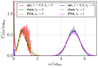
Figure 1: Comparison between the spin noise $C_{2}(\omega)$ for different approaches: solid lines represent the quantum mechanical simulation with three $I=9/2$ nuclear spins, the dashed lines are a classical simulation and the dotted lines are calculated from a Fourier transformed FOA.

To set the stage for higher order spin correlation functions, we revisit the second order spin noise $C_{2}(\omega)$ first. A basic understanding of spin noise was achieved when using the Fourier transform of the frozen Overhauser field approximation (FOA) Merkulov et al. (2002). The spin noise spectrum was extracted analytically for $b_{x}=0$ and numerically calculated for arbitrary magnetic fields. It was amply discussed in Refs. Glasenapp et al. (2016); Hackmann and Anders (2014); Hackmann et al. (2015); Uhrig et al. (2014). In Fig. 1 we provide a comparison of our two methods with this analytic approximation. The quantum mechanical and the classical simulations show good agreement with the solution of the FOA for $b_{x}=5$. The deviations of the quantum mechanical result are related to the small number of simulated bath spins. At $b_{x}=0$, the full spin rotational invariance introduces degeneracies in the eigenenergies leading to a reduction of the excitation spectrum. Therefore, the $N_{a}=32$ different sets of hyperfine coupling constants are insufficient, and the distinct nuclear frequency peaks are visible in the spectrum. This is substantially different at finite $b_{x}=5$ where these degeneracies are lifted by the Zeeman splitting, leading to an almost smooth spectrum. The classical simulation traces the Gaussian envelope of the quantum mechanical spectrum and also differs from the FOA at $b_{x}=0$. This is due to the nuclear spin dynamics included in Eq. (11) that causes an additional long-time decay in the time domain not included in the FOA. Therefore, spectral weight shifts from the delta-peak at $\omega=0$ to the Gaussian as the non-decaying fraction of $\langle S_{z}(t)S_{z}(0)\rangle$ decreases.

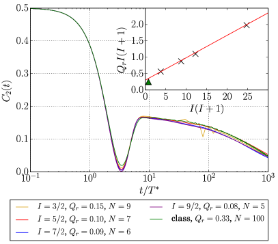
Figure 2: The second order spin correlation in the absence of an magnetic field computed by a Lanczos algorithm, with different spin lengths $I$, bath sizes $N$ and interaction strengths $Q_{r}$, chosen for similar long time decay. The inset plot shows the dependence of $Q_{r}I(I+1)$ on the squared spin length $I(I+1)$. The hyperfine couplings are homogeneous.

When adding the quadrupolar coupling to the central spin model, it is important to understand its influence on the long-time decay of $C_{2}(t)$ as a function of the bath spin length as well as number of nuclear spins in the simulation. The relative strength $Q_{r}$ defined in Eq. (32) has been originally introduced in Ref. Hackmann et al. (2015) to minimize this dependency. Since there is clear experimental evidence Hackmann et al. (2015); Bechtold et al. (2016) that $H_{Q}$ induces a second long-time decay of $C_{2}(t)$ which occurs on time scales of $200-600$ns depending on the growth conditions of the quantum dot ensemble, we aim for adjusting the value of $Q_{r}$ for each simulation such that $C_{2}(t)$ remains invariant under the change of the bath size or the spin length in order to maintain a close connection between our simulations and the experiments. By establishing this gauge we are able to compare the differences in the fourth order spectra with different bath spin lengths $I$ as well as to link the quantum and the classical simulation.

Figure 2 depicts the second-order correlation function $C_{2}(t)$ for different $I$ but similar Hilbert space dimensions $\mathcal{D}$, with a different but properly adjusted $Q_{r}$. To make sure that only the quadrupolar interaction influences the long-time dephasing for $t\gg T^{*}$, homogeneous coupling constants $A_{k}=\mathrm{const}.$ were chosen. Without quadrupolar interaction the dynamics is equivalent to the FOA for $b_{x}=0$.

For $I=3/2$, the quadrupolar coupling strength is set to $Q_{r}=0.15$, since this value has been successfully used to model experimental data Hackmann et al. (2015); Fröhling and Anders (2017). $Q_{r}$ were chosen for $I=5/2,\,7/2$ and $9/2$ (marked by ’x’ in the inset of Fig. 2) so that all correlation functions exhibit a similar long-time decay. Interestingly, the $Q_{r}$ that achieve this agreement of $C_{2}(t)$ for these different combinations of $I$ and $N$ obey the relation

$$Q_{r}I(I+1)=aI(I+1)+b,$$ (35)

with $a=0.068\pm 0.002$ and $b=0.30\pm 0.03$ obtained via linear regression. The classical computations of $C_{2}(t)$ that have been made for an effective spin vector length of $I=1/2$ follow this relation roughly (marked by a triangle in the inset plot).

V.3 Fourth-order spin noise in the CSM

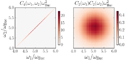
Figure 3: $C_{4}(\omega_{1},\omega_{2})$ and $C_{2}(\omega_{1})C_{2}(\omega_{2})$ as the result of a classical simulation. The cumulate $S_{4}$ spectrum is shown in Fig. 7. The external magnetic field is $b_{x}=5$.

A comparison of the quantum mechanical and classical simulation results for the fundamental features of the fourth order cumulant $S_{4}$ is the topic of this section. We discuss how the shape of $S_{4}$ is determined by its components $C_{4}$ and $C_{2}$ as well as the dependence of the spectrum on $\vec{b}_{\mathrm{ext}}$. The classical simulation is presented as a limiting case to the quantum mechanical calculation. To set the stage we limit ourselves for now to the CSM which excludes the quadrupolar interaction.

V.3.1 Components of $S_{4}$ depending on external magnetic field strength

Each $S_{4}$ spectrum consists of two parts: $C_{4}(\omega_{1},\omega_{2})$ and the product $C_{2}(\omega_{1})C_{2}(\omega_{2})$, cf. Eq. (28). The results of the classical simulation for $b_{x}=5$ are depicted in Fig. 3. Since both terms only contain quadratic expressions, their individual contributions are positive.

$C_{2}(\omega)$ is to good approximation a Gaussian with the mean given by $\sqrt{b_{x}^{2}+1/2}$, cf. Hackmann and Anders (2014), and its variance $\sigma^{2}$ is determined by the Fourier transform of the envelope of the central spin dynamics in the time domain for large magnetic fields $(\omega_{\mathrm{fluc}}/2)^{2})$ Merkulov et al. (2002). Since $\omega_{1}$ and $\omega_{2}$ are independent variables, the covariance is the identity matrix in the multivariate Gaussian given by $C_{2}(\omega_{1})C_{2}(\omega_{2})$ as shown in the right panel of Fig. 3.

$C_{4}(\omega_{1},\omega_{2})$ is plotted in the left panel of Fig. 3. It only contributes on the diagonal $\omega_{1}=\omega_{2}$. This fact is intuitively accessible in the classical approach. In each configuration the hyperfine interaction changes the initial frequency given by the generated Overhauser field only marginally. Therefore, the Fourier transform of $C_{2}^{i}(t)$ can be described by a narrow peak and the product of two distributions can only be non-zero at the overlap. For better visibility the delta-peaks are broadened to a Lorentzian with a width of $\gamma T^{\ast}=0.01$. In the direction of the diagonal, the spectrum follows a Gaussian distribution $\mathcal{N}(\sqrt{b_{x}^{2}+1/2},(\omega_{\mathrm{fluc}}/2)^{2})$. This agrees with the result of FOA Merkulov et al. (2002), since a high magnetic field suppresses spin flips, leading to an Ising model and which features a Gaussian distribution of polarization due to the central limit theorem.

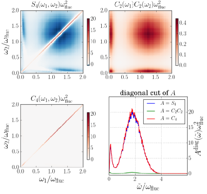
Figure 4: $S_{4}(\omega_{1},\omega_{2})\omega_{\mathrm{fluc}}^{2}$ as well as $C_{4}(\omega_{1},\omega_{2})\omega_{\mathrm{fluc}}^{2}$ and $C_{2}(\omega_{1})C_{2}(\omega_{2})\omega_{\mathrm{fluc}}^{2}$ for $b_{\mathrm{ext}}^{x}=1$ in the classical simulation with $N=100$ bath spins. In the lower right panel the diagonal cut through all three spectra is shown.

Combining the two contributions $C_{4}(\omega_{1},\omega_{2})$ and $C_{2}(\omega)$ leads to dominating correlations on the diagonal $\omega_{1}=\omega_{2}$ as well as anticorrelations elsewhere in the $(\omega_{1},\omega_{2})$-plane as a consequence of the subtraction of both terms in Eq. (22).

To parametrize the diagonal cut we define $S_{4}^{\text{diag}}(\tilde{\omega})=S_{4}(\tilde{\omega}/\sqrt{2},\tilde{\omega}/\sqrt{2})$ and plot $S_{4}^{\text{diag}}(\tilde{\omega})$ in the lower right panel of Fig. 4. For small magnetic fields the spectrum changes distinctively, as can be seen in Fig. 4. Again we find a Gaussian centred around $\sqrt{b^{2}_{x}+1/2}$ with a variance of $(\omega_{\mathrm{fluc}}/2)^{2}$ but with reduced spectral weight. For $b_{x}=0$ the correlator $C_{2}$ features a strongly pronounced delta-peak at $(\omega_{1},\omega_{2})=(0,0)$, as seen in Fig. 1, with a maximum weight of one third of the total spectral weight in the case of homogeneous coupling constants Merkulov et al. (2002). Increasing the strength of the external magnetic field not only shifts the position of the Gaussian depending on the external magnetic field but also transfers the weight of the delta-peak to the Gaussian. For higher magnetic fields, e. g. $b_{x}=5$, the contribution at $(0,0)$ has vanished, and only the Gaussian remains. The same behavior also influences the $C_{4}$ part of the spectrum, where we can observe a not yet disappeared delta-peak at the origin of coordinates for $b_{x}=1$.

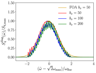
Figure 5: $S^{\text{diag}}_{4}(\tilde{\omega})$ for high ($b_{x}=50,100,200$) transversal magnetic fields. Computed via the quantum mechanical scheme for $N=3$ bath spins with a spin length of $I=9/2$. The spectra are shifted by $\sqrt{2}\omega_{\mathrm{max}}=\sqrt{2}\sqrt{b_{x}^{2}+1/2}$. The frozen Overhauser field approximation (FOA) is included for comparison.

After establishing the qualitative features of $C_{4}$ as well as the product $C_{2}C_{2}$ for smaller and intermediate transversal field strength $b_{x}$ by the classical simulation, we compare these results with the quantum mechanical calculations for a very small bath but with large nuclear in $I=9/2$ along the diagonal $\omega_{1}=\omega_{2}$.

$S_{4}^{\text{diag}}(\tilde{\omega})$ for high magnetic fields is shown in Fig. 5. The definition can be used analogously for the diagonal cuts through the $C_{2}(\omega_{1})C_{2}(\omega_{2})$ and $C_{4}(\omega_{1},\omega_{2})$ spectra. While the quantum mechanical spectra is centred around $\sqrt{b_{x}^{2}+1/2}$ at all magnetic fields and is tracing the Gaussian envelope established in the classical simulation for smaller fields, it develops a comb of peaks at high magnetic fields. At larger fields, spin-flip processes are suppressed, and the dynamics becomes increasingly dominated by the Ising part of the CSM in $x$-direction. The peak location is governed by the hyperfine interaction, with the distance decreasing with increasing bath sizes, $\propto 1/\sqrt{N}$. The width of the peaks relates to the variability of the $A_{k}$. This phenomenon can not be observed with a classical computation, where higher magnetic fields only shift the spectrum which maintains its continuous shape. With higher numbers of bath spins and a distribution of $A_{k}$ with high variability, the quantum mechanical spectrum would approach the results of the classical simulation.

V.3.2 Classical simulation as a limiting case of the quantum mechanical treatment of $S_{4}$

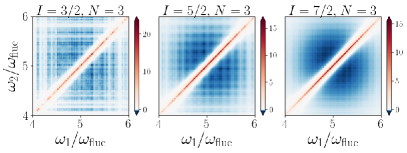
Figure 6: $S_{4}(\omega_{1},\omega_{2})$ computed for a bath size of $N=3$ with spin lengths $I=3/2$, $I=5/2$ and $I=7/2$ and an $A_{k}$ configuration with $r_{0}=0.8$. The transversal magnetic field is set to $b_{x}=5$, and quadrupolar interaction is switched off.

While the classical approach always yields a continuous frequency spectrum, the variation of nuclear spin length as well as the bath size merits a more in-depth investigation for the quantum mechanical simulation.

Figure 6 shows the quantum mechanical results for $S_{4}(\omega_{1},\omega_{2})$ obtained by Eq. (28) for different spin lengths ($I=3/2,\,5/2,\,7/2$) and a fixed number of bath spins ($N=3$) in a transversal field $b_{x}=5$ applying an average over $N_{a}=32$ configurations of $\{A_{k}\}$. The spectrum becomes more continuous with a growing spin length, due to the exponential increase in the Hilbert space dimension and the larger number of non-degenerate eigenenergies. As seen in the left panel of Fig. 6, the non-zero contributions to $S_{4}$ are concentrated at a sparse number of $(\omega_{1},\omega_{2})$ frequency pairs for $N=3$ $I=3/2$-spins, due to the limitations of the energy excitation spectrum. The delta-peaks in Eq. (28) are broadened by a factor $\gamma T^{\ast}=0.01$. Correlations (red) are restricted to the frequency subspace $\omega_{1}=\omega_{2}$, while the anti-correlations (blue) can be found in an area centered around $\omega_{1}=\omega_{2}\approx b_{x}$. Note the similarity between the classical results (Fig. 7, lower right panel) and the quantum mechanical solution for $N=3$ and $I=7/2$ (Fig. 6, right panel), solidifying the conjecture that the quantum mechanical spectra approaches the results of the classical simulation in the limit of $I\to\infty$.

The fourth-order cumulant spectra $S_{4}(\omega_{1},\omega_{2})$ are presented for different $N$ and a fixed spin length $I=9/2$ at $b_{x}=5$ in Fig. 7. For $N=1$, the position of the non-zero contributions are clearly governed by the Zeeman splitting of the nuclear spins coupled to the central spin via a single hyperfine coupling constant $A=\omega_{\rm fluc}$. This results in $(2I+1)^{2}$ equidistant peaks on a grid around the point given by $(\omega_{L},\omega_{L})$, that are positive at the $\omega_{1}=\omega_{2}$ diagonal and negative everywhere else. For larger bath sizes the spectrum becomes more continuous. At $N=3$ bath spins of length $I=9/2$ the $S_{4}$ spectrum, as displayed in the lower left panel of Fig. 7, is already qualitatively very similar to the classical result depicted on the lower right panel of Fig. 7.

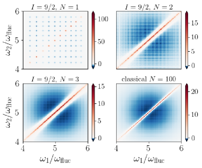
Figure 7: $S_{4}(\omega_{1},\omega_{2})$ computed for $N=1,2,3$ bath spins with $I=9/2$, and for $N=100$ classical spins. The transversal magnetic field is $b_{x}=5$, and quadrupolar interaction is not included.

The simulations show that the classical calculations are valid limits of the quantum mechanical calculations for $I\rightarrow\infty$ and $N\rightarrow\infty$. Furthermore, we established that fourth order cumulant does not vanish implying that the central spin does not behave as a classical random variable whose noise spectrum is purely of Gaussian type. The physics is driven by the coherent precession around the external constant magnetic field in combination with a slowly varying nuclear spin dynamics. The FOA reveals the restriction of $C_{4}$ to the frequency diagonal which is shared by both approaches that explicitly include the nuclear spin dynamics.

V.4 Influence of quadrupolar interaction on $S_{4}(\omega_{1},\omega_{2})$

Within the CSM, the positive correlations are restricted to the diagonal $\omega_{1}=\omega_{2}$ related to the spectral confinement of $C_{4}(\omega_{1},\omega_{2})$ leading to anti-correlation everywhere else in the frequency plane. In this section, we add the nuclear-electric quadrupolar interaction $H_{Q}$ to the CSM and investigate its influence onto $S_{4}$.

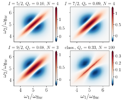
Figure 8: $S_{4}/\omega_{1},\omega_{2})$ with a magnetic field $b_{\mathrm{ext}}^{x}=5$, with different spin lengths $I$, bath sizes $N$ and interaction strengths $Q_{r}$. The parameters are chosen for similar behavior in the second order spin correlation, see Fig. 2.

V.4.1 Fourth-order spin noise at intermediate and large magnet fields

Here, we focus on intermediate and large magnet fields since in this regime the spin-noise power spectrum $C_{2}(\omega)$ remains unaltered in the presence of quadrupolar interaction. In leading order $C_{2}(\omega)$ is described by a Gaussian Merkulov et al. (2002); Glazov and Ivchenko (2012) centered around $\omega_{1}$ – see also Sec. V.2.

Figure 8 shows $S_{4}(\omega_{1},\omega_{2})$ computed quantum mechanically for bath spin lengths $I=3/2,\,7/2,\,9/2$ as well as the results of the classical approach. The strength of the quadrupolar coupling is chosen such that $C_{2}(t)$ agrees for $b_{\text{ext}}=0$ independent of the spin length – see the discussion in Sec. V.2. While the fourth-order contribution to $S_{4}$ is restricted to the diagonal, $\omega_{1}=\omega_{2}$ without quadrupolar interaction, the introduction of quadrupolar couplings causes a broadening of the heretofore sharp peak. But while the quantum mechanical cumulant spectra look very similar, the classically computed $S_{4}$ exhibits a much smaller broadening of the positive contribution around $\omega_{1}=\omega_{2}$, and a qualitatively different peak shape as can be seen in the lower right panel of Fig. 8. Since the quadrupolar interaction does not affect the shape of $C_{2}(\omega)$ for transversal magnetic fields $b_{x}>1$ in both approaches, the mismatch between quantum mechanical and classical fourth-order cumulant is related to $C_{4}$.

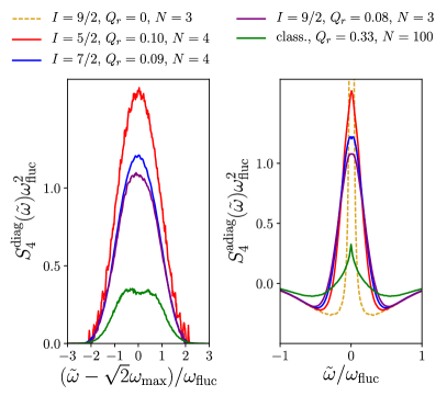
Figure 9: The same data plotted in Fig. 8, cut in the diagonal $\omega_{1}=\omega_{2}$, $S_{4}^{\text{diag}}(\tilde{\omega})$, as well as in the anti-diagonal cut $\omega_{1}+\omega_{2}=2\omega_{\mathrm{max}}$, $S_{4}^{\text{adiag}}(\tilde{\omega})$. $S_{4}^{\text{diag}}(\tilde{\omega})$ without quadrupolar coupling was added in the right panel for comparison.

To further investigate the broadening of the correlation caused by quadrupolar coupling, especially how this broadening behaves dependent on the $Q_{r}$, we analyze the broadening of $C_{4}$ perpendicular to the frequency diagonal as function of $Q_{r}$. For that purpose, we parametrize the anti-diagonal cut in the vicinity of its global maximum, $S_{4}(\omega_{\text{max}},\omega_{\text{max}})$, with $\omega_{\text{max}}/\omega_{\text{fluc}}=\sqrt{b^{2}_{x}+1/2}$ by $\omega_{1}+\omega_{2}=2\omega_{\text{max}}$. We define the corresponding anti-diagonal cut as

$$S_{4}^{\text{adiag}}(\tilde{\omega})=S_{4}\left(\omega_{\text{max}}+\frac{\tilde{\omega}}{\sqrt{2}},\omega_{\text{max}}-\frac{\tilde{\omega}}{\sqrt{2}}\right)$$ (36)

so that the global maximum is located at the relative frequency $\tilde{\omega}=0$.

The diagonal and anti-diagonal cuts of the data presented in Fig. 8 are plotted in Fig. 9. The same parameters that produced congruent results for conventional spin noise spectrum $C_{2}(\omega)$ as shown in Fig. 1, now lead to markedly different behaviour. The left panel shows the diagonal cuts computed with the quantum mechanical method for different nuclear spin length I and bath size $N$ and is augmented by the results of the classical approach for $N=100$ nuclear spins. The diagonal cuts exhibit roughly the same Gaussian behaviour independent of $Q_{r}$, but its amplitude decreases by about a factor five. This is a direct result of the broadening observed in Fig. 8, as the total spectral weight of $C_{4}$ as well as $S_{4}$ remains conserved. The drop in amplitude is not uniform, but is more pronounced in $S_{4}$ computed via the classical approach, suggesting that the quadrupolar coupling has a stronger effect there. In the quantum mechanically computed $S_{4}$ the amplitude decreases with larger $I$.

On the right panel of Fig. 9 the anti-diagonal cuts are shown for the same parameters as in the left panel. Added for comparison is $S_{4}^{\text{adiag}}(\tilde{\omega})$ for $Q_{r}=0$ obtained with the same broadening parameter $\gamma$. $S_{4}^{\text{adiag}}(\tilde{\omega})$ reveals a fundamentally different curve shape depending on the computational approach. While the classical curve exhibits a cusp which could be fitted by a power law, the quantum mechanical approach yields a Gaussian shape.

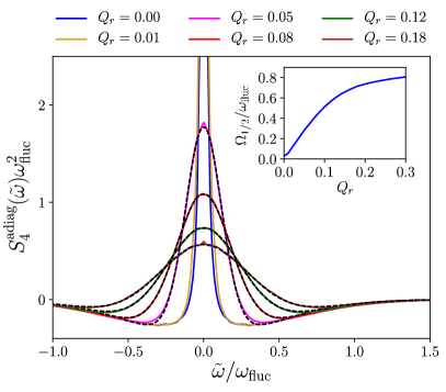
Figure 10: $S_{4}^{\text{adiag}}(\tilde{\omega})$ quantum mechanically calculated with $N=3$, $b_{x}=5$ and $I=9/2$ for different $Q_{r}$. The inset plot shows the full width half maximum $\Omega_{1/2}$ of $C_{4}$ in relation to the quadrupolar coupling strength $Q_{r}$.

The scaling behavior which allows us to match classical and quantum mechanical results for $C_{2}(\omega)$ by adjusting $Q_{r}$, cf. Sec. V.2, therefore only holds for the second order spin noise and not the fourth order spin-noise bispectrum. It stands to reason that the quantum mechanical method includes features that have been neglected in the classical approach, such as the non-commutability of the bath spin components.

In order to connect the relative quadrupolar coupling strength $Q_{r}$ with the broadening of the anti-diagonal, we plotted $S_{4}^{\text{adiag}}(\tilde{\omega})$ for different $Q_{r}$ and fixed $N=3$ and $I=9/2$ in Fig. 10. The contribution $C_{2}(\omega_{1})C_{2}(\omega_{2})$, can be represented by a Gaussian with the variance $\sigma^{2}=(\omega_{\mathrm{fluc}}/2)^{2}$ independent of $Q_{r}$ compatible with the FOA Merkulov et al. (2002). The fourth-order contribution $C_{4}$ in contrast changes markedly with the quadrupolar interaction strength. Fitting only $C_{4}$ with a Gaussian leads to the relation between the full-width half maximum $\Omega_{1/2}$ and the quadrupolar coupling strength $Q_{r}$ shown in the inset of Fig. 10. For small $Q_{r}$, the dependence is roughly linear, before the increase flattens at $Q_{r}>0.1$. For $Q_{r}\rightarrow 0$, the Gaussian curve becomes a sharp peak $\Omega_{1/2}\rightarrow 0$ limited here due to the Lorentz broadening simulating a finite measuring time $T_{m}$.

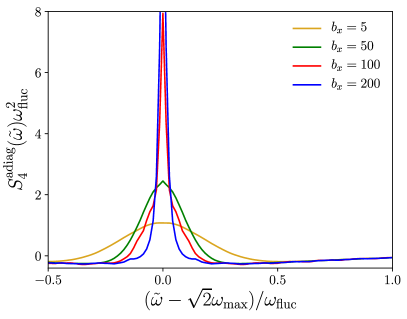
Figure 11: $S_{4}^{\text{adiag}}(\tilde{\omega})$ quantum mechanically calculated with $N=3$, $Q_{r}=0.08$ and $I=9/2$ for different transversally applied external magnetic fields $b_{x}$.

Figure 11 depicts the anti-diagonal cut $S_{4}^{\text{adiag}}(\tilde{\omega})$ for different magnetic fields $b_{x}$ and fixed spin bath size and spin length. The quadrupolar coupling induced broadening decreases with an increasing magnetic field strength: the dynamics of the system is dominated by the Zeeman energy, and $H_{Q}$ becomes an increasingly weaker perturbation. This agrees well with the observation of the fourth-order spin correlation function in the time domain Fröhling and Anders (2017), where the high magnetic fields shift the decay time from $\mathcal{O}(\mathrm{ns})$ to an exponential decay with a magnetic field dependent decay time $T_{2}\propto\mathcal{O}(\mu\mathrm{s})$ Press et al. (2010); Bechtold et al. (2016, 2015).

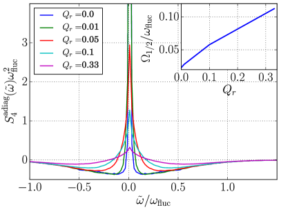
Figure 12: Cuts for the classically calculated $S_{4}^{\text{adiag}}(\tilde{\omega})$. The inset plot shows the full width at half maximum $\Omega_{1/2}$ of the $C_{4}$ part dependent on the quadrupolar coupling strength $Q_{r}$.

We performed the same type of simulations as in Fig. 10 using the classical approach. Figure 12 shows $S_{4}^{\text{adiag}}(\tilde{\omega})$ for different $Q_{r}$. Since $C_{2}(\omega)$ remains invariant under the change of $Q_{r}$, the change in the spectrum is directly linked to the change of $C_{4}(\omega_{1},\omega_{2})$. As in the quantum mechanical simulations, the quadrupolar interaction lifts the spectral constrain to $\omega_{1}=\omega_{2}$ in $C_{4}(\omega_{1},\omega_{2})$. The overall sum-rule for $C_{4}(\omega_{1},\omega_{2})$ implies a decrease of the peak at $\tilde{\omega}=0$ and an increasing distribution of spectral weight into the $(\omega_{1},\omega_{2})$ plane. Since the shape of the classical $S_{4}^{\text{adiag}}(\tilde{\omega})$ is non-Gaussian, we extracted the full-width half maximum $\Omega_{1/2}$ of $C_{4}$ as function of $Q_{r}$ and plotted the result as inset in Fig. 12. In full agreement with the quantum mechanical approach we find a linear dependency of $\Omega_{1/2}$ on $Q_{r}$. The finite offset at $Q_{r}=0$ is related to the finite size effect of the Fourier transformation for $T_{m}<\infty$. The absolute value of $\Omega_{1/2}$, however, differs between the quantum mechanical and the classical simulations which we attribute to the bath size difference.

V.4.2 Fourth-order spin noise in the crossover regime

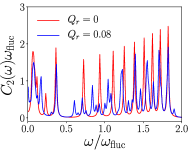
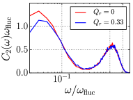
Figure 13: Comparison of $C_{2}(\omega)$ with and without $H_{Q}$. The left panel shows the results of quantum mechanical calculation, with $N=1$, $I=9/2$ and $Q_{r}=0.08$, the right panel the classically computed spectrum using $N=100$, $Q_{r}=0.33$.

Now we turn to the crossover regime where the Zeeman energy is of the order of $\omega_{\rm fluc}$, i. e. $b_{x}\approx 1$. The electron spin dynamics is governed by the external magnetic field and the fluctuating Overhauser field which have equal strength. Furthermore, the nuclear Zeeman energy is weak such that the nuclear spin dynamics is dominated by the nuclear-electric quadrupolar interaction in combination with the weak Knight field generated by the electron spin. We are interested in comparing two extreme limits: the dynamics of the smallest system one can imagine, including only a single nuclear spin, and the limit of large number of spins. While $N=1$ requires a purely quantum mechanical calculations, we mimic the large N limit with a classical simulation of $N=100$ bath spins.

In this regime $H_{Q}$ does not only influence $S_{4}$ but also modifies $C_{2}(\omega)$. The change of $C_{2}(\omega)$ induced by the quadrupolar interaction is depicted in Fig. 13 for bath sizes $N=1$ (left panel) and $N=100$ (right panel).

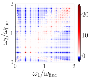
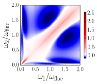
Figure 14: $S_{4}$ for a smaller magnetic field of $b_{x}=1$. Left is the quantum mechanical calculation, with $N=1$, $I=9/2$ and $Q_{r}=0.08$. On the right is the classically computed spectrum with $N=100$, $Q_{r}=0.33$.

We use the corresponding spin noise $C_{2}$ to calculate the fourth order cumulant. In Fig. 14 the classical and the quantum mechanical results of $S_{4}$ are presented for $b_{x}=1$. Note that the quantum mechanical $S_{4}$ on the left computed in the limit of weak measurement for $N=1$, is near identical to the $S_{4}$ presented for strong and continuous measurement in Ref. Hägele and Schefczik (2018). For small $\omega_{1}$ or $\omega_{2}$ we also found alternating signs of correlations in the $(\omega_{1},\omega_{2})$-plane. Fixing $\omega_{1}/\omega_{\rm fluc}=1$ and increasing $\omega_{2}$ reveals first weak anti-correlation (encoded in blue), then correlations (encoded in red) before switching back to anti-correlations. Also, the strong correlations are not confined to the diagonal as depicted in Fig. 7 but are significantly spread due to the presence of the quadrupolar couplings.

The classically obtained $S_{4}$ on the right shows the effects of quadrupolar coupling in small magnetic fields for a far bigger bath of $N=100$, which results in a continuous spectrum with similar features. These are the anti-correlation contributions at the axis with a dip in anti-correlation along $\omega_{1/2}/\omega_{\rm fluc}=1$, as well as the broadening of the correlation on the diagonal.

V.4.3 Discussion

While the second-order spin correlation function $C_{2}(t)$ decays fast on the time scale $T^{*}$ in finite magnetic field that long-time effects of nuclear quadrupolar coupling cannot be observed in the electron spin dynamics, they modify the frequency characteristics of the fourth-order spin correlation function significantly. The positive correlations in the spin noise power bispectrum that are pinned to the frequency diagonal in the CSM are broadened and acquire a finite width proportional to the nuclear coupling strength at a large magnetic field.

With and without quadrupolar interaction the classical and the quantum mechanical method yield congruent results for the second-order correlation. The same is true for the fourth-order correlation without quadrupolar interaction. If quadrupolar interaction is introduced, both the classical and quantum mechanical method show qualitatively similar behavior - a broadening of the correlation peak along the $\omega_{1}+\omega_{2}=\mathrm{const}$ cut. But, as can be seen in Fig. 9, the spectra of different methods exhibit a quantitatively different curve progression, and to not follow the same scaling behavior presented in Sec. V.2. This shows that the fourth-order correlation yields uniquely quantum mechanical information that appears with the introduction of quadrupolar interaction into the system, as has been previously shown in Fröhling and Anders (2017).

It is straight forward to extend the investigation to an arbitrary angle between the $z$-axis and the applied magnetic field. This is a well studied problem in the context of the standard SNS and it turns out that a tilted magnetic field does not provide additional new information. Therefore, we do not include these results in this paper. For the limiting case of a single bath spin, i. e. $N=1$, we refer to Fig. 6 in Ref. Hägele and Schefczik (2018) which extrapolated to continuous spectra as obtained with our classical simulation.

VI Conclusion

We presented a combination of a quantum mechanical and a classical simulation to the fourth order noise correlation function, to calculate the spin-noise power bispectrum in a quantum dot in the presence of the nuclear-electric quadrupolar interaction in the limit of a very small and a very large nuclear spin bath. Our approach is valid in the limit of a nearly perturbation free off-resonance detection of the spin polarisation in the quantum dot ensemble using the Faraday rotation of a weak linear polarized optical probe signal.

The second-order spin correlation function $C_{2}(t)$ is used as a gauge to connect the nuclear spin length $I$ and the effective quadrupolar interaction strength $Q_{r}$ to the number of nuclear spins of the spin bath in all calculations. To account for the effect of quadrupolar interaction in a classical spin dynamics, we derived a modification of the effective Knight field in classical equations of motions.

The quantum mechanical and the classical spin-noise bispectrum agree well for the CSM. The quantum mechanical bispectrum converges to the result of the classical simulation for large nuclear spin bath and large nuclear spin length. In both cases the quantum mechanical eigenvalue spectrum approaches a continuum distribution. Interestingly, already relatively small spin baths provide a good representation of a larger bath bispectrum.

The fourth order cumulant $S_{4}$ is made up of two basic building blocks: $C_{4}(\omega_{1},\omega_{2})$ and $C_{2}(\omega_{1})C_{2}(\omega_{2})$. The decomposition of those parts show that the product of the second-order spin noise gives a 2D Gaussian which is solely responsible for anti-correlation in the spectrum while $C_{4}$ is non-zero only on the diagonal in the CSM.

Adding the quadrupolar interaction term $H_{Q}$ to the CSM is causing a broadening of $C_{4}$ across the diagonal. The width of this broadening is directly proportional to the quadrupolar coupling strength at small couplings and a finite magnetic field. The width could be used as a direct experimental probe of the average quadrupolar interaction strength in a sample. The near perfect agreement observed in $C_{2}(\omega)$ between the classical and the quantum mechanical simulations is slightly modified in the bispectrum. The qualitative agreement between the bispectra of both methods with comparable parameters is remarkable concerning the location of the correlation as well as the anti-correlations. The broadening of the quantum mechanical spectra $C_{4}$ along the diagonal, however, is more pronounced than in its classical counterpart, while the decrease of the amplitude due to quadrupolar interaction is stronger for the results of the classical method. The difference in the shape between the results of both methods becomes visible in the cut through the diagonal.

We have proven that the simple linear response theory to higher correlation functions Li et al. (2013); Li and Sinitsyn (2016) produces congruous results to those obtained with an elaborate weak measurement theory presented in Ref. Hägele and Schefczik (2018). This shows that the assumption of a non-perturbative measurement yields identical results that the weak measurement theory in the weak coupling limit Hägele and Schefczik (2018).