Quantum speed limit time for correlated quantum channel

Abstract

Memory effects play a fundamental role in the dynamics of open quantum systems. There exist two different views on memory for quantum noises. In the first view, the quantum channel has memory when there exist correlations between successive uses of the channels on a sequence of quantum systems. These types of channels are also known as correlated quantum channels. In the second view, memory effects result from correlations which are created during the quantum evolution. In this work we will consider the first view and study the quantum speed limit time for a correlated quantum channel. Quantum speed limit time is the bound on the minimal time which is needed for a quantum system to evolve from an initial state to desired states. The quantum evolution is fast if the quantum speed limit time is short. In this work, we will study the quantum speed limit time for some correlated unital and correlated non-unital channels. As an example for unital channels we choose correlated dephasing colored noise. We also consider the correlated amplitude damping and correlated squeezed generalized amplitude damping channels as the examples for non-unital channels. It will be shown that the quantum speed limit time for correlated pure dephasing colored noise is increased by increasing correlation strength, while for correlated amplitude damping and correlated squeezed generalized amplitude damping channels quantum speed limit time is decreased by increasing correlation strength.

1 Introduction

It is impossible to isolate a quantum system from its surroundings leading to information loss in the form of dissipation and decoherence. The theory of open quantum systems offers the necessary tools for describing and analyzing the interactions of a system with its surrounding Breuer . In the theory of open quantum systems, various methods have been proposed to illustrate the environment and its effects on the dynamics of the desired system Breuer ; Weiss . If the coupling strength between the system and the environment is weak and the relaxation time of the system is longer than correlation time of the environment, then there exist a one-way flow of information from the system to the environment. Such a quantum evolution is called Markovian Gorini and it can be described by the master equation in Lindblad form Lindblad ; Zhang1 ; Carmichael . In a more realistic situation, the coupling strength between the system and the environment is strong and the relaxation time of the system is shorter than the correlation time of the environment. In this case there exist a back-flow of information from environment to the system. This type of quantum evolution is called non-MarkovianWolf ; Rivas ; Rivas1 ; Haseli ; Haseli1 ; Haseli2 ; Fanchini . In the theory of open quantum systems, dynamical memory effects play a fundamental role in various physical phenomena such as quantum biology Lambert ; Thorwart ; Huelga , quantum cryptography Vasile , quantum metrology Chin and quantum control Hwang . According to the types of dynamical memory effects, quantum evolutions can be divided into two categories: memory-less evolution (Markovian evolution) and quantum process with memory (non-Markovian evolution). In the case of non-Markovian evolution, future states of a system can be depend on its past because of the back-flow of information . So it is natural to conclude that the back-flow of information from the environment to the system has a direct relation to the existence of memory.

This view about the dynamical memory effects and non-Markovianity as a typical part of the theory of open quantum systems is completely different from the concept of quantum channels with memory. In order to distinguish between these two, the term "correlated quantum channel" is used to describe quantum channels with memory. The memory of the quantum channel is depicted by successive uses of the channels on a sequence of quantum systems Macchiavello ; Caruso ; Kretschmann . In this sense, channels with memory and without memory channels represent cases in which the successive uses of the channels are correlated or independent, respectively. In the case of a correlated quantum channel, memory is not due to the correlations created during the time evolution but due to the correlated action of channels on the system consisting of a set of individual quantum systems. Addis et al. have studied the connection between these two insight about memory in Ref. Addis .

The dynamics of quantum correlations under correlated quantum channels has been studied previously. In Ref. Ramzan , the effects of correlated quantum channels have been investigated on the entanglement of $X$-type state of the Dirac fields in the non-inertial frame. In Ref. Guo , the authors have shown that how the correlated channel affects the dynamics of quantum correlations. The behavior of memory-assisted entropic uncertainty relation under the effects of the correlated quantum channels has been investigated in Refs. Karpat ; Guo1 .

We study the quantum speed limit QSL time for correlated and uncorrelated quantum channels. QSL time is the bound on the minimal time which is needed for a quantum system to evolve from an initial state at initial time $\tau$ to desired states at time $\tau+\tau_{D}$, where $\tau_{D}$ is the driving time. In Ref.Mandelstam , Mandelstam and Tamm have provided a bound for closed quantum systems which is given by

$$\tau\geq\tau_{QSL}=\frac{\pi\hbar}{2\Delta E},$$ (1)

where $\Delta E=\sqrt{\langle\hat{H}^{2}\rangle-\langle\hat{H}\rangle^{2}}$ is the inverse of the variation of energy of the initial state and $\hat{H}$ is time-independent Hamiltonian describing the dynamics of quantum system. This bound is known as the MT bound. Margolus and Levitin have presented the bound for closed quantum system based on the mean energy $E=\langle\hat{H}\rangle$ as Margolus

$$\tau\geq\tau_{QSL}=\frac{\pi\hbar}{2E},$$ (2)

which is called the ML bound. Combining the MT and ML bounds in Eqs. (1) and (2) provides a unified bound for the QSL time for the dynamics of closed quantum system as Giovannetti

$$\tau\geq\tau_{QSL}=\max\{\frac{\pi\hbar}{2\Delta E},\frac{\pi\hbar}{2E}\}.$$ (3)

Recently, QSL time has also been studied for the dynamics of open quantum systems which are described by positive non-unitary maps. For open quantum systems QSL time has quantified based on quantum Fisher information Taddei ; Escher , Bures angle Deffner1 , relative purity del ; Zhang and other proper geometric approach Xu ; Mondal ; Levitin ; Xu1 ; Meng ; Mirkin ; Campaioli ; Uzdin .

In this work, we will show how correlations in the application of quantum channels can effect QSL time. We provide results for some unital and non-unital correlated channels. We will consider random dephasing correlated noise as an example for unital correlated quantum channels and consider correlated amplitude damping and correlated squeezed generalized amplitude damping channels SGAD as examples for the non-unital correlated quantum channels.

In this work, we investigate the effects of correlations in the quantum channel on QSL time, so we do not limit ourselves to choose a particular measure of QSL time. We use the bound based on relative purity for QSL time which was introduced in Zhang . We choose this bound because it can be used for arbitrary initial pure and mixed states.

This work is organized as follows. In Sec. 2 we review the geometric approaches based on relative purity for driving the QSL bounds. In Sec. 3, the QSL time for correlated and uncorrelated quantum channel is investigaed. We will consider correlated pure dephasing colored noise as an example for correlated unital channel and consider correlated amplitude damping and squeezed generalized amplitude damping SGAD channels as examples for the non-unital correlated quantum channels. In Sec. 4, we summarize the results.

2 The quantum speed limit time for open quantum system

The state of the open quantum system at time $t$ is characterized by density matrix $\rho_{t}$. Time evolution of an open quantum system is defined by the following time-dependent master equation as

$$\dot{\rho}_{t}=L_{t}(\rho_{t}),$$ (4)

where $L_{t}$ is the positive generator Breuer . The goal is to find the minimum time for evolving from the state $\rho_{\tau}$ at time $\tau$ to desire state $\rho_{\tau+\tau_{D}}$ at time $\tau+\tau_{D}$. Here, $\tau_{D}$ is the driving time of the open quantum system. Based on relative purity the QSL time has been introduced by the authors in Refs. del ; Zhang . Zhang et al. have shown that this QSL time is applicable for arbitrary initial mixed and pure states. The relative purity $f(\tau)$ between initial state $\rho_{\tau}$ and desire state $\rho_{\tau+\tau_{D}}$ is given by Audenaert

$$f(\tau+\tau_{D})=\frac{tr(\rho_{\tau}\rho_{\tau+\tau_{D}})}{tr(\rho_{\tau}^{2})}.$$ (5)

The ML bound of QSL time for open quantum systems is given by (see Ref. Zhang for details)

$$\tau\geq\frac{|f(\tau+\tau_{D})-1|tr(\rho_{\tau}^{2})}{\overline{\sum_{i=1}^{n}\Lambda_{i}\beta_{i}}},$$ (6)

where $\Lambda_{i}$ and $\beta_{i}$ are the singular values of $\mathcal{L}_{t}(\rho_{t})$ and $\rho_{\tau}$, respectively and in the denominator of the bound, we have $\overline{\square}=\frac{1}{\tau_{D}}\int_{\tau}^{\tau+\tau_{D}}\square dt$. Following the same procedure the MT bound of QSL-time for open quantum systems can be written as

$$\tau\geq\frac{|f(\tau+\tau_{D})-1|tr(\rho_{\tau}^{2})}{\overline{\sqrt{\sum_{i=1}^{n}\Lambda_{i}^{2}}}}.$$ (7)

Combining Eqs. (6) and (7) leads to a unified bound for QSL time as

$$\tau_{QSL}=\max\{\frac{1}{\overline{\sum_{i=1}^{n}\Lambda_{i}\beta_{i}}},\frac{1}{\overline{\sqrt{\sum_{i=1}^{n}\Lambda_{i}^{2}}}}\}\times|f(\tau+\tau_{D})-1|tr(\rho_{\tau}^{2}).$$ (8)

Zhang et al. have shown that the QSL-time is associated with quantum coherence of an arbitrary initial state $\rho_{\tau}$ Zhang . They have also shown that for open quantum systems the ML bound of the QSL time in Eq. (6) is tighter than MT bound. QSL time is shorter than $\tau_{D}$. It is worth noting that QSL-time $\tau_{(QSL)}$ can be interpreted as the potential capacity for further evolution acceleration. If $\tau_{QSL}=\tau_{D}$ then the evolution is now in the situation with the highest speed, thus the evolution does not have the potential capacity for further acceleration. However, when $\tau_{QSL}<\tau_{D}$, the potential capacity for further acceleration will be greater. Another important point to be noted is that when the coupling strength between the system and environment is weak $\tau_{QSL}$ tends to the actual driving time $\tau_{D}$. On the contrary, in the strong coupling limit between the system and environment, $\tau_{QSL}$ can reduce below the actual driving time $\tau_{D}$ Deffner1 .

3 Correlated quantum channels

We provide a brief review on quantum channel with correlated noise Macchiavello ; Caruso ; Kretschmann ; Addis ; Ramzan ; Guo ; Yeo ; Awasthi . Quantum channels are divided into two categories of with memory and without memory channels. If the correlation time of the environment is shorter than the time between successive application then there is no correlation between consecutive uses of the channel, i.e. a quantum channel $\varepsilon$ for $N$ consecutive uses obey $\varepsilon_{N}=\varepsilon^{\otimes N}$. These kinds of channels are known as channel without memory (uncorrelated channels). However, in real physical quantum noise, it is logical to have correlations between consecutive application of the channels. In this case, the correlation time of the environment is longer than the time between the successive application of the channels, i.e. a quantum channel $\varepsilon$ for $N$ successive uses obeys $\varepsilon_{N}\neq\varepsilon^{\otimes N}$. These kinds of channels are known as memory channels (correlated channels). For correlated channels, the channel acts dependently on each input. Here we consider $N$ consecutive uses of the quantum channel. A quantum channel $\varepsilon$ can be represented as a completely positive, trace-preserving map from input state $\rho$ to output $\varepsilon(\rho)$ in Kraus form

$$\varepsilon(\rho)=\sum_{i_{1}...i_{N}}E_{i_{1}...i_{N}}\rho E_{i_{1}...i_{N}}^{{\dagger}},$$ (9)

where $E_{i_{1}...i_{N}}$’s are Kraus operators which are defined as

$$E_{i_{1}...i_{N}}=\sqrt{P_{i_{1}...i_{N}}}A_{i_{1}}\otimes...\otimes A_{i_{N}},\quad\sum_{i}P_{i_{1}...i_{N}}=1.$$ (10)

Here $P_{i_{1}...i_{N}}$ is the probability that a random sequence of operations is acted on the sequence input $N$ qubits which are transmitted through the channel. In general, the Kraus operators for two consecutive uses of a two-qubit quantum channel can be represented as

$$E_{ij}=\sqrt{P_{ij}}A_{i}\otimes A_{j}.$$ (11)

For uncorrelated channel we have $P_{ij}=P_{i}P_{j}$ and Kraus operators are independent of each other. Whereas, for correlated channel based on Bayes rule we have $P_{ij}=P_{i}P_{j|i}$, where $P_{j|i}$ is the conditional probability. Thus, for two consecutive uses of a two-qubit quantum channel with partial correlation the Kraus operators can be represented as

$$E_{ij}=\sqrt{P_{i}[(1-\mu)P_{j}+\mu\delta_{ij}]},$$ (12)

where $\mu\in[0,1]$ defines the correlation of the quantum channel. According to the Kraus operator formalism the final state is given by

$$\varepsilon(\rho) = (1-\mu)\sum_{i,j}E_{ij}\rho E_{ij}^{{\dagger}}+\mu\sum_{k}E_{kk}\rho E_{kk}^{{\dagger}}$$ (13)

$$= (1-\mu)\varepsilon_{un}(\rho)+\mu\varepsilon_{co}(\rho),$$

where $\varepsilon_{un}$ represents the uncorrelated channel and $\varepsilon_{co}$ stands for the correlated channel. In the case $\mu=0$, there is no correlation between two consecutive uses of channel and when $\mu=1$, the channel is fully correlated. In other words, $\mu=0$ represents the channel without memory and $\mu=1$ implies the channel with memory. Note that, in all parts of this work, we will consider the following initial states

$$\rho_{0}=r|\psi\rangle\langle\psi|+\frac{1-r}{4}\mathrm{I},$$ (14)

where $|\psi\rangle=\sqrt{1-\alpha^{2}}|01\rangle+\alpha|10\rangle$, $0\leq\alpha\leq 1$ and $r$ represents the purity of the initial state.

3.1 Unital correlated channel

The completely positive trace preserving channel $\varepsilon$ is unital if it maps the identity operator $\sigma_{0}=\mathcal{I}$ to itself in the same space, i.e. $\varepsilon(\sigma_{0})=\sigma_{0}$. For single-qubit systems, the unital channel can be represented in terms of a convex combination of the Pauli operators Nielsen ; Imre ; King . From geometrical insights, the unital channels map the center of the Bloch sphere to itself. Here we consider dephasing colored noise in the category of Pauli channels as an example of an unital channel Daffer . We will study the QSL time for correlated dephasing colored noise.
Pure dephasing colored noise: Let us consider the interaction between a single-qubit system and an environment which has the property of random telegraph signal noise Daffer . The dynamics of a single-qubit is described by the time-dependent Hamiltonian

$$H(t)=\sum_{k=1}^{3}\Gamma_{k}(t)\sigma_{k},$$ (15)

where $\sigma_{k}$’s are the Pauli operators in ($x,y,z$)directions, and $\Gamma_{k}(t)$’s are random variables which follow the statistics of a random telegraph signal. $\Gamma_{k}(t)$ depends on the random variable $n_{k}(t)$ as $\Gamma_{k}(t)=\alpha_{k}n_{k}(t)$, where $n_{k}(t)$ has a Poisson distribution with an average value equal to $t/2\tau_{k}$ and $\alpha_{k}$’s are coin-flip random variables that can have values $\pm\alpha_{k}$ randomly. We have a dephasing model with colored noise if $\alpha_{1}=\alpha_{2}=0$ and $\alpha_{3}=\alpha$. In this case, the dynamics of single-qubit system can be described by the following Kraus operators

$$E_{0}=\sqrt{P_{0}}\sigma_{0},\quad E_{3}=\sqrt{P_{3}}\sigma_{3},\\$$ (16)

with $P_{0}=1-z_{t}$ and $P_{3}=z_{t}$, where $z_{t}=\frac{1-\Lambda(t)}{2}$ and $\Lambda(t)=e^{-t/2\nu}[\cos(\mu t/2\nu)+\sin(\mu t/2\nu)/\mu]$, $\mu=\sqrt{(4\nu)^{2}-1}$ . Here, the range of $\nu$ quantifies the interval in which the channel is non-Markovian. Based on the results presented in Ref. Haseli1 , the quantum evolution will be non-Markovian if $\nu\geq 1/4$.

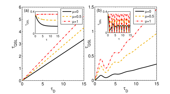
Figure 1: QSL time for correlated pure dephasing colored as a function of the driving time $\tau_{D}$ when the initial state parameters are $r=1/2$ and $\alpha=1/\sqrt{2}$ and $\tau=1$. (a)The dynamics is Markovian $\nu=0.1$ (b)The dynamics is non-Markovian $\nu=1$. The inset represents the QSL time as a function of initial time $\tau$ when $\tau_{D}=1$.

When two-qubit are transmitted through the colored pure dephasing channel, the channel with uncorrelated noise can be defined by the following Kraus operators

$$E_{ij}=\sqrt{P_{i}P_{j}}\sigma_{i}\otimes\sigma_{j},\quad i,j\in\{0,3\}.$$ (17)

In the presence of correlation between two successive uses of the colored pure dephasing channel on two-qubit system, the Kraus operators $E_{kk}$ are given by

$$E_{kk}=\sqrt{P_{k}}\sigma_{k}\otimes\sigma_{k},\quad k\in\{0,3\}.$$ (18)

From Eq. (13), the elements of the time-dependent density matrix of a two qubit system under correlated dephasing colored noise can be written as

$$\rho^{t}_{11} = \rho^{t}_{44}=\frac{1-r}{4},$$

$$\rho^{t}_{22} = \frac{1}{4}\left(\left(3-4\alpha^{2}\right)1+r\right),$$

$$\rho^{t}_{33} = \frac{1}{4}\left(1-\left(1-4\alpha^{2}\right)r\right),$$

$$\rho^{t}_{23} = \rho^{t\star}_{32}=\alpha\sqrt{1-\alpha^{2}}r\left(\mu+(1-\mu)(1-z_{t})^{2}\right).$$ (19)

So, QSL time in Eq. (8) is derived as

$$\tau_{QSL}=\frac{2\alpha^{2}|\left(1-\alpha^{2}\right)r^{2}\left(\mu+(1-\mu)(z_{\tau}-1)^{2}\right)\left(\left(z_{\tau+\tau_{D}}-1\right){}^{2}-(z_{\tau}-1)^{2}\right)|}{\frac{2\sqrt{2}\alpha\sqrt{1-\alpha^{2}}r}{\tau_{D}}\int_{\tau}^{\tau+\tau_{D}}(1-z_{t})\dot{z}_{t}dt}$$ (20)

In Fig. 1, the QSL time is plotted as a function of driving time $\tau_{D}$ for correlated colored pure dephasing channel for different values of the correlation parameter $\mu$ when $\tau=1$. The insets represent the QSL time in terms of the initial time $\tau$ for different values of correlation parameter $\mu$ when $\tau_{D}=1$. In Fig. 1(a) the environmental parameter is chosen such that the evolution is Markovian ($\nu=0.1$). As can be seen from Fig. 1(a), the QSL time is increased by increasing the correlation parameter $\mu$. In Fig. 1(b) the evolution is non-Markovian ($\nu=1$). As can be seen from Fig. 1(b), the QSL time is also increased by increasing correlation parameter. From Figs. 1(a) and 1(b) one can find that for both Markovian and non-Markovian evolution the QSL time for correlated channel ($\mu=1$) is greater than uncorrelated channel ($\mu=0$). In other word, in the presence of correlation between two successive uses of the colored pure dephasing channel on two-qubit system the quantum evolution will be slower than the case in which the correlation does not exist.

3.2 Non-unital correlated channel

In this section we will study the QSL time for non-unital correlated channels. Here, we consider correlated amplitude damping and correlated squeezed generalized amplitude damping channels as the examples for non-unital correlated channels.
Correlated amplitude damping channel:
Let us consider a two-level quantum system that interacts with a zero temperature environment which is described by a collection of bosonic oscillators . In this model the corresponding interaction Hamiltonian is given by

$$H=\omega_{0}\sigma_{+}\sigma_{-}+\sum_{k}\omega_{k}a_{k}^{\dagger}a_{k}+(\sigma_{+}B+\sigma_{-}B^{\dagger}),$$ (21)

where $\sigma_{\pm}$ are the raising and lowering operators of the two-level quantum system having the transition frequency $\omega_{0}$ and $B=\sum_{k}g_{k}a_{k}$. $a_{k}$ and $a^{\dagger}_{k}$ are the annihilation and creation operators of the environment with the frequencies $\omega_{k}$, respectively. Let us assume that the environment has an spectral density of the form $J(\omega)=\gamma_{0}\lambda^{2}/2\pi\left[(\omega_{0}-\omega)^{2}+\lambda^{2}\right]$, where the the coupling spectral width $\lambda$ is connected to the correlation time of the environment $\tau_{B}$ by $\tau_{B}\sim 1/\lambda$. $\gamma_{0}$ is related to the relaxation time of the system $\tau_{R}$ by $\tau_{R}\sim 1/\gamma_{0}$. The dynamics of the two-level quantum system, with this spectral density, can be described by a master equation having the form of

$$\dot{\rho}_{t}=L_{t}\rho_{t}=\gamma_{t}\left(\sigma_{-}\rho_{t}\sigma_{+}-\frac{1}{2}\left\{\sigma_{+}\sigma_{-},\rho_{t}\right\}\right),$$ (22)

where time-dependent decay rate is given by

$$\gamma_{t}=\frac{2\gamma_{0}\lambda\sinh(dt/2)}{d\cosh(dt/2)+\lambda\sinh(dt/2)},\quad d=\sqrt{\lambda^{2}-2\gamma_{0}\lambda}.$$ (23)

The dynamics of such a two-level quantum system can be expressed by the following Kraus operators as

$$A_{0}=\left(\begin{array}[]{cc}\sqrt{1-p_{t}}&0\\ 0&1\\ \end{array}\right),\quad A_{1}=\left(\begin{array}[]{cc}0&0\\ \sqrt{p_{t}}&0\\ \end{array}\right),$$ (24)

where the parameter $p_{t}$ is given by

$$p_{t}=1-e^{-\lambda t}\left[\cosh(\frac{dt}{2})+\frac{\lambda}{d}\sinh(\frac{dt}{2})\right]^{2}.$$ (25)

So, the quantum amplitude damping channel with uncorrelated noise can be defined as

$$E_{i}j=A_{i}\otimes A_{j},\quad(i,j=0,1).$$ (26)

The Kraus operators for two consecutive uses of a two-qubit amplitude damping correlated quantum channel can be represented as

$$A_{00}=\left(\begin{array}[]{cccc}\sqrt{1-p_{t}}&0&0&0\\ 0&1&0&0\\ 0&0&1&0\\ 0&0&0&1\\ \end{array}\right),\quad A_{11}=\left(\begin{array}[]{cccc}0&0&0&0\\ 0&0&0&0\\ 0&0&0&0\\ \sqrt{p_{t}}&0&0&0\\ \end{array}\right)$$ (27)

From Eq. (13), the evolving density matrix elements of a two qubit system under correlated amplitude damping channel can be written as

$$\rho^{t}_{11} = \frac{1}{4}(1-r)(1-p_{t})(1-(1-\mu)p_{t}),$$

$$\rho^{t}_{22} = \frac{1}{4}\left(-4\left(1-\alpha^{2}\right)(1-\mu)rp_{t}-(1-\mu)(1-r)p_{t}p_{t}+\left(3-4\alpha^{2}\right)r+1\right),$$

$$\rho^{t}_{33} = \frac{1}{4}\left(-4\alpha^{2}(1-\mu)rp_{t}-(1-\mu)(1-r)p_{t}p_{t}-\left(1-4\alpha^{2}\right)r+1\right),$$

$$\rho^{t}_{44} = \frac{1}{4}((2-3\mu)rp_{t}+(1-\mu)(1-r)p_{t}p_{t}-\mu p_{t}+2p_{t}-r+1),$$

$$\rho^{t}_{23} = \rho^{t\star}_{32}=\alpha\sqrt{1-\alpha^{2}}r(1-(1-\mu)p_{t})$$ (28)

One can obtain the singular value of $\dot{\rho}_{t}$ as

$$\Lambda_{1} = \frac{1}{2}(\mu-1)(r-1)p(t)\dot{p}_{t},$$

$$\Lambda_{2} = \frac{1}{2}(\mu-1)(rp(t)-p(t)-2r)\dot{p}_{t},$$

$$\Lambda_{3} = \frac{1}{4}(-\mu+2\mu rp(t)-2rp(t)-2\mu p(t)+2p(t)-3\mu r+2r+2)\dot{p}_{t},$$

$$\Lambda_{4} = \frac{1}{4}(\mu+2\mu rp(t)-2rp(t)-2\mu p(t)+2p(t)-\mu r+2r-2)\dot{p}_{t}.$$ (29)

Now from Eq. 8, one can obtain the QSL time for correlated amplitude damping quantum channel.

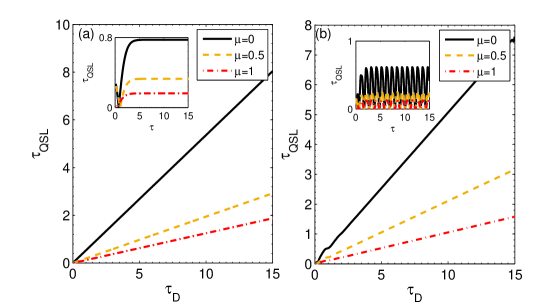
Figure 2: QSL time for correlated amplitude damping channel as a function of the driving time $\tau_{D}$ when the initial state parameters are $r=1/2$ and $\alpha=1/\sqrt{2}$ and $\tau=1$. (a)The dynamics is Markovian $\lambda/\gamma_{0}=2$(b)The dynamics is non-Markovian $\lambda/\gamma_{0}=0.2$. The inset represents the QSL time as a function of initial time $\tau$ when $\tau_{D}=1$.

In Fig. 2, the QSL time is plotted as a function of driving time $\tau_{D}$ for correlated amplitude damping channel with different values of correlation parameter $\mu$ when $\tau=1$. The inset shows the quantum speed limit time in terms of the initial time $\tau$ for different values of correlation parameter $\mu$ when $\tau_{D}=1$. In Fig. 2(a) we choose $\lambda/\gamma_{0}=2$ and the evolution is Markovian. As can be seen from Fig. 2(a), the QSL time is decreased by increasing the correlation parameter $\mu$. In Fig. 2(b) we have $\lambda/\gamma_{0}=0.2$ and the evolution is non-Markovian. As can be seen from Fig. 2(b), the QSL time is also decreased by increasing correlation parameter. From Figs. 1(a) and 2(b) one can find that for both Markovian and non-Markovian evolution the QSL time for correlated channel ($\mu=1$) is smaller than uncorrelated channel ($\mu=0$). In other word, in the presence of correlation between two successive uses of the colored pure dephasing channel on two-qubits system the quantum evolution will be faster than the case in which the correlation does not exist.
Correlated Squeezed Generalized Amplitude Damping Channels:
An amplitude damping channel represents a physical process such as energy dissipation of a two-level quantum system due to spontaneous emission of a photon into the vacuum at zero temperature Nielsen . The generalized amplitude damping (GAD) channel describes the relaxation of a quantum system when the surrounding environment is at finite temperature initially i.e., when the environment starts from a mixed state Fujiwara . Generalized amplitude damping channel is developed as a squeezed generalized amplitude damping (SGAD) channel by considering a squeezed thermal environment Srikanth . The SGAD channel is a combination of both effects of dissipation at finite temperature and environment squeezing Daffer1 ; Banerjee ; Wilson ; Banerjee1 .

The SGAD channel defines the quantum noise in which the quantum system interacts with an environment that is initially in a squeezed thermal state under the Markov and Born approximations. The dynamics of such a quantum system can be described by following Lindblad master equation

$$L(\rho_{t}) = -\frac{\Omega(n+1)}{2}(\sigma_{+}\sigma_{-}\rho_{t}+\rho_{t}\sigma_{+}\sigma_{-}-2\sigma_{-}\rho_{t}\sigma_{+})$$ (30)

$$- \frac{\Omega n}{2}(\sigma_{-}\sigma_{+}\rho_{t}+\rho_{t}\sigma_{-}\sigma_{+}-2\sigma_{+}\rho_{t}\sigma_{-})$$

$$- \Omega m(\sigma_{+}\rho_{t}\sigma_{+}+\sigma_{-}\rho_{t}\sigma_{-}),$$

where $\sigma_{+}=\frac{1}{2}(\sigma_{1}+i\sigma_{2})$ and $\sigma_{-}=\frac{1}{2}(\sigma_{1}-i\sigma_{2})$ are creation and annihilation operators, respectively, $n$ is associated with the number of thermal photons, $m$ is the squeezing parameter ($m$ and $n$ satisfy $m<n+1/2$) and $\Omega$ is the dissipation rate related to spontaneous emission at zero-temperature Breuer ; Nielsen ; Daffer1 . If $m=0$ then SGAD transforms to the GAD channel. When $m=n=0$ the SGAD channel reduces to the amplitude damping channel.

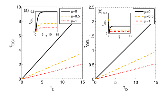
Figure 3: QSL time as a function of the driving time $\tau_{D}$ when the initial state parameters are $r=1/2$ and $\alpha=1/\sqrt{2}$ when $\tau=1$ for (a) Generalized amplitude damping channel with $m=0,n=1$ and (b) squeezed Generalized amplitude damping channel with $m=1,n=1$. The inset represents the QSL time as a function of initial time $\tau$ when $\tau_{D}=1$.

We first review the simple method for solving the master equation in Eq. (30) to find the structure of uncorrelated SGAD channel. The dynamics of single-qubit state with initial input $\rho_{0}=\sum_{i,j=0}^{1}|i\rangle\langle j|$, associated with this Lindblad master equation has the following form Daffer1

$$\rho_{t} = e^{Lt}\rho$$ (31)

$$= \sum_{i}tr(\mathcal{R}_{i}\rho)e^{\eta_{i}t}\mathcal{L}_{i}=\sum_{i}tr(\mathcal{L}_{i}\rho)e^{\eta_{i}t}\mathcal{R}_{i},$$

where $\mathcal{R}_{i}$ and $\mathcal{L}_{i}$ are the right and left eigenoperators of super-operator $L$ in Lindblad master equation, $\eta_{i}$’s are corresponding eigenvalues of these eigenoperators, such that

$$L\mathcal{R}_{i}=\eta_{i}\mathcal{R},\quad\mathcal{L}_{i}L=\eta_{i}\mathcal{L}_{i},$$ (32)

with $tr(\mathcal{L}_{i}\mathcal{R}_{j})=\delta_{ij}$. For SGAD channel, $\mathcal{R}_{i}$’s and $\mathcal{L}_{i}$’s can be defined as Jeong

$$\mathcal{R}_{1} = \frac{1}{\sqrt{2}}(\mathbf{I}_{2\times 2}-\frac{1}{2n+1}\sigma_{3}),\quad\mathcal{L}_{1}=\frac{1}{\sqrt{2}}\mathbf{I}_{2\times 2},$$

$$\mathcal{R}_{2} = \mathcal{L}_{2}=\frac{1}{\sqrt{2}}(\sigma_{+}+\sigma_{-}),$$

$$\mathcal{R}_{3} = -\mathcal{L}_{3}=\frac{1}{\sqrt{2}}(\sigma_{-}-\sigma_{+}),$$

$$\mathcal{R}_{4} = \frac{1}{\sqrt{2}}\sigma_{3},\quad\mathcal{L}_{4}=\frac{1}{\sqrt{2}}(\frac{1}{2n+1}\mathbf{I}_{2\times 2}+\sigma_{3}).$$ (33)

The eigenvalues $\eta_{i}$ are given by

$$\eta_{1} = 0,\quad\eta_{2}=-\Omega(n+m+\frac{1}{2}),$$

$$\eta_{3} = -\Omega(n-m+\frac{1}{2}),\quad\eta_{4}=-2\Omega(n+\frac{1}{2}).$$ (34)

From Eqs. (31), (32), (3.2) and (3.2), the evolved single-qubit density matrix can be quantified as

$$\rho_{t}=\left({\begin{array}[]{cc}\frac{n+p_{t}^{2}(n+1)\rho_{11}-n\rho_{22}}{2n+1}&p_{t}(q_{t}\rho_{12}-r_{t}\rho_{21})\\ p_{t}(q_{t}\rho_{21}-r_{t}\rho_{12})&1-\frac{n+p_{t}^{2}(n+1)\rho_{11}-n\rho_{22}}{2n+1}\\ \end{array}}\right),$$ (35)

where $p_{t}=e^{-\Omega(n+1/2)t}$, $q_{t}=\cosh(\Omega mt)$ and $r_{t}=\sinh(\Omega mt)$. From Eq. (35), the Kraus operators $A_{i}$ for single-qubit dynamics under SGAD channel can be written as

$$A_{1} = \left({\begin{array}[]{cc}\sqrt{\frac{n}{2n+1}+\frac{n+1}{2n+1}p_{t}^{2}-p_{t}q_{t}}&0\\ 0&0\\ \end{array}}\right),$$ (38)

$$A_{2} = \left({\begin{array}[]{cc}0&0\\ \sqrt{\frac{n+1}{2n+1}(1-p_{t}^{2})-p_{t}r_{t}}&0\\ \end{array}}\right),$$ (41)

$$A_{3} = \left({\begin{array}[]{cc}0&0\\ 0&\sqrt{\frac{n+1}{2n+1}+\frac{n}{2n+1}p_{t}^{2}-p_{t}r_{t}}\\ \end{array}}\right),$$ (44)

$$A_{4} = \left({\begin{array}[]{cc}\sqrt{p_{t}q_{t}}&0\\ 0&\sqrt{p_{t}q_{t}}\\ \end{array}}\right),$$ (47)

$$A_{5} = \left({\begin{array}[]{cc}0&\sqrt{p_{t}r_{t}}\\ \sqrt{p_{t}r_{t}}&0\\ \end{array}}\right),$$ (50)

$$A_{6} = \left({\begin{array}[]{cc}0&\sqrt{\frac{n}{2n+1}(1-p_{t}^{2})-p_{t}r_{t}}\\ 0&0\\ \end{array}}\right).$$ (53)

Now, we consider two consecutive uses of the SGAD channel on two-qubit quantum system. Uncorrelated SGAD channel $\varepsilon_{un}$ can be shown by the following Kraus operators Jeong

$$E_{ij}=A_{i}\otimes A_{j},\quad i,j=1,...,6,$$ (54)

We consider the following correlated Lindblad master equation for two-qubit system to find the structure of the correlated SGAD channel

$$\tilde{L}(\rho_{t}) = -\frac{\Omega(n+1)}{2}(\sigma_{+}^{\otimes 2}\sigma_{-}^{\otimes 2}\rho_{t}+\rho_{t}\sigma_{+}^{\otimes 2}\sigma_{-}^{\otimes 2}-2\sigma_{-}^{\otimes 2}\rho_{t}\sigma_{+}^{\otimes 2})$$ (55)

$$- \frac{\Omega n}{2}(\sigma_{-}^{\otimes 2}\sigma_{+}^{\otimes 2}\rho_{t}+\rho_{t}\sigma_{-}^{\otimes 2}\sigma_{+}^{\otimes 2}-2\sigma_{+}^{\otimes 2}\rho_{t}\sigma_{-}^{\otimes 2})$$

$$- \Omega m(\sigma_{+}^{\otimes 2}\rho_{t}\sigma_{+}^{\otimes 2}+\sigma_{-}^{\otimes 2}\rho_{t}\sigma_{-}^{\otimes 2}),$$

where $\sigma_{\pm}^{\otimes 2}=\sigma_{\pm}\otimes\sigma_{\pm}$. The correlated dynamics of a two-qubit state can be found to be similar to the single-qubit case by using Eqs.(31) and (32). We consider a general two-qubit state $\rho_{0}=\sum_{\alpha_{1},\alpha_{2}=1}^{4}\rho_{\alpha_{1},\alpha_{2}}|\alpha_{1}\rangle\langle\alpha_{2}|$ as an initial input state, where $|\alpha_{1,2}\rangle\in\left\{|00\rangle,|01\rangle,|10\rangle,|11\rangle\right\}$. The solution of correlated master equation in Eq.55 is derived as

$$\rho_{11}(t) = \frac{1}{2n+1}\left(\left((n+1)p_{t}^{2}-(2n+1)s_{t}\left(1-u_{t}\right)+n\right)\rho_{11}\right.$$

$$+ \left.\left(n-p_{t}\left(np_{t}+2(2n+1)r_{t}\right)\right)\rho_{44}\right),$$

$$\rho_{12}(t) = \sqrt{s_{t}u_{t}}\rho_{12},$$

$$\rho_{13}(t) = \sqrt{s_{t}u_{t}}\rho_{13},$$

$$\rho_{14}(t) = (\sqrt{s_{t}}u_{t}-p_{t}\left(1-q_{t}\right))\rho_{14}-p_{t}r_{t}\rho_{41},$$

$$\rho_{22}(t) = \rho_{22},$$

$$\rho_{23}(t) = \rho_{23},$$

$$\rho_{24}(t) = \sqrt{u_{t}}\rho_{24},$$

$$\rho_{33}(t) = \rho_{33},$$

$$\rho_{34}(t) = \sqrt{u_{t}}\rho_{34},$$

$$\rho_{44}(t) = 1-\rho_{11}(t)-\rho_{22}-\rho_{33}.$$ (56)

From Eq. (3.2), the Kraus operators $E_{kk}$ for correlated part is obtained as

$$E_{11} = \left({\begin{array}[]{cccc}\sqrt{s_{t}}&0&0&0\\ 0&1&0&0\\ 0&0&1&0\\ 0&0&0&\sqrt{u_{t}}\\ \end{array}}\right),$$ (61)

$$E_{22} = \left({\begin{array}[]{cccc}0&0&0&0\\ 0&0&0&0\\ 0&0&0&0\\ \sqrt{\frac{n+1}{2n+1}(1-p_{t}^{2})-p_{t}r_{t}}&0&0&0\\ \end{array}}\right),$$ (66)

$$E_{33} = \left({\begin{array}[]{cccc}0&0&0&\sqrt{\frac{n}{2n+1}(1-p_{t}^{2})-p_{t}r_{t}}\\ 0&0&0&0\\ 0&0&0&0\\ 0&0&0&0\\ \end{array}}\right),$$ (71)

$$E_{44} = \left({\begin{array}[]{cccc}\sqrt{\frac{n}{2n+1}+\frac{n+1}{2n+1}p_{t}^{2}-p_{t}(q_{t}-1)-s_{t}}&0&0&0\\ 0&0&0&0\\ 0&0&0&0\\ 0&0&0&0\\ \end{array}}\right),$$ (76)

$$E_{55} = \left({\begin{array}[]{cccc}0&0&0&0\\ 0&0&0&0\\ 0&0&0&0\\ 0&0&0&\sqrt{\frac{n+1}{2n+1}+\frac{n}{2n+1}p_{t}^{2}-p_{t}(q_{t}-1)-u_{t}}\\ \end{array}}\right),$$ (81)

$$E_{66} = \left({\begin{array}[]{cccc}\sqrt{p_{t}(q_{t})-1}&0&0&0\\ 0&0&0&0\\ 0&0&0&0\\ 0&0&0&\sqrt{p_{t}(q_{t})-1}\\ \end{array}}\right),$$ (86)

$$E_{77} = \left({\begin{array}[]{cccc}0&0&0&i\sqrt{p_{t}r_{t}}\\ 0&0&0&0\\ 0&0&0&0\\ i\sqrt{p_{t}r_{t}}&0&0&0\\ \end{array}}\right),$$ (91)

where $u_{t}=e^{-\Omega nt}$ and $s_{t}=e^{-\Omega(n+1)t}$. From Eq. (8), one can find the QSL time for correlated SGAD quantum channel after some straightforward calculation with large output . In Fig. 3, the QSL time is plotted as a function of driving time $\tau_{D}$ for correlated GAD channel and correlated SGAD channel with different values of correlation parameter $\mu$ when $\tau=1$. The inset shows the quantum speed limit time in terms of the initial time $\tau$ for different values of correlation parameter $\mu$ when $\tau_{D}=1$. In Fig. 3(a) QSL time is plotted as a function of driving time for correlated generalized amplitude damping i.e. the correlated channel with parameters $m=0,n=1$. As can be seen from Fig. 3(a), the QSL time is decreased by increasing the correlation parameter $\mu$. In Fig. 3(b) QSL time is plotted as a function of driving time $\tau_{D}$ for correlated squeezed generalized amplitude damping i.e. the correlated channel with parameters $m=1,n=1$. As can be seen from Fig. 3(b), the QSL time is also decreased by increasing correlation parameter. From Figs. 3(a) and 3(b) one can find that for both GAD and SGAD correlated channels the QSL time is decreased by increasing correlation parameter $\mu$. In other word, in the presence of correlation between two successive uses of these channels on two-qubits system the quantum evolution will be faster than the case in which the correlation does not exist.

4 Summary and conclusion

We have studied the QSL time for correlated quantum channels, where the term correlated indicates the existence of correlations between two consecutive uses of the quantum channel on a two-qubit quantum system. We have used correlated pure dephasing colored noise as an example for the unital correlated quantum channels and correlated amplitude damping and SGAD channels as the examples for the non-unital quantum channels. We found that in the case of correlated dephasing colored noise for both Markovian and non-Markovian evolution the QSL time is increased by increasing correlation parameter of quantum channel $\mu$. In other word, in the presence of correlation between two successive uses of the colored pure dephasing channel on two-qubits quantum system the quantum evolution will be slower than the case in which the correlation does not exist. In the case of correlated amplitude damping channel for both Markovian and non-Markovian evolution the QSL time is decreased by increasing correlation parameter of quantum channel $\mu$. In the case of correlated generalized amplitude damping and correlated squeezed generalized amplitude damping channel the quantum speed limit time is decreased by increasing correlation parameter of quantum channel.

References

- (1) H.-P. Breuer and F. Petruccione, The Theory of Open Quantum Systems, (Oxford Univ. Press, 2007).
- (2) U. Weiss, Quantum Dissipative Systems (3rd Edition), (World Scientific, Singapore, 2008).
- (3) V. Gorini, A. Frigerio, M. Verri, A. Kossakowski, and E. Sudarshan, Rep. Math. Phys. 13, 149 (1978).
- (4) G. Lindblad, Commun. Math. Phys. 48, 119 (1976).
- (5) G. He, J. Zhang, J. Zhu, and G. Zeng, Phys. Rev. A 84, 034305 (2011).
- (6) H. J. Carmichael, Springer-Verlag Berlin Heidelberg (Springer Berlin Heidelberg, Berlin, Heidelberg, 1999).
- (7) M. M. Wolf, J. Eisert, T. S. Cubitt, and J. I. Cirac, Phys. Rev. Lett. 101, 150402 (2008).
- (8) A. Rivas, S. F. Huelga, and M. B. Plenio, Phys. Rev. Lett. 105, 050403 (2010).
- (9) A. Rivas, S. F. Huelga, and M. B. Plenio, Rep. Prog. Phys. 77, 094001 (2014).
- (10) S. Haseli, G. Karpat, S. Salimi, A. S. Khorashad, F. F. Fanchini, B. Cakmak, G. H Aguilar, S. P. Walborn and P. H. Souto Ribeiro, Phys. Rev. A 90 (5), 052118 (2014).
- (11) S. Haseli, S. Salimi and A. S. Khorashad, Quantum Inf. Process. 14: 3581 (2015).
- (12) S. Haseli, S. Salimi, A. S. Khorashad and F. Adabi, Int. J. Theor. Phys. 55: 4089 (2016) .
- (13) F. F. Fanchini, G. Karpat, B. Çakmak, L. K. Castelano, G. H. Aguilar, O. J. Farías, S. P.Walborn, P. H. S. Ribeiro, and M. C. de Oliveira, Phys. Rev. Lett. 112, 210402 (2014).
- (14) N. Lambert, Y.-N. Chen, Y.-C. Cheng, C.-M. Li, G.-Y. Chen, and F. Nori, Nat. Phys. 9, 10 (2013).
- (15) M. Thorwart, J. Eckel, J. Reina, P. Nalbach, and S. Weiss, Chem. Phys. Lett. 478, 234 (2009).
- (16) S. F. Huelga and M. B. Plenio, Contemp. Phys. 54, 181 (2013).
- (17) R. Vasile, S. Olivares, M. A. Paris, and S. Maniscalco, Phys. Rev. A 83, 042321 (2011).
- (18) A. W. Chin, S. F. Huelga, and M. B. Plenio, Phys. Rev. Lett. 109, 233601 (2012).
- (19) B. Hwang and H.-S. Goan, Phys. Rev. A 85, 032321 (2012).
- (20) C. Macchiavello and G. M. Palma, Phys. Rev. A 65, 050301(R) (2002).
- (21) F. Caruso, V. Giovannetti, C. Lupo, and S. Mancini, Rev. Mod. Phys. 86, 1203, (2014).
- (22) D. Kretschmann and R. F. Werner, Phys. Rev. A 72, 062323 (2005).
- (23) C. Addis, G.Karpat, C. Macchiavello, and S. Maniscalco, Phys. Rev. A 94, 032121 (2016).
- (24) M. Ramzan, Quantum Inf. Process. 12, 83-95 (2013).
- (25) Y.-n. Guo, M.-f. Fang, G.-y. Wang and K. Z. Quantum Inf. Process. 15: 5129 (2016).
- (26) G. Karpat, Canadian Journal of Phys. 96(7): 700-704 (2018).
- (27) Y. Guo, M. Fang, K. Zeng, arXiv:1710.06344.
- (28) L. Mandelstam and I. G. Tamm, J. Phys. (USSR) 9, 249 (1945).
- (29) N. Margolus and L. B. Levitin, Physica (Amsterdam) 120D, 188 (1998).
- (30) V. Giovannetti, S. Lloyd and L. Maccone, Phys. Rev. A 67, 052109 (2003).
- (31) M.M. Taddei, B.M. Escher, L. Davidovich, and R. L. de Matos Filho, Phys. Rev. Lett. 110, 050402 (2013).
- (32) B. M. Escher, R. L. de Matos Filho, and L. Davidovich, Nat. Phys. 7, 406 (2011).
- (33) S. Deffner and E. Lutz, Phys. Rev. Lett. 111, 010402 (2013).
- (34) A. del Campo, I. L. Egusquiza, M. B. Plenio, and S. F. Huelga, Phys. Rev. Lett. 110, 050403 (2013).
- (35) Y. Zhang, W. Han, Y. Xia, J. Cao, H. Fan, Sci. Rep. 4, 4890 (2014).
- (36) Z. Y. Xu, S. Q. Zhu, Chin. Phys. Lett. 31, 020301 (2014).
- (37) D. Mondal and A. K. Pati, arXiv: 1403.5182.
- (38) L. B. Levitin and T. Toffoli, Phys. Rev. Lett. 103, 160502 (2009).
- (39) Z. Y. Xu, S. Luo, W. L. Yang, C. Liu and S. Zhu, Phys, Rev. A 89, 012307 (2014).
- (40) X. Meng, C. Wu, and H. Guo, arXiv:1404.4241.
- (41) N. Mirkin, F. Toscano, D. A. Wisniacki, Phys. Rev. A 94, 052125 (2016).
- (42) F. Campaioli, F. A. Pollock, K. Modi, Quantum 3, 168 (2019).
- (43) R. Uzdin, R. Kosloff, EPL, 115, 40003 (2016).
- (44) K. M. R. Audenaert, Quant. Inf. Comp. 14, 31-38 (2014).
- (45) C. Liu, Z.-Y. Xu, S. Zhu, Phys. Rev. A 91, 022102 (2015).
- (46) J. Anandan and Y. Aharonov, Phys. Rev. Lett. 65, 1697 (1990).
- (47) J. M. Steele, The Cauchy–Schwarz Master Class: an Introduction to the Art of Mathematical Inequalities". The Mathematical Association of America. p. 1. ISBN 978-0521546775, (2004).
- (48) R. Bhatia, Matrix Analysis, (Springer, Berlin, 1997).
- (49) B. Simon, Trace Ideals and their Applications, (Springer, Berlin, 2005).
- (50) Y. Yeo, A. Skeen, Phys. Rev. A 67, 064301 (2003).
- (51) N. Awasthi, U. C. Johri, arXiv:1807.07782.
- (52) M. A. Nielsen, I. L. Chuang, Quantum Computation and Quantum Information, 10th anniversary edn. (Cambridge University Press, New York, 2010).
- (53) S. Imre, L. Gyongyosi, Advanced Quantum Communications (An Engineering Approach). Wiley, New York, NY (2012).
- (54) C. King, M.B. Ruskai, IEEE Trans. Inf. Theory 47, 192–209 (2001).
- (55) S. Daffer, K. Wodkiewicz, J. D. Cresser, J. K. Mclver, Phys. Rev. A 70, 010304(R) (2004).
- (56) A. Fujiwara, Phys. Rev. A 70, 012317 (2004).
- (57) R. Srikanth, S. Banerjee, Phys. Rev. A 77, 012318 (2008).
- (58) S. Daffer, K. Wodkiewicz and J. K. McIver, Phys. Rev. A 67, 062312 (2003).
- (59) S. Banerjee and R. Ghosh, J. Phys. A: Math. Theor. 40, 13735–13754 (2007).
- (60) D. Wilson, J. Lee and M. S. Kim, J. Mod. Opt. 50, 1809–1815 (2003).
- (61) S. Banerjee, V. Ravishankar and R. Srikanth, Ann. Phys. 325, 816–834 (2010).
- (62) Y. Jeong and H. Shin, Sci. Rep. 9, 4035 (2019).